Growth of a massive young stellar object fed by a gas flow from a companion gas clump

Abstract

We present a Submillimeter Array (SMA) observation towards the young massive double-core system G350.69-0.49. This system consists of a northeast (NE) diffuse gas Bubble and a southwest (SW) massive young stellar object (MYSO), both clearly seen in the Spitzer images. The SMA observations reveal a gas flow between the NE Bubble and the SW MYSO in a broad velocity range from 5 to 30 km s^-1with respect to the system velocity. The gas flow is well confined within the interval between the two objects, and traces a significant mass transfer from the NE gas Bubble to the SW massive core. The transfer flow can supply the material accreted onto the SW MYSO at a rate of $4.2\times 10^{-4}~{}M_{\odot}$ year^-1. The whole system therefore suggests a mode for the mass growth in MYSO from a gas transfer flow launched from its companion gas clump, despite that the driving mechanism of the transfer flow is not yet fully determined from the current data.

1. Introduction

Massive stars (O and B stars) contribute to the important feedback initially on the star cluster, and ultimately drive the overall evolution of the host galaxy through their strong outflows, stellar winds and ionizing radiations (Kennicutt 2005). Due to short Kelvin-Helmholtz time scale, the massive young stellar objects (MYSOs) will experience a drastic bloating phase, during which the stellar radius expands for $\sim 30$ times larger and then rapidly contract back to form the zero-age main sequence star (Behrend & Maeder 2001; Hosokawa & Omukai 2009; Kuiper & Yorke 2013). During the entire process of massive star formation, how to maintain the stable accretion to form the observed high-mass stars is thus a major question to be concerned.

The mechanism for mass growth of massive forming star is still in debate (see review papers, e.g., Zinnecker & Yorke 2007; Tan et al. 2014). Different scenarios have been proposed to explain their high masses, such as stellar collisions and mergers in very dense systems (Bonnell et al. 1998), monolithic collapse like in low-mass star formation (Yorke & Sonnhalter 2002; McKee & Tan 2003), and competitive accretion in a proto-cluster environment (Bonnell et al. 2001, 2004; Bonnell & Bate 2006). Accretion disks are expected at small scales in the both scenarios, i.e., the monolithic core collapse and competitive accretion. Recently the field of theoretical understanding of accretion in massive star formation has made clear process. However, two competing theories for accretion are currently in conflict with each other: the formation of the most massive stars via radiative Rayleigh-Taylor unstable outflows (Krumholz et al. 2009, Rosen et al. 2016) and via disk-mediated accretion (Nakano 1989, Yorke & Bodenheimer 1999, Yorke & Sonnhalter 2002, Kuiper et al. 2010, 2011). Both scenarios solve the radiation-pressure problem of spherically symmetric accretion flows via an anisotropy in the thermal radiation field. The latter disk accretion scenario has been observationally supported by e.g. Johnston et al. (2015), while the radiative Rayleigh-Taylor instability scenario is supported by Kumar (2013).

On larger scales, the star-forming core should have a sufficient mass storage to feed the central star and should not be dissipated by the stellar emission and outflow. One possibility is that the cores obtain mass from its surrounding cores and/or the natal gas clump. A representative model for this process is competitive accretion (e.g., Bonnell & Bate 2006). However, till now the external gas supply is not fully confirmed in observations. This should be mainly because the external gas flow into the core cannot be so easily identified. In several ideal cases, prominent converging flows into the hub or dense center of the filamentary structures have been observed (e.g. Kirk et al. 2013; Peretto et al. 2013), which strongly suggests gas inflow from the surrounding extended gas structures that is feeding the central young stars. Yet it still calls for more extensive studies to reveal two major properties, including 1) the specific gas motions in the intermediate neighborhood of individual cores, whether and how the accretion flow enters the cores; 2) the dynamical cause of the inflow, whether it was driven by cloud collision, magnetic field or purely due to the gravitational collapse.

In this paper, we present the observational results towards a massive double-core system (G350.69-0.49, G350.69 hereafter), which for the first time, exhibits an evident mass transfer flow launched from the one core to supply the mass growth of its companion core which is a MYSO. The double-core system shows extended shock-excited 4.5 $\mu$m emission (Extended Green Object; EGO) identified from the Spitzer GLIMPSE II survey (Chen et al. 2013). In Section 2 we described the observation and data reduction for the observational data. In Section 3 we presented the overall structure of dust and gas distribution for this source. The kinematic features and their possible origins are more specifically discussed in Sections 4 and 5. A summary is given in Section 6.

2. Observation and Data Reduction

The SMA observations of G350.69 were carried out on 2014 May 5th in its compact array configuration. The calibration of the time dependent antenna gains was performed by frequent observations of quasars 1700-261 and 1744-312. The bandpass response was calibrated using the standard calibrator quasar 3C279; and the absolute flux density was scaled by comparing with the modelled ones of Neptune and Titan. The two 4-GHz sidebands were centered at 219 and 229 GHz, respectively. The channel width is 0.812 MHz, corresponding to a velocity resolution of 1.1 km s^-1 at 230 GHz. The on-source integration time was 4.3 hours. The visibility data were calibrated using the IDL superset MIR. The imaging and analysis were carried out in MIRIAD. The synthesized beam size, i.e., the angular resolution of the image data is $5.1^{\prime\prime}\times 2.9^{\prime\prime}$ with a position angle of $7^{\circ}$ northwest and the rms noise is 50 mJy beam^-1 per-channel for the molecular line data, and 3 mJy beam^-1 for the 1.3 mm continuum.

The continuum emissions of G350.69 from mid- to far-infrared were also acquired, including the Spitzer/IRAC images and the Herschel PACS 70, and 100 $\rm\mu m$, SPIRE 250, 350, and 500 $\rm\mu m$ images .

3. Overall morphology

3.1. Spitzer and Herschel images

The Spitzer image of three-color composite at three IRAC bands for the source G350.69 is presented in Figure 1a. It can be clearly seen that this source resembles a binary system, containing a northeast (NE) diffuse object and a southwest (SW) compact object. There is a rather strong extended 4.5 $\micron$ emission (green feature in the three-band RGB image) in the gap between the two middle-infrared (MIR) objects along the northeast-southwest (NE-SW) direction. There are other two 4.5 $\micron$ emission features along northwest-southeast (NW-SE) direction approximately perpendicular to the above mentioned NE-SW direction. As suggested by previous works (Cyganowski et al. 2008; Chambers et al. 2009; Chen et al. 2013), the excessive 4.5 $\micron$ features should reveral the shock emission as induced by the supersonic material flow along these directions.

The SW compact object should contain an MYSO due to its association with a 6.7 GHz class II methanol maser (Minier et al. 2003; Xu et al. 2007), which is known to be an exclusive MYSO tracer. This object also coincides with a point source seen in Spitzer 24 and 8 $\micron$, suggesting an embedded protostar in a dust envelope (Chambers et al. 2009). The NE diffuse component shown in IRAC 8 $\micron$ emission (Figure 1a) is identified as an MIR Bubble (Churchwell et al. 2006, 2007). Dynamically formed Bubbles with bright MIR emission require a star or cluster with UV emission to excite the polycyclic aromatic hydrocarbon (PAH) features in the 5.8 and 8.0 $\micron$ bands (Churchwell et al. 2006). Based on its small angular diameter of $\sim 30^{\prime\prime}$ (corresponding to 0.4 pc, at a near kinematic distance of 2.7 kpc to this source, see Chen et al. 2013) and non-detections of Hii region tracers, such as the centimeter emission and radio recombination lines (Condon et al. 2008; Anderson et al. 2011), this Bubble should be produced by a young hot late-B (below B4) star that failed to produce a detectable Hii region, but is still sufficiently intensive to blow a small dust Bubble via radiation pressure (Churchwell et al. 2007). Alternatively, the central star may be massive pre-main-sequence star that is in a bloating stage thus has a relatively low temperature (Kuiper & York 2013), thereby a low ionization rate. But it may have intense stellar wind and/or a high total luminosity in order to generate the dusty Bubble.

The Herschel PACS 70 $\micron$ image is presented in Figure 1b. The 70 $\micron$ emission region is reasonably coincident with the Bubble seen in 8 $\micron$ emission. A closer look shows that the emission is more intense towards its southwest side. This feature is also likely seen in the Herschel images at longer wavelengths despite their lower resolutions, such as the SPIRE 500 $\micron$ images as shown in Figure 1c. It may reflect the trend that the Bubble material is being concentrated around Core-2, the mass concentration is consistent with ¹³CO $(2-1)$ emissions (see below).

3.2. Millimeter Continuum and Gas distribution

The integrated ¹³CO emission and continuum emission observed with the SMA are also shown in Figure 1. The ¹³CO emission exhibits an arc-shaped structure surrounding the edge of the IRAC 8 $\micron$ gas Bubble. Such a phenomenon has also been seen in other MIR Bubble objects. The arc-shaped emission should represent a cold gas-and-dust Bubble believed to surround the central hot gas (Ji et al. 2012; Dewangan et al. 2012; Dewangan & Ojha 2013; Xu & Ju 2014; Yuan et al. 2014; Liu et al. 2016). The UV emission should have largely destroyed the molecules within the MIR Bubble (with a temperature of a few 1000 K), thus no emission of molecular gas can be seen from it.

Two significant dust continuum cores are detected in this binary system: one is coincident with the SW MYSO (denoted as Core-1), another near the edge of the MIR Bubble (denoted as Core-2). Core-1 is a single, compact object. Using a two-dimensional Gaussian profile to fit its 1.3 mm emission region (Using the imfit task in miriad), we obtained a spatial size of $(b_{\rm maj},b_{\rm min})=(3.3^{\prime\prime},2.4^{\prime\prime})$. The size of Core-2 is fitted to be $(5.2^{\prime\prime},4.0^{\prime\prime})$, suggesting that it is more extended than Core-1. The extent of the Bubble is measured from its IRAC 8 $\micron$ emission (Figure 1a). The results are shown in Table 1.

3.3. Core masses

The Spectral Energy Distributions (SEDs) of the cores can be constructed from their flux densities in the Herschel bands. Based on the radiative transfer equation, the flux density of the dust core from a gray-body emission model (Hildebrand 1983) is

$$S_{\nu} =\kappa_{\nu}B_{\nu}(T_{\rm d})\Omega\mu m_{\rm H}N_{\rm tot}$$ (1)

$$=\frac{\kappa_{\nu}B_{\nu}(T_{\rm d})M_{\Omega}}{D^{2}},$$

wherein $S_{\nu}$ is the flux density at the frequency $\nu$. $\Omega$ is the solid angle of the core or selected area. $B_{\nu}(T_{\rm d})$ is the Planck function of the dust temperature $T_{\rm d}$, $N_{\rm tot}$ is the gas column density (mostly HI+${\rm H_{2}}$), $\mu=2.33$ is the mean molecular weight (Myers 1983). $m_{\rm H}$ is the mass of the hydrogen atom. $\kappa_{\nu}$ is the dust opacity; it is assumed to be related with the frequency in the form $\kappa_{\nu}=\kappa_{\rm 230GHz}(\nu/{\rm 230GHz})^{\beta}$. The reference value $\kappa_{\rm 230GHz}=0.009$ cm² g^-1, is adopted from dust model for the grains with coagulation for $10^{5}$ years with accreted ice mantles at a density of $10^{6}$ ${\rm cm^{-3}}$ (Ossenkopf & Henning 1994). $D=2.7$ kpc is the source distance (Chen et al. 2013). We note that the near distance from the Galactic rotation curve is adopted. Another $D=10.9$ kpc, would cause the core masses to be unreasonably high. For example, at $D=10.9$ kpc, Core-2 mass would be $M\simeq 1400~{}M_{\odot}$, which largely exceeds the most massive cores (e.g. $M\simeq 500~{}M_{\odot}$ in Perreto et al. 2013).

The apertures to measure the flux densities are plotted in dashed lines in Figure 2b. The Bubble is overlapped with Core-2. Assuming a uniform brightness over the Bubble surface, $S_{\rm Core2}$ was measured by subtracting the background emission measured from the bubble surface away from Core-2. And for the Bubble, we have $S_{\rm Bubble}=S_{\rm Bubble+Core2}-S_{\rm Core2}$, wherein $S_{\rm Bubble+Core2}$ is their total flux density measured within the largest circle shown in Figure 2b.

The SED fitting is mainly affected by the flux uncertainties, which should be evaluated. The uncertainties mainly include three factors, including the rms noise over the image ($\Delta S_{\rm rms}$), the errors in flux calibration ($\Delta S_{\rm cal}$), and the low angular resolution that blends different cores ($\Delta S_{\rm res}$). And the total uncertainty is $\Delta S_{\rm tot}^{2}=\Delta S_{\rm rms}^{2}+\Delta S_{\rm cal}^{2}+\Delta S_{\rm res}^{2}$. In G350.69, the uncertainties were found to be dominated by the third part since the cores are poorly resolved in the Herschel bands. In order to estimate its scale, we assumed each object to originally have a 2D Gaussian distribution with the half-maximum diameter same as that shown in Table 1.

The model image is convolved with the beam size and regridded with the pixel size in each band. And then we compared the flux measurement between the modeled and the observed images, and the difference between the two may roughly represent the uncertainty. We note that the modeled image cannot represent the real dust distribution but is only used to estimate the flux uncertainties. As a result, the uncertainty scales ($\Delta S_{\rm res}/S_{\nu}$) are from 10% to 150% for 70 to 500 $\micron$ bands. The flux calibration uncertainties ($\Delta S_{\rm cal}/S_{\nu}$) are around 5% to 10% for the Herschel bands (see PACS and SPIRE manuals, also described in Ren & Li 2016, Appendix A.1 therein). The rms level is measured to be $5-20$ mJy beam^-1 throughout the Herschel bands. Its contribution to $\Delta S_{\rm tot}$ is much less significant than the other two terms. The measured flux densities are shown in Table 2.

Although the flux measurement in the SPIRE bands has large uncertainties due to the poor resolutions (Figure 2c), it does not largely increase the $T_{\rm d}$ uncertainty mainly because the SED is more closely constrained by the emissions in shorter wavelengths (PACS bands). For each body, the observed flux densities can be well reproduced using a single $T_{\rm d}$ component. $\beta$ and $M_{\rm 70\micron}$ are also inferred from the SED fitting. The results are presented in Table 1.

The masses of Core-1 and Core-2 are calculated also using the 1.3 mm emissions, which should represent the masses of the compact gas components. The Bubble is not detected in 1.3 mm due to insufficient uv coverage for short baselines.

The column density $N({\rm H_{2}})$ of the three objects at their centers are all calculated from the 70 $\micron$ using Equation (1). The values of Core-1 and Core-2 are also derived from the 1.3 mm intensities. And the number densities $n({\rm H_{2}})$ are then derived using $n({\rm H_{2}})=N({\rm H_{2}})/\bar{d}$, where $\bar{d}$ is the average diameter of the core that is $\bar{d}=(b_{\rm maj}+b_{\rm min})/2$. The value should represent the average number density at the center along the line of sight.

4. Kinematical properties

4.1. Mass transfer flow

Figure 3a and 3b show the velocity-integrated ¹²CO emissions in different velocity ranges. The velocity ranges of these components can be determined from the Position-Velocity diagrams as shown in Figure 3c.

The PV1 direction (Figure 3c, upper panel) shows that the gas flow is distributed in a broad velocity range, extending from $|\Delta V|=5$ to 30 km s^-1 from the central velocity ($V_{\rm sys}=-19$ km s^-1). The low- and high-velocity components are observed to have distinct morphologies. The low-velocity components have $|\Delta V|<15$ km s^-1  and are distributed in both blue- and red-shifted sides. Whereas the high-velocity component is only observed in the blueshifted side and is less intense than the low-velocity components. It is located between Core-1 and Core-2 and with a velocity range of $\Delta V=10-30$ km s^-1.

The integrated emissions of the low-velocity components (Figure 3a) are mainly extended from Core-1 to Core-2. The components along the PV-1 direction are roughly symmetrically distributed around Core-2. The blueshifted emission extends to Core-2 and is almost rightly terminated at Core-1 center. Another blueshifted emission feature is to the east of Core-2 at offset=$(-15^{\prime\prime},0^{\prime\prime})$. This feature is also seen in ¹³CO and C¹⁸O and should trace the gas condensation in the Bubble shell. Figure 3b shows a very compact morphology of the high-velocity flow between Core-1 and Core-2. There are no other emission features in this velocity range.

In PV2 direction there are two gas lobes symmetrically distributed with respect to Core-1. They are $20^{\prime\prime}$ distant from Core-1 center (Figure 3a). The two lobes also have comparable velocity ranges ($\Delta V=2$ to 12 km s^-1) and intensities as shown in Figure 3c (lower panel). They should represent a bipolar outflow ejected from Core-1. It is noticed that each outflow lobe has both red- and blueshifted emissions. This may suggest that the outflow axis is close to the plane of the sky, so that each lobe can exhibit opposite gas motions as projected along the line of sight.

The SiO $(5-4)$ and H₂CO (3-2) emissions and PV diagrams are shown in Figure 4. The two species both have compact emission regions around Core-1 and Core-2 (Figure 4a), but largely differ in their velocity distributions (Figure 4b). The SiO emission has a large fraction extending to the blueshifted side up to $\Delta V=10$ km s^-1 (Figure 4b, upper panel). Similar with the high-velocity ¹²CO flow, the blueshifted SiO emission is also confined between Core-2 and Core-1. In comparison, the H₂CO has only one narrow velocity component emission around the $V_{\rm sys}$ from Core-2 to Core-1, despite that it also has weak emissions to the blueshifted side.

The SiO emission also suggests that the mass transfer flow is launched from Core-2 to Core-1. At the Core-2 center (offset$=12^{\prime\prime}$ in the PV diagram, Figure 4b), the SiO emission feature continuously extend from $V_{\rm lsr}=-18$ to $-25$ km s^-1. While at Core-1 (offset$=0^{\prime\prime}$) there is apparently a velocity gap between the blueshifted emission $(-27,-21)$ km s^-1 and the Core-1 emission $(-20,-15)$ km s^-1. A reasonable explanation is that the mass transfer flow is being braked at Core-1 so that the velocity distribution is also interrupted. In fact, as seen in Figure 3c, the high-velocity component in ¹²CO is also connected with Core-2, likely being accelerated and terminated towards Core-1. The fact that mass transfer flow is started from Core-2 and terminated at Core-1 suggests that it could supply the mass for the star formation in Core-1.

Assuming the mass transfer flow to have a cylindrical shape that links Core-1 and Core-2, the corresponding mass transfer rate to Core-1 can be approximately derived using $\dot{M}_{\rm trans}=\mu m_{\rm H_{2}}N_{\rm H_{2}}d_{\rm flow}\bar{v}_{\rm flow}$. Here $N_{\rm H_{2}}$ is the gas column density in the region of the transfer flow, $d_{\rm flow}$ is the average diameter of the flow cross section, $\bar{v}_{\rm flow}$ is the average flow velocity. In calculation, we adopt $N_{\rm H_{2}}=5\times 10^{22}$ cm^-2 which is derived from the 1.3 mm dust emission between Core-1 and Core-2 ($\sim$0.014 Jy beam^-1). The flow diameter $d_{\rm flow}$ is adopted as width of the SiO emission region (Figure 4a) deconvolved with the beam size, that is $d=5.0^{\prime\prime}$ ($\sim$14000 AU). The flow velocity is adopted as the mean velocity of the low-velocity component in ¹²CO ($v_{\rm flow}=7$ km s^-1 as measured from Figure 3c). Based on these values, we estimate the mass transfer rate of 4.2$\times 10^{-4}$ $M_{\odot}$ yr^-1.

We note that the ¹²CO blue lobe (Figure 3a) apparently has a larger width than the SiO emission region, namely a larger $d_{\rm flow}$. It would imply a higher mass transfer rate if the gas traced by the ¹²CO blue lobe can be all obtained by Core-1.

4.2. Core rotation and Bipolar outflow from Core-1

The integrated emission region and the intensity-weighted velocity field (moment-1 map) of the C¹⁸O (2-1) are shown in Figure 5a. The PV diagrams of the C¹⁸O and ¹³CO lines are shown in Figure 5b. The C¹⁸O shows a linear velocity gradient throughout Core-1, with the radial velocity range of $V_{\rm lsr}=(-18.5,-16)$ km s^-1 through Core-1 from its northeast to southwest. The velocity gradient should indicate the core rotation with an average velocity of $V_{\rm lsr}=1.2$ km s^-1.

Comparing with Figure 3a, one can see that the two outflow lobes of the ¹²CO in PV2 direction are actually aligned quite well along the rotational axis. This suggests that Core-1 may contain a disk-jet system, with the mid-plane roughly in parallel with the direction from Core-2 to Core-1. The velocity at northeast edge of Core-1 is smoothly connected with the mass transfer flow arrived on its edge (Figure 5b, upper panel). This suggests that the mass transfer flow may be also bringing angular momentum into Core-1, thereby help sustain or enhance its rotation.

Assuming a ¹²CO abundance of $10^{-4}$ and an excitation temperature similar with the Core-1 dust temperature (21 K, see Table 1), the masses of the two outflow lobes were estimated to be $M=0.5$ and 0.7 $M_{\odot}$, for the blue and red lobes, respectively. From their average velocity ($\sim$ 6 km s^-1) and distance ($\sim 15^{\prime\prime}$, corresponding to $4\times 10^{4}$ AU) from Core-1, the time scale of the outflow is estimated to be $t_{\rm out}=4.8\times 10^{4}$ year, and the outflow rate is $\dot{M}_{\rm out}=M_{\rm out}/t_{\rm out}\simeq 2\times 10^{-5}~{}M_{\odot}$ year^-1, which is much smaller than the mass transfer rate due to the gas flow. This suggests that Core-1 should be dominated by the transfer flow thus in a mass growth.

5. Discussion: Origination of the transfer flow

5.1. Possibility: An outflow from Core-2

The first possibility is that the transfer flow between the two cores is a part of jet-like outflow driven by an embedded protostar in Core-2 on the Bubble edge. It is in a morphological agreement with the low-velocity ¹²CO components that have symmetric blue- and red-shifted emission regions around Core-2 (see Figure 3a). However, it should be questioned why the high-velocity flow (Figure 3b) does not have a redshifted counterpart on the northeast side of Core-2. There are three possible causes for such asymmetry. First, the high-velocity outflow might be intrinsically unipolar or has a very weak red lobe. Second, the blue lobe might be dissipated in the hot Bubble. Third, the high-velocity flow could be compressed by the infalling gas into Core-2.

The second and third cases both anticipate the outflow to have a significant interaction with the Bubble or infalling gas. Then we would expect them to generate shocked region. However, the redshifted CO outflow lobe is not evidently detected in either SiO or IRAC 4.5 $\micron$ emission, suggesting that the gas interaction between Core-2 and the Bubble is not significant, or at least weaker than that between Core-1 and Core-2.

5.2. Possibility: A Roche overflow

Another possible kinematics process for the observed mass transfer flow is that the material is the Roche overflow from the MIR Bubble to the Core-1. This scenario is proposed mainly based on the two distinct features which are already shown above: (1) a gas flow from Core-2 and Core-1 with broad velocity range, (2) the rotation and bipolar outflow in Core-1. Based on these two features, the entire system vividly resembles a binary system with the Roche overflow exceeding the Lagrange L1 point to accrete onto the companion star. The likelihood of such scenario can be evaluated based on the geometry and the core masses.

A critical position in the Roche-overflow system is the Lagrange point L1, where the gravities from the two objects reach a balance. If the material from one of the binary members moves over this point, it would accrete onto the companion object if there are no other perturbations. The distance from L1 to Core-1 center $r$ can be estimated using the equation:

$$\frac{M_{2}}{(R-r)^{2}}=\frac{M_{1}}{r^{2}}+\frac{M_{2}}{R^{2}}-\frac{r(M_{1}+M_{2})}{R^{3}},$$ (2)

wherein $R$ is the distance between the two companions, $M_{1}$ and $M_{2}$ are their masses (assuming $M_{2}>M_{1}$ without losing generality). In G350.69, the masses are adopted to be $M_{2}=M_{\rm Core2+Bubble}$ and $M_{1}=M_{\rm Core1}$, using the masses measured from the 70 $\micron$ continuum (see Table 1). The mass center of $M_{2}$ is relatively uncertain, and we considered two limits that the $M_{2}$ center varies from the Bubble center to the Core-2 center.

Figure 6 shows the $M_{2}$ position and the corresponding L1 point range, which extends from the Bubble edge to the interval between Core-2 and Core-1. Since the SiO and ¹³CO emissions are all continuously distributed from Core-1 to Core-2, the gas flow would obviously propagate over L1 and accretes onto Core-1.

In the classical condition of a Roche overflow, the gas motion is determined by the equivalent gravity field in the binary system. To examine this, we made a simple model to estimate the gas velocity from the core masses and compare it with the observed velocity distribution. We first calculated the gravitational potential field due to the four gas components:

(1). The Bubble which is assumed to be concentrated within a half-elliptical shell with number density $n_{\rm 0,Bubble}$, and its projected image was adjusted to be best coherent with the ¹³CO image.

(2,3). The dense inner components of Core-1 and Core-2, which have uniform density and radii equal to the deconvolved radii of the SMA 1.3 mm cores.

(4). The envelope of Core-1, which has a power-law density profile out of $r_{\rm Core-1}$, that is $n(r)=n_{\rm 0}(r/r_{\rm 0})^{-p}~{}(r>r_{0})$, wherein the power-law index is adopted to be $p=-1.1$, as the average value for the massive molecular cores (Butler & Tan 2012). We note that the extended gas around Core-2 should be included in the Bubble shell, thus an envelope for Core-2 was no more separately modelled.

For each component, its reference number density $n_{0}$ is adjusted so that the total mass is consistent with the observed value. For the envelope of Core-1, the mass should be $M_{\rm env}=M_{70\micron}-M_{1.3mm}=13~{}M_{\odot}$ (see Table 1). The surface contour of each component is shown in Figure 7a. The projected gas distribution on the X-Y plane is shown in Figure 7b, wherein the integrated ¹³CO emission is also overlaid.

In the reference frame co-rotating with the two cores, the equivalent potential well out of the core boundaries ($|{\bf r}|>r_{\rm core1}$ and $|{\bf r-R_{12}}|>r_{\rm core2}$) is:

$$\phi_{\rm cores}({\bf r})= -\frac{GM_{1}}{|{\bf r}|}-\frac{GM_{2}}{|{\bf r-R_{12}}|}$$ (3)

$$-\frac{1}{2}[\Omega\times({\bf r}-\frac{M_{1}{\bf R_{12}}}{M_{1}+M_{2}})]^{2},$$

wherein ${\bf R_{12}}$ is the distance vector from Core-1 to Core-2, $\Omega$ is the angular velocity of their rotation. It is estimated from the velocity difference between Core-1 and Core-2 and their distances assuming an inclination angle of $45^{\circ}$ with respect to the line of sight. And the masses are $M_{1,2}=M_{\rm Core1,Core2}$ in 1.3 mm because the Equation (5) is only for the dense cores (the extended component is modeled in Equation (6) as following).

The second contribution is from more extended gas components, including the Bubble and the Core-1 envelope that is not sampled in the SMA 1.3 mm continuum. The potential field is numerically sampled using

$$\phi_{\rm ext}({\bf r})=-G\int\frac{{\rm d}M({\bf r_{\rm ext}})}{|{\bf r-r_{\rm ext}}|}.$$ (4)

The integration is numerically performed for the Bubble and the envelope in the model. And the total potential is

$$\phi({\bf r})=\phi_{\rm cores}({\bf r})+\phi_{\rm ext}({\bf r}).$$ (5)

For the fraction of gas that is falling into the cores originally from Bubble center, the gas velocity purely due to $\phi({\bf r})$ would be

$$v_{\rm inf}({\bf r})=\sqrt{2[\phi({\bf r_{0}})-\phi({\bf r})]},$$ (6)

wherein ${\bf r_{0}}$ is the vector distance form Core-1 center to the Bubble center. We note that owing to the viscosity deceleration and the projection effect, the modelled velocity field should represent the upper limit for the observed velocity along the line of sight. The derived velocity distribution is shown in Figure 7c. The highest velocity is reached at Core-2 center, and Core-1 center also has a local maximum of $v_{\rm inf}\simeq 4$ km s^-1, which are both within our expectation.

Figure 7d to 7f show the observed ¹²CO, ¹³CO and SiO velocity distribution from Core-2 to Core-1, respectively (same as the PV diagrams shown in Figure 3 to 5). The modelled velocity profile is overlaid in red-square line. One can see that for the ¹³CO (2-1) and SiO (5-4) line, the calculated velocity profile is reasonably consistent with the maximum value of the gas flow, except for that a fraction of the SiO (5-4) emission is beyond the modelled curve around Core-1. For the ¹²CO (2-1), the blueshifted emission feature, in particular the high-velocity component, largely exceeds the modelled curve. This indicates that the high-velocity component of the flow cannot be generated solely by the gravity of the two cores.

Besides an outflow from Core-2, the central star in the Bubble an also accelerate the mass transfer flow. In the case of Roche overflow, the gas could be originally pushed towards the Roche lobe boundary by the radiation pressure and/or stellar wind from the central star in the Bubble. In this case, Roche lobe boundary should be largely overlapped with the observed bubble shell (Figure 5a). The gas would be compressed onto the shell except at the L1 point, wherein the gas can directly move to Core-1 due to the Roche overflow and is not accumulated therein. Therefore, the driving force from the central star would accelerate the flow without resistance, forming the high-velocity flow as observed. In the mean time, the materials on the shell would slowly slide onto the L1 point and join into the transfer flow.

As a short summary for the mass transfer flow, the gravity from Core-1 and Core-2 would be almost sufficient to pull the gas from the Bubble and generate the low-velocity mass transfer flow. Whereas the high-velocity flow is likely to require an additional driving force. The outflow from Core-2 might be a possible case, while the stellar wind and radiation from the progenitor star of the Bubble is also a considerable factor. We note that the low-velocity flow is much more intense than the high-velocity part and would contribute a major fraction of the mass transfer rate.

5.3. Contribution to the Mass Growth in Core-1

Although we can not fully determine the initial driving mechanism for the mass transfer flow from the current data, the observations reveal that the Core-1 is obtaining mass via the transfer flow and has likely formed a disk-outflow system in its accretion. In an isolated isothermal collapsing core, the mass infall would reach a maximum if the entire core is in a free-fall collapse, that is $\dot{M}\approx M_{dc}/t_{\rm ff}$, wherein $t_{\rm ff}=[3\pi/(32G\rho)]^{1/2}$ is the free-fall time, calculated to be $t_{\rm ff}\simeq 1.2\times 10^{5}$ years. For Core-1, using the density from the 1.3 mm continuum ($\rho=3.0\times 10^{-18}$ $g$ cm^-3, see Section 3.3 and Table 1), the mass infall rate is derived to be 5.0$\times 10^{-4}$ $M_{\odot}$ yr^-1. This value is comparable with the mass transfer flow ($4.2\times 10^{-4}$ M_⊙ yr^-1), suggesting that infall and accretion in Core-1 can be supplied by a large fraction from the mass transfer flow.

6. Summary

In this paper we present an observational study towards the high-mass star-forming region G350.69. The major findings are:

(1) The region contains an extended Bubble-and-shell object, and two dense massive mass cores defined as Core-1 and Core-2. Core-1 is a young high-mass star forming object associated with a 6.7 GHz CH₃OH maser. Core-2 is located on the Bubble edge, overlapped with its gas shell and have similar radial velocity with the surrounding gas. It could be formed during the mass assembling process in the shell. The overall geometry of this region is similar with the binary-star system except for their much larger spatial scale.

(2) A prominent gas transfer flow between Core-2 and Core-1 is observed in several molecular lines, in particular ¹²CO (2-1) and SiO (5-4). The velocity structures suggest that the flow is from Core-2 to Core-1. The gas flow could provide a high accretion rate of $\dot{M}_{\rm flow}=4.2\times 10^{-4}~{}M_{\odot}$ year^-1 into Core-1 which is comparable with the infall rate in a free-fall collapse. This suggests that the mass infall and accretion onto the central star in Core-1 could be largely sustained by the mass transfer flow.

(3) Core-1 is rotating and launching a bipolar outflow along its rotational axis. The outflow rate ($2\times 10^{-5}$ year^-1) is much smaller than the mass transfer rate, suggesting that Core-1 can have a considerable mass growth. The mass transfer flow is smoothly connected with the velocity gradient due to the Core-1 rotation.

Although we can not determine the origination of the the material transfer flow from Core-2 to Core-1 (corresponding to a part of outflow from an embedded protostar in Core-2, or via a Roche overflow). All above findings support that mass transfer flow can considerably sustain the growth of the high-mass young star embedded in Core-1, therefore suggesting a distinct mode of the mass growth of MYSO via a gas transfer flow launched from its companion gas clump.

7. References

Anderson, L. D., Bania, T. M., Balser, D. S., & Rood, R. T. 2011, ApJS, 194, 32
Behrend, R., & Maeder, A. 2001, A&A, 373, 190
Bonnell, I. A., Bate, M. R., Clarke, C. J., & Pringle, J. E. 2001, MNRAS, 323, 785
Bonnell, I. A., Vine, S. G., & Bate, M. R. 2004, MNRAS, 349, 735
Bonnell, I. A., & Bate, M. R. 2006, MNRAS, 370, 488
Butler, M. J., & Tan, J. C. 2012, ApJ, 754, 5
Caselli, P., Walmsley, C. M., Zucconi, A., et al. 2002, ApJ, 565, 344
Chambers, E. T., Jackson, J. M., Rathborne, J. M., & Simon, R. 2009, ApJS, 181, 360
Chen, X. et al. 2013b, ApJS, 206, 9
Chen, X., Gan, C.-G., Ellingsen, S. P., et al. 2013a, ApJS, 206, 9
Churchwell, E., Povich, M. S., Allen, D., et al. 2006, ApJ, 649, 759
Churchwell, E., Watson, D. F., Povich, M. S., et al. 2007, ApJ, 670, 428
Condon, J. J., Cotton, W. D., Greisen, E. W., et al. 1998, AJ, 115, 1693
Cyganowski, C. J., Whitney, B. A., Holden, E., et al. 2008, AJ, 136, 2391
Dewangan, L. K., Ojha, D. K., Anandarao, B. G., Ghosh, S. K., & Chakraborti, S. 2012, ApJ, 756, 151
Dewangan, L. K., & Ojha, D. K. 2013, MNRAS, 429, 1386
Frerking, M. A., Langer, W. D., & Wilson, R. W. 1982, ApJ, 262, 590
Hildebrand, R. H. 1983, QJRAS, 24, 267
Hosokawa, T., & Omukai, K. 2009, ApJ, 691, 823
Ji, W.-G., Zhou, J.-J., Esimbek, J., et al. 2012a, A&A, 544, A39
Johnston, K., et al. 2015, ApJ, 813, 19
Kennicutt, R. C. 2005, in IAU Symposium, Vol. 227, Massive Star Birth: A Crossroads of Astrophysics, ed. R. Cesaroni, M. Felli, E. Churchwell, & M. Walmsley, 3-11
Kirk, H., Myers, P. C., Bourke, T. L., et al. 2013, ApJ, 766, 115
Kirk, H., et al. 2013, ApJ, 766, 115
Krumholz, M., et al. 2009, Science, 323, 754
Kuiper, R., & York, H., 2013, ApJ, 722, 61
Kuiper, R., & Yorke, H. W. 2013, ApJ, 772, 61
Kuiper, R., et al. 2010, A&A, 511, 81
Kuiper, R., et al. 2011, ApJ, 732, 20
Kumar, M. 2013, A&A, 558, 119
McKee, C., & Tan, J., 2003, ApJ, 585, 850
Minier, V., Ellingsen, S. P., Norris, R. P., & Booth, R. S. 2003, A&A, 403, 1095
Myers, P. C. 1983, ApJ, 270, 105
Nakano, T. 1989, ApJ, 345, 464
Ossenkopf, V., & Henning, T. 1994, A&A, 291, 943
Peretto, N. 2013, A&A, 555, 112
Peretto, N., Fuller, G. A., Duarte-Cabral, A., et al. 2013, A&A, 555, A112
Rosen, A., et al. 2016, MNRAS, 463, 2553
Tan, J., et al. 2014, in Protostars and Planets VI, University of Arizona Press, Tucson, 914 pp., p.149-172
Xu, J.-L., & Ju, B.-G. 2014, A&A, 569, A36
Xu, Y., Li, J. J., Hachisuka, K., et al. 2008, A&A, 485, 729
Yorke, H., & Bodenheimer, T. 1999, ApJ, 525, 330
Yorke, H., & Sonnhalter, C. 2002, ApJ, 569, 846
Yorke, H., & Sonnhalter, C. 2002, ApJ, 569, 846
Zinnecker, H., & Yorke, H. W. 2007, ARA&A, 45, 481

Table 1The physical properties of the cores.

Parameters	Core-1	Core-2	Bubble
$M_{\rm 70\micron}(M_{\odot})^{a}$	28	47	75
$M_{\rm 1.3mm}(M_{\odot})$	15	35	$-$
$M_{\rm C^{18}O}(M_{\odot})$	-	-	70
$\beta$	2.3	2.7	2.0
$T_{\rm d}({\rm K})^{a}$	21	24	22
$b_{\rm maj}$	$3.3^{\prime\prime}$	$5.4^{\prime\prime}$	$15^{\prime\prime}$
$b_{\rm min}$	$2.4^{\prime\prime}$	$4.0^{\prime\prime}$	$10^{\prime\prime}$
$PA^{c}$	$10^{\circ}$	$5^{\circ}$	$20^{\circ}$
$N({\rm H_{2}})_{70}$(cm-2)b	$8.5\times 10^{22}$	$3.5\times 10^{23}$	$3.9\times 10^{22}$
$N({\rm H_{2}})_{1.3}$(cm-2)b	$1.2\times 10^{23}$	$4.6\times 10^{23}$	$-$
$n({\rm H_{2}})_{70}$(cm-3)	$3.5\times 10^{5}$	$1.0\times 10^{6}$	$1.0\times 10^{5}$
$n({\rm H_{2}})_{1.3}$(cm-3)	$7.8\times 10^{5}$	$2.5\times 10^{6}$	$-$

$a.$ The dust temperatures are obtained from SED fitting of the flux densities in Herschel 70, 160, 250, 350, and 500 $\micron$ bands.

$b.$ $N({\rm H_{2}})$ of the Bubble is calculated from the 70 $\micron$ emission at the Bubble center.

$c.$ The position angle is measured counter clockwise from north direction.

Table 2The flux densities of the three objects in Janskys.

Parameters	Core-1	Core-2	Bubble
$F_{70}$	135(13)	56(6)	82 (8)
$F_{160}$	110(13)	83(10)	147(18)
$F_{250}$	67(24)	61(22)	73 (26)
$F_{350}$	16(10)	18.2(12)	18.7(12)
$F_{500}$	4.0(7)	9.0(12)	4.5(5)
$F_{\rm 1.3mm}^{a}$	0.16	0.3	$<0.01$

$a.$The Bubble is too extended to be observed in SMA 1.3 mm, thus the emission is mainly from Core-2.

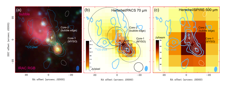
Figure 1.— (a) Overall structures of the binary G350.69-0.49 from the Spitzer and SMA observations. The background is the Color-synthesized image from the Spitzer/IRAC 3.6(blue), 4.5(green), 8.0(red) $\micron$ bands. The red emission in the 8.0 $\micron$ band highlights the hot gas Bubble illuminated by the central star; the 4.5 $\micron$ emission is largely contributed by the shock excited CO and H₂ emission, and thus may trace the interaction between the high-velocity gas flow and the surrounding gas. The blue contours represent the velocity integrated ¹³CO emission. The contour levels are 4, 10, 20, 30 times 0.75 Jy beam^-1 km s^-1.The thin white contours represent the 1.3 mm continuum emission which reveals two dense dust-and-gas cores located at the Bubble edge and the MYSO, respectively.The contour levels are 4, 10, 20, 30, 40, 50 times 0.003 Jy beam^-1. (b) The ¹³CO (2-1) and 1.3 mm continuum emissions overlaid on the Herschel/PACS 70 $\micron$ continuum image (gray scale). The two dashed circles represent the apertures to measure the flux density of Core-1 and the total flux density of Core-2+Bubble. (c) Same as (b) except for that the background image is the SPIRE 500 $\micron$ image.

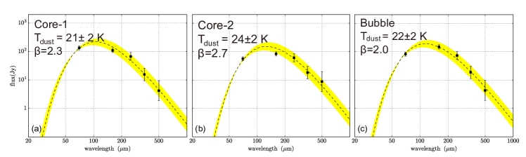
Figure 2.— The spectral energy distributions (SEDs) for the three objects. The apertures for measuring the flux densities are presented in Figure 1b. The yellow-shaded area represent the variation of the best-fit SED curve due to the flux uncertainties.

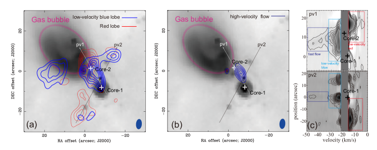
Figure 3.— Molecular gas kinematics of the G350.69-0.49 region from the SMA observations. (a) The ¹²CO low-velocity flow components in different velocity ranges. The cyan and red represent the low-velocity flow in (-32,-22) and (-16,-4) km s^-1 ranges, respectively. And the contour levels are 4, 10, 20, 30, 40 times 0.72 Jy beam^-1 km s^-1; the white crosses represent the location of the two dense cores. (b) The fast flow in the velocity interval of (-50,-32) km s^-1; the contour levels are 4, 6, 8, 10, 12 times 0.86 Jy beam^-1 km s^-1. (c) The position-velocity diagrams along the two directions labelled in the main panel, with the velocity range and the bulk spatial extent of the gas flows indicated by the colored boxes. The contour levels are from 0.5 K (0.27 Jy beam^-1) in step of 1 K.

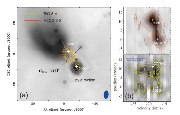
Figure 4.— (a) The velocity integrated emissions of the SiO (5-4) and H₂CO (3-2) lines overlaid on the IRAC 8 $\micron$ image. For both species, the contours are 4, 6, 8… times the rms level (0.5 Jy beam^-1 km s^-1). The diameter of the flow cross section $(d_{\rm flow})$ is measured and labeled on the figure. (b) the PV diagrams of the two lines along the velocity gradient over Core-1. The contour levels are 0.2 to 1.8 K in step of 0.2 K for SiO, and 0.3 to 5.1 K in step of 0.6 K for H₂CO.

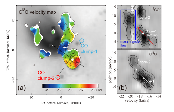
Figure 5.— (a) The velocity integrated emission of C¹⁸O (2-1) and its intensity-weighted velocity distribution (moment-1 map) overlaid on the IRAC 8 $\micron$ image. The contour levels are 4, 10, 20, 30, 40, 50 times the uncertainty level (0.5 Jy beam^-1 km s^-1). (b) the PV diagrams of the ¹³CO and C¹⁸O and (2-1) along the direction from Core-1 to Core-2. The contour levels are 0.5 to 3.0 K in step of 0.5 K for ¹³CO, and 0.8 to 5.3 K in step of 0.9 K for C¹⁸O.

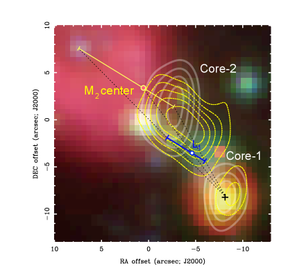
Figure 6.— The Lagrange L1 point between the two cores as calculated from a binary model using Equation (4). The uncertainty range is estimated by assuming the mass center of M2 (including Bubble and Core-2) varying from the Bubble center to Core-2 center, The two limits are represented by the error bars.

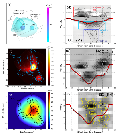
Figure 7.— The simplified gas structures modeling and the resultant velocity field purely due to the their overall gravity. (a) The 3D gas components used to model the observed gas morphologies. (b) The gas column density map overlaid on the observed ¹³CO image. (c) The velocity distribution calculated from Equation (8), assuming gas is infalling from the Bubble center, representing the maximum velocity that the can be reached (d)-(f) The modeled velocity distribution along the direction from Core-2 to Core-1 overlaid on the PV diagrams of ¹²CO, ¹³CO, and SiO lines, respectively.