Abstract
Models for fitting spatio-temporal point processes should incorporate spatio-temporal inhomogeneity and allow for different types of interaction between points (clustering or regularity). This paper proposes an extension of the spatial multi-scale area-interaction model to a spatio-temporal framework. This model allows for interaction between points at different spatio-temporal scales and the inclusion of covariates. We fit the proposed model to varicella cases registered during 2013 in Valencia, Spain. The fitted model indicates small scale clustering and regularity for higher spatio-temporal scales.

Keywords & Phrases: Gibbs point processes; multi-scale area-interaction model; spatio-temporal point processes; varicella.

2010 Mathematics Subject Classification: 60D05, 60G55, 62M30.

1 Introduction

Spatio-temporal patterns are increasingly observed in many different fields, including ecology, epidemiology, seismology, astronomy and forestry. The common feature is that all observed events have two basic characteristics: the location and the time of the event. Here we are mainly concerned with epidemiology [33], which studies the distribution, causes and control of diseases in a defined human population. The locations of the occurrence of cases give information on the spatial behavior of the disease, whereas the times, measured on different scales (days, weeks, years, period of times), give insights on the temporal response of the overall process. An essential point to take into consideration is that people are not uniformly distributed in space, hence information on the spatial distribution of the population at risk is crucial when analyzing spatio-temporal patterns of diseases.

Realistic models to fit epidemiological data should incorporate spatio-temporal inhomogeneity and allow for different types of dependence between points. One important class of such models is the family of Gibbs point processes, defined in terms of their probability density function [21, 28, 29], and, in particular, the sub-class of pairwise interaction processes. Well-known examples of pairwise interaction processes are the Strauss model [16, 36] or the hard core process, a particular case of the Strauss model where no points ever come closer to each other than a given threshold. However, pairwise interaction models are not always a suitable choice for fitting clustered patterns. A family of Markov point processes that can fit both clustered and ordered patterns is that of the area- or quermass-interaction models [2, 18]. These models are defined in terms of stochastic geometric functionals and display interactions of all orders. Methods for inference and perfect simulation are available in [10, 13, 17, 23].

Most natural processes exhibit interaction at multiple scales. The classical Gibbs processes model spatial interaction at a single scale, nevertheless multi-scale generalizations have been proposed in the literature [1, 12, 24]. In this paper we propose an extension of the spatial multi-scale area-interaction model to a spatio-temporal framework.

The outline of the paper is as follows. Section 2 provides some preliminaries in relation to notation and terminology. Section 3 gives the definition and Markov properties of our spatio-temporal multi-scale area-interaction model. Section 4 adapts simulation algorithms, such as the Metropolis-Hastings and the birth-and-death algorithms, to our context. Section 5 treats the pseudo-likelihood method for inference as well as an extension of the Berman-Turner procedure. The ideas are illustrated on a simulated example. The model is applied to a varicella data set in Section 6. Section 7 presents final remarks and a discussion of future work.

2 Preliminaries

A realization of a spatio-temporal point process consists of a finite number $n\geq 0$ of distinct points $(x_{i},t_{i})$, $i=1,\ldots,n$, that are observed within a compact spatial domain $W_{S}\subseteq{\mathbb{R}^{2}}$ and time interval $W_{T}\subseteq{\mathbb{R}}$. The pattern formed by the points will be denoted by ${\rm{\bf{x}}}=\{(x_{i},t_{i})\}_{i=1}^{n}$. For a mathematically rigorous account, the reader is referred to [8, 9].

We define the Euclidean norm $||x||=(x_{1}^{2}+x_{2}^{2})^{1/2}$ and the Euclidean metric $d_{{\mathbb{R}^{2}}}(x,y)=||x-y||$ for $x=(x_{1},x_{2})\in{\mathbb{R}^{2}}$ and $y=(y_{1},y_{2})\in{\mathbb{R}^{2}}$. We need to treat space and time differently, thus on ${\mathbb{R}^{2}\times\mathbb{R}}$ we consider the supremum norm $||(x,t)||_{\infty}=\max\{||x||,|t|\}$ and the supremum metric $d((x,t),(y,s))=||(x,t)-(y,s)||_{\infty}=\max\{||x-y||,|t-s|\}$, where $(x,t),(y,s)\in{\mathbb{R}^{2}\times\mathbb{R}}$. Note that $({\mathbb{R}^{2}\times\mathbb{R}},d(\cdot,\cdot))$ as well as its restriction to $W_{S}\times W_{T}$ is a complete, separable metric space. We write ${\mathcal{B}}({\mathbb{R}^{2}\times\mathbb{R}})={\mathcal{B}}({\mathbb{R}^{2}})\otimes{\mathcal{B}}({\mathbb{R}})$ for the Borel $\sigma$-algebra and $\ell$ for Lebesgue measure. We denote by $\oplus$ the Minkowski addition of two sets $A,B\subset{\mathbb{R}^{2}}$, defined as the set $A\oplus B=\{a+b:a\in A,b\in B\}$.

As stated in Section 1, Gibbs models form an important class of models able to fit epidemiological data exhibiting spatio-temporal inhomogeneity and interaction between points. In space, the Widom-Rowlinson penetrable sphere model [39] produces clustered point patterns; the more general area-interaction model [2] fits both clustered and inhibitory point patterns. In its most simple form, the area-interaction model is defined by its probability density

(1) $$p({\rm{\bf{x}}})=\alpha\lambda^{n({\rm{\bf{x}}})}\gamma^{-A({\rm{\bf{x}}})}$$

with respect to a unit rate Poisson process on $W_{S}$. Here $\alpha$ is the normalizing constant, ${\rm{\bf{x}}}$ is a spatial point configuration in $W_{S}\subset{\mathbb{R}^{2}}$, $n({\rm{\bf{x}}})$ is the cardinality of ${\rm{\bf{x}}}$ and $A({\rm{\bf{x}}})$ is the area of the union of discs of radius $r$ centered at $x_{i}\in{\rm{\bf{x}}}$ restricted to $W_{S}$. The positive scalars $\lambda$, $\gamma$ and $r>0$ are the parameters of the model. Note that, as emphasized in [21], Gibbsian interaction terms can be combined to yield more complex models. Doing so, [1, 12, 24] develop an extension of the area-interaction process which incorporates both inhibition and attraction. We propose a further generalization of the area-interaction model to allow multi-scale interaction in a spatio-temporal framework.

3 Space-time area-interaction processes

Let ${\rm{\bf{x}}}$ be a finite spatio-temporal point configuration on $W_{S}\times W_{T}\subset{\mathbb{R}^{2}\times\mathbb{R}}$, that is, a finite set of points, including the empty set.

Definition 1.

The spatio-temporal multi-scale area-interaction process is the point process with density

(2) $$p({\rm{\bf{x}}})=\alpha\prod_{(x,t)\in{\rm{\bf{x}}}}\lambda(x,t)\prod_{j=1}^{m}\gamma_{j}^{-\ell({\rm{\bf{x}}}\oplus G_{j})}$$

with respect to a unit rate Poisson process on $W_{S}\times W_{T}$, where $\alpha>0$ is a normalizing constant, $\lambda\geq 0$ is a measurable and bounded function, $\ell$ is Lebesgue measure restricted to $W_{S}\times W_{T}$, $\gamma_{j}>0$ are the interaction parameters, $G_{j}$ are some compact subsets of ${\mathbb{R}^{2}\times\mathbb{R}}$ with size depending on $j$, $j=1,\ldots,m$, $m\in\mathbb{N}$, and $\oplus$ denotes Minkowski addition.

Note that when ${\rm{\bf{x}}}$ is the empty set, $p({\rm{\bf{x}}})=\alpha$. The interaction parameters have the same interpretation as for the spatial area-interaction model (1). For fixed $j\in\{1,\ldots,m\}$, when $0<\gamma_{j}<1$ we would expect to see inhibition between points at spatio-temporal scales determined by the definition of the compact set $G_{j}$. On the other hand, when $\gamma_{j}>1$ we expect clustering between the points. We observe that (2) reduces to an inhomogeneous Poisson process when $\gamma_{j}=1$ for all $j\in\{1,\ldots,m\}$.

Covariates can be introduced in the model by letting the intensity function $\lambda$ be a measurable and bounded function $\lambda(x,t)=\rho(Z(x,t))$ of the covariate vector $Z(x,t)$.

The new model proposed in (2) successfully extends the area-interaction model to multi-scale interaction for spatio-temporal point patterns.

Lemma 1.

The density (2) is measurable and integrable for all $\gamma_{j}$, $j=1,\ldots,m$, $m\in\mathbb{N}$.

Proof.

Consider a point configuration, ${\rm{\bf{x}}}$. Since $\ell$ is $\sigma$-finite and $G_{j}$ is compact, the map ${\rm{\bf{x}}}\mapsto\ell({\rm{\bf{x}}}\oplus G_{j})$ is measurable for any $j=1,\ldots,m$. It follows that the map ${\rm{\bf{x}}}\mapsto\exp[-\ell({\rm{\bf{x}}}\oplus G_{j})\log{\gamma_{j}}]$ is measurable for any $j=1,\ldots,m$. The map ${\rm{\bf{x}}}\mapsto\prod_{x_{i}\in{\rm{\bf{x}}}}\lambda(x_{i},t_{i})$ is also measurable by assumption, hence the density (2) is measurable.

To determine if (2) is integrable, we observe that $0\leq\ell({\rm{\bf{x}}}\oplus G_{j})\leq\ell(W_{S}\times W_{T})<\infty$. The function $\lambda$ is integrable by assumption, hence (2) is dominated by an integrable function, and therefore integrable. ∎

As a further simplification, for fixed $j\in\{1,\ldots,m\}$, consider the case where ${\rm{\bf{x}}}\oplus G_{j}=\bigcup_{(x,t)\in{\rm{\bf{x}}}}\mathcal{C}_{r_{j}}^{t_{j}}(x,t)$ is the union of all cylinders with radius $(r_{j},t_{j})$ centered in $(x,t)$ taken over all $(x,t)\in{\rm{\bf{x}}}$. We define the cylinder with radius $(r_{j},t_{j})$ by

$$\mathcal{C}_{r_{j}}^{t_{j}}(x,t)=\{(y,s)\in W_{S}\times W_{T}:||x-y||\leq r_{j},|t-s|\leq t_{j}\}.$$

Then ${\rm{\bf{x}}}\oplus G_{j}$ is the set of all points within the cylinders $\mathcal{C}_{r_{j}}^{t_{j}}(x,t)$ centered in points of ${\rm{\bf{x}}}$ and the expression (2) reads

(3) $$p({\rm{\bf{x}}})=\alpha\prod_{(x,t)\in{\rm{\bf{x}}}}\lambda(x,t)\prod_{j=1}^{m}\gamma_{j}^{-\ell(\cup_{(x,t)\in{\rm{\bf{x}}}}\mathcal{C}_{r_{j}}^{t_{j}}(x,t))},$$

where $(r_{j},t_{j})$ are pairs of irregular parameters [4] of the model and $\gamma_{j}$ are interaction parameters, $j=1,\ldots,m$. The function $\lambda$ is here assumed known for simplicity, but could also depend on further parameters.

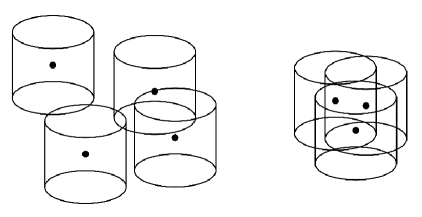
Figure 1: An illustration of possible ${\rm{\bf{x}}}\oplus G$ (cylinders around the points), where the black dots represent points of the process.

Figure 1 shows an illustration of ${\rm{\bf{x}}}\oplus G_{j}$. When $0<\gamma_{j}<1$, point configurations such as the one on the left are likely to be observed (inhibition between points), whereas for large $\gamma_{j}>1$, point configurations such as the one on the right are more likely to be observed (attraction between points).

3.1 Markov properties

Let $\sim$ on ${\mathbb{R}^{2}\times\mathbb{R}}$ be a symmetric and reflexive relation on ${\mathbb{R}^{2}\times\mathbb{R}}$, i.e. for any $(x,t),(y,s)\in{\mathbb{R}^{2}\times\mathbb{R}}$, $(x,t)\sim(y,s)\Leftrightarrow(y,s)\sim(x,t)$ and $(x,t)\sim(x,t)$. Two points $(x,t)$ and $(y,s)$ are said to be neighbors if $(x,t)\sim(y,s)$. An example of a fixed range relation on ${\mathbb{R}^{2}\times\mathbb{R}}$ is

(4) $$(x,t)\sim(y,s)\Leftrightarrow(x,t)\oplus G\cap(y,s)\oplus G\neq\emptyset,$$

where $G=\mathcal{C}_{r_{1}}^{t_{1}}$ is a cylinder of radius $(r_{1},t_{1})$.

Definition 2.

A point process has the Markov property [21, 30] with respect to the symmetric, reflexive relation $\sim$, if, for all point configurations ${\rm{\bf{x}}}$ with $p({\rm{\bf{x}}})>0$, the following conditions are fulfilled:

1. $p({\rm{\bf{y}}})>0$ for all ${\rm{\bf{y}}}\subseteq{\rm{\bf{x}}}$;

2. the likelihood ratio $\dfrac{p({\rm{\bf{x}}}\cup\{(y,s)\})}{p({\rm{\bf{x}}})}$ for adding a new point $(y,s)$ to a point configuration ${\rm{\bf{x}}}$ depends only on points $(x,t)\in{\rm{\bf{x}}}$ such that $(y,s)\sim(x,t)$, i.e. depends only on the neighbors of $(y,s)$.

Lemma 2.

The spatio-temporal multi-scale area-interaction process (2) is a Markov point process with respect to the relation (4) in the sense of [30].

Proof.

Note that if $p({\rm{\bf{x}}})>0$, since $\lambda(x,t)>0$ for all $(x,t)\in{\rm{\bf{x}}}$, then whenever ${\rm{\bf{y}}}\subseteq{\rm{\bf{x}}}$, also $p({\rm{\bf{y}}})>0$. The likelihood ratio

$$\dfrac{p({\rm{\bf{x}}}\cup\{(y,s)\})}{p({\rm{\bf{x}}})} =\dfrac{\alpha\displaystyle\left(\prod_{(x,t)\in{\rm{\bf{x}}}}\lambda(x,t)\right)\lambda(y,s)\displaystyle\prod_{j=1}^{m}\gamma_{j}^{-\ell(({\rm{\bf{x}}}\cup\{(y,s)\})\oplus G_{j})}}{\alpha\displaystyle\prod_{(x,t)\in{\rm{\bf{x}}}}\lambda(x,t)\displaystyle\prod_{j=1}^{m}\gamma_{j}^{-\ell({\rm{\bf{x}}}\oplus\it G_{j})}}$$

(5) $$=\lambda(y,s)\displaystyle\prod_{j=1}^{m}\displaystyle\gamma_{j}^{-\ell\left(((y,s)\oplus G_{j})\setminus({\rm{\bf{x}}}\oplus G_{j})\right)}.$$

Note that

$$((y,s)\oplus G_{j})\setminus({\rm{\bf{x}}}\oplus G_{j}) =((y,s)\oplus G_{j})\cap\left[\bigcup_{(x,t)\in{\rm{\bf{x}}}}(x,t)\oplus G_{j}\right]^{C}$$

$$=((y,s)\oplus G_{j})\cap\left[\bigcup_{(x,t)\sim(y,s)}(x,t)\oplus G_{j}\right]^{C},\quad\forall j=1,\ldots,m.$$

Thus (5) depends only on the newly added point $(y,s)$ and its neighbors. Hence (2) defines a Markov point process with respect to $\sim$. ∎

It follows that the density $p(\cdot)$ in (2) is Markov at range $2\max\{(r_{j},t_{j})\}$, $j=1,\ldots,m$.

Define the Papangelou conditional intensity of a point process with density $p$ by

$$\lambda((y,s);{\rm{\bf{x}}})=\dfrac{p({\rm{\bf{x}}}\cup\{(y,s)\})}{p({\rm{\bf{x}}})},$$

whenever $p({\rm{\bf{x}}})>0$ and $(y,s)\in{\rm{\bf{x}}}$. Then, for the spatio-temporal multi-scale area-interaction process, by the proof of Lemma 2 we obtain that

(6) $$\lambda((y,s);{\rm{\bf{x}}}) =\lambda(y,s)\displaystyle\prod_{j=1}^{m}\gamma_{j}^{-\ell(\mathcal{C}_{r_{j}}^{t_{j}}(y,s)\setminus\bigcup_{(x,t)\in{\rm{\bf{x}}}}\mathcal{C}_{r_{j}}^{t_{j}}(x,t))},$$

or, upon transformation to a logarithmic scale,

$$\log{\lambda((y,s);{\rm{\bf{x}}})} =\log{\lambda(y,s)}-\displaystyle\sum_{j=1}^{m}(\log{\gamma_{j}})\,\ell\left(\mathcal{C}_{r_{j}}^{t_{j}}(y,s)\setminus\bigcup_{(x,t)\in{\rm{\bf{x}}}}\mathcal{C}_{r_{j}}^{t_{j}}(x,t)\right).$$

Note that $\lambda(y,s)$ may be $0$, thus making $\log{\lambda(y,s)}$ ill-defined.

Write $\eta_{j}=\log{\gamma_{j}}$. Then, whenever well-defined,

$$\log{\lambda((y,s);{\rm{\bf{x}}})} =\log{\lambda(y,s)}-\displaystyle\sum_{j=1}^{m}\eta_{j}\int_{W_{S}\times W_{T}}{\mathbf{1}}\{(z,u)\in\mathcal{C}_{r_{j}}^{t_{j}}(y,s)\setminus\bigcup_{(x,t)\in{\rm{\bf{x}}}}\mathcal{C}_{r_{j}}^{t_{j}}(x,t)\}\,dz\,du$$

(7) $$=\log{\lambda(y,s)}-\displaystyle\sum_{j=1}^{m}\int_{\mathrm{F}_{r_{j}}^{t_{j}}(y,s)}\sum_{i=j}^{m}\eta_{i}\,{\mathbf{1}}\{(z,u)\notin\bigcup_{(x,t)\in{\rm{\bf{x}}}}\mathcal{C}_{r_{i}}^{t_{i}}(x,t)\}\,dz\,du,$$

where $\mathrm{F}_{r_{j}}^{t_{j}}\it(x,t)$ is the difference between two concentric cylinders $\mathcal{C}_{r_{j}}^{t_{j}}(x,t)$ and $\mathcal{C}_{r_{j-1}}^{t_{j-1}}(x,t)$.

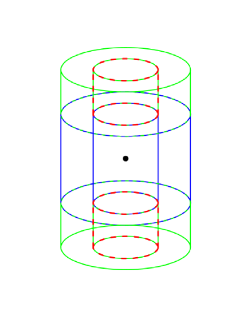
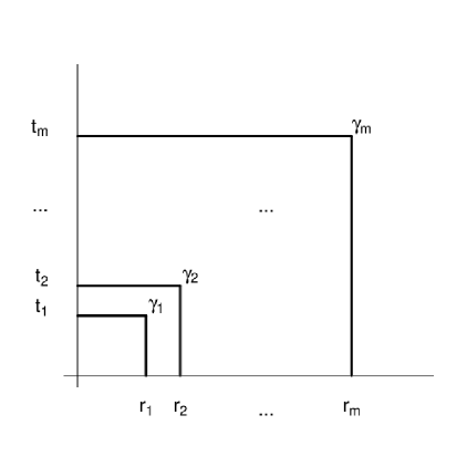
Figure 2: (Left) An illustration of $F_{r_{j}}^{t_{j}}$ where the blue annulus corresponds to $\{(y,s)\in W_{S}\times W_{T}:r_{j-1}<||x-y||\leq r_{j},|t-s|\leq t_{j-1}\}$, the two green annuli represent $\{(y,s)\in W_{S}\times W_{T}:r_{j-1}<||x-y||\leq r_{j},t_{j-1}<|t-s|\leq t_{j}\}$ and the two red cylinders are $\{(y,s)\in W_{S}\times W_{T}:||x-y||\leq r_{j-1},t_{j-1}<|t-s|\leq t_{j}\}$. (Right) Multi-scale behavior.

Indeed,

$$\mathrm{F}_{r_{j}}^{t_{j}}(x,t) = \mathcal{C}_{r_{j}}^{t_{j}}(x,t)\setminus\mathcal{C}_{r_{j-1}}^{t_{j-1}}(x,t)$$

$$= \left\{(y,s)\in W_{S}\times W_{T}:\begin{array}[]{l}r_{j-1}<||x-y||\leq r_{j},|t-s|\leq t_{j-1}\ \mathrm{or}\\ r_{j-1}<||x-y||\leq r_{j},t_{j-1}<|t-s|\leq t_{j}\ \mathrm{or}\\ ||x-y||\leq r_{j-1},t_{j-1}<|t-s|\leq t_{j}\end{array}\right\},$$

with $0=r_{0}<r_{1}<\cdots<r_{m}$ and $0=t_{0}<t_{1}<\cdots<t_{m}$. The left-most panel of Figure 2 shows an illustration of $F_{r_{j}}^{t_{j}}$ for fixed $r_{j},t_{j}$. The blue annulus corresponds to $\{(y,s)\in W_{S}\times W_{T}:r_{j-1}<||x-y||\leq r_{j},|t-s|\leq t_{j-1}\}$, the two green annuli represent $\{(y,s)\in W_{S}\times W_{T}:r_{j-1}<||x-y||\leq r_{j},t_{j-1}<|t-s|\leq t_{j}\}$ and the two red cylinders form $\{(y,s)\in W_{S}\times W_{T}:||x-y||\leq r_{j-1},t_{j-1}<|t-s|\leq t_{j}\}$. If, for $(y,s),||y-x||>2r_{m},|s-t|>2t_{m},\forall(x,t)\in{\rm{\bf{x}}}$, then

$$\log{\lambda((y,s);{\rm{\bf{x}}})} =\log{\lambda(y,s)}-\displaystyle\sum_{j=1}^{m}\left(\sum_{i=j}^{m}\eta_{i}\right)\ell(\mathrm{F}_{r_{j}}^{t_{j}}(y,s))$$

$$=\log{\lambda(y,s)}-\displaystyle\sum_{j=1}^{m}\eta_{j}\ell(C_{r_{j}}^{t_{j}}(y,s)).$$

To conclude this discussion, note that, in accordance with [12],

$$p({\rm{\bf{x}}})=\alpha\prod_{(x,t)\in{\rm{\bf{x}}}}\lambda(x,t)\,\exp{[-\sum_{j=1}^{m}\alpha_{j}\,\ell(F_{r_{j}}^{t_{j}}({\rm{\bf{x}}}))]},$$

where $\alpha_{j}=\sum_{i\geq j}\eta_{i}$ and $F_{r_{j}}^{t_{j}}({\rm{\bf{x}}}))=({\rm{\bf{x}}}\oplus G_{j})\backslash({\rm{\bf{x}}}\oplus G_{j-1})$ As before, $G_{j}=C_{r_{j}}^{t_{j}}$.

The model in (2) with Papangelou conditional intensity defined by (7) allows for models whose interaction behavior varies across spatio-temporal scales, for example, inhibition at small scales, attraction at larger scales and randomness beyond. The different spatio-temporal scales, $(r_{j},t_{j})$, are defined according to $\mathrm{F}_{r_{j}}^{t_{j}}$. Indeed, a point $(z,u)$ in $F_{r_{j}}^{t_{j}}({\rm{\bf{x}}})$ contributes a term $\alpha_{j}$ to the energy (the negative of the exponential term) in $p({\rm{\bf{x}}})$. The right-most panel of Figure 2 shows a visual representation of this multi-scale behavior.

An important property of Markov densities is the fact that the Papangelou conditional intensity, $\lambda((y,s);{\rm{\bf{x}}})$, depends only on $(y,s)$ and its neighbors in ${\rm{\bf{x}}}$, and is computationally convenient. This property will be exploited in the next section to design simulation algorithms for generating realisations of the model.

4 Simulation

4.1 The Metropolis-Hastings algorithm

Consider a Markov point process on $W_{S}\times W_{T}\subseteq{\mathbb{R}^{2}\times\mathbb{R}}$ defined by its density $p(\cdot)$. The Metropolis-Hastings algorithm, first introduced in statistical physics [5, 22], is a tool for constructing a Markov process with limit distribution defined by $p(\cdot)$.

Metropolis-Hastings algorithms are discrete time Markov processes where transitions are defined as the proposal of a new state that is accepted or rejected based on the likelihood of the proposed state compared with the old state. We consider two types of proposals: addition (birth) and deletion (death) of a point. The likelihood ratio of the new state in comparison with the old state, for these type of transitions, is the (reciprocal) conditional intensity.

More precisely, consider the point configuration ${\rm{\bf{x}}}$. We can propose either a birth or a death with respective probabilities $q({\rm{\bf{x}}})$ and $1-q({\rm{\bf{x}}})$ that depend on ${\rm{\bf{x}}}$. For a birth, a new point $u\in W_{S}\times W_{T}$ is sampled from a probability density $b({\rm{\bf{x}}},\cdot)$ and the new point configuration ${\rm{\bf{x}}}\cup\{u\}$ is accepted with probability $A({\rm{\bf{x}}},{\rm{\bf{x}}}\cup\{u\})$, otherwise the state remains unchanged, ${\rm{\bf{x}}}$. For a death, the point $x\in{\rm{\bf{x}}}$ chosen to be eliminated is selected according to a discrete probability distribution $d({\rm{\bf{x}}},\cdot)$ on ${\rm{\bf{x}}}$, and the proposal ${\rm{\bf{x}}}\setminus\{x\}$ is accepted with probability $A({\rm{\bf{x}}},{\rm{\bf{x}}}\setminus\{x\})$, otherwise the state remains unchanged.

In general, we can choose $b(\cdot,\cdot),d(\cdot,\cdot)$ and $q(\cdot)$ as we prefer. However, an important condition to consider is that of detailed balance, and therefore time-reversibility of the Markov process,

$$q({\rm{\bf{x}}})\,b({\rm{\bf{x}}},u)\,A({\rm{\bf{x}}},{\rm{\bf{x}}}\cup\{u\})\,p({\rm{\bf{x}}})=$$

(9) $$(1-q({\rm{\bf{x}}}\cup\{u\}))\,d({\rm{\bf{x}}}\cup\{u\},u)\,A({\rm{\bf{x}}}\cup\{u\},{\rm{\bf{x}}})\,p({\rm{\bf{x}}}\cup\{u\}).$$

For simplicity, consider the case that births and deaths are equally likely and sampled uniformly, that is, $q\equiv 1/2$, $b\equiv 1/\ell(W_{S}\times W_{T})$ and $d({{\rm{\bf{x}}}},\cdot)=1/n({\rm{\bf{x}}})$, where $n({\rm{\bf{x}}})$ is the number of points in the point configuration ${\rm{\bf{x}}}$. Then (4.1) reduces to

$$\dfrac{1}{2}\dfrac{1}{\ell(W_{S}\times W_{T})}{A({\rm{\bf{x}}},{\rm{\bf{x}}}\cup\{u\})\,p({\rm{\bf{x}}})} =\left(1-\dfrac{1}{2}\right)\dfrac{1}{n({{\rm{\bf{x}}}})+1}A({\rm{\bf{x}}}\cup\{u\},{\rm{\bf{x}}})\,p({\rm{\bf{x}}}\cup\{u\})$$

$$\dfrac{1}{\ell(W_{S}\times W_{T})}{A({\rm{\bf{x}}},{\rm{\bf{x}}}\cup\{u\})\,p({\rm{\bf{x}}})} =\dfrac{1}{n({{\rm{\bf{x}}}})+1}A({\rm{\bf{x}}}\cup\{u\},{\rm{\bf{x}}})\,p({\rm{\bf{x}}}\cup\{u\})$$

$$\dfrac{A({\rm{\bf{x}}},\ x\cup\{u\})}{A({\rm{\bf{x}}}\cup\{u\},{\rm{\bf{x}}})} =\underbrace{\dfrac{\ell(W_{S}\times W_{T})}{n({{\rm{\bf{x}}}})+1}\times\dfrac{p({\rm{\bf{x}}}\cup\{u\})}{p({\rm{\bf{x}}})}}_{=r({\rm{\bf{x}}},u)}.$$

Thus, more likely configurations can be favored by setting ${A({\rm{\bf{x}}},{\rm{\bf{x}}}\cup\{u\})}=\min\{1,r({\rm{\bf{x}}},u)\}$, and ${A({\rm{\bf{x}}}\cup\{u\},{\rm{\bf{x}}})}=\min\{1,1/r({\rm{\bf{x}}},u)\}$. Therefore, using equation (6), for the spatio-temporal multi-scale area-interaction process (2), the ratio $r({\rm{\bf{x}}},u)$ for $u=(y,s)$ reduces to

(10) $$r({\rm{\bf{x}}},u)=\dfrac{\ell(W_{S}\times W_{T})}{n({{\rm{\bf{x}}}})+1}\lambda(y,s)\displaystyle\prod_{j=1}^{m}\gamma_{j}^{-\ell(\mathcal{C}_{r_{j}}^{t_{j}}(y,s)\setminus\bigcup_{(x,t)\in{\rm{\bf{x}}}}\mathcal{C}_{r_{j}}^{t_{j}}(x,t))}.$$

In practice, we will use the logarithmic form of the conditional intensity as given in equation (7). When the region $W_{S}\times W_{T}$ is irregular we use rejection sampling to generate a point uniformly at random from $W_{S}\times W_{T}$.

4.2 Birth-and-death-processes

In this section we discuss methods for simulating (2) using birth-and-death processes [25]. The birth-and-death process is a continuous time Markov process where the transition from one state to another is given by either a birth or a death. A birth is the transition from a point configuration ${\rm{\bf{x}}}\in W_{S}\times W_{T}\subseteq{\mathbb{R}^{2}\times\mathbb{R}}$ to ${\rm{\bf{x}}}\cup\{u\}$ by adding the point $u\in W_{S}\times W_{T}$. A death is the transition from a point configuration ${\rm{\bf{x}}}$ to ${\rm{\bf{x}}}\setminus\{x\}$ by eliminating a point $x\in{\rm{\bf{x}}}$. We denote by $b({\rm{\bf{x}}},u)\,du$ the transition rate for a birth and by $d({\rm{\bf{x}}},x)$ the transition rate of a death. The total birth rate from ${\rm{\bf{x}}}$ is the integral

$$B({\rm{\bf{x}}})=\int_{W_{S}\times W_{T}}b({\rm{\bf{x}}},u)\,du$$

and the total death rate is

$$D({\rm{\bf{x}}})=\sum_{x\in{\rm{\bf{x}}}}d({\rm{\bf{x}}},x).$$

The process stays in state $X^{(n)}={\rm{\bf{x}}}$ for an exponentially distributed random sojourn time $T^{(n)}$ with mean $1/(B({\rm{\bf{x}}})+D({\rm{\bf{x}}}))$. The detailed balance equations are given by

(11) $$b({\rm{\bf{x}}},u)\,p({\rm{\bf{x}}})=d({\rm{\bf{x}}}\cup\{u\},u)\,p({\rm{\bf{x}}}\cup\{u\}).$$

We consider the particular case when the death rate is constant [27], $d({{\rm{\bf{x}}}},x)=1$. Hence, for the spatio-temporal multi-scale area-interaction process (2), the birth rate is given by the conditional intensity (cf. equation (6))

(12) $$b({\rm{\bf{x}}},(y,s))=\dfrac{p({\rm{\bf{x}}}\cup\{(y,s)\})}{p({\rm{\bf{x}}})}=\lambda(y,s)\displaystyle\prod_{j=1}^{m}\gamma_{j}^{-\ell(\mathcal{C}_{r_{j}}^{t_{j}}(y,s)\setminus\bigcup_{(x,t)\in{\rm{\bf{x}}}}\mathcal{C}_{r_{j}}^{t_{j}}(x,t))}.$$

For computation of the ratio in equation (12) we will use the logarithmic form of the conditional intensity as in equation (7).

Following [20, 21] we define an algorithm for simulating a birth-and-death process and generate the successive states $X^{(n)}$ and the sojourn times $T^{(n)}$ as detailed in Algorithm 1 which incorporates a rejection sampling step for computational convenience. Define a threshold $w({\rm{\bf{x}}})$, and, for $u\notin{\rm{\bf{x}}}$, set

$$g({\rm{\bf{x}}},u)=\begin{cases}b({\rm{\bf{x}}},u),&\text{if }b({\rm{\bf{x}}},u)\geq w({\rm{\bf{x}}})\\ w({\rm{\bf{x}}}),&\text{otherwise}.\end{cases}$$

A common choice is to take $w({\rm{\bf{x}}})$ equal to an upper bound to the conditional intensity.

Denote by $G({\rm{\bf{x}}})$ the integral of $g$. We generate the sequence of $(X^{(n)},T^{(n)})$ as follows.

Algorithm 1.

Initialize $X^{(0)}={\rm{\bf{x}}}_{0}$ for some finite point configuration with density function $p({\rm{\bf{x}}}_{0})>0$. For $n=0,1,\ldots$, if $X^{(n)}={\rm{\bf{x}}}$, compute $D=D({\rm{\bf{x}}})$, $G=G({\rm{\bf{x}}})$ and set $T^{(n)}=0$.

• Add an exponentially distributed time to $T^{(n)}$ with mean $1/(D+G)$;

• with probability $D/(D+G)$ generate a death $X^{(n+1)}={\rm{\bf{x}}}\setminus\{x\}$ by eliminating one of the current points $x\in{\rm{\bf{x}}}$ at random according to distribution $d(\cdot,\cdot)$ and stop;

• else sample a point $u$ from $g({\rm{\bf{x}}},u)/G$; with probability $b({\rm{\bf{x}}},u)/g({\rm{\bf{x}}},u)$ accept the birth $X^{(n+1)}={\rm{\bf{x}}}\cup\{u\}$ and stop; otherwise repeat the whole algorithm.

5 Inference

5.1 Pseudo-likelihood method

In this section, we assume that the function $\lambda$ is known and denote by $\theta=(\gamma_{1},\gamma_{2},\ldots,\gamma_{m})$ the interaction parameters in model (3). To estimate $\theta$, we may use pseudo-likelihood which aims to optimize

(13) $$PL({\rm{\bf{x}}},\theta)=\exp\left(-\int_{W_{S}}\int_{W_{T}}\lambda_{\theta}((u,v);{\rm{\bf{x}}})\,du\,dv\right)\prod_{(x,t)\in{\rm{\bf{x}}}}\lambda_{\theta}((x,t);{\rm{\bf{x}}}\setminus\{(x,t)\}),$$

where $\lambda_{\theta}((u,v);{\rm{\bf{x}}})$ is the conditional intensity that depends on $\theta$ [6].

For a Poisson process the conditional intensity is equal to the intensity function, hence pseudo-likelihood is equivalent to maximum likelihood. In general, the pseudo-likelihood $PL({\rm{\bf{x}}},\theta)$ is only an approximation of the true likelihood. However, no sampling is needed and the computational load will be considerably smaller than for the maximum likelihood method.

The maximum pseudo-likelihood normal equations are then given by

(14) $$\dfrac{\partial}{\partial\theta}\log PL({\rm{\bf{x}}},\theta)=0,$$

where

(15) $$\log PL({\rm{\bf{x}}},\theta)=\sum_{(x,t)\in{\rm{\bf{x}}}}\log\lambda_{\theta}((x,t);{\rm{\bf{x}}}\setminus\{(x,t)\})-\int_{W_{S}}\int_{W_{T}}\lambda_{\theta}((u,v);{\rm{\bf{x}}})\,du\,dv.$$

As seen in Section 3.1, the Papangelou conditional intensity of the spatio-temporal multi-scale area-interaction model is

$$\lambda_{\theta}((y,s);{\rm{\bf{x}}})=\lambda(y,s)\displaystyle\prod_{j=1}^{m}\gamma_{j}^{-\ell(\mathcal{C}_{r_{j}}^{t_{j}}(y,s)\setminus\cup_{{\rm{\bf{x}}}}^{j})},$$

where $\cup_{{\rm{\bf{x}}}}^{j}=\bigcup_{(x,t)\in{\rm{\bf{x}}}}\mathcal{C}_{r_{j}}^{t_{j}}(x,t)$; its logarithm reads

$$\log{\lambda_{\theta}((y,s);{\rm{\bf{x}}})} =\log{\lambda(y,s)}-\displaystyle\sum_{j=1}^{m}(\log{\gamma_{j}})\,\ell(\mathcal{C}_{r_{j}}^{t_{j}}(y,s)\setminus\cup_{{\rm{\bf{x}}}}^{j}).$$

Following [3] we denote by $S_{j}(y,s)=\ell(\mathcal{C}_{r_{j}}^{t_{j}}(y,s)\setminus\cup_{{\rm{\bf{x}}}}^{j})$ the sufficient statistics, hence $\log{\lambda_{\theta}((y,s);{\rm{\bf{x}}})}=\log\lambda(y,s)-\theta^{T}\begin{bmatrix}S_{1}(y,s)\\ \cdots\\ S_{m}(y,s)\end{bmatrix}$. This notation will be further used in Algorithm 2.

Thus, equation (14) gives us the pseudo-likelihood equations

$$\dfrac{\partial}{\partial\theta}\big{(}\sum_{(x,t)\in{\rm{\bf{x}}}} \left[\log{\lambda(x,t)}-\displaystyle\sum_{j=1}^{m}(\log{\gamma_{j}})\,\ell(\mathcal{C}_{r_{j}}^{t_{j}}(x,t)\setminus\cup_{{\rm{\bf{x}}}\setminus\{(x,t)\}}^{j})\right]-$$

(16) $$-\int_{W_{S}}\int_{W_{T}}\lambda(u,v)\displaystyle\prod_{j=1}^{m}\gamma_{j}^{-\ell(\mathcal{C}_{r_{j}}^{t_{j}}(u,v)\setminus\cup_{{\rm{\bf{x}}}}^{j})}\,du\,dv\big{)}=0.$$

For every parameter $\gamma_{i}$, $i=1,2,\ldots,m$, the equations (5.1) read

(17) $$\sum_{(x,t)\in{\rm{\bf{x}}}}\dfrac{\ell(\mathcal{C}_{r_{i}}^{t_{i}}(x,t)\setminus\cup_{{\rm{\bf{x}}}\setminus\{(x,t)\}}^{i}))}{\gamma_{i}}=\int_{W_{S}}\int_{W_{T}}\lambda(u,v)\dfrac{\ell(\mathcal{C}_{r_{i}}^{t_{i}}(u,v)\setminus\cup_{{\rm{\bf{x}}}}^{i})}{\gamma_{i}}\prod_{j=1}^{m}\gamma_{j}^{-\ell(\mathcal{C}_{r_{j}}^{t_{j}}(u,v)\setminus\cup_{{\rm{\bf{x}}}}^{j})}\,du\,dv.$$

The major difficulty is to estimate the integrals on the right hand side of equations (17). Baddeley and Turner [3] propose using the Berman-Turner method to approximate the integral in (15) by

$$\int_{W_{S}}\int_{W_{T}}\lambda_{\theta}((u,v);{\rm{\bf{x}}})\,du\,dv\approx\sum_{j=1}^{n}\lambda_{\theta}((u_{j},v_{j});{\rm{\bf{x}}})\,w_{j},$$

where $(u_{j},v_{j})$ are points in $W_{S}\times W_{T}$ and $w_{j}$ are quadrature weights. This yields an approximation for the log pseudo-likelihood of the form

(18) $$\log PL({\rm{\bf{x}}},\theta)\approx\sum_{(x,t)\in{\rm{\bf{x}}}}\log\lambda_{\theta}((x,t);{\rm{\bf{x}}}\setminus\{(x,t)\})-\sum_{j=1}^{n}\lambda_{\theta}((u_{j},v_{j});{\rm{\bf{x}}})\,w_{j}.$$

Note that if the set of points $\{(u_{j},v_{j}),j=1,\ldots,n\}$ includes all the points $(x,t)\in{\rm{\bf{x}}}$, we can rewrite (18) as

(19) $$\log PL({\rm{\bf{x}}},\theta)\approx\sum_{j=1}^{n}(y_{j}\log\lambda_{j}-\lambda_{j})\,w_{j},$$

where $\lambda_{j}=\lambda_{\theta}((u_{j},v_{j});{\rm{\bf{x}}}\setminus\{(u_{j},v_{j})\})$, $y_{j}=z_{j}/w_{j}$ and

(20) $$z_{j}=\begin{cases}1,&\text{if }(u_{j},v_{j})\in{\rm{\bf{x}}}\ (\mathrm{is\ a\ point}),\\ 0,&\text{if }(u_{j},v_{j})\notin{\rm{\bf{x}}}\ (\mathrm{is\ a\ dummy\ point}).\end{cases}$$

The right hand side of (19), for fixed ${\rm{\bf{x}}}$, is formally equivalent to the log-likelihood of independent Poisson variables $Y_{j}\sim\mathrm{Poisson}(\lambda_{j})$ taken with weights $w_{j}$. Therefore (19) can be maximized using software for fitting generalized linear models.

In summary, the method is as follows.

Algorithm 2.

• Generate a set of dummy points and merge them with all the data points in ${\rm{\bf{x}}}$ to construct the set of quadrature points $(u_{j},v_{j})\in W_{S}\times W_{T}$;

• compute the quadrature weights $w_{j}$;

• obtain the indicators $z_{j}$ defined in (20) and calculate $y_{j}=z_{j}/w_{j}$;

• compute the values $S_{j}(u_{j},v_{j})$ of the sufficient statistics at each quadrature point;

• fit a generalized log-linear Poisson regression model with parameters $\log\lambda_{j}$ given by $\log\lambda(u_{j},v_{j})-\theta^{T}S(u_{j},v_{j})$, responses $y_{j}$ and weights $w_{j}$.

The coefficient estimates returned by Algorithm 2 give the maximum pseudo-likelihood estimator $\hat{\theta}$ for $\theta$.

In order to estimate the parameters $\theta=(\gamma_{1},\gamma_{2},\ldots,\gamma_{m})$ using the above method we need to have values for the irregular parameters $r_{j}$ and $t_{j}$ for $j=1,\ldots,m$. Baddeley and Turner [3] suggest fitting the model for a range of values of these parameters and choose the values which maximize the pseudo-likelihood. Additionally, we recommend to first compute some summary statistics, such as the pair correlation or auto-correlation function, to narrow down the search.

We construct the quadrature scheme as a partition of $W_{S}\times W_{T}$ dividing the spatio-temporal area into cubes $C_{k}$ of equal volume. In the center of each cube $C_{k}$ we place exactly one dummy point. We then assign to each dummy or data point $(u_{j},v_{j})$ a weight $w_{j}=v/n_{j}$ where $v$ is the volume of each cube, and $n_{j}$ is the number of points, dummy or data, in the same cube as $(u_{j},v_{j})$. These weights are called the counting weights [3].

We conclude this section by mentioning briefly an alternative way to define the quadrature scheme (Algorithm 2). Indeed, [3] suggest the use of a Dirichlet tessellation to generate the quadrature weights. A quadrature scheme generated this way would mean that the weight of each point would be equal to the volume of the corresponding Dirichlet 3-dimensional cell. The computational cost of such a method is very high. Therefore, in this paper, we partition $W_{S}\times W_{T}$ into cubes of equal volume, as described above.

5.2 Simulation and parameter estimation of a spatio-temporal area interaction process

For illustration purposes, we simulate two multi-scale spatio-temporal area interaction processes as defined in (3), one which exhibits small scale inhibition and large scale clustering (simulation 1) and a second one which exhibits small scale clustering and large scale inhibition (simulation 2).

We consider the spatio-temporal domain $W_{S}\times W_{T}=([0,1]\times[0,1])\times[0,1]$ and in both cases take constant $\lambda\equiv 50$. For the irregular parameters we choose the same spatio-temporal scales $r_{1}=0.03$, $r_{2}=0.05$, $t_{1}=0.03$ and $t_{2}=0.05$ for both simulations. We use the Metropolis-Hastings algorithm described in Section 4.1 with $20,000$ iterations implemented in the MPPLIB C++ library [35]. To estimate the parameters we follow the steps in Algorithm 2. We partition $W_{S}\times W_{T}$ into $10^{3}=1,000$ cubes of volume $10^{-3}$. In the center of each cube we place a dummy point, obtaining a total of $1,000$ dummy points. We then compute the sufficient statistics for each data and dummy point using the MPPLIB C++ library and apply Algorithm 2 to obtain the estimates for the parameters. For the implementation of the pseudo-likelihood method we use the statistical software R [26] together with the spatstat [4] package. The theoretical background for computing the ‘envelopes’, that is the confidence interval bounds given as $2.5\%$ and $97.5\%$ in Tables 1 and 2 for a Poisson process is exhaustively described in [19].

Figure 3 (top left) shows the interaction parameters for simulation 1, $2\pi r_{1}^{2}t_{1}\log(\gamma_{1})=-5$ and $2\pi r_{2}^{2}t_{2}\log(\gamma_{2})=5$. This setting of parameters gives us the spatio-temporal point configuration shown in the top right panel of Figure 3 which indeed shows small scale inhibition between points and large scale clustering. The parameters estimates are shown in Table 1.

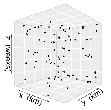
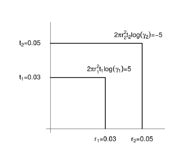
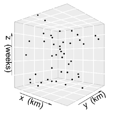
Figure 3: (Top left) Model parameters for simulation 1. (Top right) A realization of the first model. (Bottom left) Model parameters for simulation 2. (Bottom right) A realization of the second model.

	Estimate	2.5 %	97.5 %
$\log\lambda$	6.07	3.57	8.02
$2\pi r_{1}^{2}t_{1}\log(\gamma_{1})=-5$	-2.45	-5.48	0.37
$2\pi r_{2}^{2}t_{2}\log(\gamma_{2})=5$	4.48	2.44	6.48

Table 1: Parameter estimates for simulation 1.

For simulation 2 we choose interaction parameters $2\pi r_{1}^{2}t_{1}\log(\gamma_{1})=5$ and $2\pi r_{2}^{2}t_{2}\log(\gamma_{2})=-5$, as shown in the bottom left panel of Figure 3. The bottom right panel of Figure 3 shows a realization of the process with these parameters. We observe small scale clustering and large scale inhibition between points. The estimates of the parameters are given in Table 2.

Note that Figure 3 and Tables 1–2 correspond to a single realization of the multi-scale area-interaction model and one should be hesitant to draw any conclusions on the efficacy or otherwise of the pseudo-likelihood method from this illustration.

	Estimate	2.5 %	97.5 %
$\log\lambda$	8.25	4.56	10.50
$2\pi r_{1}^{2}t_{1}\log(\gamma_{1})=5$	7.17	2.69	12.00
$2\pi r_{2}^{2}t_{2}\log(\gamma_{2})=-5$	-2.39	-6.40	1.19

Table 2: Parameter estimates for simulation 2.

6 Data. Varicella in Valencia

The Varicella-zoster virus (VZV) is a highly contagious virus, spread worldwide, which causes two clinical syndromes: varicella, also known as chickenpox, and herpes zoster, otherwise known as shingles. In this paper we will focus on the spatial, temporal and spatio-temporal behavior of varicella.

Varicella is transmitted from person to person by direct contact with the rash or inhalation of aerosolized droplets from respiratory tract secretions of patients with varicella. In temperate countries more than $90\%$ of the infections occur before adolescence and less than $5\%$ of adults remain susceptible. Varicella is mostly a mild disorder in childhood, but tends to be more severe in adults. The first symptoms of varicella generally appear after a $10$ to $21$ days incubation period. It is characterized by an itchy, vesicular rash, fever and malaise. Varicella is generally self-limited and vesicles gradually develop crusts. It usually takes about $7$ to $10$ days for all the vesicles to dry out and for the crusts to disappear. This gives us a time period, from infection to completely dried vesicles, between $17$ and $31$ days.

Reported infection after household exposure ranges from $61\%$ to $100\%$ [11, 37] which indicates small range interaction. The disease may be fatal, especially in neonates and immuno-compromised individuals. The epidemiology of the disease is different in temperate and tropical climates. The reasons behind this behavior may be related to climate, population density and risk of exposure [14, 38].

In this paper we analyze varicella cases registered in Valencia, Spain, during 2013. Valencia is the third largest city in Spain with a population of around $800,000$ inhabitants in the administrative center ($19$ districts) and an area of approximately $134$ km² [34]. The study area is represented by districts $1$ to $16$. The remaining districts are very sparsely populated and are located far from the urban core. During the year 2013, $921$ cases of varicella were registered in the study area in the course of $52$ weeks [14].

The spatial coordinates of the varicella cases are expressed in latitude and longitude. First we transform them from longitude/latitude to UTM scale expressed in meters [31]. We then re-scale the spatial coordinates to kilometers such that the spatial study area reduces to $[0,9]\times[0,9]$. The temporal component of the process takes values from $0$ to $51$. For computational purposes to be explained later, we take the interval $[0,52]$ as the time window. Therefore, we set the spatio-temporal study area to $W_{S}\times W_{T}=([0,9]\times[0,9])\times[0,52]$ (km${}^{2}\times$ weeks). The spatio-temporal pattern of all varicella cases thus obtained is shown in Figure 4. The $x$- and $y$-axis represent the spatial coordinates in kilometers and the $z$-axis represents the time component in weeks.

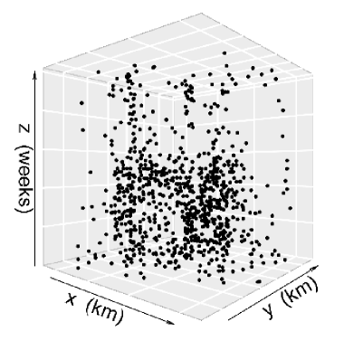
Figure 4: Spatio-temporal pattern of weekly varicella cases in Valencia during 2013, where the spatio-temporal study area is $W_{S}\times W_{T}=([0,9]\times[0,9])\times[0,52]$ (km${}^{2}\times$ weeks).

The main focus of our varicella data analysis is to quantify the interactions across a range of spatio-temporal scales. We do so by using the spatio-temporal multi-scale area-interaction model introduced in Section 3.

First we need to get some idea about a plausible upper bound to the values of the irregular parameters $(r_{j},t_{j})$, $j=1,\ldots,m$, in model (3). To this end, we use summary statistics for the spatial and temporal projections of the space-time point pattern shown in Figure 4.

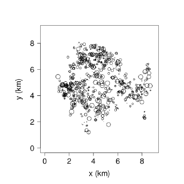
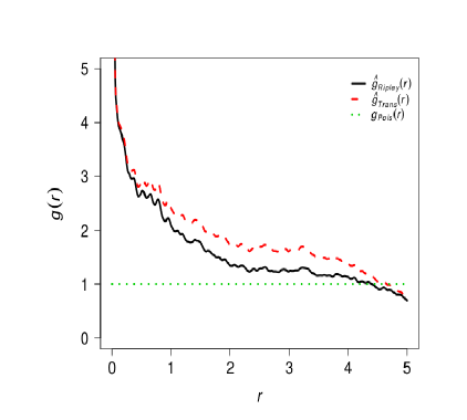
Figure 5: (Left) Spatial projection of the spatio-temporal point pattern for the varicella data. After projection, locations were jittered using a maximum jitter distance of $20$ metres. (Right) Estimated pair correlation function for the jittered spatial point pattern shown in the left panel.

The left panel in Figure 5 shows the projection of all points onto the spatial region. The sizes of the circles are proportional to time, the bigger the circle, the more recent the event. Due to the projection, duplicate locations are observed, so we jitter the coordinates uniformly on the spatial region around the duplicated points using a maximum jittering distance of $20$ meters. To get a rough indication of the spatial interaction range, we pretend that the pattern is stationary and isotropic, and estimate the pair correlation function. The result is shown in the right panel of Figure 5. Recall that for a Poisson process the pair correlation function is equal to $1$. Values of the pair correlation function lower than $1$ indicate inhibition and values larger than $1$ suggest clustering. Figure 5 suggests that the pair correlation function is approximately constant from $2$ kilometers onward, which indicates a maximum value for the $r_{i}$ of around $1$ kilometer. On a cautionary note, we need to keep in mind that the estimator only takes into account the spatial pattern of points and assumes isotropy.

The left panel in Figure 6 shows the temporal evolution of varicella over the $52$ weeks, where the small circles $\circ$ represents the number of registered cases. The right panel displays the estimated auto-correlation function which measures the correlation between the values of the series at different times as a function of the time lag between them. Figure 6 suggests possible correlation for time lags as big as $15$ weeks. This gives us an estimate for the maximum value for the $t_{i}$ of about $7.5$ weeks. Note that caveats similar to the spatial case apply.

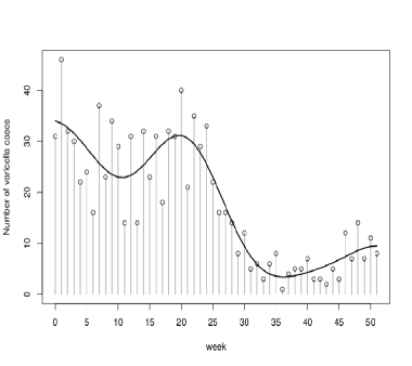
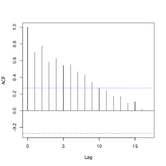
Figure 6: (Left) Weekly reports of varicella cases ($\circ$) and fitted regression curve (–). (Right) Estimated auto-correlation function for the data shown in the left panel.

Now that we have estimated the maximum spatial and temporal range for the model, the following step in our analysis is to consider covariate information. The most important factor in the transmission of any kind of disease, and especially a highly contagious one such as varicella, is the population. In areas with very low population we will probably not register as many varicella cases as in highly populated areas. Thus, the pattern of varicella cases can drastically change from one area to another, depending on the spatial distribution of the population, and from one week to the next one. We express the spatio-temporal inhomogeneity term in equation (3) as a product $\lambda(x,t)=\lambda(x)\,Z(t)$, $x\in[0,9]^{2}$, $t\in\{0,\ldots,51\}$, between a non-parametric estimate of the population density $\lambda(x)$ and a re-scaled parametric estimate of the temporal component $Z(t)$.

First consider the spatial component $\lambda(x)$. The population data available to us consist of the number of people living in each census section of the city of Valencia, a total number of $559$ sections (districts $1$ to $16$). We randomly generate within each section $p$ points, where $p$ is equal to the number of people living in that particular section. This way, we obtain a sample of the population for the city of Valencia. We estimate its intensity by a kernel estimator, keeping in mind that the bandwidth has to be chosen carefully, to get $\lambda(x)$, $x\in W_{S}$.

Following [15] we fit a harmonic regression to the pattern of the weekly varicella counts

(21) $$Z(t)=c_{0}+\sum_{j=1}^{3}\left(c_{j}\cos(2\pi jt/52)+d_{j}\sin(2\pi jt/52)\right)+c(a+bt),$$

where $Z(t)$ denotes the number of varicella cases at time $t$, $t=0,\ldots,51$, and $c_{0},a,b,c$, $c_{j},d_{j}$, $j=1,2,3$, are the parameters of the model.

The left panel in Figure 6 shows the fitted regression curve. We observe a period at the beginning of the year, from winter until spring, with large numbers of varicella cases, and a second period starting around week $26$, in which the number of cases decreases. These periods correspond roughly with the school term and the summer break. Also, in 2013, in Spain, there were several holidays besides the summer and winter holidays. On March 19, San Jose is celebrated and the period from the 24th to the 31st of March corresponds to the Easter holidays. As a consequence we can observe in Figure 6 a decrease during the 11th and 12th week. Towards the end of the year, the number of cases picks up again as the Michaelmas term begins.

Finally, we re-scale the parametric estimate of the temporal component $Z(t)$ by $100$, in order to avoid obtaining extreme values for the spatio-temporal inhomogeneity term $\lambda(x,t)$.

Since realizations of (3) do not contain points with equal time stamps, we jitter in time as well as space. More precisely, the week index is replaced by a time stamp that is uniformly distributed in the indicated week so that the temporal component falls in $W_{T}=[0,52]$. To estimate the parameters, we follow the steps described in Algorithm 2. For constructing the quadrature points we partition $W_{S}\times W_{T}$ into $9\times 9\times 52=4,212$ cubes of equal volume $1$ and place one dummy point in the center of each cube. Doing so, we obtain a total of $5,133$ dummy and data points. We attribute to each point a weight equal to the volume of the cube divided by the number of dummy and data points inside the cube containing the point. We then compute the sufficient statistics $S_{j}(\cdot,\cdot)$ corresponding to each point using the MPPLIB C++ library of [35]. We follow Algorithm 2 and obtain estimates for the parameters $\gamma$. The analysis and visual representations have been carried out using the statistical software R [26] together with the spatstat [4], plot3D [32] and rgdal [7] packages.

Recall that we found indications for the maximum spatial range to be about $2$ kilometers, the maximum temporal range $15$ weeks. As suggested in [3] we fitted the model for a range of values $(r_{j},t_{j})$, $j=1,\dots,m$, in the larger domain $[0,2]\times[0,15]$ and for different $m\in\{3,4,5,6,7,8\}$ to choose the optimal combination.

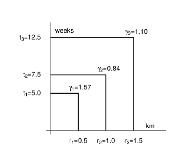
Figure 7: Model parameters for the varicella data.

We estimate $m=3$, that is, three spatio-temporal scales and the corresponding parameters. For the spatial scales we selected $r_{1}=0.5,r_{2}=1$ and $r_{3}=1.5$ kilometers and for the temporal scales $t_{1}=5$, $t_{2}=7.5$ and $t_{3}=12.5$ weeks. Figure 7 shows the multi-scale interaction in the data together with the estimated values of the model parameters. Also, Table 3 shows the estimated parameters of the model together with a confidence interval.

	Spatial scale	Temporal scale	Parameters	2.5%	97.5%
(Intercept)			1.20	1.09	1.31
	0.5	5.0	1.57	1.39	1.78
	1.0	7.5	0.84	0.74	0.95
	1.5	12.5	1.10	1.00	1.23

Table 3: Parameter estimates for the varicella data.

As stated before, the time period from infection to completely dried vesicles is between approximately $17$ and $31$ days. In the fitted model we observe that for a spatial lag of $0.5$ kilometer and a temporal lag of $5$ weeks there is clustering (significant $\gamma_{1}=1.57$). This means that for a period of five weeks and at rather small distance (as far as $0.5$ kilometers), a phenomenon of aggregation is observed between cases of varicella. The time lag corresponds more or less with the period of $31$ days indicated by the epidemiologists. This is caused by the main feature of chickenpox, being a contagious disease.

The fitted model also exhibits inhibition for spatial lags as far as $1$ kilometer and temporal lags up to $7.5$ weeks (significant $\gamma_{2}=0.84$). This might be a result of the fact that after recovery from varicella, patients usually have lifetime immunity. For higher spatial and temporal lags the model suggests no interaction ($\gamma_{3}\approx 1$), which corresponds with the rough bounds we found before and is in accordance with the beliefs of the epidemiologists. If you are situated far away from a varicella case, both in space and in time, you are less susceptible to contract the disease due to the contagious factor. Also, the probability of contracting the disease would be the same as the incidence of varicella.

To validate our model, we simulated a number of space-time multi-scale area-interaction processes with the fitted parameters using the Metropolis-Hastings algorithm described in Section 4.1 for $20,000$ iterations, which seems enough for the algorithm to converge based on diagnostic plots. Figure 8 shows one such simulation. Comparing Figure 4 and 8, we note that the simulated spatio-temporal point pattern is similar to the varicella point pattern.

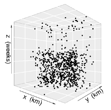
Figure 8: Realization from the model fitted to the varicella data.

7 Discussion and final remarks

In this paper we developed an extension of the area-interaction model that is able to incorporate different types of interaction at different spatio-temporal scales and proposed methods to simulate this process. We discussed inference and demonstrated the pseudo-likelihood method on simulated data. Additionally, we analyzed a spatio-temporal point pattern of varicella in the city of Valencia, Spain. For future work, it would be interesting to apply our model to other diseases that may exhibit interaction at several scales in space and time. It would also be very interesting to apply this model to data that are not necessarily related to epidemiology. Earthquake patterns, for instance, tend to show aggregation but also inhibition at different scales. Indeed, we believe that the proposed model may find applications in a wide range of research fields, such as forestry, geology and sociology.

As stated in Section 6, varicella is a highly infectious disease. We are certain that, in addition to the effect of the population, there are other covariates that may influence the spatio-temporal behavior of the disease. Therefore, an important goal for future work is to consider adding covariates that can improve the model. For example, [38] suggests that there are some climatic factors that can influence the epidemiology of varicella. Thus, covariates such as the monthly average temperatures, weekly average levels of rainfall, average hours of sunshine, or other climate related covariates, may provide useful information to the analysis of varicella. Also, additional information on the composition of households, income per capita or other socio-economical covariates might improve the model. Another important covariate that could be taken into account in future work is related to the locations of kindergartens, schools and high-schools: The distance from a case to the nearest school may provide important information for the analysis of varicella.

8 Software

Software in the form of R code and complete documentation are available on request from the corresponding author (iftimi@uv.es).

References

- [1] G. K. Ambler and B. W. Silverman. Perfect simulation using dominated coupling from the past with application to area-interaction point processes and wavelet thresholding. In: N. H. Bingham and C. M. Goldie (Eds.), Probability and Mathematical Genetics. Cambridge: Cambridge University Press, 2010.
- [2] A. J. Baddeley and M. N. M. van Lieshout. Area-interaction point processes. Annals of the Institute of Statistical Mathematics, 47:601–619, 1995.
- [3] A. Baddeley and R. Turner. Practical maximum pseudolikelihood for spatial point patterns (with discussion). Australian and New Zealand Journal of Statistics, 42:283–322, 2000.
- [4] A. Baddeley, E. Rubak and R. Turner. Spatial Point Patterns: Methodology and Applications with R. Boca Raton: Chapman and Hall/CRC Press, 2015.
- [5] A. A. Barker. Monte Carlo calculation of radial distribution functions for a proton-electron plasma. Australian Journal of Physics, 18:119–133, 1965.
- [6] J. E. Besag. Some methods of statistical analysis for spatial data. Bulletin of the International Statistical Institute, 47:77–92, 1975.
- [7] R. Bivand, T. Keitt and B. Rowlingson. Rgdal: Bindings for the Geospatial Data Abstraction Library, R package version 1.1-10, 2016.
- [8] D. J. Daley and D. Vere-Jones. An Introduction to the Theory of Point Processes. Volume I: Elementary Theory and Methods. (Second edition). New York: Springer-Verlag, 2003.
- [9] D. J. Daley and D. Vere-Jones. An Introduction to the Theory of Point Processes. Volume II: General Theory and Structure. New York: Springer-Verlag, 2008.
- [10] D. Dereudre, F. Lavancier and K. Staňková Helisová. Estimation of the intensity parameter of the germ-grain quermass-interaction model when the number of germs is not observed. Scandinavian Journal of Statistics, 41:809–829, 2014.
- [11] A. Gershon, M. Takahashi and J. Seward. Vaccines. (Fifth edition). Philadelphia: W. B. Saunders, 2008.
- [12] P. Gregori, M. N. M. van Lieshout and J. Mateu. Modelización de procesos area-interacción generalizados. (In Spanish). In: Proceedings 27 Congreso Nacional de Estadística e Invesigación Operativa, 2003.
- [13] O. Häggström, M. N. M. van Lieshout and J. Møller. Characterization results and Markov chain Monte Carlo algorithms including exact simulation for some spatial point processes. Bernoulli, 5:641–658, 1999.
- [14] Health Department. Varicella Report. Epidemiological Surveillance 2013. Public Health. Epidemiology and Health Surveillance. Epidemiological Surveillance and Control, May 2014.
- [15] A. Iftimi, F. Martínez-Ruiz, F. Míguez Santiyán and F. Montes. Spatio-temporal cluster detection of chickenpox in Valencia, Spain, 2008-2012. GeoSpatial Health, 10:54–62, 2015.
- [16] F. P. Kelly and B. D. Ripley. A note on Strauss’s model for clustering. Biometrika, 63:357–360, 1976.
- [17] W. S. Kendall. Perfect simulation for the area-interaction point process. In: L. Accardi and C. C. Heyde (Eds.), Probability Towards 2000. New York: Springer-Verlag, Lecture Notes in Statistics 128, 1998.
- [18] W. S. Kendall, M. N. M. van Lieshout and A. J. Baddeley. Quermass-interaction processes: Conditions for stability. Advances in Applied Probability, 31:315–342, 1999.
- [19] Y. A. Kutoyants. Statistical Inference for Spatial Poisson Processes. New York: Springer-Verlag, Lecture Notes in Statistics 134, 1998.
- [20] M. N. M. van Lieshout. Stochastic Geometry Models in Image Analysis and Spatial Statistics. Amsterdam: CWI Tract 108, 1995.
- [21] M. N. M. van Lieshout. Markov Point Processes and their Applications. London: Imperial College Press, 2000.
- [22] N. Metropolis, A. W. Rosenbluth, M. N. Rosenbluth and A. H. Teller. Equation of state calculations by fast computing machines. Journal of Chemical Physics, 21:1087–1092, 1953.
- [23] J. Møller and K. Helisová. Likelihood inference for unions of interacting discs. Scandinavian Journal of Statistics, 3:365–381, 2010.
- [24] N. Picard, A. Bar-Hen, F. Mortier and J. Chadœuf. The multi-scale marked area-interaction point process: A model for the spatial pattern of trees. Scandinavian Journal of Statistics, 36:23–41, 2009.
- [25] C. J. Preston. Spatial birth-and-death processes. Bulletin of the International Statistical Institute, 46:371–391, 1977.
- [26] R Core Team. R: A Language and Environment for Statistical Computing. R Foundation for Statistical Computing, Vienna, Austria, 2015.
- [27] B. D. Ripley. Modelling spatial patterns (with discussion). Journal of the Royal Statistical Society Series B, 39:172–212, 1977.
- [28] B. D. Ripley. Statistical Inference for Spatial Processes. Cambridge: Cambridge University Press, 1988.
- [29] B. D. Ripley. Gibbsian interaction models. In: Griffith, D. A. (Ed.), Spatial Statistics: Past, Present and Future. Ann Arbor: Institute of Mathematical Geography, Monograph Series 12, 1990.
- [30] B. D. Ripley and F. P. Kelly. Markov point processes. Journal of the London Mathematical Society, 15:188–192, 1977.
- [31] J. P. Snyder. Map Projections – A Working Manual. Washington: United States Government Printing Office, 1987.
- [32] K. Soetaert. Plot3D: Plotting Multi-Dimensional Data, R package version 1.1, 2016.
- [33] C. O. Stallybrass. The Principles of Epidemiology and the Process of Infection. London: G. Routledge and Son Ltd, 1931.
- [34] Statistics Office. Municipal register of inhabitants at 1st of January. Valencia Local Council, 2013.
- [35] A. G. Steenbeek, M. N. M. van Lieshout and R. S. Stoica with contributions by P. Gregori, K. K. Berthelsen and A. Iftimi. MPPLIB, a C++ library for marked point processes, C++ library, 2016.
- [36] D. J. Strauss. A model for clustering. Biometrika, 62:467–475, 1975.
- [37] WHO. The Immunological Basis for Immunization Series. Module 10: Varicella-zoster virus. WHO Press, 2008.
- [38] WHO. Weekly epidemiological record. Varicella and herpes zoster vaccines: WHO position paper, June 2014.
- [39] B. Widom and J. S. Rowlinson. New model for the study of liquid-vapor phase transitions. The Journal of Chemical Physics, 52:1670–1684, 1970.