Proposal for observing the Unruh effect with classical electrodynamics

Abstract

Although the Unruh effect can be rigorously considered as well tested as free quantum field theory itself, it would be nice to provide an experimental evidence of its existence. This is not easy because the linear acceleration needed to reach a temperature $1~{}{\rm K}$ is of order $10^{20}~{}{\rm m/s}^{2}$. Here, we propose a simple experiment reachable under present technology whose result may be directly interpreted in terms of the Unruh thermal bath. Instead of waiting for experimentalists to perform it, we use standard classical electrodynamics to anticipate its output and fulfill our goal.

Introduction: In 1976 Unruh unveiled one of the most interesting effects of quantum field theory according to which linearly accelerated observers with proper acceleration $a={\rm constant}$ in the Minkowski vacuum (i.e., no-particle state for inertial observers) detect a thermal bath of particles at a temperature U76 (see also note note1 )

$$T_{\rm U}=a\hbar/(2\pi k_{\rm B}c).$$ (1)

This was the completion of Fulling’s discovery that inertial and uniformly accelerated (Rindler) observers would extract distinct particle contents from the same field theory F73 and came to clarify Davies’ 1975 result D75 . The rather nonintuitive content carried by the Unruh effect, namely, that inertial observers in Minkowski vacuum would freeze at $0~{}{\rm K}$ while accelerated ones would burn at high enough proper accelerations, was missed at first by many, including Bisognano and Wichmann, who obtained it independently BW76 but seemingly did not realize it up to 1982, when Sewell connected their theorem to the Unruh effect S82 . By 1984 (after the publication of Unruh and Wald’s Ref. UW84 ), it should have become clear that the Unruh effect is necessary to keep the consistency of field theory in uniformly accelerated frames and does not require any more experimental confirmation than free quantum field theory does. But sporadic claims that the Unruh effect does not exist or, more often, lacks observational confirmation have motivated the quest for experimental evidences which could settle the issue. This is not easy, however, because the linear acceleration needed to reach a temperature $1~{}{\rm K}$ is of order $10^{20}~{}{\rm m/s}^{2}$ CHM08 ; FM14 . Bell and Leinaas were the first to go into this by trying to explain the electron depolarization in storage rings in terms of the Unruh effect BL83 . They achieved partial success because the Unruh effect is derived for uniformly accelerated observers who are associated with a time-translation symmetry, namely, the boost isometry, rather than for circularly moving observers who cannot be connected to any analogous global time-translation symmetry. Another proposal relied on the decay of accelerated protons M97 . It was shown that Rindler observers need the Unruh effect to understand the decay of uniformly accelerated protons VM01 -S03 . Unfortunately (for us – particle physicists may disagree), the proton lifetime in actual accelerators is too long, rendering this observation (on Earth) virtually impossible VM01b . Under typical accelerations at the LHC/CERN, the proton lifetime would be $10^{3\times 10^{8}}~{}{\rm yr}$! A more promising strategy consists of seeking for fingerprints of the Unruh effect in the radiation emitted by accelerated charges. Accelerated charges should back react due to radiation emission, quivering accordingly. Such a quivering would be naturally interpreted by Rindler observers as a consequence of the charge interaction with the photons of the Unruh thermal bath CT99 -OYZ16 . The scattering of Rindler photons by the charge in the accelerated frame would correspond in the inertial frame to the emission of pairs of correlated photons SSH06 . The observation of such a signal could be assigned to the existence of the Unruh thermal bath. The difficulty with these proposals lies on the dependence on ultraintense lasers and they have never been realized. It happens, however, that the usual Larmor radiation which does not require paramount accelerations, for it is related to the emission probability of single photons, is already enough to unveil the existence of the Unruh effect as follows HMS92 : each photon emitted by a uniformly accelerated charge, as described by inertial observers, corresponds to either the emission or absorption of a zero-energy Rindler photon to or from the Unruh thermal bath, respectively. Thus, the very observation of the Larmor radiation can be seen as a signal of the Unruh effect. The fact that a quantum effect [note the $\hbar$ in Eq. (1)] may be verified through a classical phenomenon might sound strange at first but there is no reason for preoccupation once one notes that the $\hbar$ in the thermal factor

$$\exp\left[\hbar\omega_{R}/(k_{\rm B}T_{\rm U})\right]=\exp\left(2\pi\omega_{R}c/a\right),$$

associated with the Unruh thermal bath of Rindler particles with energy $\hbar\omega_{R}$, cancels out (see Ref. HM93 for a comprehensive discussion). For some reason, however – perhaps because the reasoning above involves the unfamiliar concept of zero-energy particles or because the calculation required a certain regularization –, this result did not turn out convincing enough to settle the issue and papers disputing the existence of the Unruh effect can still be seen (see, e.g., Ref. CM16 and references therein).

In the present paper we suggest a simple laboratory experiment which should be enough to make it clear that the Unruh effect lives among us. The idea is to consider a phenomenon as simple and technically feasible as in Ref. HMS92 and, at the same time, free of unfamiliar concepts and technical subtleties, thus avoiding unnecessary concerns. In order to make our strategy clear, we state the experiment in the uniformly accelerated frame and analyze it assuming we are Rindler observers immersed in a thermal bath of Rindler particles with temperature $T$. Then, we use our results to guide experimentalists (in inertial laboratories) about what they should seek to allege the observation of the Unruh effect. According to the Unruh effect, $T$ must equal $T_{\rm U}$ given in Eq. (1) but we shall leave $T$ as a free parameter to be measured by the inertial experimentalists by fitting the data. However, rather than sitting back and waiting for experimentalists to confirm the prediction $T=T_{\rm U}$, we proceed to a straightforward calculation in the inertial frame, using standard electrodynamics, to confirm it by ourselves. This must be seen as a virtual observation of the Unruh effect unless one doubts standard electrodynamics.

We adopt metric signature $(+,-,-,-)$ and units where $G=c=k_{\rm B}=1$, unless stated otherwise.

The physical problem: The goal posed by Rindler observers will be to calculate the photon emission rate from a circularly moving charge with constant angular velocity as defined by them, assuming that the electromagnetic (radiation) field is in the Minkowski vacuum, $|0_{\rm M}\rangle$, which they perceive as a thermal state due to the Unruh effect. Our Rindler observers will be chosen to be a congruence at the (right) Rindler wedge, i.e., the $z>|t|$ portion of the Minkowski spacetime, where $(t,z,r,\phi)$ are the usual cylindrical coordinates. By covering the Rindler wedge with $(\lambda,\xi,r,\phi)$ coordinates, the line element can be written as $ds^{2}=e^{2a\xi}\left(d\lambda^{2}-d\xi^{2}\right)-dr^{2}-r^{2}d\phi^{2},$ where $\lambda,\xi\in(-\infty,+\infty)$ are given by

$$t=a^{-1}e^{a\xi}\sinh{a\lambda},\;\;\;z=a^{-1}e^{a\xi}\cosh{a\lambda},$$ (2)

and $a={\rm constant}>0$. Each Rindler observer will be labeled by constant values of $\xi$, $r$, and $\phi$ with corresponding proper acceleration $ae^{-a\xi}$.

A circularly moving charge $q$ with mass $m_{q}$ and worldline $\xi=0$, $r=R$, and $\phi=\Omega\lambda$, with $R,\Omega={\rm constants}$, has 4-velocity components

$$u^{\mu}=\gamma\left(1,0,0,\Omega\right),\;\;\;\gamma=1/\sqrt{1-R^{2}\Omega^{2}},$$ (3)

giving rise to the electric 4-current

$$j^{\mu}=\frac{q\,u^{\mu}}{R\,u^{0}}\delta(\xi)\delta(\phi-\Omega\lambda)\delta(r-R).$$ (4)

Thus, the only free parameters are

$$R,\Omega,\,{\rm and}\;a,$$ (5)

where $a$ is the proper acceleration of the Rindler observers at the plane $\xi=0$.

The Lagrangian density of the electromagnetic field $A_{\mu}$ willl be ${\cal L}=-\sqrt{-g}\left[(1/4)F_{\mu\nu}F^{\mu\nu}+(2\alpha)^{-1}(\nabla_{\mu}A^{\mu})^{2}\right]$, leading to the following field equations HMS92 :

$$\nabla_{\mu}\nabla^{\mu}A_{\nu}=0$$ (6)

in the Feynman gauge, $\alpha=1$. The four independent solutions $A_{\mu}^{(\epsilon,m,k_{\bot},\omega_{R})}$ of Eq. (6) comprise the two physical modes labeled by $\epsilon=1,2$ and the pure gauge and nonphysical ones labeled by $\epsilon=3$ and 4, respectively, with $k_{\bot},\omega_{R}\in[0,+\infty)$, and $m\in\mathbb{Z}$ being the remaining quantum numbers.

The physical modes, which must satisfy the Lorenz condition $\nabla^{\mu}A_{\mu}=0$ and not be pure gauge, are

$$A_{\mu}^{(1,m,k_{\bot},\omega_{R})} =k_{\bot}^{-1}\left(\partial_{\xi}f_{mk_{\bot}\omega_{R}},\partial_{\lambda}f_{mk_{\bot}\omega_{R}},0,0\right),$$ (7)

$$A_{\mu}^{(2,m,k_{\bot},\omega_{R})} =k_{\bot}^{-1}\left(0,0,-mf_{mk_{\bot}\omega_{R}}/r,-ir\partial_{r}f_{mk_{\bot}\omega_{R}}\right),$$ (8)

where

$$f_{mk_{\bot}\omega_{R}}=C_{\omega_{R}}K_{i\omega_{R}/a}\left(k_{\bot}e^{a\xi}/a\right)J_{m}(k_{\bot}r)e^{im\phi}e^{-i\omega_{R}\lambda}$$

satisfies $\left[e^{-2a\xi}(\partial^{2}_{\lambda}-\partial^{2}_{\xi})-\nabla_{\bot}^{2}\right]f_{mk_{\bot}\omega_{R}}=0$ with $\nabla_{\bot}^{2}\equiv r^{-1}\partial_{r}(r{\partial_{r}})+r^{-2}\partial^{2}_{\phi}$ and we have chosen the constant $C_{\omega_{R}}=[{\sinh{(\pi\omega_{R}/a)}}/{(2\pi^{3}a)}]^{1/2}$ to guarantee that Eqs. (7) and (8) are properly Klein-Gordon orthonormalized. (We recall that pure gauge and nonphysical modes can be chosen orthogonal to the physical ones.)

Let us define the electromagnetic field operator as

$$\hat{A}_{\mu}=\sqrt{\hbar}\!\!\sum_{m={-\infty}}^{\infty}\int_{0}^{\infty}\!\!dk_{\bot}k_{\bot}\!\!\int_{0}^{\infty}\!\!d\omega_{R}\sum_{\epsilon=1}^{4}\left\{\hat{a}^{\rm R}_{(i)}A_{\mu}^{(i)}+{\rm H.c.}\right\},$$ (9)

where we have used the shortcut $(i)\equiv(\epsilon,m,k_{\bot},\omega_{R})$. The annihilation $\hat{a}^{\rm R}_{(i)}$ and creation $\hat{a}^{{\rm R}\dagger}_{(i)}$ operators satisfy $[\hat{a}^{\rm R}_{(i)},\hat{a}^{{\rm R}\dagger}_{(i^{\prime})}]=(\hbar/k_{\bot})\delta_{\epsilon\epsilon^{\prime}}\delta_{mm^{\prime}}\delta(k_{\bot}-k^{\prime}_{\bot})\delta(\omega_{R}-\omega_{R}^{\prime})$ and $[\hat{a}^{\rm R}_{(i)},\hat{a}^{\rm R}_{(i^{\prime})}]=[\hat{a}^{{\rm R}\dagger}_{(i)},\hat{a}^{{\rm R}\dagger}_{(i^{\prime})}]=0$ for physical modes $\epsilon=1,2$. The electromagnetic field is coupled to the current through the interaction Lagrangian density ${\cal{L}}_{\rm int}=\sqrt{-g}\ j^{\mu}\hat{A}_{\mu}$. The current will couple to both physical polarizations. The emission and absorption photon number distribution for fixed $m$ and transverse “momentum” (wave number) $k_{\bot}$, per Rindler observers’ proper time interval $\Delta\tau_{\rm R}$, at the tree level, are

$$\frac{1}{k_{\bot}}\frac{d\Gamma_{k_{\bot}m}^{{\rm R}\,{\rm em}}}{dk_{\bot}}\equiv\frac{k_{\bot}^{-1}}{\Delta\tau_{\rm R}}\frac{dN_{k_{\bot}m}^{{\rm R}\,{\rm em}}}{dk_{\bot}}$$ (10)

$$= \sum_{\epsilon=1,2}\int_{0}^{\infty}d\omega_{R}\frac{|{\cal A}^{{\rm R}\,{\rm em}}_{(i)}|^{2}}{\Delta\tau_{\rm R}}\left(1+\frac{1}{e^{\hbar\omega_{R}/T}-1}\right)$$

and

$$\frac{1}{k_{\bot}}\frac{d\Gamma_{k_{\bot}m}^{{\rm R}\,{\rm abs}}}{dk_{\bot}}\equiv\frac{k_{\bot}^{-1}}{\Delta\tau_{R}}\frac{dN_{k_{\bot}m}^{{\rm R}\,{\rm abs}}}{dk_{\bot}}$$ (11)

$$= \sum_{\epsilon=1,2}\int_{0}^{\infty}d\omega_{R}\frac{|{\cal A}^{{\rm R}\,{\rm abs}}_{(i)}|^{2}}{\Delta\tau_{\rm R}}\frac{1}{e^{\hbar\omega_{R}/T}-1}$$

with $|{\cal A}^{{\rm R}\,{\rm em}}_{(i)}|=|{\cal A}^{{\rm R}\,{\rm abs}}_{(i)}|=\hbar^{-1}\left|\int d^{4}x\sqrt{-g}j^{\mu}\,\!\langle 0_{\rm R}|\hat{A}_{\mu}|i\rangle\right|\propto\delta(\omega_{R}-m\Omega)$ and the Bose-Einstein thermal factors in Eqs. (10) and (11) are present because of the thermal bath in the accelerated frame. However, instead of setting $T=T_{\rm U}\equiv\hbar a/(2\pi)$, as would be enforced by the Unruh effect, here we leave $T$ as a free, independent parameter to be set by fitting the data measured in the inertial laboratory. (Note, from the amplitudes above, that were the charge linearly accelerated, $\Omega=0$, the current would only interact with zero-energy Rindler photons $\omega_{R}=0$ HMS92 .) The corresponding total distribution rate (i.e., emission plus absorption) is computed to be

$$\frac{d\Gamma_{k_{\bot}m}^{{\rm R}\,{\rm tot}}}{dk_{\bot}} = \frac{q^{2}k_{\bot}}{\pi^{2}\hbar a}\Theta(m)\left[|K^{\prime}_{{im\Omega}/{a}}({k_{\bot}}/{a})|^{2}|J_{m}(k_{\bot}R)|^{2}\right.$$ (12)

$$\left.\!\!\!\!\!\!\!\!\!\!\!+(R\Omega)^{2}|K_{{im\Omega}/{a}}({k_{\bot}}/{a})|^{2}|J^{\prime}_{m}(k_{\bot}R)|^{2}\right]\!$$

$$\times\sinh\left(\frac{\pi m\Omega}{a}\right)\coth\left(\frac{m\Omega\hbar}{2T}\right),$$

where we have used Eqs. (4), (7)-(8), and (9) in Eqs. (10) and (11), $``\,^{\prime}\,"$ means derivative with respect to the argument and $\Theta(m)\equiv 0,1/2$, and $1$ for $m<0,m=0$, and $m>0$, respectively.

Now, Rindler observers are ready to propose a laboratory experiment to be run by inertial experimentalists and predict its output as a function of the free parameter $T$. The confirmation of the equality $T=T_{\rm U}$ should be seen as an as-direct-as-possible verification of the Unruh effect by an inertial-lab-based experiment.

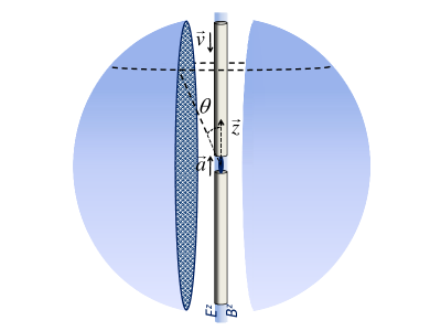
Figure 1: Electrons are injected with velocity $\vec{v}$ in a cylinder containing suitable electric, $E^{z}$, and magnetic, $B^{z}$, fields. Radiation is released near the center from an open window, which is surrounded by electromagnetic detectors lying on a sphere. This allows us to obtain the radiation spectral decomposition from which $dN_{k_{\bot}}^{{\rm M}}/dk_{\bot}$ is calculated.

The inertial-laboratory experiment: Let us set a pair of homogeneous and constant electric, $E^{z}=m_{q}\gamma a/q$, and magnetic, $B^{z}=-m_{q}\Omega\gamma/q$, fields defined by the free parameters (5) along the $z$ direction. Then, a charge $q$ is injected with transverse and longitudinal velocity components, $v_{\bot}$ and $v_{\parallel}$, respectively, in such a way that its 4-velocity $u^{\alpha}$ – satisfying the Lorentz law of force $m_{q}u^{\beta}\nabla_{\beta}u^{\alpha}=qF^{\alpha}_{\ \beta}u^{\beta}$ – is given by Eq. (3) Note_velocities . In the usual cylindrical coordinates, $(t,z,r,\phi)$ with the $z$ axis aligned with the 3-acceleration of the Rindler observers, the Minkowski line element is $ds^{2}=dt^{2}-dz^{2}-dr^{2}-r^{2}d\phi^{2}$, $u^{\alpha}=\gamma\left(\cosh(a\lambda),\sinh(a\lambda),0,\Omega\right)$, and

$$F_{\alpha\beta}=\begin{pmatrix}0&E^{z}&0&0\\ -E^{z}&0&0&0\\ 0&0&0&-rB^{z}\\ 0&0&rB^{z}&0\end{pmatrix}.$$ (13)

A prototype experimental apparatus is shown in Fig. 1, where a sub-picosecond charged bunch containing $\sim 10^{7}$ electrons W99 is injected in a cylinder containing $E^{z}$ and $B^{z}$. The radiation released near the center (where the charges are assumed to make the U turn) through an open window of length $L$ is collected by detectors set on a sphere with radius $R_{S}\gg L$. Since the charges emit radiation at typical wavelengths $\lambda\sim 1/a_{\rm tot}$, where $a_{\rm tot}=\gamma^{2}\sqrt{a^{2}+R^{2}\Omega^{4}}$ is the charge total proper acceleration, we should require $a_{\rm tot}\sim 1/\lambda\gg 1/L\approx 10^{17}~{}{\rm m/s^{2}}\times(1~{}{\rm m}/L)$ in order to avoid finite-size effects coming from the window. We note that magnetic and electric fields $B^{z}\approx 10^{-1}~{}{\rm T}$ and $E^{z}\approx 1~{}{\rm MV/m}$, respectively, achievable under present technology W08 , produce accelerations $a\sim 10^{17}~{}{\rm m/s^{2}}$ and $a_{\rm tot}\sim 10^{19}~{}{\rm m/s^{2}}$, where we have assumed $R\sim 10^{-1}~{}{\rm m}$. We also note that the radiation backreaction on the charge trajectory is negligible note7 .

The relevant quantity to be measured by the inertial experimentalists is the spectral-angular distribution

$$I(\omega,\theta,\phi)\equiv\frac{d{\cal E}(\omega,\theta,\phi)}{d\omega\,d(\cos\theta)\,d\phi}$$

of the emitted energy ${\cal E}$. From this and the one-photon relation ${\cal E}=\hbar\omega$, we get the corresponding photon number:

$$dN_{\omega\theta\phi}^{{\rm M}}={d\cal E}/{(\hbar\omega)}={I(\omega,\theta,\phi)}{(\hbar\omega)}^{-1}d\omega\,d(\cos\theta)\,d\phi,$$ (14)

which leads to the $k_{\bot}$-distribution of radiated photons

$$\frac{dN_{k_{\bot}}^{{\rm M}}}{dk_{\bot}}=\frac{k_{\bot}}{\hbar}\int_{0}^{2\pi}d\phi\int_{-\infty}^{\infty}\frac{dk_{z}}{(k_{\bot}^{2}+k_{z}^{2})^{3/2}}I(\omega,\theta,\phi)$$ (15)

(recall that $\omega^{2}=k_{\bot}^{2}+k_{z}^{2}$, $k_{\bot}=\omega\sin\theta$, and $d\omega\,d(\cos\theta)=\omega^{-2}k_{\bot}dk_{z}dk_{\bot}$). This is the quantity for which the uniformly accelerated observers can make a prediction, for, according to the Unruh effect UW84 , each emission of a Minkowski photon according to inertial observers corresponds to the absorption or emission of a Rindler photon from or to the Unruh thermal bath, respectively note3 . Therefore, the validity of the Unruh effect demands

$$\!\!\!\!\!\!\!\!\!\!\!\!\!\!\frac{dN_{k_{\bot}}^{{\rm M}}}{dk_{\bot}}\propto\left.\sum_{m=-\infty}^{\infty}\frac{d\Gamma_{k_{\bot}m}^{{\rm R}\,{\rm tot}}}{dk_{\bot}}\right|_{T=T_{\rm U}}$$

$$\!\!\!\!\!\!\!\!\!\!\!\!\!\!=\frac{q^{2}k_{\bot}}{\pi^{2}\hbar a}\sum_{m=-\infty}^{\infty}\Theta(m)\left[|K^{\prime}_{{im\Omega}/{a}}({k_{\bot}}/{a})|^{2}|J_{m}(k_{\bot}R)|^{2}\right.$$

$$\left.\!\!\!\!\!\!\!\!\!\!\!\!\!\!+(R\Omega)^{2}|K_{{im\Omega}/{a}}({k_{\bot}}/{a})|^{2}|J^{\prime}_{m}(k_{\bot}R)|^{2}\right]\cosh\left[\frac{\pi m\Omega}{a}\right]\!\!.$$ (16)

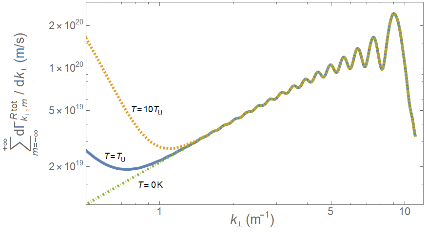
Figure 2: For the sake of illustration, we plot Eq. (12) summed in $m$ for different values of $T$ assuming $E^{z}=1$ MV/m, $B^{z}=10^{-1}$ T, $R=10^{-1}$ m, and injection energy $3.5$ MeV. The right-hand side of Eq. (16) corresponds to the solid-line curve.

The proportionality sign appears because the total number of photons depends on how long the experiment is run. In Fig. 2, we plot the right-hand side of Eq. (12) summed in $m$ for different values of $T$. The prediction given in Eq. (16) is represented by the solid-line curve ($T=T_{\rm U}$). We must keep in mind that due to finite-size effects coming from the window, greater experimental care must be taken in the region $k_{\bot}\lesssim 1/L$.

Virtual confirmation of the Unruh effect: Rather than waiting for experimentalists to confirm the prediction (16), here we perform a classical-electrodynamics calculation to prove it – to the extent one trusts classical electromagnetism. The spectral-angular distribution $I(\omega,\theta,\phi)$ is expressed in terms of the angular distribution of the radiated electric field $\vec{E}_{\rm rad}(t,\theta,\phi)$ Z12 :

$$I(\omega,\theta,\phi)=\frac{R_{S}^{2}}{\pi}\left|\int_{-\infty}^{\infty}dt\ \vec{E}_{rad}(t,\theta,\phi)e^{-i\omega t}\right|^{2}.$$ (17)

For our accelerated point-like charge, Eq. (17) can be written as (see, e.g., Ref. Z12 )

$$I(\omega,\theta,\phi)=\frac{q^{2}\omega^{2}}{4\pi^{2}}|\vec{F}(\omega,\theta,\phi)|^{2},$$ (18)

with

$$\vec{F}(\omega,\theta,\phi)=\hat{r}\times\int_{-\infty}^{\infty}d\lambda\frac{d\vec{r}_{q}}{d\lambda}f(\lambda),$$ (19)

where $\vec{r}_{q}(\lambda)=R\cos(\Omega\lambda)\hat{\rm i}+R\sin(\Omega\lambda)\hat{\rm j}+a^{-1}\cosh(a\lambda)\hat{\rm k}$ is the charge trajectory ($\{\hat{\rm i},\hat{\rm j},\hat{\rm k}\}$ being the usual Cartesian versors), $\hat{r}$ gives the observation direction, and $f(\lambda)\equiv\exp\left[-i\omega\left(\hat{r}\cdot\vec{r}_{q}(\lambda)-a^{-1}\sinh(a\lambda)\right)\right]$. The integrals in Eq. (19) can be solved by using

$$\int_{0}^{\infty}d\zeta\,\zeta^{-im\Omega/a+\alpha-1}\exp{[({i\omega/(2a)})\left(\Xi_{-}\zeta-\Xi_{+}/\zeta\right)]}$$

$$=2i^{\alpha}\exp\left[{\pi m\Omega}/{(2a)}\right]\left[\tan{(\theta}/{2})\right]^{-(im\Omega/a-\alpha)/2}$$

$$\times K_{im\Omega/a-\alpha}\left(\omega\sin\theta/a\right)$$ (20)

for $\alpha=0,\pm 1$ and $\Xi_{\pm}\equiv 1\pm\cos\theta$ note4 , combined with relations note5

$$\cos(\phi-\Omega\lambda)\exp{[-ik_{\bot}R\cos(\phi-\Omega\lambda)]}$$

$$=-\sum_{m}i^{m+1}J^{\prime}_{m}(-k_{\bot}R)\exp{[im(\phi-\Omega\lambda)]},$$ (21)

$$Rk_{\bot}\sin(\phi-\Omega\lambda)\exp{[-ik_{\bot}R\cos(\phi-\Omega\lambda)]}$$

$$=\sum_{m}mi^{m}J_{m}(-k_{\bot}R)\exp{[im(\phi-\Omega\lambda)]}.$$ (22)

Then, by using Eq. (18) into Eq. (14), we obtain

$$\!\!\!\!\!\!\!\!\frac{d^{2}N_{k_{\bot}k_{z}}^{{\rm M}}}{dk_{\bot}dk_{z}}=\frac{2q^{2}k_{\bot}}{\pi a^{2}\hbar\omega}\sum_{m=-\infty}^{\infty}\exp({{\pi m\Omega}/{a}})(|J_{m}(k_{\bot}R)|^{2}$$

$$\!\!\!\!\!\!\!\!\times|K^{\prime}_{{im\Omega}/{a}}\left({k_{\bot}}/{a}\right)|^{2}\!\!+\!(R\Omega)^{2}|J^{\prime}_{m}(k_{\bot}R)|^{2}|K_{{im\Omega}/{a}}\left({k_{\bot}}/{a}\right)|^{2}).$$

Finally, by integrating it in $k_{z}$ and performing the redefinition $k_{z}\to\kappa_{z}\equiv k_{z}/k_{\bot}$, we obtain

$$\frac{dN_{k_{\bot}}^{{\rm M}}}{dk_{\bot}}=\left(\frac{4\pi}{a}\int_{-\infty}^{\infty}\frac{d\kappa_{z}}{(1+\kappa_{z}^{2})^{1/2}}\right)\left.\sum_{m=-\infty}^{\infty}\frac{d\Gamma_{k_{\bot}m}^{{\rm R}\,{\rm tot}}}{dk_{\bot}}\right|_{T=T_{\rm U}}.$$ (23)

This concludes our proof of Eq. (16). The fact that the term between parentheses diverges is because the calculation above assumed a charge accelerating for infinite time, in which case an infinite number of photons is emitted for fixed $k_{\bot}$ element. In real experiments no divergence appears. We note that Eq.  (16) fits nicely real experiments with finite windows provided $a_{\rm tot}\gg 1/L$ note_SM .

Conclusions: We have proposed a simple experiment where the presence of the Unruh thermal bath is codified in the Larmor radiation emitted from an accelerated charge. Then, we carried out a straightforward classical-electrodynamics calculation to confirm it by ourselves. Unless one challenges classical electrodynamics, our results must be virtually considered as an observation of the Unruh effect.

SUPPLEMENTAL MATERIAL: Alternative derivation of Eq. (23) using standard quantum field theory

Here we provide an alternative derivation of Eq. (23) which reinforces that the infinite term between parenthesis appearing in this expression must be identified with the total Rindler proper time $\Delta\tau_{\rm R}$. In the inertial framework, the normalized physical modes of the electromagnetic field in polar coordinates [solutions of Eq. (6)] are

$$A_{\alpha}^{(I,m,k_{\bot},k_{z})} = k_{\bot}^{-1}\left(k_{z}g_{mk_{\bot}k_{z}},-\omega g_{mk_{\bot}k_{z}},0,0\right),$$

$$A_{\alpha}^{(II,m,k_{\bot},k_{z})} = k_{\bot}^{-1}\left(0,0,-mg_{mk_{\bot}k_{z}}/r,-ir\partial_{r}g_{mk_{\bot}k_{z}}\right),$$

where

$$g_{mk_{\bot}k_{z}}\equiv(8\pi^{2}\omega)^{-1/2}J_{m}\left(k_{\bot}r\right)e^{im\phi}e^{ik_{z}z}e^{-i\omega t},$$

$\epsilon=I,II$ labels the mode polarizations, $m\in\mathbb{Z}$, $k_{\bot}\in[0,+\infty)$, $k_{z}\in(-\infty,+\infty)$, and we recall that $\omega=\left(k_{\bot}^{2}+k_{z}^{2}\right)^{1/2}$. We expand $\hat{A}_{\alpha}$ in terms of inertial normal modes as

$$\hat{A}_{\alpha}=\sqrt{\hbar}\sum_{\epsilon,m}\int_{0}^{\infty}dk_{\perp}k_{\perp}\int_{-\infty}^{\infty}dk_{z}\left(\hat{a}_{(l)}A_{\alpha}^{(l)}+{\rm H.c.}\right)$$

with $(l)=(\epsilon,m,k_{\bot},k_{z})$. The $k_{\bot}$-distribution of Minkowski photons is given by

$$k_{\bot}^{-1}\frac{dN_{k_{\bot}}^{{\rm M}\,{\rm}}}{dk_{\bot}}=\sum_{\epsilon,m}\int_{-\infty}^{\infty}dk_{z}\ |{\cal A}^{{\rm M}\,{\rm em}}_{(l)}|^{2},$$ (24)

where

$$|{\cal A}^{{\rm M}\,{\rm em}}_{(l)}|=\hbar^{-1}\left|\int d^{4}x\sqrt{-g}j^{\alpha}\,\langle l|\hat{A}_{\alpha}|0\rangle_{M}\right|$$

and we recall that $j^{\alpha}$ is given by Eq. (4). We note that Eq. (24) [in contrast to Eqs. (10) and (11)] does not carry any thermal factor because the Minkowski vacuum, $|0\rangle_{M}$, is a no-particle state according to inertial observers. The photon emission amplitudes for both polarizations can be written as

$${\cal A}^{{\rm M}\,{\rm em}}_{(I,m,k_{\bot},k_{z})} = \hbar^{-1}\langle I,m,k_{\bot},k_{z}|iS_{I}|0\rangle_{M}$$ (25)

$$= \frac{iqJ_{m}\left(k_{\bot}R\right)}{2\pi k_{\bot}\sqrt{2\hbar\omega}}\int_{-\infty}^{\infty}d\lambda\ h(\lambda)$$

$$\times \left[k_{z}\cosh{(a\lambda)}-\omega\sinh{(a\lambda)}\right],$$

$${\cal A}^{{\rm M}\,{\rm em}}_{(II,m,k_{\bot},k_{z})} = \hbar^{-1}\langle II,m,k_{\bot},k_{z}|iS_{I}|0\rangle_{M}$$ (26)

$$= \frac{qR\Omega J^{\prime}_{m}(k_{\bot}R)}{2\pi\sqrt{2\hbar\omega}}\int_{-\infty}^{\infty}d\lambda\ h(\lambda),$$

where

$$h(\lambda)=\exp{\left(-im\Omega\lambda-\frac{i}{a}\left[k_{z}\cosh{(a\lambda)}-\omega\sinh{(a\lambda)}\right]\right)}$$

and $\lambda$ is related to the inertial time by $t=a^{-1}\sinh{(a\lambda)}$, i.e., $\lambda$ is the proper time of the Rindler observer at $\xi=0$. This variable change is a necessary maneuver to allow us to express the emitted photon number in terms of $\Delta\tau_{\rm R}$.

In order to obtain the total emitted photon number per fixed $k_{\bot}$, we must square the absolute values of the amplitudes (25) and (26) and insert them in Eq. (24). From this procedure, we end up with an integral $\int_{-\infty}^{\infty}d\lambda\int_{-\infty}^{\infty}d\lambda^{\prime}\ (\cdots)$ which can be expressed as $\int_{-\infty}^{\infty}d\tau_{\rm R}\int_{-\infty}^{\infty}d\sigma\ (\cdots)$ once we write $\tau_{\rm R}=(\lambda+\lambda^{\prime})/2$ and $\sigma=\lambda-\lambda^{\prime}$. As a result, we obtain for the emitted photon number

$$k_{\bot}^{-1}\frac{dN_{k_{\bot}}^{{\rm M}\,{\rm}}}{dk_{\bot}}=\Delta\tau_{\rm R}\sum_{m}\frac{q^{2}}{8\pi^{2}\hbar}\int_{-\infty}^{\infty}d\sigma\int_{-\infty}^{\infty}dk_{z}$$

$$\times\left[\left({\cal N}_{I}+{\cal N}_{II}\right)\exp[-im\Omega\sigma-2ia^{-1}\omega\sinh{\left(a\sigma/2\right)}]\right],$$

with

$$\Delta\tau_{\rm R} = \int_{-\infty}^{\infty}d\tau_{\rm R},$$

$${\cal N}_{I} = \frac{|J_{m}(k_{\bot}R)|^{2}}{\omega}\left[\left(\frac{\omega}{k_{\bot}}\right)^{2}-\cosh^{2}\left({\frac{a\sigma}{2}}\right)\right],$$

$${\cal N}_{II} = \frac{|J^{\prime}_{m}(k_{\bot}R)|^{2}}{\omega}(R\Omega)^{2},$$

where we have made the transformation $(k_{z},\omega)\to(\tilde{k}_{z},\tilde{\omega})$ with

$$\tilde{k}_{z} \equiv k_{z}\cosh(a\tau_{\rm R})-\omega\sinh(a\tau_{\rm R}),$$

$$\tilde{\omega} \equiv \omega\cosh(a\tau_{\rm R})-k_{z}\sinh(a\tau_{\rm R}),$$

and dropped the tildes, eventually. After solving the remaining integrals in $\sigma$ and $k_{z}$, we obtain

$$\frac{dN_{k_{\bot}}^{{\rm M}}}{dk_{\bot}}=\Delta\tau_{\rm R}\frac{q^{2}k_{\bot}}{\pi^{2}\hbar a}\sum_{m}\Theta(m)\left[|K^{\prime}_{{im\Omega}/{a}}({k_{\bot}}/{a})|^{2}\right.$$

$$\left.\times|J_{m}(k_{\bot}R)|^{2}+(R\Omega)^{2}|K_{{im\Omega}/{a}}({k_{\bot}}/{a})|^{2}|J^{\prime}_{m}(k_{\bot}R)|^{2}\right]$$

$$\times\cosh\left[\frac{\pi m\Omega}{a}\right],$$ (27)

which coincides with Eq. (23) provided we make the identification

$$\Delta\tau_{\rm R}\leftrightarrow\left(\frac{4\pi}{a}\int_{-\infty}^{\infty}\frac{d\kappa_{z}}{\left(1+\kappa_{z}^{2}\right)^{1/2}}\right).$$

References

• (1) W. G. Unruh, “Notes on black hole evaporation,” Phys. Rev. D 14, 870 (1976).
• (2) Actually, the Unruh effect was communicated one year earlier in the $1^{\rm st}$ Marcel Grossmann meeting at Trieste but the corresponding proceedings only appeared in 1977 U77 .
• (3) W. G. Unruh, “Particle detector and black holes,” in Proceedings of the $1^{st}$ Marcel Grossmann meeting on General Relativity, (North-Holland Publishing Company, Amsterdam, 1977).
• (4) S. A. Fulling, “Nonuniqueness canonical field quantization in Riemaninan space-time,” Phys. Rev. D 7, 2850 (1973).
• (5) P. C. W. Davies, “Scalar particle production in Schwarzschild and Rindler metrics,” J. Phys. A: Gen. Phys. 8, 609 (1975).
• (6) J. J. Bisognano and E. H. Wichmann, “On the duality condition for quantum fields,” J. Math. Phys. 17, 303 (1976).
• (7) G. L. Sewell, “Quantum fields on manifolds: PCT and gravitationally induced thermal states,” Ann. Phys. 141, 201 (1982).
• (8) W. Unruh and R. M. Wald, “What happens when an accelerating observer detects a Rindler particle,” Phys. Rev. D 29, 1047 (1984).
• (9) L. C. B. Crispino, A. Higuchi, and G. E. A. Matsas, “The Unruh effect and its applications,” Rev. Mod. Phys. 80, 787 (2008).
• (10) S. A. Fulling and G. E. A. Matsas, “Unruh effect,” Scholarpedia, 9(10):31789 (2014).
• (11) J. S. Bell and J. M. Leinaas, “Electrons as accelerated thermometers,” Nucl. Phys. B 212, 131 (1983).
• (12) R. Müller, “Decay of accelerated particles,” Phys. Rev. D 56, 953 (1997).
• (13) D. A. T. Vanzella and G. E. A. Matsas, “Decay of accelerated protons and the existence of the Fulling-Davies-Unruh effect,” Phys. Rev. Lett. 87, 151301 (2001).
• (14) H. Suzuki and K. Yamada, “Analytic evaluation of the decay rate for an accelerated proton,” Phys. Rev. D 67, 065002 (2003).
• (15) D. A. T. Vanzella and G. E. A. Matsas “Weak decay of uniformly accelerated protons and related processes,” Phys. Rev. D 63, 014010 (2001).
• (16) P. Chen and T. Tajima, “Testing Unruh Radiation with Ultraintense Lasers,” Phys. Rev. Lett. 83, 256 (1999).
• (17) N. Oshita, K. Yamamoto, and S. Zhang, “Quantum radiation produced by a uniformly accelerating charged particle in thermal random motion,” Phys. Rev. D 93, 085016 (2016).
• (18) R. Schutzhold, G. Schaller, and D. Habs, “Signatures of the Unruh effect from electrons accelerated by ultrastrong laser fields,” Phys. Rev. Lett. 97, 121302 (2006).
• (19) A. Higuchi, G. E. A. Matsas, and D. Sudarsky, “Bremsstrahlung and zero-energy Rindler photons,” Phys. Rev. D 45, R3308 (1992).
• (20) A. Higuchi and G. E. A. Matsas, “Fulling-Davies-Unruh effect in classical field theory,” Phys. Rev. D 48, 689 (1993).
• (21) S. Cruz y Cruz and B. Mielnik, “Non-inertial quantization: Truth or illusion,” Journal of Physics: Conference Series 698, 012002 (2016).
• (22) Setting $Z\equiv z-a^{-1}=0$ at the point where the charge makes the “U turn” in the longitudinal direction ($z$) and adopting orientation such that $E^{z}<0$, the injection velocity components are given by $v_{\bot}=\Omega R/(1+aZ_{i})$ and $v_{\parallel}=-\sqrt{a^{2}Z_{i}^{2}+2aZ_{i}}/(1+aZ_{i})$, where $Z_{i}>0$ is the position where the injection occurs.
• (23) X. J. Wang, Producing and measuring small electron bunches in Proceedings of the 1999 particle accelerator conference (IEEE, N.Y., 1999).
• (24) For wavelengths $\lambda$ larger than the bunch size, interference plays an important role and the whole set of charges acts collectively as a single one with magnitude $q$ equal to the sum of all charges. This magnifies the emitted power which scales as $q^{2}$.
• (25) T. P. Wangler, RF Linear Accelerators, 2nd edition (Wiley-VCH, Weinheim, 2008).
• (26) Using Larmor formula, we see that for these parameters, the charged bunch will emit $\sim 10\times L/(1~{}{\rm m})~{}{\rm GeV}$, which is small even when compared to the fraction of the total kinetic energy carried in the form of rotational energy of the bunch, $\sim 10^{4}~{}{\rm GeV}$.
• (27) A. Zangwill, Modern Electrodynamics (Cambridge University Press, Cambridge, 2012).
• (28) We note, in addition, that due to angular momentum conservation, the absorption of a photon with $m>0$ by the charge as seen by accelerated observers corresponds to the emission of a photon with $m<0$ according to inertial ones.
• (29) This expression can be obtained from Eq. 8.432.7 of Ref. GR after the substitution $e^{a\lambda}\to\zeta$ and “rotation” to the positive imaginary axis.
• (30) I. S. Gradshteyn and I. M. Ryzhik, Table of Integrals, Series and Products (Academic Press, New York, 1980).
• (31) These identities are obtained by properly differentiating Eq. 8.511.4 of Ref. GR (after the substitution $z\to-\omega R\sin\theta$ and $\varphi\to\phi-\Omega\lambda$).
• (32) See Supplemental Material below for an alternative derivation of Eq. (23), which allows us to identify the term between parentheses with $\Delta\tau_{R}$ and clarify the proportionality sign in Eq. (16).