B fields in OB stars (BOB): The magnetic triple stellar system HD 164492C in the Trifid nebula.

Abstract

HD 164492C is a spectroscopic triple stellar system that has been recently detected to possess a strong magnetic field. We have obtained high-resolution spectroscopic and spectropolarimetric observations over a timespan of two years and derived physical, chemical, and magnetic properties for this object. The system is formed by an eccentric close spectroscopic binary (Ca1-Ca2) with a period of 12.5 days, and a massive tertiary Cb. We calculated the orbital parameters of the close pair, reconstructed the spectra of the three components, and determined atmospheric parameters and chemical abundances by spectral synthesis. From spectropolarimetric observations, multi-epoch measurements of the longitudinal magnetic fields were obtained. The magnetic field is strongly variable on timescales of a few days, with a most probable period in the range of 1.4–1.6 days. Star Cb with $T_{\mathrm{eff}}$ $\sim$ 25 000 K is the apparently fastest rotator and the most massive star of this triple system and has anomalous chemical abundances with a marked overabundance of helium, 0.35$\pm$0.04 by number. We identified this star as being responsible for the observed magnetic field, although the presence of magnetic fields in the components of the Ca pair cannot be excluded. Star Ca1 with a temperature of about 24 000 K presents a normal chemical pattern, while the least massive star Ca2 is a mid-B type star ($T_{\mathrm{eff}}$ $\sim$ 15 000 K) with an overabundance of silicon. The obtained stellar parameters of the system components suggest a distance of 1.5 kpc and an age of 10–15 Myr.

1 Introduction

The multiple star HD 164492 (=ADS 10991) is a trapezium-like stellar system belonging to the Trifid Nebula, an active star forming region. The nebula is ionised by the O7.5 Vz (Sota et al., 2014) star HD 164492A, which is the central object of this multiple. The central part of the system is formed by five bright ($V=7.4-12.2$ mag) visual components in a non-hierarchical configuration (A to E; Kohoutek et al., 1999). The relevance of studying this multiple has increased following the recent discovery of a magnetic field of about 500 G in one of its components, the subsystem HD 164492C (Hubrig et al., 2014), by the BOB (“B fields in OB stars”) collaboration (Morel et al., 2014, 2015). In addition, Hubrig et al. (2014) reported that HD 164492C is an early-B type double-lined spectroscopic binary, and possibly a triple. No quantitative analyses of the components of HD 164492C is available in the literature so far.

The main goal of the present work is to describe the physical and chemical properties of this interesting system as completely as possible, in particular its magnetic field, in order to contribute to the understanding of the conditions under which magnetic fields are developed in massive stars. Only a small fraction of stars (5–7%) with radiative envelopes possess strong large-scale organised magnetic fields (Grunhut & Wade, 2013; Morel et al., 2015), which can be generated during the star formation process (fossil fields, e.g. Borra et al., 1982; Moss, 2001), or dynamo action taking place in the rotating stellar cores, or they could be products of a merger process. While the first two scenarios are unable to explain a number of observational phenomena (e.g. Ferrario et al., 2015), the magnetic fields could form when two proto-stellar objects merge late on their approach to the main sequence and when at least one of them has already acquired a radiative envelope (Ferrario et al., 2009). The origin of magnetic fields in massive stars is still a major unresolved problem in astrophysics.

Sections 2 to 4 describe the observations, the reconstruction of the spectra of the stellar components, and the orbital analysis of the close binary subsystem. The physical parameters and chemical abundances are derived in Sect. 5 and 6, while the magnetic field is discussed in Sect. 8. The main results are summarised in Sect. 9.

2 Spectroscopic and spectropolarimetric observations

We have obtained high-resolution spectroscopic and spectropolarimetric observations over a timespan of two years with the ESO spectrographs UVES, FEROS, and HARPS. The FEROS echelle spectrograph on the 2.2-m telescope at La Silla produces spectra with a resolving power of 48 000 and a wavelength coverage from 3500 to 9200 Å. Our UVES observations cover two spectral regions: the blue spectrum between 3300 and 4530 Å with a resolving power of $R=80\,000$ and the red spectrum covering the range from 5700 to 9450 Å with $R=110\,000$. The polarimetric spectra of HARPS have a resolving power of $R=115\,000$ and cover the spectral range from 3780 to 6910 Å, with a gap between 5259 and 5337 Å. The four FEROS spectra were taken in August 2013, while the 15 UVES spectra were taken between April and August 2014. The typical signal-to-noise ratio at $\lambda=4200$ Å is 280 for the UVES spectra and 110 for the FEROS spectra. With HARPS we acquired 11 spectropolarimetric observations in 5 observing runs in June 2013, April 2014, March 2015, June 2015, and October 2015. The signal-to-noise ratio in the Stokes $I$ spectra is about 300 per pixel above 4600 Å, decreasing in the blue to about 150 at 4000 Å.

The basic data reduction and calibration was performed using specific ESO reduction pipelines. UVES spectra were re-reduced using standard tasks of the NOAO/IRAF package.

In the red spectral region, the spectra required some processing to remove features not belonging to the stars: telluric and interstellar absorption lines, and, in the case of the HARPS spectra, nebular emission lines. Emission features appear with different intensity in spectra taken with the fibre-fed spectrograph HARPS, while they are absent in observations taken with the slit spectrograph UVES. The fact that these emissions are removed through background subtraction during the reduction process of UVES data, indicates that the origin of these emissions is not circumstellar but nebular, since any circumstellar structure would have been included in the object extraction aperture. We obtained an emission line master spectrum by averaging background-aperture spectra of several UVES observations. This emission line spectrum was scaled to mimic the intensity of emission lines in each HARPS spectrum and then subtracted.

During this process we identified and measured all relevant nebular lines. The line identification was done using the lists by Stasińska (2009). The average radial velocity of nebular lines is $-4.8\pm 1.8$ km s^-1. Most emission lines do not overlap crucial stellar lines, but the detection and removal of small He i emissions was particularly important to avoid the distortion of stellar He i line profiles.

3 Separation of spectral components

Line profiles of HD 164492C show clear variations on time-scales of a few days. The majority of the line profiles presents a complex structure suggesting the existence of more than two spectroscopic components. We propose as the most simple interpretation, the presence of a fixed broad-line spectrum superimposed with a double-lined spectroscopic binary. The results of the spectral disentangling performed under this hypothesis and the modelling of composite spectra with spectral synthesis confirmed that this system is indeed a hierarchical triple. The presence of a third source is also supported by the fact that HD 164492C is a visual binary with a separation of 0.08″(González & Veramendi, 2016; Yusef-Zadeh et al., 2005). This visual pair can be confidently considered as physically bound, since the probability of chance alignment for two stars of magnitude $V$=9.0–9.5 mag ($J$=8.6–9.2 mag) is very low. From the two-dimensional star density, derived using the 2MASS Catalogue, we estimated that the probability of having a companion brighter than $J$=10 mag at an angular distance smaller than 0.08″is about 1:$1.3\times 10^{6}$. Following the conventional nomenclature of multiple stars, we named the companions of the close binary as HD 164492Ca1 and HD 164492Ca2, and the more distant star with the broad-line spectrum as HD 164492Cb.

We separated the three spectral components applying the method of González & Levato (2006), and assuming that the third star (Cb) has constant radial velocity. Considering the different wavelength coverage of the HARPS and UVES spectra, we performed the calculations separately in three spectral regions: 3700–4530 Å (UVES+HARPS), 3800–5250 Å (HARPS), and 5680–6800 Å (UVES+HARPS). From the composite spectra we made a first estimation of the spectral types (B1 for components Ca1 and Cb, and B4-B6 for Ca2) and according to this we selected spectra of reference stars as a starting point for the iterative disentangling process. We used high-resolution archival spectra of slowly-rotating stars HR 2222 (B1 V) for Ca1 and Cb and HR 1288 (B4 V) for Ca2. These spectra have been taken with the UVES and FEROS spectrographs as part of other observing programmes. The reference spectra were scaled and convolved with theoretical rotational profiles to mimic the lines of the components of HD 164492C.

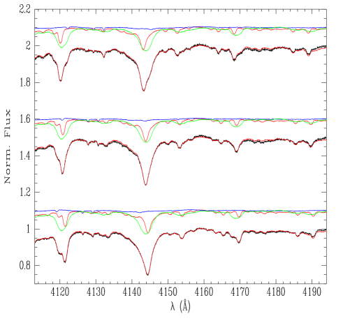
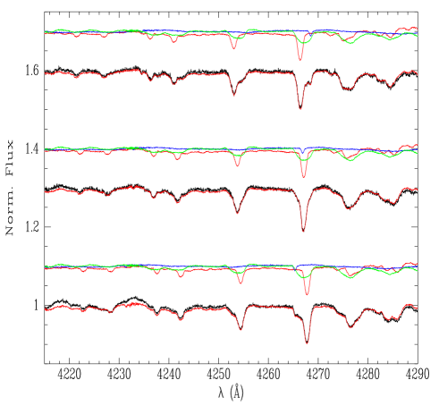
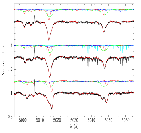
Figure 1: Selected regions in the UVES spectra showing the separation of the spectral components at three different phases. The two upper panels correspond to UVES spectra with orbital phases 0.14, 0.35, and 0.81 (from bottom to top) and the lower panel to HARPS spectra with phases 0.02, 0.33, and 0.56. For each phase we show in the upper part the reconstructed spectra of the components Cb (green), Ca1 (red), and Ca2 (blue), and below the observed spectrum (small black dots) overplotted with the sum of the three reconstructed spectra (red line). In the lower panel modelled telluric lines are shown in light blue. The nebular $[$O iii$]$ emission line is visible at 5007 Å.

To recover the intrinsic intensities of the spectra of the individual components, it is necessary to scale the separated spectra according to the flux contribution of each star. To this aim, we derived from the spectral types a first estimate of $T_{\mathrm{eff}}$ and $\log g$. Then we estimated the flux contribution of each component as a function of wavelength using synthetic spectra from the grid calculated by Lanz & Hubeny (2007) and the stellar radii estimated from the Geneva stellar models (Ekström et al., 2012) assuming that all three stars have the same age and requiring the masses of stars Ca1 and Ca2 to be consistent with the spectroscopic mass ratio. In a later stage, the relative flux of the components was recalculated using synthetic spectra with the appropriate atmospheric parameters and chemical abundances (see Sect. 5).

The noise level of the separated spectra is about 1/1300 of the original continuum at $\lambda$ 4200 Å in the first spectral region, about 1/650 at 5000 Å, and 1/800 in the red region. The final signal-to-noise of the reconstructed spectra depends also on the relative flux contribution of each star, which are approximately 0.55–0.60 for Cb, 0.35–0.40 for Ca1, and 0.05–0.07 for Ca2 (see Sect. 5). Thus, after scaling, the separated spectra have a signal-to-noise ratio of the order of 500 for the most massive stars and of only 50 for the star Ca2.

Table 1: Radial velocities of the spectroscopic binary HD 164492Ca. Column 1: Heliocentric Julian date; Column 2: orbital phase calculated with respect to the periastron passage $T_{\pi}$ (see Table 2); Column 3 and 5: radial velocities for stars Ca1 and Ca2; Columns 4 and 6: residuals observed-minus-calculated; Column 7: Spectrograph.

HJD	$\phi$	RVCa1		(O-C)1	RVCa2		(O-C)2	Instrument
		km s-1		km s-1	km s-1		km s-1
2 456 445.7946	0.5559	$-$28.4 $\pm$	1.0	1.7	44.1 $\pm$	0.6	0.0	HARPS
2 456 446.7934	0.6355	$-$36.6 $\pm$	0.9	2.0	62.3 $\pm$	0.7	$-$0.9	HARPS
2 456 522.6844	0.6898	$-$42.7 $\pm$	1.4	1.2	75.0 $\pm$	1.9	0.0	FEROS
2 456 523.7039	0.7711	$-$49.9 $\pm$	1.2	0.4	88.9 $\pm$	1.9	$-$0.7	FEROS
2 456 524.6224	0.8444	$-$52.9 $\pm$	1.6	$-$0.5	98.8 $\pm$	2.6	4.5	FEROS
2 456 525.6624	0.9273	$-$32.3 $\pm$	1.4	2.6	59.1 $\pm$	2.0	4.3	FEROS
2 456 770.7700	0.4808	$-$22.5 $\pm$	1.0	$-$1.2	24.0 $\pm$	0.9	$-$0.2	HARPS
2 456 771.7850	0.5618	$-$28.3 $\pm$	0.9	2.5	46.3 $\pm$	0.9	0.7	HARPS
2 456 772.7707	0.6404	$-$39.4 $\pm$	0.8	$-$0.2	63.1 $\pm$	0.8	$-$1.2	UVES
2 456 777.8085	0.0423	73.9 $\pm$	0.9	$-$1.2	$-$192.7 $\pm$	0.7	0.2	UVES
2 456 779.8951	0.2088	25.4 $\pm$	1.0	$-$0.3	$-$83.5 $\pm$	0.9	$-$2.0	UVES
2 456 786.8817	0.7661	$-$51.2 $\pm$	0.8	$-$1.2	88.2 $\pm$	0.5	$-$0.6	UVES
2 456 837.6044	0.8125	$-$53.4 $\pm$	0.8	$-$1.2	94.3 $\pm$	0.5	0.3	UVES
2 456 869.5077	0.3576	$-$4.2 $\pm$	0.9	$-$0.1	$-$12.7 $\pm$	0.5	1.9	UVES
2 456 879.6971	0.1705	36.1 $\pm$	0.9	$-$0.2	$-$105.2 $\pm$	0.7	0.4	UVES
2 456 883.4874	0.4729	$-$22.5 $\pm$	0.9	$-$2.2	20.7 $\pm$	0.4	$-$1.2	UVES
2 456 887.4936	0.7925	$-$52.4 $\pm$	0.9	$-$0.9	93.3 $\pm$	0.5	1.1	UVES
2 456 894.6261	0.3614	$-$3.8 $\pm$	0.9	0.9	$-$12.3 $\pm$	0.6	0.9	UVES
2 456 898.5681	0.6759	$-$43.8 $\pm$	0.9	$-$1.2	71.8 $\pm$	0.7	$-$0.3	UVES
2 456 919.5607	0.3506	$-$3.1 $\pm$	1.0	$-$0.2	$-$17.0 $\pm$	0.5	0.1	UVES
2 456 923.5111	0.6658	$-$41.7 $\pm$	0.9	$-$0.1	67.9 $\pm$	1.0	$-$2.0	UVES
2 456 926.5385	0.9073	$-$42.8 $\pm$	0.8	0.7	72.2 $\pm$	0.7	$-$2.0	UVES
2 456 929.4996	0.1435	43.8 $\pm$	0.8	$-$1.2	$-$126.4 $\pm$	0.9	$-$1.4	UVES
2 457 091.8426	0.0944	59.1 $\pm$	1.3	$-$3.6	$-$163.8 $\pm$	1.0	1.3	HARPS
2 457 092.8282	0.1730	35.9 $\pm$	0.9	0.4	$-$103.4 $\pm$	0.6	0.5	HARPS
2 457 093.8478	0.2544	17.2 $\pm$	0.7	2.3	$-$57.5 $\pm$	0.6	$-$0.1	HARPS
2 457 094.8153	0.3316	3.2 $\pm$	0.7	3.0	$-$24.0 $\pm$	0.7	0.3	HARPS
2 457 178.6948	0.0231	69.5 $\pm$	1.4	0.6	$-$180.9 $\pm$	1.1	$-$2.0	HARPS
2 457 179.7426	0.1067	60.2 $\pm$	1.4	2.0	$-$156.5 $\pm$	0.9	$-$1.8	HARPS
2 457 317.5185	0.0977	64.6 $\pm$	2.0	3.1	$-$163.9 $\pm$	2.0	$-$1.7	HARPS

As illustration, Figure 1 shows for three different orbital phases how the reconstructed spectra combine to reproduce the observed profiles. For the star Ca2, lines of Si ii ($\lambda\lambda$ 4128, 4130, 5041, 5056), Fe ii ($\lambda\lambda$ 4233, 5018), C ii ($\lambda$ 4267), and He i ($\lambda\lambda$ 4121, 4144, 5015, 5047) can be distinguished. For the most massive stars, besides the mentioned lines of C ii and He i, the most noticeable lines in the plot correspond to Al iii ($\lambda$ 4150), Fe iii ($\lambda$ 4165), and O ii ($\lambda\lambda$ 4133, 4153, 4169, 4185, 4190). A complete spectral atlas of the component spectra with the line identification is included in the Appendix (available online). We conclude that the three mentioned spectral components represent satisfactorily the observed spectral content and variations.

The reconstructed spectrum of Ca1, the primary companion of the close binary, shows a morphology typical of a B1 V star, with lines of He i, C ii, N ii, O ii, Al iii, Si iii-iv, S ii-iii, and Fe iii. The spectrum of Cb seems to be very similar to Ca1, but with broader metal lines because of a higher rotational velocity. Remarkable are the unusually strong He i lines, indicating a He-rich nature for this star. The faint star Ca2 is a mid-B type star: only a few strong lines of He i, C ii, Mg ii, Si ii, S ii and Fe ii can be identified in its spectrum (see Appendix).

4 Orbital elements

Radial velocities of the close binary Ca were measured by cross-correlations during the spectral separation process. FEROS spectra, which were not considered in the reconstruction of component spectra because of their lower resolution, were included in the radial velocity measurements. We used as templates the observed spectra of reference stars mentioned in the previous section: HR 2222 for Ca1 and HR 1288 for Ca2. Before carrying out the cross-correlations, radial velocities of template spectra were corrected by measuring several tens of metallic spectral lines. Table 1 lists the measured radial velocities. Orbital phase zero corresponds to the periastron passage.

During the spectral disentangling only one fixed value for the radial velocity of star Cb was fitted. Afterwards, to look for possible variations in the spectrum of this star, we removed the spectra of Ca1 and Ca2 from the observed spectra using the reconstructed spectra of these components, and measured the resulting spectra, which would be individual spectra of star Cb. The velocity of this star is constant within uncertainties, with a mean value of $-6.3$ km s^-1 and a standard deviation of 2.8 km s^-1, which is lower than the typical measurement errors. The mean radial velocity of Cb agrees with the barycentric velocity of the binary Ca and that of the Trifid nebula ($-4.8\pm 1.8$ km s^-1, see Sect. 2).

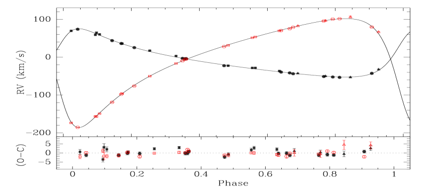
Figure 2: Radial velocity curves of HD 164492Ca. The bottom panel shows residuals (observed-minus-calculated). Filled (open) symbols correspond to the primary (secondary) star, circles indicate measurements with UVES, squares with HARPS, and triangles with FEROS.

Table 2: Orbital parameters of the binary HD 164492Ca.

Parameter	Units	Value
$P$	d	12.5349 $\pm$	0.0008
$T_{\mathrm{I}}$	d	2 456 692.94 $\pm$	0.03
$T_{\pi}$	d	2 456 689.54 $\pm$	0.03
$K_{\mathrm{1}}$	km s-1	63.8 $\pm$	0.8
$K_{\mathrm{2}}$	km s-1	143.8 $\pm$	0.7
$\omega$	rad	5.29 $\pm$	0.01
$e$		0.532 $\pm$	0.004
$q$		0.444 $\pm$	0.006
$a_{\mathrm{1}}\sin i$	$R_{\odot}$	13.4 $\pm$	0.2
$a_{\mathrm{2}}\sin i$	$R_{\odot}$	30.2 $\pm$	0.2
$a\sin i$	$R_{\odot}$	43.5 $\pm$	0.2
$M_{\mathrm{1}}\sin^{3}i$	$M_{\odot}$	4.89 $\pm$	0.06
$M_{\mathrm{2}}\sin^{3}i$	$M_{\odot}$	2.17 $\pm$	0.04
$\gamma$	km s-1	$-$7.3 $\pm$	0.3
$n$		30
$\sigma_{\mathrm{1}}$	km s-1	1.65
$\sigma_{\mathrm{2}}$	km s-1	1.61

A Keplerian orbit was fitted to the observed radial velocities by least squares. Figure 2 shows the radial velocity curves and Table 2 lists the fitted orbital parameters: period $P$, time of periastron passage $T_{\pi}$, radial velocity amplitudes $K_{\mathrm{1}}$ and $K_{\mathrm{2}}$, centre-of-mass velocity $\gamma$, argument of periastron $\omega$, and eccentricity $e$. We list also the following derived parameters: time of primary conjunction $T_{\mathrm{I}}$, projected orbital semiaxis $a\sin i$, and minimum masses $M\sin^{3}i$. The last three rows are the number of observations and the global RMS of the residuals for the primary ($\sigma_{\mathrm{1}}$) and the secondary ($\sigma_{\mathrm{2}}$). In fact, standard deviations differ for the three instruments, being about 1.1 km s^-1 for UVES, 1.7 km s^-1 for HARPS, and 2.5 km s^-1 for FEROS. These values are somewhat larger than the formal measurement errors, and are probably a better estimate of the actual velocity uncertainties.

5 Spectral analysis

The determination of physical and chemical properties of stellar atmospheres through spectral analysis and modelling is more complicated in the case of spectroscopic multiple systems, because more parameters need to be accounted for. A comprehensive solution requires the physical model of the system to match the observed composite and disentangled spectra and to provide consistent ages, spectroscopic distances, the mass ratio for Ca2/Ca1 (from the orbital solution) and flux scaling factors for the components simultaneously. Observationally, this is complicated by the fact that low-frequency modulations are not recovered by disentangling techniques based on relative Doppler shifts. For that reason broad features like hydrogen lines and broad He lines, whose profiles are significantly wider than the shifts due to the orbital motion, cannot be fitted individually for each component. Moreover, relative fluxes are in principle unknown. Unless they are adopted from a different information source – as e.g. in detached eclipsing binaries –, they are additional parameters, however mutually dependent on stellar effective temperatures and radii. These facts make the spectral analysis of the various stellar components to be interdependent.

Table 3: Model atoms for non-LTE calculations. Updated models as described by Nieva & Przybilla (2012) are marked with *.

Ion	Model atom
H i	Przybilla & Butler (2004)
He i/ii	Przybilla (2005)
C ii/iii	Nieva & Przybilla (2006, 2008)
N ii	Przybilla & Butler (2001)*
O i/ii	Przybilla et al. (2000), Becker & Butler (1988)*
Ne i	Morel & Butler (2008)*
Mg ii	Przybilla et al. (2001)
Al iii	Przybilla (in prep.)
Si ii-iv	Przybilla & Butler (in prep.)
S ii/iii	Vrancken et al. (1996)*
Fe ii/iii	Becker (1998), Morel et al. (2006)*

We used a hybrid non-LTE approach for the quantitative analysis of the composite and separated spectra, in analogy to the methods described by Nieva & Przybilla (2007, 2012) and Przybilla et al. (2016) for the study of single (He-strong) B-type stars, extending them here where necessary for the multiple star case. In brief, this approach is based on plane-parallel, hydrostatic, chemically homogeneous and line-blanketed model atmospheres that were computed with the code Atlas9 (Kurucz, 1993) under the assumption of radiative and local thermodynamic equilibrium (LTE). For the parameter range studied here, these are equivalent to hydrodynamic or hydrostatic line-blanketed non-LTE model atmospheres within the line-formation regions (Nieva & Simón-Díaz, 2011; Nieva & Przybilla, 2007; Przybilla et al., 2011). Non-LTE level populations and synthetic spectra were calculated with recent versions of the codes Detail and Surface (Giddings, 1981; Butler & Giddings, 1985, both updated by one of us (KB)), employing comprehensive model atoms as summarised in Table 3.

Table 4: Atmospheric and fundamental stellar parameters and chemical abundances ( $\log X/\mathrm{H}+12$) for the three components of HD 164492C. Uncertainties are $\sim$0.2 dex for abundances. Standard values (CAS) were taken from Nieva & Przybilla (2012), except those marked with asterisks, which are preliminary values from Przybilla et al. (2013). Uncertainties for the CAS values are standard deviations.

Parameter	HD 164492Cb	HD 164492Ca1	HD 164492Ca2	CAS
Spectral Type	B1 V/IV He-strong	B1 V	B4-6 V
$T_{\mathrm{eff}}$ (K)	$25\,000\pm 500$	$24\,000\pm 500$	$15\,000\pm 1000$
$\log g$ (cgs)	$3.90\pm 0.15$	$4.00\pm$ 0.20	4.30a
$\xi$ (km s-1)	$2\pm 1$	$2\pm 1$	$2\pm 1$
$v\sin i$ (km s${}^{-1})$	$135\pm 5$	$48\pm 5$	$19\pm 2$
$\zeta$ (km s-1)	…	$25\pm 5$	$12\pm 2$
$y$ (number fraction)	$0.35\pm 0.04$	$0.089\pm 0.010$	$0.089\pm 0.010$	$0.089\pm 0.002$
C ii/iii	8.13	8.50	…	$8.33\pm 0.04$
N ii	7.78	7.93	…	$7.79\pm 0.04$
O i/ii	9.16	8.91	…	$8.76\pm 0.05$
Ne i	7.59	8.15	…	$8.09\pm 0.05$
Mg ii	7.36	7.62	…	$7.56\pm 0.05$
Al iii	6.23	6.49	…	*$6.30\pm 0.07$
Si ii-iv	7.81	7.59	…	$7.50\pm 0.05$
S ii	7.15	7.21	…	*$7.14\pm 0.06$
Fe iii	7.52	7.61	…	$7.52\pm 0.03$
$M/M_{\odot}$	$11.5\pm 1.1$	$10.0\pm 1.0$	$4.2\pm 0.5$
$R/R_{\odot}$	$6.5\pm 1.5$	$5.1\pm 1.4$	$2.2^{a}$
$\log L/L_{\odot}$	$4.1\pm 0.2$	$3.9\pm 0.2$	$2.4^{a}$
$M_{V}$ (mag)	$-3.2\pm 0.5$	$-2.6\pm 0.6$	$+0.1^{a}$
$\tau$ (Myr)	$13.5^{+1.6}_{-2.1}$	$14.0^{+2.2}_{-8.0}$	consistent
$\tau/\tau_{\mathrm{MS}}$	$0.7\pm 0.1$	$0.6\pm 0.1$	$<0.1$
scale factor	$0.59\pm 0.05$	$0.37\pm 0.03$	$0.04^{a}$

^a Adopted from stellar models according to the age of the massive companions.

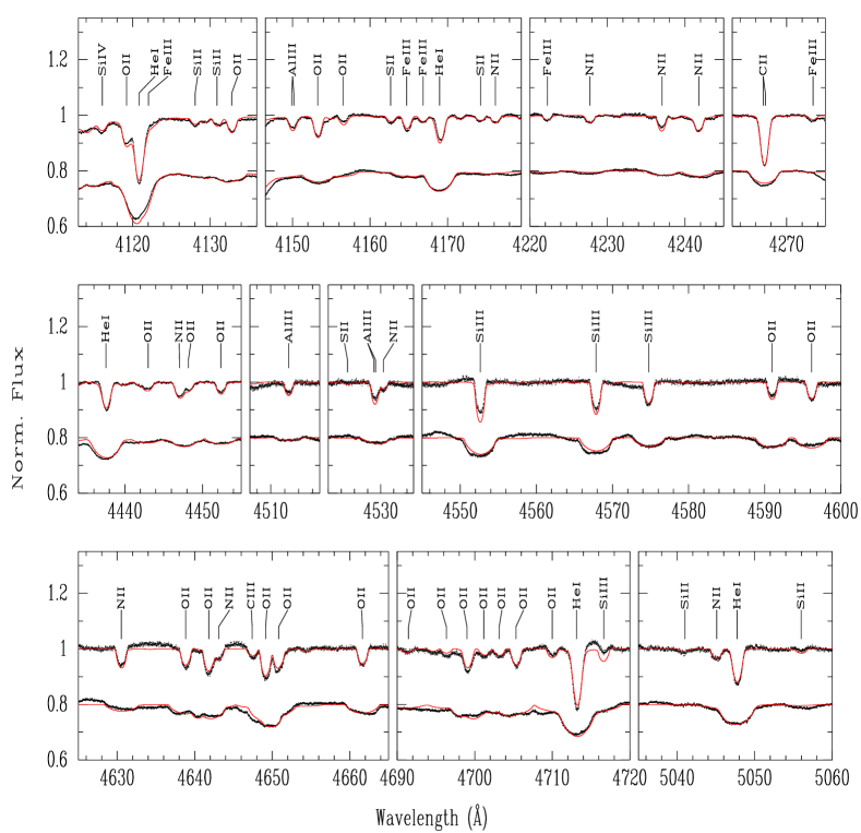
Figure 3: Synthetic (red) vs. separated spectra (black) of components Ca1 (upper) and Cb (lower set of curves).

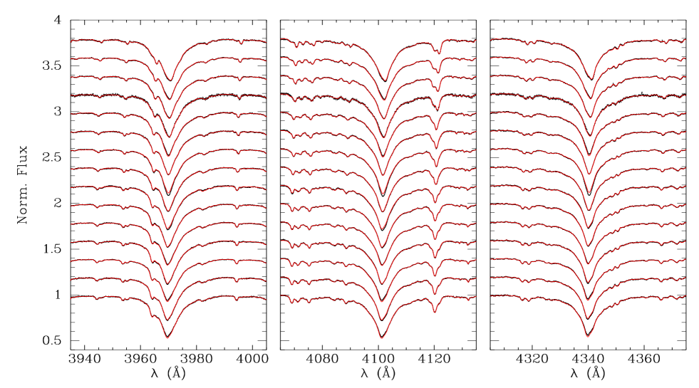
Figure 4: Profiles of several H i lines at different orbital phases. Comparison of composite synthetic spectra (red line) with UVES spectra (small black dots).

Grid-based procedures for the analysis of composite spectra (e.g. Irrgang et al., 2014) could not be applied without prohibitively large extensions of the precomputed grids because of the chemically peculiar nature of the star Cb (see below). Therefore, the line-profile fitting was performed on the basis of dedicated microgrid computations centred around a set of atmospheric parameters for each star, which were refined iteratively. The aim was to derive those parameter combinations for effective temperature $T_{\mathrm{eff}}$, (logarithmic) surface gravity $\log g$, microturbulence $\xi$, projected rotational velocity $v\sin i$, (radial-tangential) macroturbulence $\zeta$, helium abundance $y$ (by number), and individual metal abundances that facilitate an overall good fit to be achieved for i) the disentangled spectra (weak metal lines only) and ii) the observed composite spectra (broad H and He lines, metal lines). The derived parameters should also facilitate the stars to share a common isochrone and a common spectroscopic distance, and lead to consistent flux scaling factors. Many of the parameters are interrelated in the analysis methodology, hence the need for an iterative approach.

In an initial step, we estimated starting values for projected rotational velocities by applying to the separated spectra of the three components the technique introduced by Díaz et al. (2011). Initial values for atmospheric parameters were based on spectral types and considered two additional external constraints: i) the evolutionary age must be the same for all three components, and ii) the mass-ratio $M$(Ca2)/$M$(Ca1) must be consistent with the $q$ value derived from the spectroscopic orbit. When all three stars are considered to belong to the same isochrone, atmospheric parameters and relative fluxes are no longer independent. For fixed temperatures, one single parameter (e.g. age) determines $\log g$ and relative fluxes for all three stars. In these calculations we used the stellar model grids by Ekström et al. (2012). This strategy allowed us to adopt starting gravity values without having individual hydrogen line profiles.

In a second step, both $T_{\mathrm{eff}}$ and $\log g$ were refined on the basis of ionisation equilibria, i.e. all ionisation stages of an observed element have to indicate the same abundance (within the uncertainties), employing narrow He i/ii lines, C ii/iii, O i/ii, Si ii-iv, and S ii/iii. Individual metal lines were fitted using spectral synthesis. Analysing the disentangled spectra required a double-iterative procedure, one on the atmospheric parameters and chemical abundances and another in the scaling factors of the disentangled spectra. New scaling factors were derived from stellar parameters calculated during the analysis of the separated spectra via metal ionisation equilibria. In this instance we relaxed the strict constraint imposed by the theoretical isochrones. From this preliminary analysis, we confirmed that Cb is a He-rich star.

A final check within an iteration step was performed on the observed composite spectra using the refined atmospheric parameters, chemical abundances, and scaling factors. Synthetic composite spectra for particular orbital phases were built by combining the three synthetic spectra of the component stars after shifting by radial velocity, broadening with appropriate rotational and macroturbulent profiles, and scaling according to their relative fluxes. At this stage we were able to include H i and broad He i lines in the analysis. This yielded further estimates for corrections of parameters, for which dedicated synthetic spectra were again computed. We then returned to the investigation of the separated spectra as discussed in the previous paragraph, etc., requiring several iteration steps until no further need for changes in the parameters was found from the spectroscopic analysis, meeting also the additional constraints on consistent ages, spectroscopic distances, the Ca2/Ca1 mass ratio and the flux scaling factors. The procedure turned out to be challenging and time consuming due to the large number of variables, further complicated because of the chemical peculiarities of Cb.

The finally adopted atmospheric and fundamental stellar parameters, and the abundances for the components of HD 164492C are summarised in Table 4. For comparison, chemical abundances as derived from a sample of chemically normal and single early B-type stars in the solar neighbourhood (Nieva & Przybilla, 2012) – the ‘cosmic abundance standard’ (CAS) –, are also given.

Figure 3 shows a selection of spectral lines used in the abundance determination. An overall good to excellent match between the model and the disentangled spectra is obtained. Even so, for some lines the residuals are significantly above the noise level, which is low in the reconstructed spectra (typically 1/400–1/500 of the continuum level). These discrepancies might be a sign of surface chemical spots, although it is also possible that they are remains of the spectral separation process. With the velocity amplitude of star Ca1 being within the width of the line profile of star Cb, the resulting line intensities in the reconstructed spectra of Cb and Ca1 are strongly correlated.

Despite the high signal-to-noise ratio of the separated spectra of the components Ca1 and Cb, the uncertainties in chemical abundances are estimated to be about 0.2 dex. The main error source is the scale factor introduced by the relative fluxes and in the case of Cb the uncertainty in the continuum definition in the region of broad lines or blends. The fitting of Balmer lines was consistent with atmospheric parameters derived from metal lines throughout the orbital period, see Fig. 4.

The star Cb is a He-rich star ($y$ = 0.35$\pm$0.04, i.e. about +0.6 dex above the CAS value) with some metal peculiarities, particularly moderate overabundance of O and Si, and underabundances of C, Ne and Mg. Abundance anomalies are frequently found in He-strong stars as a consequence of the different coupling of individual ions to the stellar wind and due to the formation of chemical inhomogeneities (spots) because of the magnetic field (see e.g. Przybilla et al., 2016), and Cb is not an exception. The star Ca1 has a chemical composition compatible with the CAS, though by trend a slightly more metal-rich composition is indicated.

The faint component Ca2 was assessed only through the disentangled spectrum since its contribution to broad H and He lines is comparatively small making the fitting of composite spectra insensitive to the parameters of this star. However, its narrow metal lines are well reconstructed in the spectral disentangling, though the overall signal-to-noise ratio is low and the uncertainty in its relative flux is large, which affect systematically the line intensities. Moreover, without good neutral or doubly ionised metal lines, it was not possible to derive the surface gravity for this star. Instead, we adopted a value consistent with the age of the more massive stars. As a consequence, we refrain from providing abundance values for Ca2 in Table 4. On the other hand, for any reasonable scale factor the spectrum appears peculiar, the star being apparently a Si-rich Bp type with its effective temperature ranging from about 14 000 to 16 000 K.

6 Physical parameters

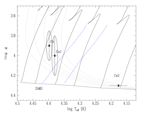
Figure 5: $\log T_{\mathrm{eff}}-\log g$ diagram. Isochrones correspond to Geneva stellar models for rotating stars with $Z=0.014$. Dotted lines are (from left to right) isochrones for log age 6.9, 7.0, 7.1, 7.2, and 7.3. Continuous black lines are (from right to left) stellar tracks for 4, 5, 7, 9, 12, and 15 $M_{\odot}$. The strip marked with the two blue dashed lines corresponds to the stellar models of star Ca1 for which the flux-ratio Ca2-to-Ca1 is 0.16$\pm$0.03, asssuming a temperature 15 000$\pm$1000 K for Ca2.

We fitted the observed spectra assuming that they are formed by three stars of the same age. Figure 5 shows the position of the three companions in the $\log T_{\mathrm{eff}}-\log g$ diagram.

The adopted parameters are listed in the third block of Table 4. The spectroscopic $\log g$ value of stars Cb and Ca1 suggests that they are somewhat evolved within the main-sequence, with an age of $\sim$12-15 Myr according to Geneva models for rotating stars with metallicity $Z=0.014$. Using these masses and the radial velocity curve, we estimate the orbital inclination of the Ca1-Ca2 system to be $i=52\pm 3^{\circ}$.

For the adopted isochrone, assuming star Ca2 is a normal main-sequence star of the same age, the relative flux of star Ca2 would be about 0.040$\pm$0.013. The observed intensity of spectral lines of this star in the composite spectrum, however, suggests a scaling factor $0.061\pm 0.012$. In other words, the intensity of Ca2 lines in the spectrum suggests that stars Ca1 and Cb are somewhat less luminous than found in the spectral analysis. If the relative contribution of flux for star Ca1 is of the order of 0.37, then the intensity of the Ca2 lines suggests that the flux ratio Ca2-to-Ca1 is 0.16$\pm$0.03. The strip between blue lines in Fig. 5 marks the positions of star Ca1 that are consistent with a temperature 15 000$\pm$1000 K for Ca2 and a flux ratio 0.16$\pm$0.03. In short, the spectrum of Ca2, under the assumption of being a normal star of the same age, suggests the system to be somewhat younger, at most 10 Myr.

At periastron the components of the Ca pair are at a separation of about 26 $R_{\odot}$, only 3-4 times larger that the sum of their radii. This is not close enough, however, for the orbit and the rotation velocity of the companions to have suffered significant changes by tidal effects. Calculations with the binary evolution code by Hurley et al. (2002) indicate that no significant evolution of the orbit and rotational velocities would occur until the primary approaches the end of the main-sequence at about 25 Myr. With an eccentricity of $e=0.532$ the pseudo-synchronous rotational period would be 3.994 days. It is interesting that the projected rotation corresponding to the pseudo-synchronous regime, as calculated from the adopted stellar parameters, $51\pm 9$ km s^-1, is in agreement with the observed $v\sin i$ value. In other words, the primary Ca1 seems to be rotating close to the pseudo-synchronous regime, although this would not be caused by tidal forces.

The stellar parameters determined for the components of this multiple system offer the opportunity to calculate the spectroscopic distance modulus. Even though various works have determined the distance to the Trifid Nebula cluster using other stars or properties of the nebula, this issue is still controversial. The high and variable extinction, and mainly the anomalous extinction law has contributed to this. Lynds et al. (1985) reported an extinction law with $R_{V}=5.1$ and estimated a distance of 1.67 kpc. Cambrésy et al. (2011) confirmed this high $R_{V}$ value, but obtain a significantly larger distance. From the colour distribution of stars along the line-of-sight to strongly absorbed regions within the Trifid nebula, they derived the extinction distribution along the line-of-sight and calculated a distance of $2.7\pm 0.5$ kpc to the nebula. A similar value had been obtained from $UBV$ photometry of stars HD 164492A, B, C, and E, by Kohoutek et al. (1999).

Unfortunately none of the stellar components of the multiple system HD164492 is included in the Gaia first data release (Gaia Collaboration, et al., 2016). Parallaxes are available in this catalogue for a few other probable members of the cluster NGC 6514 but the uncertainties are too large ($\sim$50%) for a reliable determination of the distance.

The adopted stellar parameters for the three stars studied in the present paper correspond to a total absolute visual magnitude of $-3.72\pm 0.53$ mag. The apparent $V$ magnitude of this triple system is not well known. The photometric measurements given by Kohoutek et al. (1999) involve also the component HD 164492D. Using the light ratio estimated by the same authors (3.9 at $\lambda=514$ nm), we obtain: $V=8.91$ mag for the integrated magnitude of the system HD 164492C. Assuming a reddening $E(B-V)=0.33\pm 0.03$ mag (Kohoutek et al., 1999, for stars A, B, and C), and $R=5.1$, we derive a distance of $1.55^{+0.45}_{-0.35}$ kpc, supporting the results of Lynds et al. (1985).

7 Spectral variability

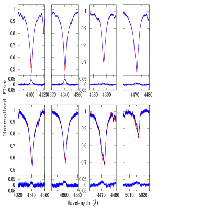
Figure 6: Profile variations of H i and He i lines. Upper panels: comparison of UVES spectra at HJD 2 456 869.5077 (red) and HJD 2 456 919.5607 (blue). Lower panels: comparison of HARPS spectra at HJD 2 457 091.8426 (red) and HJD 2 457 317.5185 (blue). In the lower part of each panel, the difference between the two plotted spectra is shown.

Even though the combination of the reconstructed spectra of the three components reproduces satisfactorily the observed spectra, particularly the metallic lines, some observations show small differences in the core of Balmer lines (see Fig. 4 and 6). In the spectra with strong H lines some strong He lines appear also enhanced, although these variations are always below 1% of the continuum and should be considered as marginal. These line-profile variations are not correlated with the orbital phase of the system Ca1-Ca2. This is shown in Fig.  6 where we compare two UVES spectra (HJD 2 456 869.5077 and 2 456 919.5607) taken at similar orbital phase (near conjunction) but presenting different intensity in H lines and some He lines. Two HARPS spectra exhibiting differences in H and He lines are also shown. In this case the observations were taken on HJD 2 457 091.8426 and 2 457 317.5185, which corresponds to phase $\sim$0.09 (near quadrature with star Ca1 shifted to the red). In some cases these variations are noticeable on consecutive nights, suggesting a short period that might be related with a non-uniform surface of the rotating star Cb. In most of the spectra, however the spectral variations are comparable to the spectrum noise or the continuum uncertainties, making difficult its use for deriving the rotation period.

More than one mechanism could be responsible for these spectral variations. One possible explanation is a temperature variation over the surface of this star. In the temperature range of star Cb, a drop in temperature would strengthen both He and H lines. In chemical peculiar stars, the regions with a great concentration of some particular elements (chemical spots) present a higher opacity, which increases the temperature due to backwarming (see Krtička et al., 2007 for a clear example in a He-strong star). On the other hand, in massive magnetic stars, temperature variations can be related to bright spots that arise due to the lower density (lower optical thickness) of the gas in surface regions with higher magnetic pressure (Cantiello & Braithwaite, 2011).

Besides the mentioned variations in the core of Balmer lines, the line H$\alpha$ shows variable wings which in a few spectra appear in emission. To analyse these variations we subtracted from the UVES spectra synthetic spectra of the three components as calculated in Sect. 5. These difference spectra were used to calculate residual equivalent widths integrating in a wavelength window of 80 Å around H$\alpha$. We find that all UVES spectra exhibit an H$\alpha$ excess in the range 0.5–2.3 Å over the synthetic model, except for the spectrum taken at HJD 2 456 779.9, which has a much stonger emission (3.6 Å), probably due to the contamination by the Herbig Be star (HD 164492D) in the vicinity of HD 164492C. A period search on the sample of fourteen UVES difference spectra shows that these variations might present a periodic behaviour, although the period is not unambiguously determined with the available UVES observations. The most probable periods are 0.557 d, 1.370 d, and 3.68 d. Figure 7 shows the equivalent width curves built with these three periods. The estimated uncertainties are of the order of 0.05 Å. Since FEROS and HARPS are fibre-fed instruments, it is difficult to take into account the background variations. As a results, we do not detect in the spectra obtained with these instruments clear emission variations similar to those detected in UVES spectra.

Figure 7: Flux excess in H$\alpha$ phased with three probable periods.

8 Magnetic fields

Table 5: Logbook of the HARPS spectropolarimetric observations of HD 164492C. Column 1: Heliocentric Julian Date; Column 2: Orbital phase of the subsystem Ca1-Ca2; Column 3: Rotational phase of star Cb using P=1.59689 d and T₀=2 457 001.263; Column 4: Longitudinal magnetic field measured using metallic and He lines; Column 5: Longitudinal magnetic field measured using only metallic lines.

HJD	Orbital	Rotational	$\left<B_{\rm z}\right>_{\rm all}$		$\left<B_{\rm z}\right>_{\rm no\,He}$
	Phase	Phase	[G]		[G]
2 456 445.7946	0.5559	0.1548	615$\pm$	22	309$\pm$	64
2 456 446.7934	0.6355	0.7803	351$\pm$	24	203$\pm$	65
2 456 770.7700	0.4808	0.6606	$-$52$\pm$	16	$-$78$\pm$	41
2 456 771.7850	0.5618	0.2963	11$\pm$	15	18$\pm$	45
2 457 091.8426	0.0944	0.7225	$-$72$\pm$	27	$-$27$\pm$	83
2 457 092.8282	0.1730	0.3397	48$\pm$	26	$-$89$\pm$	77
2 457 093.8478	0.2544	0.9782	404$\pm$	22	419$\pm$	56
2 457 094.8153	0.3316	0.5840	325$\pm$	32	42$\pm$	67
2 457 178.6948	0.0231	0.1110	784$\pm$	20	467$\pm$	37
2 457 179.7426	0.1067	0.7671	$-$46$\pm$	36	228$\pm$	76
2 457 317.5185	0.0977	0.0450	905$\pm$	37	406$\pm$	62

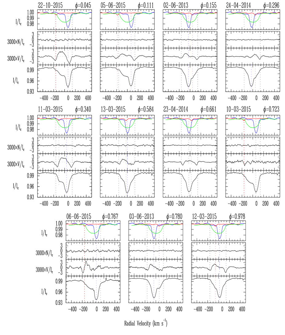
Figure 8: $I$, $V$, and $N$ SVD profiles obtained for the system HD 164492C on eleven different epochs using a line mask including all lines. In the upper panel we present the SVD Stokes $I$ line profiles for each component at different positions in velocity space according to their radial velocity shifts due to orbital movement. The $V$ and $N$ profiles were expanded by the indicated factor for better visibility. Note that the plots are ordered according to rotational phase and not to increasing Julian date.

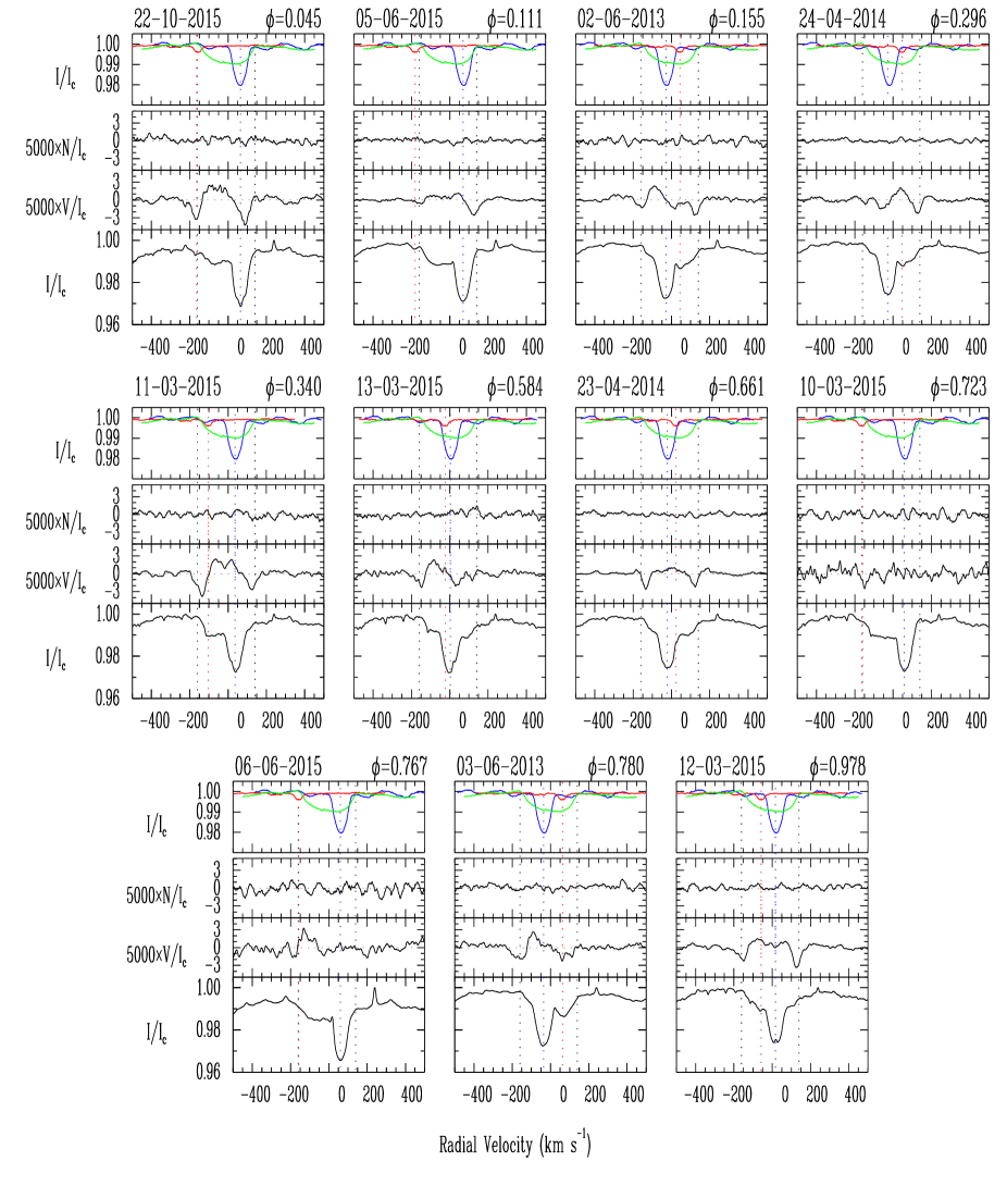
Figure 9: The same as in Fig. 8 but using exclusively metal lines.

The reduction and magnetic field measurements were carried out using dedicated software packages developed for the treatment of high-resolution spectropolarimetric data. The spectrum reduction and calibration was performed using the HARPS data reduction pipeline available at the ESO 3.6-m telescope in Chile. The normalisation of the spectra to the continuum level consisted of several steps described in detail by Hubrig et al. (2013). The software package used to study the magnetic field in HD 164492C, the so-called multi-line Singular Value Decomposition (SVD) method for Stokes profile reconstruction was recently introduced by Carroll et al. (2012). More details on the basic idea of SVD can be found in Carroll et al. (2009). The results of our magnetic field measurements, those for the line list including all lines and the line list excluding He lines, are presented in Table 5, where we also collect information about the heliocentric Julian date for the middle of the exposure, and the rotational phase assuming a period of 1.5969 d (see below).

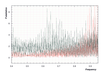
Figure 10: Periodogram for the mean longitudinal magnetic field measured without He lines. The peak at 0.6262 d^-1 corresponds to a period of 1.5969 d. The window function is plotted in red.

The resulting mean Stokes $I$, Stokes $V$, and Null profiles obtained by using the SVD method with 109 metallic lines in the line mask and with the line mask including He lines (125 lines) are presented in Figs. 8 and 9. Null polarisation spectra were calculated by combining the subexposures in such a way that polarisation cancels out. The line mask was constructed using the VALD database (e.g.  Kupka et al., 2000). The mean longitudinal magnetic field was estimated from the SVD reconstructed Stokes $V$ and $I$ using the centre-of-gravity method (see e.g. Carroll & Strassmeier 2014). The velocity window used in these measurement was about 400 km s^-1 wide, which includes all three components in all phases. We note that due to the fact that HD 164492C is a hierarchical triple system and all three components remain blended in all observed spectra, the estimation of the magnetic field can only be done assuming that HD 164492C is a single star. A definite detection of a mean longitudinal magnetic field, $\left<B_{\rm z}\right>$, with a false alarm probability (FAP) smaller than $10^{-6}$, was achieved on all epochs apart from the observation on HJD 2 457 091.8426 (orbital phase 0.09) where a marginal detection was achieved for the line mask including all lines, and no detection for the line mask including exclusively metal lines. The analysis of the diagnostic Null profiles showed non-detections at all phases apart from the same epoch at the orbital phase 0.09 where we achieve a marginal detection with FAP of about $2\times 10^{-5}$ for the same line mask with metal lines.

In the framework of our ESO Large Programme 191.D-0255, the first spectropolarimetric observations of HD 164492C were carried out in 2013 with the low-resolution FORS 2 spectrograph and were complemented in the same year by two observations using HARPS in spectropolarimetric mode (Hubrig et al., 2014). While FORS 2 observations indicated a strong longitudinal magnetic field of about 500–600 G, the HARPS observations revealed that HD 164492C could not be considered a single star as it possessed one or two companions. Given the complex configuration and shape of the Stokes profiles, it was also impossible to conclude exactly which components possessed a magnetic field. The detection of a significant Stokes $V$ signature in the SVD and LSD profiles at about $-100$ km s^-1 and $+150$ km s^-1 from the line core of the primary suggested that more than one component might hold a magnetic field. On the other hand, assuming that HD 164492C is a single star, we obtained results very similar to those obtained with FORS 2: between 500 and 700 G for the first HARPS observing night, and between 400 and 600 G for the second HARPS night.

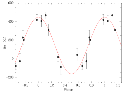
Figure 11: Magnetic field curve calculated with a period of 1.5969 days. The plotted values correspond to the longitudinal magnetic field measured using metallic lines.

Since 2013 we were able to acquire nine additional HARPS spectropolarimetric observations. Admittedly, even having at our disposal observations at eleven epochs, the interpretation of the temporal behaviour of the Stokes $V$ profiles is a challenging task because the line profiles of the three stars overlap in all orbital phases. In fact, the radial velocity amplitude of the star Ca1, the primary of the spectroscopic binary, is smaller than the projected rotational velocity of the star Cb, which has a similar spectral type. The radial velocity amplitude of the component Ca2 is larger, but still overlaps the wings of the SVD line profile of the rapidly rotating component Cb. We note, however, that at several epochs (for example on 02-06-2013 and 24-04-2014, corresponding both to the orbital phase 0.56) we observe significant features in the Stokes $V$ profiles that are located in the velocity space far from the positions corresponding to stars Ca1 and Ca2. These features can only be attributed to the star Cb. It is possible therefore, to identify the spectroscopic component Cb as a star possessing a magnetic field. This is in line with it being a He-rich star. The group of He-peculiar stars are as a rule strongly magnetic (Borra & Landstreet, 1979). Given the rather fast changes in the shape of Zeeman features over consecutive nights, we expect that the rotation period of this component is rather short. It is obvious that the magnetic character of the star Ca1 cannot be addressed as long as the magnetic variations of the star Cb are not modelled. Still, due to the severe distortion of the Zeeman features at the positions corresponding to the red or blue wing of the Stokes $I$ profile of the component Cb at some epochs, we cannot exclude that also the star Ca1 possesses a magnetic field. Indeed, sometimes only the blue part of the Zeeman feature is visible (for example at HJD 2 457 091.8426 - rotational phase 0.72, or HJD 2 457 179.7426 - rotational phase 0.77) and sometimes only the red part of the Zeeman feature (for example at HJD 2 456 771.7850 - rotational phase 0.30). In the working hypothesis assuming that Cb is the only magnetic star and shows a dipole structure, for all observational aspects of the dipole configuration, i.e. either close to the magnetic poles or close to the magnetic equator, we would always expect a certain symmetry in the appearance of the Zeeman features relative to the line centre of the component Cb, unless strong contrast chemical inhomogeneities are present on the surface. Interestingly, since He is especially strong in the component Cb, Zeeman features appear less noisy in the Stokes $V$ spectra obtained including He lines at the orbital phases mentioned above. As for the star Ca2, we can conclude that its low relative contribution to the total flux (5-7% of the total light) makes its potential magnetic features (because of its probable BpSi type) to be virtually undetectable.

From the estimated stellar parameters and the projected rotational velocities, upper limits for the rotational period of the stars can be obtained. In the case of the star Cb, assuming a radius of $6.3\,R_{\odot}$ leads to a period of less than about 2.3 days.

In order to search for rotational modulations of the magnetic field, we performed a periodicity analysis of the mean longitudinal magnetic field measurements. Figure 10 shows the periodogram corresponding to measurements obtained without the He lines. A few probable periods appear in the range 1.4–1.6 days (frequencies of $0.62-0.72$ d^-1). The highest peak corresponds to $P=1.5969$ d. Figure 11 shows the magnetic measurements using metallic lines phased with this period.

On the other hand, as mentioned in Sect. 7, the line profiles of H$\alpha$ in UVES spectra exhibit excess of emission indicating periodicity with the probable periods of 0.557 d, 1.370 d, and 3.68 d. It is possible that the appearance of the broad emission profiles is related to the presence of the magnetosphere around the He-rich Cb component where stellar wind is forced to corotate with the star up to the Alfvén radius. Thus, the periodic variability of the emission in the H$\alpha$ line profile can be probably related to the rotational period of this component.

Figure 12: Variation of the Stokes $V$ LSD profiles of HD 164492C (all three components included) with respect to the rotational phases calculated with $P=1.370$ d and $P=1.5969$ d. In each panel, the $V/I_{c}$ profiles are scaled by a factor 50 and shifted according to the rotational phase $\phi$.

In Figure 12 we present the Stokes $V$ profiles obtained for the line mask including all lines ordered according to rotational phases calculated with periods 1.370 and 1.597 days. The apparent resemblance of Stokes $V$ Zeeman profiles in observations obtained in similar phases suggests that the period of 1.37 day can also be considered as a tentative rotational period of the component Cb. Our magnetic field measurements, however, do not show a coherent curve if this period is used to phase the data. We cannot, therefore, give a definite conclusion about the rotational period with the present observational material.

9 Conclusions

HD 164492C is a hierarchical triple system, which on its own is probably a member of a larger multiple system. Two early-B type stars of similar masses (Ca1 and Cb) are bound in a wide binary system with a separation of the order of 100 AU (González & Veramendi, 2016). One of these stars (star Ca1) has a close companion in an orbit with a period of 12.5 d. The radial velocity of the tertiary star Cb coincides within uncertainties with the centre-of-mass velocity of the pair Ca12 and with the velocity of the nebula. The velocity variations due to the orbital motion of the pair Cb-Ca are not detectable, since with the estimated masses and projected separation, the period would be at least 100 times longer than the timespan of our observations.

Star Cb is the most massive star in the system with a mass of about 11 $M_{\odot}$. It is the apparently fastest rotator of the system and its surface gravity suggests that it is close to the middle of its main-sequence lifetime. It is chemically peculiar, exhibiting a strong overabundance of helium ($y$ = 0.35, or about +0.6 dex over the CAS value). The spectroscopic pair is formed by a 10 $M_{\odot}$ primary and a 4 $M_{\odot}$ secondary in an eccentric 12.5 d orbit. The least massive star is probably a BpSi star.

The distance to the Trifid nebula is not well known and previous determinations range from 1.7 kpc to 2.7 kpc. We have derived the spectroscopic distance modulus for the triple star HD 164492C, member of the Trifid nebula stellar association, and obtained a value of 1.5 kpc, which clearly supports the short distance scale. Similar results are found from the spectroscopic distance modulus of other nearby stars (Przybilla et al., in preparation). The spectral morphology is consistent with three main-sequence stars of at least 10 Myr. The dynamical age of the Trifid nebula is about 0.3 Myr (Cernicharo et al., 1998), while the most accepted age for the first-generation stars, to which the central O-star HD 164492A belongs, is of the order of 1 Myr (Torii et al., 2011). In a future paper (Przybilla et al., in preparation) we will address the problem of the age of the stellar population of M20 in further detail, but we mention here that the spectral analysis of several stars in the region would suggest that besides the young population, with spectral morphology consistent with 1 Myr, there are a few other stars that might be on the same isochrone as HD 164492C.

We confirm the presence of a magnetic field in the triple system HD 164492C and identified the He-strong tertiary companion Cb as being the magnetic star. The detection of the magnetic field in this chemically peculiar star confirms the hypothesis that He-strong stars are a hot extension of the Ap phenomenon (e.g. Borra & Landstreet, 1979). However, the observed asymmetry of Zeeman features indicates that the magnetic field cannot be described exclusively by a rotating dipole structure on the surface of the Cb component: either the star Ca1 is also magnetic or the geometry of the magnetic field of the star Cb is relatively complex. Our variability analyses of the longitudinal magnetic field and the behaviour of the emission excess in the H$\alpha$ lines suggest tentative magnetic periods of 1.6 d and 1.4 d. These values, however, should be confirmed by additional observations.

While this paper was being refereed, Wade et al. (2016) published a study on the same object. This work makes use of most of the observations presented in this paper along with an additional series of spectropolarimetric observations obtained with ESPaDOnS at the Canada-France-Hawaii Telescope. The spectroscopic orbit obtained by these authors agrees with the one presented here. Their estimated stellar parameters are also compatible, although their parameters are not calculated solely from the observational data, but through an assumption of distance and age of the Trifid Nebula. Based on 23 magnetic field measurements they derive a rotational period of 1.3699 d and obtained inclination and obliquity under the assumption of the dipolar oblique rotator model.

References

- Becker (1998) Becker S. R., 1998, in Howarth I., ed., Astronomical Society of the Pacific Conference Series Vol. 131, Properties of Hot Luminous Stars. p. 137
- Becker & Butler (1988) Becker S. R., Butler K., 1988, A&A, 201, 232
- Borra & Landstreet (1979) Borra E. F., Landstreet J. D., 1979, ApJ, 228, 809
- Borra et al. (1982) Borra E. F., Landstreet J. D., Mestel L., 1982, ARA&A, 20, 191
- Butler & Giddings (1985) Butler K., Giddings J. R., 1985, Newsletter of Analysis of Astronomical Spectra, 9
- Cambrésy et al. (2011) Cambrésy L., Rho J., Marshall D. J., Reach W. T., 2011, A&A, 527, A141
- Cantiello & Braithwaite (2011) Cantiello M., Braithwaite J., 2011, A&A, 534, A140
- Carroll & Strassmeier (2014) Carroll T. A., Strassmeier K. G., 2014, A&A, 563, A56
- Carroll et al. (2009) Carroll T. A., Kopf M., Strassmeier K. G., Ilyin I., 2009, in Strassmeier K. G., Kosovichev A. G., Beckman J. E., eds, IAU Symposium Vol. 259, Cosmic Magnetic Fields: From Planets, to Stars and Galaxies. pp 633–644 (arXiv:0903.1008), doi:10.1017/S1743921309031469
- Carroll et al. (2012) Carroll T. A., Strassmeier K. G., Rice J. B., Künstler A., 2012, A&A, 548, A95
- Cernicharo et al. (1998) Cernicharo J., et al., 1998, Science, 282, 462
- Díaz et al. (2011) Díaz C. G., González J. F., Levato H., Grosso M., 2011, A&A, 531, A143
- Ekström et al. (2012) Ekström S., et al., 2012, A&A, 537, A146
- Ferrario et al. (2009) Ferrario L., Pringle J. E., Tout C. A., Wickramasinghe D. T., 2009, MNRAS, 400, L71
- Ferrario et al. (2015) Ferrario L., Melatos A., Zrake J., 2015, Space Sci. Rev., 191, 77
- Gaia Collaboration, et al. (2016) Gaia Collaboration, Brown A. G. A., Vallenari A., Prusti T., de Bruijne J. H. J., Mignard F., et al. 2016, A&A, special Gaia volume, special volume, 1
- Giddings (1981) Giddings J. R., 1981, PhD thesis, , University of London, (1981)
- González & Levato (2006) González J. F., Levato H., 2006, A&A, 448, 283
- González & Veramendi (2016) González J. F., Veramendi M. E., 2016, Boletin de la Asociacion Argentina de Astronomia La Plata Argentina, 58, 105
- Grunhut & Wade (2013) Grunhut J. H., Wade G. A., 2013, in Pavlovski K., Tkachenko A., Torres G., eds, EAS Publications Series Vol. 64, EAS Publications Series. pp 67–74, doi:10.1051/eas/1364009
- Hubrig et al. (2013) Hubrig S., Ilyin I., Schöller M., Lo Curto G., 2013, Astronomische Nachrichten, 334, 1093
- Hubrig et al. (2014) Hubrig S., et al., 2014, A&A, 564, L10
- Hurley et al. (2002) Hurley J. R., Tout C. A., Pols O. R., 2002, MNRAS, 329, 897
- Irrgang et al. (2014) Irrgang A., Przybilla N., Heber U., Böck M., Hanke M., Nieva M.-F., Butler K., 2014, A&A, 565, A63
- Kohoutek et al. (1999) Kohoutek L., Mayer P., Lorenz R., 1999, A&AS, 134, 129
- Krtička et al. (2007) Krtička J., Mikulášek Z., Zverko J., Žižńovský J., 2007, A&A, 470, 1089
- Kupka et al. (2000) Kupka F. G., Ryabchikova T. A., Piskunov N. E., Stempels H. C., Weiss W. W., 2000, Baltic Astronomy, 9, 590
- Kurucz (1993) Kurucz R., 1993, ATLAS9 Stellar Atmosphere Programs and 2 km/s grid. Kurucz CD-ROM No. 13. Cambridge, Mass.: Smithsonian Astrophysical Observatory, 1993., 13
- Lanz & Hubeny (2007) Lanz T., Hubeny I., 2007, ApJS, 169, 83
- Lynds et al. (1985) Lynds B. T., Canzian B. J., Oneil Jr. E. J., 1985, ApJ, 288, 164
- Morel & Butler (2008) Morel T., Butler K., 2008, A&A, 487, 307
- Morel et al. (2006) Morel T., Butler K., Aerts C., Neiner C., Briquet M., 2006, A&A, 457, 651
- Morel et al. (2014) Morel T., et al., 2014, The Messenger, 157, 27
- Morel et al. (2015) Morel T., et al., 2015, in Meynet G., Georgy C., Groh J., Stee P., eds, IAU Symposium Vol. 307, New Windows on Massive Stars. pp 342–347 (arXiv:1408.2100), doi:10.1017/S1743921314007054
- Moss (2001) Moss D., 2001, in Mathys G., Solanki S. K., Wickramasinghe D. T., eds, Astronomical Society of the Pacific Conference Series Vol. 248, Magnetic Fields Across the Hertzsprung-Russell Diagram. p. 305
- Nieva & Przybilla (2006) Nieva M. F., Przybilla N., 2006, ApJL, 639, L39
- Nieva & Przybilla (2007) Nieva M. F., Przybilla N., 2007, A&A, 467, 295
- Nieva & Przybilla (2008) Nieva M. F., Przybilla N., 2008, A&A, 481, 199
- Nieva & Przybilla (2012) Nieva M.-F., Przybilla N., 2012, A&A, 539, A143
- Nieva & Simón-Díaz (2011) Nieva M.-F., Simón-Díaz S., 2011, A&A, 532, A2
- Przybilla (2005) Przybilla N., 2005, A&A, 443, 293
- Przybilla & Butler (2001) Przybilla N., Butler K., 2001, A&A, 379, 955
- Przybilla & Butler (2004) Przybilla N., Butler K., 2004, ApJ, 609, 1181
- Przybilla et al. (2000) Przybilla N., Butler K., Becker S. R., Kudritzki R. P., Venn K. A., 2000, A&A, 359, 1085
- Przybilla et al. (2001) Przybilla N., Butler K., Becker S. R., Kudritzki R. P., 2001, A&A, 369, 1009
- Przybilla et al. (2011) Przybilla N., Nieva M.-F., Butler K., 2011, Journal of Physics Conference Series, 328, 012015
- Przybilla et al. (2013) Przybilla N., Nieva M. F., Irrgang A., Butler K., 2013, in Alecian G., Lebreton Y., Richard O., Vauclair G., eds, EAS Publications Series Vol. 63, EAS Publications Series. pp 13–23, doi:10.1051/eas/1363002
- Przybilla et al. (2016) Przybilla N., et al., 2016, A&A, 587, A7
- Sota et al. (2014) Sota A., Maíz Apellániz J., Morrell N. I., Barbá R. H., Walborn N. R., Gamen R. C., Arias J. I., Alfaro E. J., 2014, ApJs, 211, 10
- Stasińska (2009) Stasińska G., 2009, What can emission lines tell us?. p. 1
- Torii et al. (2011) Torii K., et al., 2011, ApJ, 738, 46
- Vrancken et al. (1996) Vrancken M., Butler K., Becker S. R., 1996, A&A, 311, 661
- Wade et al. (2016) Wade G. A., et al., 2016, preprint, (arXiv:1610.02585)
- Yusef-Zadeh et al. (2005) Yusef-Zadeh F., Biretta J., Geballe T. R., 2005, AJ, 130, 1171