Semantic Annotation for Microblog Topics
Using Wikipedia Temporal Information

Abstract

Trending topics in microblogs such as Twitter are valuable resources to understand social aspects of real-world events. To enable deep analyses of such trends, semantic annotation is an effective approach; yet the problem of annotating microblog trending topics is largely unexplored by the research community. In this work, we tackle the problem of mapping trending Twitter topics to entities from Wikipedia. We propose a novel model that complements traditional text-based approaches by rewarding entities that exhibit a high temporal correlation with topics during their burst time period. By exploiting temporal information from the Wikipedia edit history and page view logs, we have improved the annotation performance by 17-28%, as compared to the competitive baselines.

1 Introduction

With the proliferation of microblogging and its wide influence on how information is shared and digested, the studying of microblog sites has gained interest in recent NLP research. Several approaches have been proposed to enable a deep understanding of information on Twitter. An emerging approach is to use semantic annotation techniques, for instance by mapping Twitter information snippets to canonical entities in a knowledge base or to Wikipedia [Meij et al., 2012, Guo et al., 2013], or by revisiting NLP tasks in the Twitter domain [Owoputi et al., 2013, Ritter et al., 2011]. Much of the existing work focuses on annotating a single Twitter message (tweet). However, information in Twitter is rarely digested in isolation, but rather in a collective manner, with the adoption of special mechanisms such as hashtags. When put together, the unprecedentedly massive adoption of a hashtag within a short time period can lead to bursts and often reflect trending social attention. Understanding the meaning of trending hashtags offers a valuable opportunity for various applications and studies, such as viral marketing, social behavior analysis, recommendation, etc. Unfortunately, the task of hashtag annotation has been largely unexplored so far.

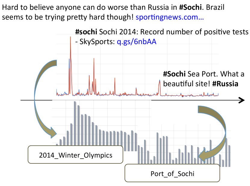
Figure 1: Example of trending hashtag annotation. During the 2014 Winter Olympics, the hashtag ‘#sochi’ had a different meaning.

In this paper, we study the problem of annotating trending hashtags on Twitter by entities derived from Wikipedia. Instead of establishing a static semantic connection between hashtags and entities, we are interested in dynamically linking the hashtags to entities that are closest to the underlying topics during burst time periods of the hashtags. For instance, while ‘#sochi’ refers to a city in Russia, during February 2014, the hashtag was used to report the 2014 Winter Olympics (cf. Figure 1). Hence, it should be linked more to Wikipedia pages related to the event than to the location.

Compared to traditional domains of text (e.g., news articles), annotating hashtags poses additional challenges. Hashtags’ surface forms are very ad-hoc, as they are chosen not in favor of the text quality, but by the dynamics in attention of the large crowd. In addition, the evolution of the semantics of hashtags (e.g., in the case of ‘#sochi’) makes them more ambiguous. Furthermore, a hashtag can encode multiple topics at once. For example, in March 2014, ‘#oscar’ refers to the 86th Academy Awards, but at the same time also to the Trial of Oscar Pistorius. Sometimes, it is difficult even for humans to understand a trending hashtag without knowledge about what was happening with the related entities in the real world.

In this work, we propose a novel solution to these challenges by leveraging temporal knowledge about entity dynamics derived from Wikipedia. We hypothesize that a trending hashtag is associated with an increase in public attention to certain entities, and this can also be observed on Wikipedia. As in Figure 1, we can identify 2014 Winter Olympics as a prominent entity for ‘#sochi’ during February 2014, by observing the change of user attention to the entity, for instance via the page view statistics of Wikipedia articles. We exploit both Wikipedia edits and page views for annotation. We also propose a novel learning method, inspired by the information spreading nature of social media such as Twitter, to suggest the optimal annotations without the need for human labeling. In summary:

• We are the first to combine the Wikipedia edit history and page view statistics to overcome the temporal ambiguity of Twitter hashtags.

• We propose a novel and efficient learning algorithm based on influence maximization to automatically annotate hashtags. The idea is generalizable to other social media sites that have a similar information spreading nature.

• We conduct thorough experiments on a real-world dataset and show that our system can outperform competitive baselines by 17-28%.

2 Related Work

Entity Linking in Microblogs

The task of semantic annotation in microblogs has been recently tackled by different methods, which can be divided into two classes, i.e., content-based and graph-based methods. While the content-based methods [Meij et al., 2012, Guo et al., 2013, Fang and Chang, 2014] consider tweets independently, the graph-based methods [Cassidy et al., 2012, Liu et al., 2013] use all related tweets (e.g., posted by a user) together. However, most of them focus on entity mentions in tweets. In contrast, we take into account hashtags which reflect the topics discussed in tweets, and leverage external resources from Wikipedia (in particular, the edit history and page view logs) for semantic annotation.

Analysis of Twitter Hashtags

In an attempt to understand the user interest dynamics on Twitter, a rich body of work analyzes the temporal patterns of popular hashtags [Lehmann et al., 2012, Naaman et al., 2011, Tsur and Rappoport, 2012]. Few works have paid attention to the semantics of hashtags, i.e., to the underlying topics conveyed in the corresponding tweets. Recently, ?) attempt to segment a hashtag and link each of its tokens to a Wikipedia page. However, the authors only aim to retrieve entities directly mentioned within a hashtag, which are very few in practice. The external information derived from the tweets is largely ignored. In contrast, we exploit both context information from the microblog and Wikipedia resources.

Event Mining Using Wikipedia

Recently some works exploit Wikipedia for detecting and analyzing events on Twitter [Osborne et al., 2012, Tolomei et al., 2013, Tran et al., 2014]. However, most of the existing studies focus on the statistical signals of Wikipedia (such as the edit or page view volumes). We are the first to combine the content of the Wikipedia edit history and the magnitude of page views to handle trending topics on Twitter.

3 Framework

Preliminaries

We refer to an entity (denoted by $e$) as any object described by a Wikipedia article (ignoring disambiguation, lists, and redirect pages). The number of times an entity’s article has been requested is called the entity view count. The text content of the article is denoted by $C(e)$. In this work, we choose to study hashtags at the daily level, i.e., from the timestamps of tweets we only consider their creation day. A hashtag is called trending at a time point (a day) if the number of tweets where it appears is significantly higher than that on other days. There are many ways to detect such trendings. [Lappas et al., 2009, Lehmann et al., 2012]. Each trending hashtag has one or multiple burst time periods, surrounding the trending day, where the users’ interest in the underlying topic remains stronger than in other periods. We denote with $T(h)$ (or $T$ for short) one hashtag burst time period, and with $D_{T}(h)$ the set of tweets containing the hashtag $h$ created during $T$.

Task Definition

Given a trending hashtag $h$ and the burst time period $T$ of $h$, identify the top-$k$ most prominent entities to describe $h$ during $T$.

It is worth noting that not all trending hashtags are mapable to Wikipedia entities, as the coverage of topics in Wikipedia is much lower than on Twitter. This is also the limitation of systems relying on Wikipedia such as entity disambiguation, which can only disambiguate popular entities and not the ones in the long tail. In this study, we focus on the precision and the popular trending hashtags, and leave the improvement of recall to future work.

Overview

We approach the task in three steps. The first step is to identify all entity candidates by checking surface forms of the constituent tweets of the hashtag. In the second step, we compute different similarities between each candidate and the hashtag, based on different types of contexts, which are derived from either side (Wikipedia or Twitter). Finally, we learn a unified ranking function for each (hashtag, entity) pair and choose the top-$k$ entities with the highest scores. The ranking function is learned through an unsupervised model and needs no human-defined labels.

3.1 Entity Linking

The most obvious resource to identify candidate entities for a hashtag is via its tweets. We follow common approaches that use a lexicon to match each textual phrase in a tweet to a potential entity set [Shen et al., 2013, Fang and Chang, 2014]. Our lexicon is constructed from Wikipedia page titles, hyperlink anchors, redirects, and disambiguation pages, which are mapped to the corresponding entities. As for the tweet phrases, we extract all $n$-grams ($n\leq 5$) from the input tweets within $T$. We apply the longest-match heuristic [Meij et al., 2012]: We start with the longest $n$-grams and stop as soon as the entity set is found, otherwise we continue with the smaller constituent $n$-grams.

Candidate Set Expansion

While the lexicon-based linking works well for single tweets, applying it on the hashtag level has subtle implications. Processing a huge amount of text, especially during a hashtag burst time period, incurs expensive computational costs. Therefore, to guarantee a good recall in this step while still maintaining feasible computation, we apply entity linking only on a random sample of the complete tweet set. Then, for each candidate entity $e$, we include all entities whose Wikipedia article is linked with the article of $e$ by an outgoing or incoming link.

3.2 Measuring Entity–Hashtag Similarities

To rank the entity by prominence, we measure the similarity between each candidate entity and the hashtag. We study three types of similarities:

Mention Similarity

This measure relies on the explicit mentions of entities in tweets. It assumes that entities directly linked from more prominent anchors are more relevant to the hashtag. It is estimated using both statistics from Wikipedia and tweet phrases, and turns out to be surprisingly effective in practice [Fang and Chang, 2014].

Context Similarity

For entities that are not directly linked to mentions (the mention similarity is zero) we exploit external resources instead. Their prominence is perceived by users via external sources, such as web pages linked from tweets, or entity home pages or Wikipedia pages. By exploiting the content of entities from these external sources, we can complement the explicit similarity metrics based on mentions.

Temporal Similarity

The two measures above rely on the textual representation and are degraded by the linguistic difference between the two platforms. To overcome this drawback, we incorporate the temporal dynamics of hashtags and entities, which serve as a proxy to the change of user interests towards the underlying topics [Ciglan and Nørvåg, 2010]. We employ the correlation between the times series of hashtag adoption and the entity view as the third similarity measure.

3.3 Ranking Entity Prominence

While each similarity measure captures one evidence of the entity prominence, we need to unify all scores to obtain a global ranking function. In this work, we propose to combine the individual similarities using a linear function:

$$f(e,h)=\alpha f_{m}(e,h)+\beta f_{c}(e,h)+\gamma f_{t}(e,h)$$ (1)

where $\alpha,\beta,\gamma$ are model weights and $f_{m},f_{c},f_{t}$ are the similarity measures based on mentions, context, and temporal information, respectively, between the entity $e$ and the hashtag $h$. We further constrain that $\alpha+\beta+\gamma=1$, so that the ranking scores of entities are normalized between $0$ and $1$, and that our learning algorithm is more tractable. The algorithm, which automatically learns the parameters without the need of human-labeled data, is explained in detail in Section 5.

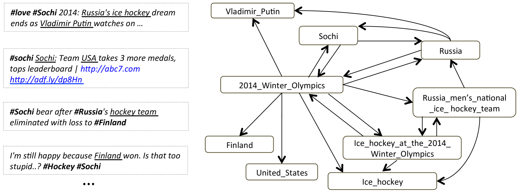
Figure 2: Excerpt of tweets about ice hockey results in the 2014 Winter Olympics (left), and the observed linking process between time-aligned revisions of candidate Wikipedia entities (right). Links come more from prominent entities to marginal ones to provide background, or more context for the topics. Thus, starting from prominent entities, we can reach more entities in the graph of candidate entities

4 Similarity Measures

We now discuss in detail how the similarity measures between hashtags and entities are computed.

4.1 Link-based Mention Similarity

The similarity of an entity with one individual mention in a tweet can be interpreted as the probabilistic prior in mapping the mention to the entity via the lexicon. One common way to estimate the entity prior exploits the anchor statistics from Wikipedia links, and has been proven to work well in different domains of text. We follow this approach and define $LP(e|m)=\frac{|l_{m}(e)|}{\sum_{m^{\prime}}|l_{m^{\prime}}(e)|}$ as the link prior of the entity $e$ given a mention $m$, where $l_{m}(e)$ is the set of links with anchor $m$ that point to $e$. The mention similarity $f_{m}$ is measured as the aggregation of link priors of the entity $e$ over all mentions in all tweets with the hashtag $h$:

$$f_{m}(e,h)=\sum_{m}(LP(e|m)\cdot q(m))$$ (2)

where $q(m)$ is the frequency of the mention $m$ over all mentions of $e$ in all tweets of $h$.

4.1.1 Context Similarity

To compute $f_{c}$, we first construct the contexts for hashtags and entities. The context of a hashtag is built by extracting all words from its tweets. We tokenize and parse the tweets’ part-of-speech tags [Owoputi et al., 2013], and remove words of Twitter-specific tags (e.g., @-mentions, URLs, emoticons, etc.). Hashtags are normalized using the word breaking method by ?).

The textual context of an entity is extracted from its Wikipedia article. One subtle aspect is that the articles are not created at once, but are incrementally updated over time in accordance with changing information about entities. Texts added in the same time period of a trending hashtag contribute more to the context similarity between the entity and the hashtag. Based on this observation, we use the Wikipedia revision history – an archive of all revisions of Wikipedia articles – to calculate the entity context. We collect the revisions of articles during the time period $T$, plus one day to acknowledge possible time lags. We compute the difference between two consecutive revisions, and extract only the added text snippets. These snippets are accumulated to form the temporal context of an entity $e$ during $T$, denoted by $C_{T}(e)$. The distribution of a word $w$ for the entity $e$ is estimated by a mixture between the probability of generating $w$ from the temporal context and from the general context $C(e)$ of the entity:

$$\hat{P}(w|e)=\lambda\hat{P}(w|M_{C_{T}(e)})+(1-\lambda)\hat{P}(w|M_{C(e)})$$

where $M_{C_{T}(e)}$ and $M_{C(e)}$ are the language models of $e$ based on $C_{T}(e)$ and $C(e)$, respectively. The probability $\hat{P}(w|M_{C(e)})$ can be regarded as corresponding to the background model, while $\hat{P}(w|M_{C_{T}(e)})$ corresponds to the foreground model in traditional language modeling settings. Here we use a simple maximum likelihood estimation to estimate these probabilities: $\hat{P}(w|M_{C(e)})=\frac{tf_{w,c}}{|C(e)|}$ and $\hat{P}(w|M_{C_{T}(e)})=\frac{tf_{w,c_{T}}}{|C_{T}(e)|}$, where $tf_{w,c}$ and $tf_{w,c_{T}}$ are the term frequencies of $w$ in the two text sources of $C(e)$ and $C_{T}(e)$, respectively, and $|C(e)|$ and $|C_{T}(e)|$ are the lengths of the two texts, respectively. We use the same estimation for tweets: $\hat{P}(w|h)=\frac{tf_{w,D(h)}}{|D(h)|}$, where $D(h)$ is the concatenated text of all tweets of $h$ in $T$. We use and normalize the Kullback-Leibler divergence to compare the distributions over all words appearing both in the Wikipedia contexts and the tweets:

$$KL(e\;\|\;h) =\sum_{w}\hat{P}(w|e)\cdot\frac{\hat{P}(w|e)}{\hat{P}(w|h)}$$

$$f_{c}(e,h) =e^{-KL(e\;\|\;h)}$$ (3)

4.1.2 Temporal Similarity

The third similarity, $f_{t}$, is computed using temporal signals from both sources – Twitter and Wikipedia. For the hashtags, we build the time series based on the volume of tweets adopting the hashtag $h$ on each day in $T$: $TS_{h}=[n_{1},n_{2},\ldots,n_{|T|}]$. Similarly for the entities, we build the time series of view counts for the entity $e$ in $T$: $TS_{e}=[v_{1},v_{2},\ldots,v_{|T|}]$. A time series similarity metric is then used to compute $f_{t}$. Several metrics can be used, however most of them suffer from the time lag and scaling discrepancy, or incur expensive computational costs [Radinsky et al., 2011]. In this work, we employ a simple yet effective metric that is agnostic to the scaling and time lag of time series [Yang and Leskovec, 2011]. It measures the distance between two time series by finding optimal shifting and scaling parameters to match the shape of two time series:

$$f_{t}(e,h)=\min_{q,\delta}\frac{\lVert TS_{h}-\delta d_{q}(TS_{e})\rVert}{\lVert TS_{h}\rVert}$$ (4)

where $d_{q}(TS_{e})$ is the time series derived from $TS_{e}$ by shifting $q$ time units, and $\lVert\cdot\rVert$ is the $L_{2}$ norm. It has been proven that Equation 4 has a closed-form solution for $\delta$ given fixed $q$, thus we can design an efficient gradient-based optimization algorithm to compute $f_{t}$ [Yang and Leskovec, 2011].

5 Entity Prominence Ranking

5.1 Ranking Framework

To unify the individual similarities into one global metric (Equation 1), we need a guiding premise of what manifest the prominence of an entity to a hashtag. Such a premise can be instructed through manual assessment [Meij et al., 2012, Guo et al., 2013], but it requires human-labeled data and is biased from evaluator to evaluator. Other heuristics assume that entities close to the main topic of a text are also coherent to each other [Ratinov et al., 2011, Liu et al., 2013]. Based on this, state-of-the-art methods in traditional disambiguation estimate entity prominence by optimizing the overall coherence of the entities’ semantic relatedness. However, this coherence does not hold for topics in hashtags: Entities reported in a big topic such as the Olympics vary greatly with different sub-events. They are not always coherent to each other, as they are largely dependent on the users’ diverse attention to each sub-event. This heterogeneity of hashtags calls for a different premise, abandoning the idea of coherence.

Influence Maximization (IM)

We propose a new approach to find entities for a hashtag. We use an observed behavioral pattern in creating Wikipedia pages for guiding our approach to entity prominence: Wikipedia articles of entities that are prominent for a topic are quickly created or updated, and subsequently enriched with links to related entities. This linking process signals the dynamics of editor attention and exposure to the event [Keegan et al., 2011]. We argue that the process does not, or to a much lesser degree, happen to more marginal entities or to very general entities. As illustrated in Figure 2, the entities closer to the 2014 Olympics get more updates in the revisions of their Wikipedia articles, with subsequent links pointing to articles of more distant entities. The direction of the links influences the shifting attention of users [Keegan et al., 2011] as they follow the structure of articles in Wikipedia.

We assume that, similar to Wikipedia, the entity prominence also influences how users are exposed and spread the hashtag on Twitter. In particular, the initial spreading of a trending hashtag involves more entities in the focus of the topic. Subsequent exposure and spreading of the hashtag then include other related entities (e.g., discussing background or providing context), driven by interests in different parts of the topic. Based on this assumption, we propose to gauge the entity prominence as its potential in maximizing the information spreading within all entities present in the tweets of the hashtag. In other words, the problem of ranking the most prominent entities becomes identifying the set of entities that lead to the largest number of entities in the candidate set. This problem is known in social network research as influence maximization [Kempe et al., 2003].

Iterative Influence-Prominence Learning (IPL)

IM itself is an NP-hard problem [Kempe et al., 2003]. Therefore, we propose an approximation framework, which can jointly learn the influence scores of the entity and the entity prominence together. The framework (called IPL) contains several iterations, each consisting of two steps: (1) Pick up a model and use it to compute the entity influence score. (2) Based on the influence scores, update the entity prominence. In the sequel we detail our learning framework.

5.2 Entity Graph

Influence Graph

To compute the entity influence scores, we first construct the entity influence graph as follows. For each hashtag $h$, we construct a directed graph $G_{h}=(E_{h},V_{h})$, where the nodes $E_{h}\subseteq E$ consist of all candidate entities (cf. Section 3.1), and an edge $(e_{i},e_{j})\in V_{h}$ indicates that there is a link from $e_{j}$’s Wikipedia article to $e_{i}$’s. Note that edges of the influence graph are inversed in direction to links in Wikipedia, as such a link gives an “influence endorsement” from the destination entity to the source entity.

Entity Relatedness

In this work, we assume that an entity endorses more of its influence score to highly related entities than to lower related ones. We use a popular entity relatedness measure suggested by ?):

where $I_{1}$ and $I_{2}$ are sets of entities having links to $e_{1}$ and $e_{2}$, respectively, and $E$ is the set of all entities in Wikipedia. The influence transition from $e_{i}$ to $e_{j}$ is defined as the normalized value:

$$b_{i,j}=\frac{MW(e_{i},e_{j})}{\sum_{(e_{i},e_{k})\in V}MW(e_{i},e_{k})}$$ (5)

Influence Score

Let $\mathbb{r}_{h}$ be the influence score vector of entities in $G_{h}$. We can estimate $\mathbb{r}_{h}$ efficiently using random walk models, similarly to the baseline method suggested by ?):

$$\mathbb{r_{h}}\coloneqq\tau\mathbb{B}\mathbb{r_{h}}+(1-\tau)\mathbb{s_{h}}$$ (6)

where $\mathbb{B}$ is the influence transition matrix, $\mathbb{s_{h}}$ are the initial influence scores that are based on the entity prominence model (Step 1 of IPL), and $\tau$ is the damping factor.

5.3 Learning Algorithm

Now we detail the IPL algorithm. The objective is to learn the model $\omega=(\alpha,\beta,\gamma)$ of the global function (Equation 1). The general idea is that we find an optimal $\omega$ such that the average error with respect to the top influencing entities is minimized

$$\omega =\operatorname*{arg\,min}\sum_{E(h,k)}{L(f(e,h),r(e,h))}$$

where $r(e,h)$ is the influence score of $e$ and $h$, $E(h,k)$ is the set of top-$k$ entities with highest $r(e,h)$, and $L$ is the squared error loss function, $L(x,y)=\frac{(x-y)^{2}}{2}$.

Input : $h,T,D_{T}(h),\mathbb{B},k$, learning rate $\mu$, threshold $\epsilon$

Output : $\omega$, top-$k$ most prominent entities.

Initialize: $\omega\coloneqq\omega^{(0)}$

Calculate $\mathbb{f}_{m},\mathbb{f}_{c},\mathbb{f}_{t},\mathbb{f}_{\omega}\coloneqq\mathbb{f}_{\omega^{(0)}}$ using Eqs. 1, 2, 4.1.1, 4

while true do

       $\hat{\mathbb{f}}_{\omega}\coloneqq$ normalize $\mathbb{f}_{\omega}$

       Set $\mathbb{s_{h}}\coloneqq\hat{\mathbb{f}}_{\omega},$ calculate $\mathbb{r_{h}}$ using Eq. 6

       Sort $\mathbb{r_{h}},$ get the top-$k$ entities $E(h,k)$

       if $\sum_{e\in E(h,k)}{L(f(e,h),r(e,h))}<\epsilon$ then

             Stop

       end if

      $\omega\coloneqq\omega-\mu\sum_{e\in E(h,k)}{\nabla L(f(e,h),r(e,h))}$

end while

return $\omega,E(h,k)$

Algorithm 1 Entity Influence-Prominence Learning

The main steps are depicted in Algorithm 1. We start with an initial guess for $\omega$, and compute the similarities for the candidate entities. Here $\mathbb{f}_{m}$, $\mathbb{f}_{c}$, $\mathbb{f}_{t}$, and $\mathbb{f}_{\omega}$ represent the similarity score vectors. We use matrix multiplication to calculate the similarities efficiently. In each iteration, we first normalize $\mathbb{f}_{\omega}$ such that the entity scores sum up to $1$. A random walk is performed to calculate the influence score $\mathbb{r_{h}}$. Then we update $\omega$ using a batch gradient descent method on the top-$k$ influencer entities. To derive the gradient of the loss function $L$, we first remark that our random walk Equation 6 is similar to context-sensitive PageRank [Haveliwala, 2002]. Using the linearity property [Fogaras et al., 2005], we can express $r(e,h)$ as the linear function of influence scores obtained by initializing with the individual similarities $f_{m},f_{c}$, and $f_{t}$ instead of $f_{\omega}$. The derivative thus can be written as:

$$\nabla L(f(e,h),r(e,h))=\alpha(r_{m}(e,h)-f_{m}(e,h))+$$

$$\qquad\beta(r_{c}(e,h)-f_{c}(e,h))+\gamma(r_{t}(e,h)-f_{t}(e,h))$$

where $r_{m}(e,h),r_{c}(e,h),r_{t}(e,h)$ are the components of the three vector solutions of Equation 6, each having $\mathbb{s_{h}}$ replaced by $\mathbb{f}_{m}$, $\mathbb{f}_{c}$, $\mathbb{f}_{t}$ respectively.

Since both $\mathbb{B}$ and $\hat{\mathbb{f}_{\omega}}$ are normalized such that their column sums are equal to $1$, Equation 6 is convergent [Haveliwala, 2002]. Also, as discussed above, $\mathbb{r_{h}}$ is a linear combination of factors that are independent of $\omega$, hence $L$ is a convex function, and the batch gradient descent is also guaranteed to converge. In practice, we can utilize several indexing techniques to significantly speed up the similarity and influence scores calculation.

6 Experiments and Results

6.1 Setup

Total Tweets	500,551,041
Trending Hashtags	2,444
Test Hashtags	30
Test Tweets	352,394
Distinct Mentions	145,941
Test (Entity, Hashtag) pairs	6,965
Candidates per Hashtag (avg.)	50
Extended Candidates (avg.)	182

Table 1: Statistics of the dataset.

	Tagme	Wikiminer	Meij	Kauri	M	C	T	IPL
P@5	0.284	0.253	0.500	0.305	0.453	0.263	0.474	0.642
P@15	0.253	0.147	0.670	0.319	0.312	0.245	0.378	0.495
MAP	0.148	0.096	0.375	0.162	0.211	0.140	0.291	0.439

Table 2: Experimental results on the sampled trending hashtags.

Dataset

There is no standard benchmark for our problem, since available datasets on microblog annotation (such as the Microposts challenge [Basave et al., 2014]) do not have global statistics, so we cannot identify the trending hashtags. Therefore, we created our own dataset. We used the Twitter API to collect from the public stream a sample of $500,551,041$ tweets from January to April 2014. We removed hashtags that were adopted by less than $500$ users, having no letters, or having characters repeated more than $4$ times (e.g., ‘#oooommgg’). We identified trending hashtags by computing the daily time series of hashtag tweet counts, and removing those of which the time series’ variance score is less than $900$. To identify the hashtag burst time period $T$, we compute the outlier fraction [Lehmann et al., 2012] for each hashtag $h$ and day $t$: $p_{t}(h)=\frac{|n_{t}-n_{b}|}{\max{(n_{b},n_{\min})}}$, where $n_{t}$ is the number of tweets containing $h$, $n_{b}$ is the median value of $n_{t}$ over all points in a $2$-month time window centered on $t$, and $n_{\min}=10$ is the threshold to filter low activity hashtags. The hashtag is skipped if its highest outlier fraction score is less than $15$. Finally, we define the burst time period of a trending hashtag as the time window of size $w$, centered at day $t_{0}$ with the highest $p_{t_{0}}(h)$.

For the Wikipedia datasets we process the dump from 3rd May 2014, so as to cover all events in the Twitter dataset. We have developed Hedera [Tran and Nguyen, 2014], a scalable tool for processing the Wikipedia revision history dataset based on Map-Reduce paradigm. In addition, we download the Wikipedia page view dataset that stores how many times a Wikipedia article was requested on an hourly level. We process the dataset for the four months of our study and use Hedera to accumulate all view counts of redirects to the actual articles.

Sampling

From the trending hashtags, we sample $30$ distinct hashtags for evaluation. Since our study focuses on trending hashtags that are mapable to entities in Wikipedia, the sampling must cover a sufficient number of “popular” topics that are seen in Wikipedia, and at the same time cover rare topics in the long tail. To do this, we apply several heuristics in the sampling. First, we only consider hashtags where the lexicon-based linking (Section 3.1) results in at least 20 different entities. Second, we randomly choose hashtags to cover different types of topics (long-running events, breaking events, endogenous hashtags). Instead of inspecting all hashtags in our corpus, we follow ?) and calculate the fraction of tweets published before, during and after the peak. The hashtags are then clustered in this 3-dimensional vector space. Each cluster suggests a group of hashtags with a distinct semantics [Lehmann et al., 2012]. We then pick up hashtags randomly from each cluster, resulting in 200 hashtags in total. From this rough sample, three inspectors carefully checked the tweets and chose 30 hashtags where the meanings and hashtag types were certain to the knowledge of the inspectors.

Parameter Settings

We initialize the similarity weights to $\frac{1}{3}$, the damping factor to $\tau=0.85$, and the weight for the language model to $\lambda=0.9$. The learning rate $\mu$ is empirically fixed to $\mu=0.003$.

Baseline

We compare IPL with other entity annotation methods. Our first group of baselines includes entity linking systems in domains of general text, Wikiminer [Milne and Witten, 2008], and short text, Tagme [Ferragina and Scaiella, 2012]. For each method, we use the default parameter settings, apply them for the individual tweets, and take the average of the annotation confidence scores as the prominence ranking function. The second group of baselines includes systems specifically designed for microblogs. For the content-based methods, we compare against ?), which uses a supervised method to rank entities with respect to tweets. We train the model using the same training data as in the original paper. For the graph-based method, we compare against KAURI [Shen et al., 2013], a method which uses user interest propagation to optimize the entity linking scores. To tune the parameters, we pick up four hashtags from different clusters, randomly sample 50 tweets for each, and manually annotate the tweets. For all baselines, we obtained the implementation from the authors. The exception is Meij method, where we implemented ourselves, but we clarified with the authors via emails on several settings. In addition, we also compare three variants of our method, using only local functions for entity ranking (referred to as $M$, $C$, and $T$ for mention, context, and time, respectively).

Evaluation

In total, there are $6,965$ entity-hashtag pairs returned by all systems. We employ five volunteers to evaluate the pairs in the range from $0$ to $2$, where $0$ means the entity is noisy or obviously unrelated, $2$ means the entity is strongly tied to the topic of the hashtag, and $1$ means that although the entity and hashtag might share some common contexts, they are not involved in a direct relationship (for instance, the entity is a too general concept such as Ice hockey, as in the case illustrated in Figure 2). The annotators were advised to use search engines, the Twitter search box or Wikipedia archives whenever applicable to get more background on the stories. Inter-annotator agreement under Fleiss score is $0.625$.

6.2 Results and Discussion

Table 2 shows the performance comparison of the methods using the standard metrics for a ranking system (precision at 5 and 15 and MAP at 15). In general, all baselines perform worse than reported in the literature, confirming the higher complexity of the hashtag annotation task as compared to traditional tasks. Interestingly enough, using our local similarities already produces better results than Tagme and Wikiminer. The local model $f_{m}$ significantly outperforms both the baselines in all metrics. Combining the similarities improves the performance even more significantly. Compared to the baselines, IPL improves the performance by 17-28%. The time similarity achieves the highest result compared to other content-based mention and context similarities. This supports our assumption that lexical matching is not always the best strategy to link entities in tweets. The time series-based metric incurs lower cost than others, yet it produces a considerably good performance. Context similarity based on Wikipedia edits does not yield much improvement. This can be explained in two ways. First, information in Wikipedia is largely biased to popular entities, it fails to capture many entities in the long tail. Second, language models are dependent on direct word representations, which are different between Twitter and Wikipedia. This is another advantage of non-content measures such as $f_{t}$.

For the second group of baselines (Kauri and Meij), we also observe the reduction in precision, especially for Kauri. This is because the method relies on the coherence of user interests within a group of tweets to be able to perform well, which does not hold in the context of hashtags. One astonishing result is that Meij performs better than IPL in terms of P@15. However, it performs worse in terms of MAP and P@5, suggesting that most of the correctly identified entities are ranked lower in the list. This is reasonable, as Meij attempts to optimize (with human supervision effort) the semantic agreement between entities and information found in the tweets, instead of ranking their prominence as in our work. To investigate this case further, we re-examined the hashtags and divided them by their semantics, as to whether the hashtags are spurious trends of memes inside social media (endogenous, e.g., “#stopasian2014”), or whether they reflect external events (exogenous, e.g., “#mh370”).

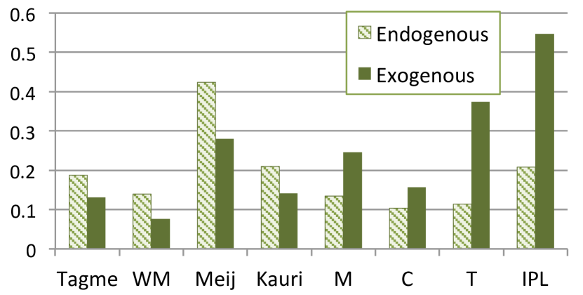
Figure 3: Performance of the methods for different types of trending hashtags.

The performance of the methods in terms of MAP scores is shown in Figure 3. It can be clearly seen that entity linking methods perform well in the endogenous group, but then deteriorate in the exogenous group. The explanation is that for endogenous hashtags, the topical consonance between tweets is very low, thus most of the assessments become just verifying general concepts (such as locations) In this case, topical annotation is trumped by conceptual annotation. However, whenever the hashtag evolves into a meaningful topic, a deeper annotation method will produce a significant improvement, as seen in Figure 3.

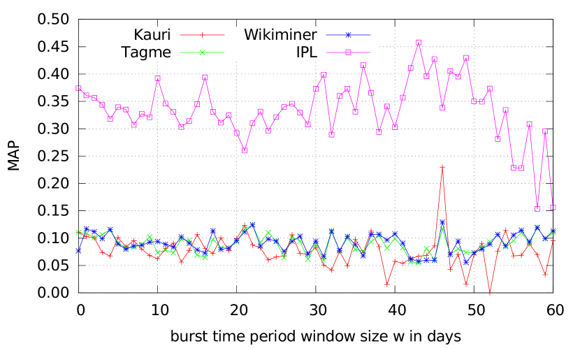
Figure 4: IPL compared to other baselines on different sizes of the burst time window $T$.

Finally, we study the impact of the burst time period on the annotation quality. For this, we expand the window size $w$ (cf. Section 6.1) and examine how different methods perform. The result is depicted in Figure 4. It is obvious that within the window of $2$ months (where the hashtag time series is constructed and a trending time is identified), our method is stable and always outperforms the baselines by a large margin. Even when the trending hashtag has been saturated, hence introduced more noise, our method is still able to identify the prominent entities with high quality.

7 Conclusion and Future Work

In this work, we address the new problem of topically annotating a trending hashtag using Wikipedia entities, which has many important applications in social media analysis. We study Wikipedia temporal resources and find that using efficient time series-based measures can complement content-based methods well in the domain of Twitter. We propose use similarity measures to model both the local mention-based, as well as the global context- and time-based prominence of entities. We propose a novel strategy of topical annotation of texts using and influence maximization approach and design an efficient learning algorithm to automatically unify the similarities without the need of human involvement. The experiments show that our method outperforms significantly the established baselines.

As future work, we aim to improve the efficiency of our entire workflow, such that the annotation can become an end-to-end service. We also aim to improve the context similarity between entities and the topic, for example by using a deeper distributional semantics-based method, instead of language models as in our current work. In addition, we plan to extend the annotation framework to other types of trending topics, by including the type of out-of-knowledge entities. Finally, we are investigating how to apply more advanced influence maximization methods. We believe that influence maximization has a great potential in NLP research, beyond the scope of annotation for microblogging topics.

References

- [Bansal et al., 2015] P. Bansal, R. Bansal, and V. Varma. 2015. Towards deep semantic analysis of hashtags. In ECIR, pages 453–464.
- [Basave et al., 2014] A. E. Cano Basave, G. Rizzo, A. Varga, M. Rowe, M. Stankovic, and A. Dadzie. 2014. Making sense of microposts (#microposts2014) named entity extraction & linking challenge. In 4th Workshop on Making Sense of Microposts.
- [Cassidy et al., 2012] T. Cassidy, H. Ji, L.-A. Ratinov, A. Zubiaga, and H. Huang. 2012. Analysis and enhancement of wikification for microblogs with context expansion. In COLING, pages 441–456.
- [Ciglan and Nørvåg, 2010] M. Ciglan and K. Nørvåg. 2010. WikiPop: personalized event detection system based on Wikipedia page view statistics. In CIKM, pages 1931–1932.
- [Fang and Chang, 2014] Y. Fang and M.-W. Chang. 2014. Entity linking on microblogs with spatial and temporal signals. Trans. of the Assoc. for Comp. Linguistics, 2:259–272.
- [Ferragina and Scaiella, 2012] P. Ferragina and U. Scaiella. 2012. Fast and accurate annotation of short texts with Wikipedia pages. IEEE Softw., 29(1):70–75.
- [Fogaras et al., 2005] D. Fogaras, B. Rácz, K. Csalogány, and T. Sarlós. 2005. Towards scaling fully personalized PageRank: Algorithms, lower bounds, and experiments. Internet Mathematics, 2(3):333–358.
- [Guo et al., 2013] S. Guo, M.-W. Chang, and E. Kıcıman. 2013. To link or not to link? A study on end-to-end tweet entity linking. In NAACL-HLT, pages 1020–1030.
- [Haveliwala, 2002] T. H. Haveliwala. 2002. Topic-sensitive PageRank. In WWW, pages 517–526.
- [Keegan et al., 2011] Brian Keegan, Darren Gergle, and Noshir Contractor. 2011. Hot off the wiki: Dynamics, practices, and structures in wikipedia’s coverage of the tohoku catastrophes. In WikiSym, pages 105–113.
- [Kempe et al., 2003] D. Kempe, J. Kleinberg, and É. Tardos. 2003. Maximizing the spread of influence through a social network. In KDD, pages 137–146.
- [Lappas et al., 2009] T. Lappas, B. Arai, M. Platakis, D. Kotsakos, and D. Gunopulos. 2009. On burstiness-aware search for document sequences. In KDD, pages 477–486.
- [Lehmann et al., 2012] J. Lehmann, B. Gonçalves, J. J. Ramasco, and C. Cattuto. 2012. Dynamical classes of collective attention in Twitter. In WWW, pages 251–260.
- [Liu et al., 2013] X. Liu, Y. Li, H. Wu, M. Zhou, F. Wei, and Y. Lu. 2013. Entity linking for tweets. In ACL, pages 1304–1311.
- [Liu et al., 2014] Q. Liu, B. Xiang, E. Chen, H. Xiong, F. Tang, and J. X. Yu. 2014. Influence maximization over large-scale social networks: A bounded linear approach. In CIKM, pages 171–180.
- [Meij et al., 2012] E. Meij, W. Weerkamp, and M. de Rijke. 2012. Adding semantics to microblog posts. In WSDM, pages 563–572.
- [Milne and Witten, 2008] D. Milne and I. H. Witten. 2008. Learning to link with Wikipedia. In CIKM, pages 509–518.
- [Naaman et al., 2011] M. Naaman, H. Becker, and L. Gravano. 2011. Hip and trendy: Characterizing emerging trends on Twitter. JASIST, 62(5):902–918.
- [Osborne et al., 2012] M. Osborne, S. Petrovic, R. McCreadie, C. Macdonald, and I. Ounis. 2012. Bieber no more: First story detection using Twitter and Wikipedia. In Workshop on Time-aware Information Access.
- [Owoputi et al., 2013] O. Owoputi, B. O’Connor, C. Dyer, K. Gimpel, N. Schneider, and N. A. Smith. 2013. Improved part-of-speech tagging for online conversational text with word clusters. In NAACL-HLT, pages 380–390.
- [Radinsky et al., 2011] K. Radinsky, E. Agichtein, E. Gabrilovich, and S. Markovitch. 2011. A word at a time: Computing word relatedness using temporal semantic analysis. In WWW, pages 337–346.
- [Ratinov et al., 2011] L. Ratinov, D. Roth, D. Downey, and M. Anderson. 2011. Local and Global Algorithms for Disambiguation to Wikipedia. In ACL, pages 1375–1384.
- [Ritter et al., 2011] Alan Ritter, Sam Clark, Oren Etzioni, et al. 2011. Named entity recognition in tweets: an experimental study. In EMNLP, pages 1524–1534.
- [Shen et al., 2013] W. Shen, J. Wang, P. Luo, and M. Wang. 2013. Linking named entities in tweets with knowledge base via user interest modeling. In WSDM, pages 68–76.
- [Tolomei et al., 2013] G. Tolomei, S. Orlando, D. Ceccarelli, and C. Lucchese. 2013. Twitter anticipates bursts of requests for Wikipedia articles. In Workshop on Data-driven User Behavioral Modelling and Mining from Social Media, pages 5–8.
- [Tran and Nguyen, 2014] T. Tran and T. Ngoc Nguyen. 2014. Hedera: Scalable indexing, exploring entities in Wikipedia revision history. In ISWC, pages 297–300.
- [Tran et al., 2014] T. Tran, M. Georgescu, X. Zhu, and N. Kanhabua. 2014. Analysing the duration of trending topics in Twitter using Wikipedia. In Conf. on Web Science, pages 251–252.
- [Tsur and Rappoport, 2012] O. Tsur and A. Rappoport. 2012. What’s in a hashtag?: Content based prediction of the spread of ideas in microblogging communities. In WSDM, pages 643–652.
- [Wang et al., 2011] K. Wang, C. Thrasher, and B.-J. P. Hsu. 2011. Web scale NLP: a case study on URL word breaking. In WWW, pages 357–366.
- [Yang and Leskovec, 2011] J. Yang and J. Leskovec. 2011. Patterns of temporal variation in online media. In WSDM, pages 177–186.