An Online Convex Optimization Approach to Dynamic Network Resource Allocation

Tianyi Chen, , Qing Ling, ,
and Georgios B. Giannakis
Work in this paper was supported by NSF 1509040, 1508993, 1509005, NSF China 61573331, NSF Anhui 1608085QF130, and CAS-XDA06011203.T. Chen and G. B. Giannakis are with the Department of Electrical and Computer Engineering and the Digital Technology Center, University of Minnesota, Minneapolis, MN 55455 USA. Emails: {chen3827, georgios}@umn.edu Q. Ling is with the Department of Automation, University of Science and Technology of China, Hefei, Anhui 230026, China. Email: qingling@mail.ustc.edu.cn
Abstract

Existing approaches to online convex optimization (OCO) make sequential one-slot-ahead decisions, which lead to (possibly adversarial) losses that drive subsequent decision iterates. Their performance is evaluated by the so-called regret that measures the difference of losses between the online solution and the best yet fixed overall solution in hindsight. The present paper deals with online convex optimization involving adversarial loss functions and adversarial constraints, where the constraints are revealed after making decisions, and can be tolerable to instantaneous violations but must be satisfied in the long term. Performance of an online algorithm in this setting is assessed by: i) the difference of its losses relative to the best dynamic solution with one-slot-ahead information of the loss function and the constraint (that is here termed dynamic regret); and, ii) the accumulated amount of constraint violations (that is here termed dynamic fit). In this context, a modified online saddle-point (MOSP) scheme is developed, and proved to simultaneously yield sub-linear dynamic regret and fit, provided that the accumulated variations of per-slot minimizers and constraints are sub-linearly growing with time. MOSP is also applied to the dynamic network resource allocation task, and it is compared with the well-known stochastic dual gradient method. Under various scenarios, numerical experiments demonstrate the performance gain of MOSP relative to the state-of-the-art.

Index Terms:
Constrained optimization, primal-dual method, online convex optimization, network resource allocation.

I Introduction

Online convex optimization (OCO) is an emerging methodology for sequential inference with well documented merits especially when the sequence of convex costs varies in an unknown and possibly adversarial manner [1, 2, 3]. Starting from the seminal papers [1] and [2], most of the early works evaluate OCO algorithms with a static regret, which measures the difference of costs (a.k.a. losses) between the online solution and the overall best static solution in hindsight. If an algorithm incurs static regret that increases sub-linearly with time, then its performance loss averaged over an infinite time horizon goes to zero; see also [3, 4], and references therein.

However, static regret is not a comprehensive performance metric [5]. Take online parameter estimation as an example. When the true parameter varies over time, a static benchmark (time-invariant estimator) itself often performs poorly so that achieving sub-linear static regret is no longer attractive. Recent works [5, 6, 7, 8] extend the analysis of static regret to that of dynamic regret, where the performance of an OCO algorithm is benchmarked by the best dynamic solution with a-priori information on the one-slot-ahead cost function. Sub-linear dynamic regret is proved to be possible, if the dynamic environment changes slow enough for the accumulated variation of either costs or per-slot minimizers to be sub-linearly increasing with respect to the time horizon. When the per-slot costs depend on previous decisions, the so-termed competitive difference can be employed as an alternative of the static regret [9, 10].

The aforementioned works [5, 9, 10, 6, 7, 8] deal with dynamic costs focusing on problems with time-invariant constraints that must be strictly satisfied, but do not allow for instantaneous violations of the constraints. The long-term effect of such instantaneous violations was studied in [11], where an online algorithm with sub-linear static regret and sub-linear accumulated constraint violation was also developed. The regret bounds in [11] have been improved in [12] and [13]. Decentralized optimization with consensus constraints, as a special case of having long-term but time-invariant constraints, has been studied in [14, 15, 16]. Nevertheless, [11, 13, 14, 12, 15, 16] do not deal with OCO under time-varying adversarial constraints.

TABLE I: A summary of related works on discrete time OCO
      Reference       Type of benchmark Long-term constraint Adversarial constraint
[1] Static and dynamic No No
[2, 3, 4] Static No No
[5, 8, 17] Dynamic No No
[6, 7] Dynamic No No
[9, 10] Dynamic No No
[11, 12, 14, 15] Static Yes No
[16] Dynamic Yes No
This work Dynamic Yes Yes

In this context, the present paper considers OCO with time-varying constraints that must be satisfied in the long term. Under this setting, the learner first takes an action without knowing a-priori either the adversarial cost or the time-varying constraint, which are revealed by the nature subsequently. Its performance is evaluated by: i) dynamic regret that is the optimality loss relative to a sequence of instantaneous minimizers with known costs and constraints; and, ii) dynamic fit that accumulates constraint violations incurred by the online learner due to the lack of knowledge about future constraints. We compare the OCO setting here with those of existing works in Table I.

We further introduce a modified online saddle-point (MOSP) method in this novel OCO framework, where the learner deals with time-varying costs as well as time-varying but long-term constraints. We analytically establish that MOSP simultaneously achieves sub-linear dynamic regret and fit, provided that the accumulated variations of both minimizers and constraints grow sub-linearly. This result provides valuable insights for OCO with long-term constraints: When the dynamic environment comprising both costs and constraints does not change on average, the online decisions provided by MOSP are as good as the best dynamic solution over a long time horizon.

To demonstrate the impact of these results, we further apply the proposed MOSP approach to a dynamic network resource allocation task, where online management of resources is sought without knowing future network states. Existing algorithms include first- and second-order methods in the dual domain [18, 19, 20, 21, 22, 23], which are tailored for time-invariant deterministic formulations. To capture the temporal variations of network resources, stochastic formulation of network resource allocation has been extensively pursued since the seminal work of [24]; see also the celebrated stochastic dual gradient method in [25, 26]. These stochastic approximation-based approaches assume that the time-varying costs are i.i.d. or generally samples from a stationary ergodic stochastic process [27, 28, 29]. However, performance of most stochastic schemes is established in an asymptotic sense, considering the ensemble of per slot averages or infinite samples across time. Clearly, stationarity may not hold in practice, especially when the stochastic process involves human participation. Inheriting merits of the OCO framework, the proposed MOSP approach operates in a fully online mode without requiring non-causal information, and further admits finite-sample performance analysis under a sequence of non-stochastic, or even adversarial costs and constraints.

Relative to existing works, the main contributions of the present paper are summarized as follows.

  1. c1)

    We generalize the standard OCO framework with only adversarial costs in [1, 2, 3, 4] to account for both adversarial costs and constraints. Different from the regret analysis in [11, 14, 13, 12, 15], performance here is established relative to the best dynamic benchmark, via metrics that we term dynamic regret and fit.

  2. c2)

    We develop an MOSP algorithm to tackle this novel OCO problem, and analytically establish that MOSP yields simultaneously sub-linear dynamic regret and fit, provided that the accumulated variations of per-slot minimizers and constraints are sub-linearly growing with time.

  3. c3)

    Our novel OCO approach is tailored for dynamic resource allocation tasks, where MOSP is compared with the popular stochastic dual gradient approach. Relative to the latter, MOSP remains operational in a broader practical setting without probabilistic assumptions. Numerical tests demonstrate the gain of MOSP over state-of-the-art alternatives.

Outline. The rest of the paper is organized as follows. The OCO problem with long-term constraints is formulated, and the relevant performance metrics are introduced in Section II. The MOSP algorithm and its performance analysis are presented in Section III. Application of the novel OCO framework and the MOSP algorithm in network resource allocation, as well as corresponding numerical tests, are provided in Section IV. Section V concludes the paper.

Notation. $\mathbb{E}$ denotes expectation, $\mathbb{P}$ stands for probability, $(\cdot)^{\top}$ stands for vector and matrix transposition, and $\|\mathbf{x}\|$ denotes the $\ell_{2}$-norm of a vector $\mathbf{x}$. Inequalities for vectors, e.g., $\mathbf{x}>\mathbf{0}$, are defined entry-wise. The positive projection operator is defined as $[\mathbf{a}]^{+}:=\max\{\mathbf{a},\mathbf{0}\}$, also entry-wise.

II OCO with Long-term Time-varying Constraints

In this section, we introduce the generic OCO formulation with long-term time-varying constraints, along with pertinent metrics to evaluate an OCO algorithm.

II-A Problem formulation

We begin with the classical OCO setting, where constraints are time-invariant and must be strictly satisfied. OCO can be viewed as a repeated game between a learner and nature [3, 1, 2]. Consider that time is discrete and indexed by $t$. Per slot $t$, a learner selects an action $\mathbf{x}_{t}$ from a convex set ${\cal X}\subseteq\mathbb{R}^{I}$, and subsequently nature chooses a (possibly adversarial) loss function $f_{t}(\,\cdot\,):\mathbb{R}^{I}\rightarrow\mathbb{R}$ through which the learner incurs a loss $f_{t}(\mathbf{x}_{t})$. The convex set ${\cal X}$ is a-priori known and fixed over the entire time horizon. Although this standard OCO setting is appealing to various applications such as online regression and classification [1, 2, 3], it does not account for potential variations of (possibly unknown) constraints, and does not deal with constraints that can possibly be satisfied in the long term rather than a slot-by-slot basis. Online optimization with time-varying and long-term constraints is well motivated for applications such as navigation, tracking, and dynamic resource allocation [25, 13, 26, 30]. Taking resource allocation as an example, time-varying long-term constraints are usually imposed to tolerate instantaneous violations when available resources cannot satisfy user requests, and hence allow flexible adaptation of online decisions to temporal variations of resource availability.

To broaden the applicability of OCO to these scenarios, we consider that per slot $t$, a learner selects an action $\mathbf{x}_{t}$ from a known and fixed convex set ${\cal X}\subseteq\mathbb{R}^{I}$, and then nature reveals not only a loss function $f_{t}(\cdot):\mathbb{R}^{I}\rightarrow\mathbb{R}$ but also a time-varying (possibly adversarial) penalty function $\mathbf{g}_{t}(\cdot):\mathbb{R}^{I}\rightarrow\mathbb{R}^{I}$. This function leads to a time-varying constraint $\mathbf{g}_{t}(\mathbf{x})\leq\mathbf{0}$, which is driven by the unknown dynamics in various applications, e.g., on-demand data request arrivals in resource allocation. Different from the known and fixed set ${\cal X}$, the time-varying constraint $\mathbf{g}_{t}(\mathbf{x})\leq\mathbf{0}$ can vary arbitrarily or even adversarially from slot to slot. It is revealed only after the learner makes her/his decision, and hence it is hard to be satisfied in every time slot. Therefore, the goal in this context is to find a sequence of online solutions $\{\mathbf{x}_{t}\in{\cal X}\}$ that minimize the aggregate loss, and ensures that the constraints $\{\mathbf{g}_{t}(\mathbf{x}_{t})\leq\mathbf{0}\}$ are satisfied in the long-term on average. Specifically, we aim to solve the following online optimization problem

$\displaystyle\min_{\{\mathbf{x}_{t}\in{\cal X},\forall t\}}~{}$ $\displaystyle\sum_{t=1}^{T}f_{t}(\mathbf{x}_{t})$ (1a)
s. t. $\displaystyle\sum_{t=1}^{T}\mathbf{g}_{t}(\mathbf{x}_{t})\leq\mathbf{0}$ (1b)

where $T$ is the time horizon, $\mathbf{x}_{t}\in\mathbb{R}^{I}$ is the decision variable, $f_{t}$ is the cost function, $\mathbf{g}_{t}:=[g_{t}^{1},\ldots,g_{t}^{I}]^{\top}$ denotes the constraint function with $i$th entry $g_{t}^{i}:\mathbb{R}^{I}\rightarrow\mathbb{R}$, and ${\cal X}\in\mathbb{R}^{I}$ is a convex set. The formulation (1) extends the standard OCO framework to accommodate adversarial time-varying constraints that must be satisfied in the long term. Complemented by algorithm development and performance analysis to be carried in the following sections, the main contribution of the present paper is incorporation of long-term and time-varying constraints to markedly broaden the scope of OCO.

II-B Performance and feasibility metrics

Regarding performance of online decisions $\{\mathbf{x}_{t}\}_{t=1}^{T}$, static regret is adopted as a metric by standard OCO schemes, under time-invariant and strictly satisfied constraints. The static regret measures the difference between the online loss of an OCO algorithm and that of the best fixed solution in hindsight [1, 2, 3]. Extending the definition of static regret over $T$ slots to accommodate time-varying constraints, it can be written as (see also [13])

$\displaystyle{\rm Reg}_{T}^{\rm s}:=\sum_{t=1}^{T}f_{t}(\mathbf{x}_{t})-\sum_{t=1}^{T}f_{t}(\mathbf{x}^{*})$ (2)

where the best static solution $\mathbf{x}^{*}$ is obtained as

$$\mathbf{x}^{*}\in\arg\min_{\mathbf{x}\in{\cal X}}\,\sum_{t=1}^{T}f_{t}(\mathbf{x})~{}~{}\text{s. t.}~{}\mathbf{g}_{t}(\mathbf{x})\leq\mathbf{0},\;\forall t.$$ (3)

A desirable OCO algorithm in this case is the one yielding a sub-linear regret [11, 12], meaning ${\rm Reg}_{T}^{\rm s}=\mathbf{o}(T)$. Consequently, $\lim_{T\rightarrow\infty}{{\rm Reg}_{T}^{\rm s}}/{T}=0$ implies that the algorithm is “on average” no-regret, or in other words, not worse asymptotically than the best fixed solution $\mathbf{x}^{*}$. Though widely used in various OCO applications, the aforementioned static regret metric relies on a rather coarse benchmark, which may be less useful especially in dynamic settings. For instance, [5, Example 2] shows that the gap between the best static and the best dynamic benchmark can be as large as ${\cal O}(T)$. Furthermore, since the time-varying constraint $\mathbf{g}_{t}(\mathbf{x}_{t})\leq\mathbf{0}$ is not observed before making a decision $\mathbf{x}_{t}$, its feasibility can not be checked instantaneously.

In response to the quest for improved benchmarks in this dynamic setup, two metrics are considered here: dynamic regret and dynamic fit. The notion of dynamic regret (also termed tracking regret or adaptive regret) has been recently introduced in [5, 6, 7, 8] to offer a competitive performance measure of OCO algorithms under time-invariant constraints. We adopt it in the setting of (1) by incorporating time-varying constraints

$\displaystyle{\rm Reg}^{\rm d}_{T}:=\sum_{t=1}^{T}f_{t}(\mathbf{x}_{t})-\sum_{t=1}^{T}f_{t}(\mathbf{x}_{t}^{*})$ (4)

where the benchmark is now formed via a sequence of best dynamic solutions $\{\mathbf{x}_{t}^{*}\}$ for the instantaneous cost minimization problem subject to the instantaneous constraint, namely

$$\mathbf{x}_{t}^{*}\in\arg\min_{\mathbf{x}\in{\cal X}}\;f_{t}(\mathbf{x})~{}~{}~{}\text{s. t.}~{}\mathbf{g}_{t}(\mathbf{x})\leq\mathbf{0}.$$ (5)

Clearly, the dynamic regret is always larger than the static regret in (2), i.e., ${\rm Reg}^{\rm s}_{T}\leq{\rm Reg}^{\rm d}_{T}$, because $\sum_{t=1}^{T}f_{t}(\mathbf{x}^{*})$ is always no smaller than $\sum_{t=1}^{T}f_{t}(\mathbf{x}^{*}_{t})$ according to the definitions of $\mathbf{x}^{*}$ and $\mathbf{x}^{*}_{t}$. Hence, a sub-linear dynamic regret implies a sub-linear static regret, but not vice versa.

To ensure feasibility of online decisions, the notion of dynamic fit is introduced to measure the accumulated violation of constraints; under time-invariant long-term constraints [11, 14, 12] or under time-varying constraints [13]. It is defined as

$\displaystyle{\rm Fit}^{\rm d}_{T}:=\left\|\left[\sum_{t=1}^{T}\mathbf{g}_{t}(\mathbf{x}_{t})\right]^{+}\right\|.$ (6)

Observe that the dynamic fit is zero if the accumulated violation $\sum_{t=1}^{T}\mathbf{g}_{t}(\mathbf{x}_{t})$ is entry-wise less than zero. However, enforcing $\sum_{t=1}^{T}\mathbf{g}_{t}(\mathbf{x}_{t})\leq\mathbf{0}$ is different from restricting $\mathbf{x}_{t}$ to meet $\mathbf{g}_{t}(\mathbf{x}_{t})\leq\mathbf{0}$ in each and every slot. While the latter readily implies the former, the long-term (aggregate) constraint allows adaptation of online decisions to the environment dynamics; as a result, it is tolerable to have $\mathbf{g}_{t}(\mathbf{x}_{t})\geq\mathbf{0}$ and $\mathbf{g}_{t+1}(\mathbf{x}_{t+1})\leq\mathbf{0}$.

An ideal algorithm in this broader OCO framework is the one that achieves both sub-linear dynamic regret and sub-linear dynamic fit. A sub-linear dynamic regret implies “no-regret” relative to the clairvoyant dynamic solution on the long-term average; i.e., $\lim_{T\rightarrow\infty}{{\rm Reg}_{T}^{\rm d}}/{T}=0$; and a sub-linear dynamic fit indicates that the online strategy is also feasible on average; i.e., $\lim_{T\rightarrow\infty}{{\rm Fit}_{T}^{\rm d}}/{T}=0$. Unfortunately, the sub-linear dynamic regret is not achievable in general, even under the special case of (1) where the time-varying constraint is absent [5]. For this reason, we aim at designing and analyzing an online strategy that generates a sequence $\{\mathbf{x}_{t}\}_{t=1}^{T}$ ensuring sub-linear dynamic regret and fit, under mild conditions that must be satisfied by the cost and constraint variations.

III Modified Online saddle-point (MOSP) Method

In this section, a modified online saddle-point method is developed to solve (1), and its performance and feasibility are analyzed using the dynamic regret and fit metrics.

III-A Algorithm development

Consider now the per-slot problem (5), which contains the current objective $f_{t}(\mathbf{x})$, the current constraint $\mathbf{g}_{t}(\mathbf{x})\leq\mathbf{0}$, and a time-invariant constraint set ${\cal X}$. With $\bm{\lambda}\in\mathbb{R}^{N}_{+}$ denoting the Lagrange multiplier associated with the time-varying constraint, the online (partial) Lagrangian of (5) can be expressed as

$\displaystyle{\cal L}_{t}(\mathbf{x},\bm{\lambda}):=f_{t}(\mathbf{x})+\bm{\lambda}^{\top}\mathbf{g}_{t}(\mathbf{x})$ (7)

where $\mathbf{x}\in{\cal X}$ remains implicit. For the online Lagrangian (7), we introduce a modified online saddle point (MOSP) approach, which takes a modified descent step in the primal domain, and a dual ascent step at each time slot $t$. Specifically, given the previous primal iterate $\mathbf{x}_{t-1}$ and the current dual iterate $\bm{\lambda}_{t}$ at each slot $t$, the current decision $\mathbf{x}_{t}$ is the minimizer of the following optimization problem

$$\min_{\mathbf{x}\in{\cal X}}\,\nabla^{\top}f_{t-1}(\mathbf{x}_{t-1})\!\left(\mathbf{x}-\mathbf{x}_{t-1}\right)+\bm{\lambda}_{t}^{\top}\mathbf{g}_{t-1}(\mathbf{x})+\frac{\|\mathbf{x}-\mathbf{x}_{t-1}\|^{2}}{2\alpha}$$ (8)

where $\alpha$ is a positive stepsize, and $\nabla f_{t-1}(\mathbf{x}_{t-1})$ is the gradient111One can replace the gradient by one of the sub-gradients when $f_{t}(\mathbf{x})$ is non-differentiable. The performance analysis still holds true for this case. of primal objective $f_{t-1}(\mathbf{x})$ at $\mathbf{x}=\mathbf{x}_{t-1}$. After the current decision $\mathbf{x}_{t}$ is made, $f_{t}(\mathbf{x})$ and $\mathbf{g}_{t}(\mathbf{x})$ are observed, and the dual update takes the form

$$\bm{\lambda}_{t+1}=\big{[}\bm{\lambda}_{t}+\mu\nabla_{\bm{\lambda}}{\cal L}_{t}(\mathbf{x}_{t},\bm{\lambda}_{t})\big{]}^{+}=\big{[}\bm{\lambda}_{t}+\mu\mathbf{g}_{t}(\mathbf{x}_{t})\big{]}^{+}$$ (9)

where $\mu$ is also a positive stepsize, and $\nabla_{\bm{\lambda}}{\cal L}_{t}(\mathbf{x}_{t},\bm{\lambda}_{t})=\mathbf{g}_{t}(\mathbf{x}_{t})$ is the gradient of online Lagrangian (7) with respect to (w.r.t.) $\bm{\lambda}$ at $\bm{\lambda}=\bm{\lambda}_{t}$.

Remark 1.

The primal gradient step of the classical saddle-point approach in [14, 11, 13] is tantamount to minimizing a first-order approximation of ${\cal L}_{t-1}(\mathbf{x},\bm{\lambda}_{t})$ at $\mathbf{x}=\mathbf{x}_{t-1}$ plus a proximal term $\|\mathbf{x}-\mathbf{x}_{t-1}\|^{2}/(2\alpha)$. We call the primal-dual recursion (8) and (9) as a modified online saddle-point approach, since the primal update (8) is not an exact gradient step when the constraint $\mathbf{g}_{t}(\mathbf{x})$ is nonlinear w.r.t. $\mathbf{x}$. However, when $\mathbf{g}_{t}(\mathbf{x})$ is linear, (8) and (9) reduce to the approach in [14, 11, 13]. Similar to the primal update of OCO with long-term but time-invariant constraints in [12], the minimization in (8) penalizes the exact constraint violation $\mathbf{g}_{t}(\mathbf{x})$ instead of its first-order approximation, which improves control of constraint violations and facilitates performance analysis of MOSP.

Algorithm 1 Modified online saddle-point (MOSP) method
1:Initialize: primal iterate $\mathbf{x}_{0}$, dual iterate $\bm{\lambda}_{1}$, and proper stepsizes $\alpha$ and $\mu$.
2:for $t=1,2\dots$ do
3:     Update primal variable $\mathbf{x}_{t}$ by solving (8).
4:     Observe the current cost $f_{t}(\mathbf{x})$ and constraint $\mathbf{g}_{t}(\mathbf{x})$.
5:     Update the dual variable $\bm{\lambda}_{t+1}$ via (9).
6:end for

III-B Performance analysis

We proceed to show that for MOSP, the dynamic regret in (4) and the dynamic fit in (6) are both sub-linearly increasing if the variations of the per-slot minimizers and the constraints are small enough. Before formally stating this result, we assume that the following conditions are satisfied.

Assumption 1.

For every $t$, the cost function $f_{t}(\mathbf{x})$ and the time-varying constraint $\mathbf{g}_{t}(\mathbf{x})$ in (1) are convex.

Assumption 2.

For every $t$, $f_{t}(\mathbf{x})$ has bounded gradient on ${\cal X}$; i.e., $\|\nabla f_{t}(\mathbf{x})\|\leq G,\;\forall\mathbf{x}\in{\cal X}$; and $\mathbf{g}_{t}(\mathbf{x})$ is bounded on ${\cal X}$; i.e., $\|\mathbf{g}_{t}(\mathbf{x})\|\leq M,\;\forall\mathbf{x}\in{\cal X}$.

Assumption 3.

The radius of the convex feasible set ${\cal X}$ is bounded; i.e., $\|\mathbf{x}-\mathbf{y}\|\leq R,\;\forall\mathbf{x},\mathbf{y}\in{\cal X}$.

Assumption 4.

There exists a constant $\epsilon>0$, and an interior point $\tilde{\mathbf{x}}\in{\cal X}$ such that $\mathbf{g}_{t}(\tilde{\mathbf{x}})\leq-\epsilon\mathbf{1},\;\forall t$.

Assumption 1 is necessary for regret analysis in the OCO setting. Assumption 2 bounds primal and dual gradients per slot, which is also typical in OCO [3, 12, 14, 6]. Assumption 3 restricts the action set to be bounded. Assumption 4 is Slater’s condition, which guarantees the existence of a bounded Lagrange multiplier [31].

Under these assumptions, we are on track to first provide an upper bound for the dynamic fit.

Theorem 1.

Define the maximum variation of consecutive constraints as

$$\bar{V}(\mathbf{g})\!:=\!\max_{t}V(\mathbf{g}_{t}),{\rm~{}with~{}}V(\mathbf{g}_{t})\!:=\!\max_{\mathbf{x}\in{\cal X}}\,\left\|\left[\mathbf{g}_{t+1}(\mathbf{x})\!-\!\mathbf{g}_{t}(\mathbf{x})\right]^{+}\right\|$$ (10)

and assume the slack constant $\epsilon$ in Assumption 4 to be larger than the maximum variation222This equivalently requires $\epsilon:=\min_{i,t}\max_{\mathbf{x}\in{\cal X}}[-g^{i}_{t}(\mathbf{x})]^{+}>\max_{\mathbf{x}\in{\cal X}}$ $\big{\|}\big{[}\mathbf{g}_{t+1}(\mathbf{x})-\mathbf{g}_{t}(\mathbf{x})\big{]}^{+}\big{\|}$, which is valid when the region defined by $\mathbf{g}_{t}(\mathbf{x})\leq\mathbf{0}$ is large enough, or, the trajectory of $\mathbf{g}_{t}(\mathbf{x})$ is smooth enough across time.; i.e., $\epsilon>\bar{V}(\mathbf{g})$. Then under Assumptions 1-4 and the dual variable initialization $\bm{\lambda}_{1}=\mathbf{0}$, the dual iterate for the MOSP recursion (8)-(9) is bounded by

$$\|\bm{\lambda}_{t}\|\leq\|\bar{\bm{\lambda}}\|:=\mu M+\frac{2GR+{R^{2}}/(2\alpha)+(\mu M^{2})/{2}}{\epsilon-\bar{V}(\mathbf{g})},\;\forall t$$ (11)

and the dynamic fit in (6) is upper-bounded by

$\displaystyle{\rm Fit}^{\rm d}_{T}\leq\frac{\|\bm{\lambda}_{T+1}\|}{\mu}\leq\frac{\|\bar{\bm{\lambda}}\|}{\mu}=M+\frac{2GR/\mu\!+\!{R^{2}}/(2\alpha\mu)\!+\!M^{2}/2}{\epsilon-\bar{V}(\mathbf{g})}$ (12)

where $G$, $M$, $R$, and $\epsilon$ are as in Assumptions 2-4.

Proof.

See Appendix -A. ∎

Theorem 1 asserts that under a mild condition on the time-varying constraints, $\|\bm{\lambda}_{t}\|$ is uniformly upper-bounded, and more importantly, its scaled version ${\|\bm{\lambda}_{T+1}\|}/{\mu}$ upper bounds the dynamic fit. Observe that with a fixed primal stepsize $\alpha$, ${\rm Fit}^{\rm d}_{T}$ is in the order of ${\cal O}(1/\mu)$, thus a larger dual stepsize essentially enables a better satisfaction of long-term constraints. In addition, a smaller $\bar{V}(\mathbf{g})$ leads to a smaller dynamic fit, which also makes sense intuitively.

In the next theorem, we further bound the dynamic regret.

Theorem 2.

Under Assumptions 1-4 and the dual variable initialization $\bm{\lambda}_{1}=\mathbf{0}$, the MOSP recursion (8)-(9) yields a dynamic regret

$\displaystyle{\rm Reg}^{\rm d}_{T}\!\leq\!\frac{RV(\{\mathbf{x}_{t}^{*}\}_{t=1}^{T})}{\alpha}$ $\displaystyle+\!\|\bar{\bm{\lambda}}\|V(\{\mathbf{g}_{t}\}_{t=1}^{T})\!+\!\frac{R^{2}}{2\alpha}$
$\displaystyle+\frac{\alpha G^{2}T}{2}+\!\frac{\mu M^{2}(T+1)}{2}$ (13)

where $V(\{\mathbf{x}_{t}^{*}\}_{t=1}^{T})$ is the accumulated variation of the per-slot minimizers $\mathbf{x}^{*}_{t}$ defined as

$\displaystyle V(\{\mathbf{x}_{t}^{*}\}_{t=1}^{T}):=\sum_{t=1}^{T}\|\mathbf{x}^{*}_{t}-\mathbf{x}^{*}_{t-1}\|$ (14)

and $V(\{\mathbf{g}_{t}\}_{t=1}^{T})$ is the accumulated variation of consecutive constraints

$\displaystyle\!\!\!V(\{\mathbf{g}_{t}\}_{t=1}^{T})\!:=\!\sum_{t=1}^{T}\!V(\mathbf{g}_{t})\!=\!\sum_{t=1}^{T}\max_{\mathbf{x}\in{\cal X}}\!\left\|\left[\mathbf{g}_{t+1}(\mathbf{x})\!-\!\mathbf{g}_{t}(\mathbf{x})\right]^{+}\right\|\!.\!$ (15)
Proof.

See Appendix -B. ∎

Theorem 2 asserts that MOSP’s dynamic regret is upper-bounded by a constant depending on the accumulated variations of per-slot minimizers and time-varying constraints as well as the primal and dual stepsizes. While the dynamic regret in the current form (2) is hard to grasp, the next corollary shall demonstrate that ${\rm Reg}^{\rm d}_{T}$ can be very small.

Based on Theorems 1-2, we are ready to establish that under the mild conditions for the accumulated variation of constraints and minimizers, the dynamic regret and fit are sub-linearly increasing with $T$.

Corollary 1.

Under Assumptions 1-4 and the dual variable initialization $\bm{\lambda}_{1}=\mathbf{0}$, if the primal and dual stepsizes are chosen such that $\alpha=\mu={\cal O}(T^{-\frac{1}{3}})$, then the dynamic fit is upper-bounded by

$$\!{\rm Fit}^{\rm d}_{T}\!=\!{\cal O}\!\left(\!M\!+\!\frac{2GRT^{1/3}\!+\!{R^{2}T^{2/3}}/2\!+\!M^{2}/2}{\epsilon-\bar{V}(\mathbf{g})}\!\right)\!\!=\!{\cal O}(T^{\frac{2}{3}}).\!\!\!\!$$ (16)

In addition, if the temporal variations of optimal arguments and constraints satisfy $V(\{\mathbf{x}_{t}^{*}\}_{t=1}^{T})=\mathbf{o}(T^{\frac{2}{3}})$ and $V(\{\mathbf{g}_{t}\}_{t=1}^{T})=\mathbf{o}(T^{\frac{2}{3}})$, then the dynamic regret is sub-linearly increasing, i.e.,

$${\rm Reg}^{\rm d}_{T}=\mathbf{o}(T).$$ (17)
Proof.

Plugging $\alpha=\mu={\cal O}(T^{-\frac{1}{3}})$ into (12), the bound in (16) readily follows. Likewise, we have from (2) that

$\displaystyle{\rm Reg}^{\rm d}_{T}={\cal O}\Big{(}RV(\{\mathbf{x}_{t}^{*}\}_{t=1}^{T})T^{\frac{1}{3}}$ $\displaystyle+\!\|\bar{\bm{\lambda}}\|V(\{\mathbf{g}_{t}\}_{t=1}^{T})\!+\!\frac{R^{2}T^{\frac{1}{3}}}{2}$
$\displaystyle+\frac{G^{2}T^{\frac{2}{3}}}{2}+\!\frac{M^{2}T^{\frac{2}{3}}}{2}\Big{)}.$ (18)

Considering the upper bound on the dual iterates in (11), it follows that $\|\bar{\bm{\lambda}}\|={\cal O}(\mu+1/\alpha)={\cal O}(T^{\frac{1}{3}})$, which implies that

$${\rm Reg}^{\rm d}_{T}\!=\!{\cal O}\left(\max\left\{V(\{\mathbf{x}_{t}^{*}\}_{t=1}^{T})T^{\frac{1}{3}},\,V(\{\mathbf{g}_{t}\}_{t=1}^{T})T^{\frac{1}{3}},\,T^{\frac{2}{3}}\right\}\right).\!\!$$ (19)

Therefore, we deduce that ${\rm Reg}^{\rm d}_{T}=\mathbf{o}(T)$, if $V(\{\mathbf{x}_{t}^{*}\}_{t=1}^{T})=\mathbf{o}(T^{\frac{2}{3}})$ and $V(\{\mathbf{g}_{t}\}_{t=1}^{T})=\mathbf{o}(T^{\frac{2}{3}})$. ∎

Observe that the sub-linear regret and fit in Corollary 1 are achieved under a slightly “strict” condition that $V(\{\mathbf{x}_{t}^{*}\}_{t=1}^{T})=\mathbf{o}(T^{\frac{2}{3}})$ and $V(\{\mathbf{g}_{t}\}_{t=1}^{T})=\mathbf{o}(T^{\frac{2}{3}})$. The next corollary shows that this condition can be further relaxed if a-priori knowledge of the time-varying environment is available.

Corollary 2.

Consider Assumptions 1-4 are satisfied, and the dual variable is initialized as $\bm{\lambda}_{1}=\mathbf{0}$. If there exists a constant $\beta\in[0,1)$ such that the temporal variations satisfy $V(\{\mathbf{x}_{t}^{*}\}_{t=1}^{T})=\mathbf{o}(T^{\beta})$ and $V(\{\mathbf{g}_{t}\}_{t=1}^{T})=\mathbf{o}(T^{\beta})$, then choosing the primal and dual stepsizes as $\alpha=\mu={\cal O}(T^{\frac{\beta-1}{2}})$ leads to the dynamic fit

$${\rm Fit}^{\rm d}_{T}\!=\!{\cal O}\!\left(T^{\frac{1-\beta}{2}}\!+T^{1-\beta}\right)\!=\!{\cal O}(T^{1-\beta})=\mathbf{o}(T)$$ (20)

and the corresponding dynamic regret

$${\rm Reg}^{\rm d}_{T}=\!{\cal O}\!\left(T^{\frac{\beta+1}{2}}\!+\!T^{\frac{1-\beta}{2}}\!+\!T^{\frac{\beta+1}{2}}\right)\!\!=\!{\cal O}(T^{\frac{\beta+1}{2}})=\mathbf{o}(T).$$ (21)

Corollary 2 provides valuable insights for choosing optimal stepsizes in non-stationary settings. Specifically, adjusting stepsizes to match the variability of the dynamic environment is the key to achieving the optimal performance in terms of dynamic regret and fit. Intuitively, when the variation of the environment is fast (a larger $\beta$), slowly decaying stepsizes (thus larger stepsizes) can better track the potential changes.

Remark 2.

Theorems 1 and 2 are in the spirit of the recent work [5, 8, 17], where the regret bounds are established with respect to a dynamic benchmark in either deterministic or stochastic settings. However, [5, 8, 17] do not account for long-term and time-varying constraints, while the dynamic regret analysis is generalized here to the setting with long-term constraints. Interesting though, sub-linear dynamic regret and fit can be achieved when the dynamic environment consisting of the per-slot minimizer and the time-varying constraint does not vary on average, that is, $V(\{\mathbf{x}_{t}^{*}\}_{t=1}^{T})$ and $V(\{\mathbf{g}_{t}\}_{t=1}^{T})$ are sub-linearly increasing over $T$.

III-C Beyond dynamic regret

Although the dynamic benchmark in (4) is more competitive than the static one in (2), it is worth noting that the sequence of the per-slot minimizer $\mathbf{x}_{t}^{*}$ in (5) is not the optimal solution to problem (1). Defining the sequence of optimal solutions to (1) as $\{\mathbf{x}_{t}^{\rm off}\}_{t=1}^{T}$, it is instructive to see that computing each minimizer $\mathbf{x}_{t}^{*}$ in (5) only requires one-slot-ahead information (namely, $f_{t}(\mathbf{x})$ and $g_{t}(\mathbf{x})$), while computing each $\mathbf{x}_{t}^{\rm off}$ within $\{\mathbf{x}_{t}^{\rm off}\}_{t=1}^{T}$ requires information over the entire time horizon (that is, $\{f_{t}(\mathbf{x})\}_{t=1}^{T}$ and $\{g_{t}(\mathbf{x})\}_{t=1}^{T}$). For this reason, we use the subscript “off” in $\{\mathbf{x}_{t}^{\rm off}\}_{t=1}^{T}$ to emphasize that this solution comes from offline computation with information over $T$ slots. Note that for the cases without long-term constraints [5, 6, 7, 8], the sequence of offline solutions $\{\mathbf{x}_{t}^{\rm off}\}_{t=1}^{T}$ coincides with the sequence of per-slot minimizers $\{\mathbf{x}_{t}^{*}\}_{t=1}^{T}$.

Regarding feasibility, $\{\mathbf{x}_{t}^{\rm off}\}_{t=1}^{T}$ exactly satisfies the long-term constraint (1b), while the solution of MOSP satisfies (1b) on average under mild conditions (cf. Corollary 1). For optimality, the cost of the online decisions $\{\mathbf{x}_{t}\}_{t=1}^{T}$ attained by MOSP is further benchmarked by the offline solutions $\{\mathbf{x}_{t}^{\rm off}\}_{t=1}^{T}$. To this end, define MOSP’s optimality gap as

$${\rm OptGap}^{\rm off}_{T}:=\sum_{t=1}^{T}f_{t}(\mathbf{x}_{t})-\sum_{t=1}^{T}f_{t}(\mathbf{x}_{t}^{\rm off}).$$ (22a)
Intuitively, if $\{\mathbf{x}_{t}^{\rm off}\}_{t=1}^{T}$ are close to $\{\mathbf{x}_{t}^{*}\}_{t=1}^{T}$, the dynamic regret ${\rm Reg}^{\rm d}_{T}$ is able to provide an accurate performance measure in the sense of ${\rm OptGap}^{\rm off}_{T}$. Specifically, one can decompose the optimality gap as
$${\rm OptGap}^{\rm off}_{T}\!=\!\underbrace{\sum_{t=1}^{T}f_{t}(\mathbf{x}_{t})\!-\!\sum_{t=1}^{T}f_{t}(\mathbf{x}_{t}^{*})}_{{\cal U}_{1}}+\underbrace{\sum_{t=1}^{T}f_{t}(\mathbf{x}_{t}^{*})\!-\!\sum_{t=1}^{T}f_{t}(\mathbf{x}_{t}^{\rm off})}_{{\cal U}_{2}}$$ (22b)

where ${\cal U}_{1}$ corresponds to the dynamic regret ${\rm Reg}^{\rm d}_{T}$ in (4) capturing the regret relative to the sequence of per-slot minimizers with one-slot-ahead information, and ${\cal U}_{2}$ is the difference between the performance of per-slot minimizers and the offline optimal solutions. Although the second term appears difficult to quantify, we will show next that ${\cal U}_{2}$ is driven by the accumulated variation of the dual functions associated with the instantaneous problems (5).

To this end, consider the dual function of the instantaneous primal problem (5), which can be expressed by minimizing the online Lagrangian in (7) at time $t$, namely [31]

$\displaystyle{\cal D}_{t}(\bm{\lambda}):=\min_{\mathbf{x}\in{\cal X}}\;{\cal L}_{t}(\mathbf{x},\bm{\lambda})=\min_{\mathbf{x}\in{\cal X}}\;f_{t}(\mathbf{x})+\bm{\lambda}^{\top}\mathbf{g}_{t}(\mathbf{x}).$ (23)

Likewise, the dual function of (1) over the entire horizon is

$\displaystyle{\cal D}(\bm{\lambda})$ $\displaystyle:=\min_{\{\mathbf{x}_{t}\in{\cal X},\forall t\}}\;\sum_{t=1}^{T}{\cal L}_{t}(\mathbf{x}_{t},\bm{\lambda})$
$\displaystyle\stackrel{{\scriptstyle(a)}}{{=}}\sum_{t=1}^{T}\min_{\mathbf{x}_{t}\in{\cal X}}{\cal L}_{t}(\mathbf{x}_{t},\bm{\lambda})\stackrel{{\scriptstyle(b)}}{{=}}\sum_{t=1}^{T}{\cal D}_{t}(\bm{\lambda})$ (24)

where equality (a) holds since the minimization is separable across the summand at time $t$, and equality (b) is due to the definition of the per-slot dual function in (23). As the primal problems (1) and (5) are both convex, Slater’s condition in Assumption 4 implies that strong duality holds. Accordingly, ${\cal U}_{2}$ in (22b) can be written as

$$\sum_{t=1}^{T}f_{t}(\mathbf{x}_{t}^{*})-\sum_{t=1}^{T}f_{t}(\mathbf{x}_{t}^{\rm off})=\sum_{t=1}^{T}\;\max_{\bm{\lambda}\geq\mathbf{0}}{\cal D}_{t}(\bm{\lambda})-\max_{\bm{\lambda}\geq\mathbf{0}}\sum_{t=1}^{T}{\cal D}_{t}(\bm{\lambda})$$ (25)

which is the difference between the dual objective of the static best solution, i.e., $\bm{\lambda}^{*}\!\in\!\arg\max_{\bm{\lambda}\geq\mathbf{0}}\!\sum_{t=1}^{T}\!{\cal D}_{t}(\bm{\lambda})$, and that of the per-slot best solution for (23), i.e., $\bm{\lambda}_{t}^{*}\!\in\!\arg\max_{\bm{\lambda}\geq\mathbf{0}}\!{\cal D}_{t}(\bm{\lambda})$. Leveraging this special property of the dual problem, we next establish that ${\cal U}_{2}$ can be bounded by the variation of the dual function, thus providing an estimate of the optimality gap (22a).

Proposition 1.

Define the variation of the dual function (23) from time $t$ to $t+1$ as

$$V({\cal D}_{t}):=\max_{\bm{\lambda}\geq\mathbf{0}}\|{\cal D}_{t+1}(\bm{\lambda})-{\cal D}_{t}(\bm{\lambda})\|$$ (26)

and the total variation over the time horizon $T$ as $V(\{{\cal D}_{t}\}_{t=1}^{T}):=\sum_{t=1}^{T}V({\cal D}_{t})$. Then the cost difference between the best offline solution and the best dynamic solution satisfies

$$\sum_{t=1}^{T}f_{t}(\mathbf{x}_{t}^{*})-\sum_{t=1}^{T}f_{t}(\mathbf{x}_{t}^{\rm off})\leq 2TV(\{{\cal D}_{t}\}_{t=1}^{T})$$ (27)

where $\mathbf{x}_{t}^{*}$ is the minimizer of the instantaneous problem (5), and $\mathbf{x}_{t}^{\rm off}$ solves (1) with all future information available. Combined with (22b), it readily follows that

$${\rm OptGap}^{\rm off}_{T}\leq{\rm Reg}^{\rm d}_{T}+2TV(\{{\cal D}_{t}\}_{t=1}^{T})$$ (28)

where ${\rm Reg}^{\rm d}_{T}$ is defined in (4), and ${\rm OptGap}^{\rm off}_{T}$ in (22).

Proof.

Instead of going to the primal domain, we upper bound ${\cal U}_{2}$ via the dual representation in (25). Letting $\tilde{t}$ denote any slot in ${\cal T}:=\{1,\ldots,T\}$, we have

$\displaystyle\sum_{t\in{\cal T}}\;\max_{\bm{\lambda}\geq\mathbf{0}}{\cal D}_{t}(\bm{\lambda})-\max_{\bm{\lambda}\geq\mathbf{0}}\sum_{t\in{\cal T}}{\cal D}_{t}(\bm{\lambda})$ (29)
$\displaystyle\leq$ $\displaystyle\sum_{t\in{\cal T}}\left({\cal D}_{t}(\bm{\lambda}_{t}^{*})-{\cal D}_{t}(\bm{\lambda}_{\tilde{t}}^{*})\right)\leq T\max_{t\in{\cal T}}\left\{{\cal D}_{t}(\bm{\lambda}_{t}^{*})\!-\!{\cal D}_{t}(\bm{\lambda}_{\tilde{t}}^{*})\right\}.$

The first inequality comes from the definition $\bm{\lambda}_{t}^{*}\!\in\!\arg\max_{\bm{\lambda}\geq\mathbf{0}}\!{\cal D}_{t}(\bm{\lambda})$. Note that if $\max_{t\in{\cal T}}\{{\cal D}_{t}(\bm{\lambda}_{t}^{*})\!-\!{\cal D}_{t}(\bm{\lambda}_{\tilde{t}}^{*})\}\leq 2V(\{{\cal D}_{t}\}_{t=1}^{T})$, the proposition readily follows from (29). We will prove this inequality by contradiction. Assume there exists a slot $t_{0}\in{\cal T}$ such that ${\cal D}_{t_{0}}(\bm{\lambda}_{t_{0}}^{*})-{\cal D}_{t_{0}}(\bm{\lambda}_{\tilde{t}}^{*})>2V(\{{\cal D}_{t}\}_{t=1}^{T})$, which implies that

$\displaystyle{\cal D}_{\tilde{t}}(\bm{\lambda}_{\tilde{t}}^{*})$ $\displaystyle\stackrel{{\scriptstyle(a)}}{{\leq}}{\cal D}_{t_{0}}(\bm{\lambda}_{\tilde{t}}^{*})+V(\{{\cal D}_{t}\}_{t=1}^{T})\stackrel{{\scriptstyle(b)}}{{<}}{\cal D}_{t_{0}}(\bm{\lambda}_{t_{0}}^{*})-V(\{{\cal D}_{t}\}_{t=1}^{T})$
$\displaystyle\stackrel{{\scriptstyle(c)}}{{\leq}}{\cal D}_{\tilde{t}}(\bm{\lambda}_{t_{0}}^{*}),\;\forall\;\tilde{t}\in{\cal T}$ (30)

where inequalities (a) and (c) come from the fact that $V(\{{\cal D}_{t}\}_{t=1}^{T})$ is the accumulated variation over $T$ slots, and hence $\max_{t_{1},t_{2}\in{\cal T}}\|{\cal D}_{t_{1}}(\bm{\lambda})-{\cal D}_{t_{2}}(\bm{\lambda})\|\leq V(\{{\cal D}_{t}\}_{t=1}^{T})$, while (b) is due to the hypothesis above. Note that ${\cal D}_{\tilde{t}}(\bm{\lambda}_{\tilde{t}}^{*})<{\cal D}_{\tilde{t}}(\bm{\lambda}_{t_{0}}^{*})$ in (III-C) contradicts the fact that $\bm{\lambda}_{\tilde{t}}^{*}$ is the maximizer of ${\cal D}_{\tilde{t}}(\bm{\lambda})$. Therefore, we have ${\cal D}_{t}(\bm{\lambda}_{\tilde{t}}^{*})-{\cal D}_{t}(\bm{\lambda}_{t}^{*})\!\leq\!2V(\{{\cal D}_{t}\}_{t=1}^{T})$, which completes the proof. ∎

The following remark provides an approach to improving the bound in Proposition 1.

Remark 3.

Although the optimality gap in (28) appears to be at least linear w.r.t. $T$, one can use the “restarting” trick for dual variables, similar to that for primal variables in the unconstrained case; see e.g., [5]. Specifically, if the total variation $V(\{{\cal D}_{t}\}_{t=1}^{T})$ is known a-priori, one can divide the entire time horizon ${\cal T}:=\{1,\ldots,T\}$ into $\lceil T/\Delta_{T}\rceil$ sub-horizons (each with $\Delta_{T}=\mathbf{o}\big{(}T/V(\{{\cal D}_{t}\}_{t=1}^{T})\big{)}$ slots), and restart the dual iterate $\bm{\lambda}$ at the beginning of each sub-horizon. By assuming that $V(\{{\cal D}_{t}\}_{t=1}^{T})$ is sub-linear w.r.t. $T$, one can guarantee that $\Delta_{T}\geq 1$ always exists. In this case, the bound in (28) can be improved by

$${\rm OptGap}^{\rm off}_{T}\leq\lceil T/\Delta_{T}\rceil{\rm Reg}^{\rm d}_{\Delta_{T}}+2\Delta_{T}V(\{{\cal D}_{t}\}_{t=1}^{T})$$ (31)

where the two summands are sub-linear w.r.t. $T$ provided that ${\rm Reg}^{\rm d}_{\Delta T}$ over each sub-horizon is sub-linear; i.e., ${\rm Reg}^{\rm d}_{\Delta_{T}}=\mathbf{o}(\Delta_{T})$. Interested readers are referred to [5] for details of this restarting trick, which are omitted here due to space limitation.

IV Application to network resource allocation

In this section, we solve the network resource allocation problem within the OCO framework, and present numerical experiments to demonstrate the merits of our MOSP solver.

IV-A Online network resource allocation

Consider the resource allocation problem over a cloud network [30], which is represented by a directed graph ${\cal G}=({\cal I},\,{\cal E})$ with node set ${\cal I}$ and edge set ${\cal E}$, where $|{\cal I}|=I$ and $|{\cal E}|=E$. Nodes considered here include mapping nodes collected in the set ${\cal J}=\{1,\ldots,J\}$, and data centers collected in the set ${\cal K}=\{1,\ldots,K\}$; i.e., we have ${\cal I}={\cal J}\bigcup{\cal K}$.

Refer to caption
Figure 1: A diagram of online network resource allocation. Per time $t$, mapping node $j$ has an exogenous workload $b_{t}^{j}$ plus that stored in the queue $q_{t}^{j}$, and schedules workload $x_{t}^{jk}$ to data center $k$. Data center $k$ serves an amount of workload $y_{t}^{k}$ out of the assigned $\sum_{j=1}^{J}x_{t}^{jk}$ as well as that stored in its queue $q_{t}^{J+k}$. The thickness of each edge is proportional to its capacity.

Per time $t$, each mapping node $j$ receives an exogenous data request $b_{t}^{j}$, and forwards the amount $x_{t}^{jk}$ to each data center $k$ in accordance with bandwidth availability. Each data center $k$ schedules workload $y_{t}^{k}$ according to its resource availability. Regarding $y_{t}^{k}$ as the weight of a virtual outgoing edge $(k,*)$ from data center $k$, edge set ${\cal E}:=\{(j,k),\forall j\in{\cal J},k\in{\cal K}\}\bigcup\{(k,*),\forall k\in{\cal K}\}$ contains all the links connecting mapping nodes with data centers, and all the “virtual” edges coming out of the data centers. The $I\times E$ node-incidence matrix is formed with the $(i,e)$-th entry

$$\mathbf{A}_{(i,e)}=\left\{\begin{array}[]{rl}{1,{}}&\text{if link $e$ enters node $i$}\\ {-1,{}}&\text{if link $e$ leaves node $i$}\\ {0,{}}&\text{else.}\end{array}\right.$$ (32)

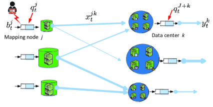
For compactness, collect the data workloads across edges $e=(i,j)\in{\cal E}$ in a resource allocation vector $\mathbf{x}_{t}:=[x_{t}^{11},\ldots,x_{t}^{JK},y_{t}^{1},\ldots,y_{t}^{K}]^{\top}\in\mathbb{R}^{E}_{+}$, and the exogenous load arrival rates of all nodes in a vector $\mathbf{b}_{t}:=[b_{t}^{1},\ldots,b_{t}^{J},0\ldots,0]^{\top}\in\mathbb{R}_{+}^{I}$. Then, the aggregate (endogenous plus exogenous) workloads of all nodes are given by $\mathbf{A}\mathbf{x}_{t}+\mathbf{b}_{t}$. When the $i$-th entry of $\mathbf{A}\mathbf{x}_{t}+\mathbf{b}_{t}$ is positive, there is service residual at node $i$; otherwise, node $i$ over-serves the current workload arrival. Assume that each data center and mapping node has a local data queue to buffer unserved workloads [25]. With $\mathbf{q}_{t}:=[q_{t}^{1},\ldots,q_{t}^{J+K}]^{\top}$ collecting the queue lengths at each mapping node and data center, the queue update is $\mathbf{q}_{t+1}=\left[\mathbf{q}_{t}+\mathbf{A}\mathbf{x}_{t}+\mathbf{b}_{t}\right]^{+}$, where $[\,\cdot\,]^{+}$ ensures that the queue length is always non-negative. The bandwidth limit of link $(j,k)$ is $\bar{x}^{jk}$, and the resource capability of data center $k$ is $\bar{y}^{k}$, which can be compactly expressed by $\mathbf{x}\in{\cal X}$ with ${\cal X}:=\{\mathbf{0}\leq\mathbf{x}\leq\bar{\mathbf{x}}\}$ and $\bar{\mathbf{x}}:=[\bar{x}^{11},\ldots,\bar{x}^{JK},\bar{y}^{1},\ldots,\bar{y}^{K}]^{\top}$. The overall system diagram is depicted in Fig. 1.

For each data center, the power cost $f_{t}^{k}(y_{t}^{k}):=f^{k}(y_{t}^{k};\theta_{t}^{k})$ depends on a time-varying parameter $\theta_{t}^{k}$, which captures the energy price and the renewable generation at data center $k$ during slot $t$. The bandwidth cost $f_{t}^{jk}(x_{t}^{jk}):=f^{jk}(x_{t}^{jk};\theta_{t}^{jk})$ characterizes the transmission delay and is parameterized by a time-varying scalar $\theta_{t}^{jk}$. Scalars $\theta_{t}^{k}$ and $\theta_{t}^{jk}$ can be readily extended to vector forms. To keep the exposition simple, we use scalars to represent time-varying factors at nodes and edges.

Per slot $t$, the instantaneous cost $f_{t}(\mathbf{x}_{t})$ aggregates the costs of power consumed at all data centers plus the bandwidth costs at all links, namely

$$f_{t}(\mathbf{x}_{t}):=\sum_{k\in{\cal K}}~{}\underbrace{~{}~{}f_{t}^{k}(y_{t}^{k})~{}~{}}_{\rm power~{}cost}~{}+~{}\sum_{j\in{\cal J}}\sum_{k\in{\cal K}}~{}\underbrace{~{}~{}f_{t}^{jk}(x_{t}^{jk})~{}~{}}_{\rm bandwidth~{}cost}$$ (33)

where the objective can be also written as $f_{t}(\mathbf{x}_{t}):=f(\mathbf{x}_{t};\bm{\theta}_{t})$ with $\bm{\theta}_{t}:=[\theta_{t}^{1},\ldots,\theta_{t}^{K},\theta_{t}^{11},\ldots,\theta_{t}^{JK}]^{\top}$ concatenating all time-varying parameters. Aiming to minimize the accumulated cost while serving all workloads, the optimal workload routing and allocation strategy in this cloud network is the solution of the following optimization problem

$\displaystyle\min_{\{\mathbf{x}_{t}\in{\cal X},\forall t\}}\,\sum_{t=1}^{T}f_{t}(\mathbf{x}_{t})~{}~{}~{}\text{s. t.}~{}~{}$ $\displaystyle\mathbf{q}_{t+1}=\left[\mathbf{q}_{t}+\mathbf{A}\mathbf{x}_{t}+\mathbf{b}_{t}\right]^{+},\,\forall t$
$\displaystyle\mathbf{q}_{1}\geq\mathbf{0},~{}\mathbf{q}_{T+1}=\mathbf{0}$ (34)

where $\mathbf{q}_{1}$ is the given initial queue length, and $\mathbf{q}_{T+1}=\mathbf{0}$ guarantees that all workloads arrived have been served at the end of the scheduling horizon. Note that (IV-A) is time-coupled, and generally challenging to solve without information of future workload arrivals and time-varying cost functions. Therefore, we reformulate (IV-A) to fit our OCO formulation (1) by relaxing the queue recursion in (IV-A), namely

$$\mathbf{q}_{T+1}\geq\mathbf{q}_{T}+\mathbf{A}\mathbf{x}_{T}+\mathbf{b}_{T}\geq\mathbf{q}_{1}+\sum_{t=1}^{T}(\mathbf{A}\mathbf{x}_{t}+\mathbf{b}_{t})$$ (35)

which readily leads to $\sum_{t=1}^{T}(\mathbf{A}\mathbf{x}_{t}+\mathbf{b}_{t})\leq\mathbf{q}_{T+1}-\mathbf{q}_{1}\leq\mathbf{0}$, since $\mathbf{q}_{1}\geq\mathbf{0}$ and $\mathbf{q}_{T+1}=\mathbf{0}$. Therefore, instead of solving (IV-A), we aim to tackle a relaxed problem that is in the form of OCO with long-term constraints, given by

$\displaystyle\min_{\{\mathbf{x}_{t}\in{\cal X},\forall t\}}\,$ $\displaystyle\sum_{t=1}^{T}f_{t}(\mathbf{x}_{t})~{}~{}~{}\text{s. t.}~{}~{}\sum_{t=1}^{T}\left(\mathbf{A}\mathbf{x}_{t}+\mathbf{b}_{t}\right)\leq\mathbf{0}$ (36)

where the workload flow conservation constraint $\mathbf{A}\mathbf{x}_{t}+\mathbf{b}_{t}\leq\mathbf{0}$ must be satisfied in the long term rather than slot-by-slot. Clearly, (36) is in the form of (1). Therefore, the MOSP algorithm of Section III can be leveraged to solve (36) in an online fashion, with provable performance and feasibility guarantees. Specifically, with $\mathbf{g}_{t}(\mathbf{x}_{t})=\mathbf{A}\mathbf{x}_{t}+\mathbf{b}_{t}$, the primal update (8) boils down to a simple gradient update $\mathbf{x}_{t}\!=\!{\cal P}_{\cal X}\left(\mathbf{x}_{t-1}-\alpha\nabla f_{t-1}(\mathbf{x}_{t-1})-\alpha\mathbf{A}^{\top}\bm{\lambda}_{t}\right)$, where ${\cal P}_{\cal X}\left(\cdot\right)$ defines projection onto the convex set ${\cal X}$. The dual update (9) is $\bm{\lambda}_{t+1}\!=\!\big{[}\bm{\lambda}_{t}+\mu(\mathbf{A}\mathbf{x}_{t}+\mathbf{b}_{t})\big{]}^{+}\!$, which can be nicely regarded as a scaled version of the relaxed queue dynamics in (IV-A), with $\mathbf{q}_{t}=\bm{\lambda}_{t}/\mu$.

In addition to simple closed-form updates, MOSP can also afford a fully decentralized implementation by exploiting the problem structure of network resource allocation, where each mapping node or data center decides the amounts on all its outgoing links, and only exchanges information with its one-hop neighbors. Per time slot $t$, the primal update at mapping node $j$ includes variables on all its outgoing links, given by

$$x_{t}^{jk}\!=\!\left[x_{t-1}^{jk}\!-\!\alpha\nabla f^{jk}_{t-1}(x_{t-1}^{jk})\!-\!\alpha\left(\lambda_{t}^{k}\!-\!\lambda_{t}^{j}\right)\right]_{0}^{\bar{x}^{jk}}\!\!\!,\;\forall k\in{\cal K}$$ (37a)
and the dual update reduces to
$$\lambda_{t+1}^{j}=\left[\lambda_{t}^{j}+\mu\left(b_{t}^{j}-\sum_{k\in{\cal K}}x_{t}^{jk}\right)\right]^{+}.$$ (37b)
Likewise, for data center $k$, the primal update becomes
$$y_{t}^{k}=\left[y_{t-1}^{k}-\alpha\nabla f^{k}_{t-1}(y_{t-1}^{k})-\alpha\sum_{j\in{\cal J}}(\lambda_{t}^{k}-\lambda_{t}^{j})\right]_{0}^{\bar{y}^{k}}$$ (37c)
where $[\;\cdot\;]_{0}^{\bar{y}^{k}}\!\!:=\min\{\bar{y}^{k},\max\{\cdot\,,0\}\}$, and the dual recursion is
$$\lambda_{t+1}^{k}=\left[\lambda_{t}^{k}+\mu\left(\sum_{j\in{\cal J}}x_{t}^{jk}-y_{t}^{k}\right)\right]^{+}.$$ (37d)

Distributed MOSP for online network resource allocation is summarized in Algorithm 2.

Algorithm 2 ​Distributed MOSP for network resource allocation
1:Initialize: primal iterate $\mathbf{x}_{0}$, dual iterate $\bm{\lambda}_{1}$, and proper stepsizes $\alpha$ and $\mu$.
2:for $t=1,2\dots$ do
3:     Each mapping node $j$ performs (37a) and each data ccc center $k$ runs (37c).
4:     Mapping nodes and data centers observe local costs ccc and workload arrivals.
5:     Each mapping node $j$ performs (37b) and each data ccc center $k$ performs (37d).
6:     Mapping nodes (data centers) send multipliers to all ccc neighboring data centers (mapping nodes).
7:end for

IV-B Revisiting stochastic dual (sub)gradient

The dynamic network resource allocation problem in Section IV-A has so far been studied in the stochastic setting [32, 30]. Classical approaches include Lyapunov optimization [24, 25] and the stochastic dual (sub)gradient method [26], both of which rely on stochastic approximation (SA) [27]. In the context of stochastic optimization, the time-varying vectors $\{\bm{\xi}_{t}\}$ with $\bm{\xi}_{t}\!:=\![\bm{\theta}_{t}^{\top},\mathbf{b}_{t}^{\top}]^{\top}$ appearing in the cost and constraint are assumed to be independent realizations of a random variable $\bm{\Xi}$.333Extension is also available when $\{\bm{\xi}_{t}\}$ constitute a sample path from an ergodic stochastic process $\{\bm{\Xi}_{t}\}$, which converges to a stationary distribution; see e.g., [29, 33]. In an SA-based stochastic optimization algorithm, per time $t$, a policy first observes a realization $\bm{\xi}_{t}$ of the random variable $\bm{\Xi}$, and then (stochastically) selects an action $\mathbf{x}_{t}\in{\cal X}$. However, in contrast to minimizing the observed cost in the OCO setting, the goal of the stochastic resource allocation is usually to minimize the limiting average of the expected cost subject to the so-termed stability constraint, namely

$\displaystyle\min_{\{\mathbf{x}_{t}\in{\cal X},\mathbf{q}_{t},\forall t\}}\,$ $\displaystyle\lim_{T\rightarrow\infty}\frac{1}{T}\sum_{t=1}^{T}\mathbb{E}[f_{t}(\mathbf{x}_{t})]$ (38a)
s. t. $\displaystyle\mathbf{q}_{t+1}=\left[\mathbf{q}_{t}+\mathbf{A}\mathbf{x}_{t}+\mathbf{b}_{t}\right]^{+}\!,~{}\forall t$ (38b)
$\displaystyle\lim_{T\rightarrow\infty}\frac{1}{T}\sum_{t=1}^{T}\mathbb{E}\left[\mathbf{q}_{t}\right]\leq\mathbf{0}$ (38c)

where he expectation in (38a) is taken over $\bm{\Xi}$ and the randomness of $\mathbf{x}_{t}$ and $\mathbf{q}_{t}$ induced by all possible sample paths $\{\bm{\xi}_{1},\ldots,\bm{\xi}_{t}\}$ via (38b); and the stability constraint (38c) implies a finite bound on the accumulated constraint violation. In contrast to the observed costs in (IV-A), each decision $\mathbf{x}_{t}$ is evaluated by all possible realizations in $\bm{\Xi}$ here. However, as $\mathbf{q}_{t}$ in (38b) couples the optimization variables over an infinite time horizon, (38) is intractable in general.

Prior works [25, 34, 26, 30] have demonstrated that (38) can be tackled via a tractable stationary relaxation, given by

$\displaystyle\min_{\{\mathbf{x}_{t}\in{\cal X},\forall t\}}\,$ $\displaystyle\lim_{T\rightarrow\infty}\frac{1}{T}\sum_{t=1}^{T}\mathbb{E}[f_{t}(\mathbf{x}_{t})]$ (39a)
s. t. $\displaystyle\lim_{T\rightarrow\infty}\frac{1}{T}\sum_{t=1}^{T}\mathbb{E}\left[\mathbf{A}\mathbf{x}_{t}+\mathbf{b}_{t}\right]\leq\mathbf{0}$ (39b)

where the time-coupling constraints (38b) and (38c) are relaxed to the limiting average constraint (39b). Such a relaxation can be verified similar to the queue relaxation in (35); see also [25]. Note that (39) is still challenging since it involves expectations in both costs and constraints, and the distribution of $\bm{\Xi}$ is usually unknown. Even if the joint probability distribution function were available, finding the expectations would not scale with the dimensionality of $\bm{\Xi}$. A common remedy is to use the stochastic dual gradient (SDG) iteration (a.k.a. Lyapunov optimization) [24, 25, 30]. Specifically, with $\bm{\lambda}\in\mathbb{R}_{+}^{I}$ denoting the multipliers associated with the expectation constraint (39b), the SDG method first observes one realization $\bm{\xi}_{t}$ at each slot $t$, and then performs the dual update as

$\displaystyle\bm{\lambda}_{t+1}~{}=\big{[}\bm{\lambda}_{t}+\mu(\mathbf{A}\mathbf{x}_{t}+\mathbf{b}_{t})\big{]}^{+},\;\forall t$ (40)

where $\bm{\lambda}_{t}$ is the dual iterate at time $t$, $\mathbf{A}\mathbf{x}_{t}+\mathbf{b}_{t}$ is the stochastic dual gradient, and $\mu$ is a positive (and typically constant) stepsize. The actual allocation or the primal variable $\mathbf{x}_{t}$ appearing in (40) needs be found by solving the following sub-problems, one per slot $t$

$\displaystyle\mathbf{x}_{t}\in\arg\min_{\mathbf{x}\in{\cal X}}f_{t}(\mathbf{x})+\bm{\lambda}_{t}^{\top}(\mathbf{A}\mathbf{x}+\mathbf{b}_{t}).$ (41)

For the considered network resource allocation problem, SDG in (40)-(41) entails a well-known cost-delay tradeoff [25]. Specifically, with $f^{*}$ denoting the optimal objective (39), SDG can achieve an ${\cal O}(\mu)$-optimal solution such that $\lim_{T\rightarrow\infty}({1}/{T})\sum_{t=1}^{T}\mathbb{E}\left[f_{t}\left(\mathbf{x}_{t}\right)\right]\!\leq\!f^{*}\!+{\cal O}(\mu)$, and guarantee queue lengths444According to Little’s law [35], the time-average delay is proportional to the time-average queue length given the arrival rate. satisfying $\lim_{T\rightarrow\infty}({1}/{T})\sum_{t=1}^{T}\mathbb{E}\left[\|\mathbf{q}_{t}\|\right]\!=\!{\cal O}({1}/{\mu})$. Therefore, reducing the optimality gap ${\cal O}(\mu)$ will essentially increase the average network delay ${\cal O}(1/\mu)$.

Remark 4.

The optimality of SDG is established relative to the offline optimal solution of (39), which can be thought as the time-average optimality gap in (22a) under the OCO setting. Interestingly though, the optimality gap under the stochastic setting is equivalent to the (expected) dynamic regret (4), since their (expected) difference $V(\{\mathbb{E}[{\cal D}_{t}]\}_{t=1}^{T})$ in (28) reduces to zero. To see this, note that $\mathbb{E}[f_{t}(\mathbf{x})]$ and $\mathbb{E}[\mathbf{A}\mathbf{x}+\mathbf{b}_{t}]$ are time-invariant, hence the dual problem of each per-slot subproblem in (39) is time-invariant. This reduction means that the SDG solver of the dynamic problem in (38) leverages its inherent stationarity (through the stationary dual problem), in contrast to the non-stationary nature of the OCO framework.

Remark 5.

Below we highlight several differences of the novel MOSP in Algorithm 2 with the SDG recursion in (40)-(41) for the dynamic network resource allocation task.

(D1) From an operational perspective, SDG observes the current state $\bm{\xi}_{t}$ first, and then performs the resource allocation decision $\mathbf{x}_{t}$ accordingly. Therefore, at the beginning of slot $t$, SDG needs to precisely know the non-causal information $\bm{\xi}_{t}$. Inheriting the merits of OCO, on the other hand, MOSP operates in a fully predictive mode, which decides $\mathbf{x}_{t}$ without knowing the cost $f_{t}(\mathbf{x})$ and the constraint $\mathbf{g}_{t}(\mathbf{x})$ (or $\bm{\xi}_{t}$) at time $t$. This feature of MOSP is of major practical importance when costs and availability of resources are not available at the point of making decisions; e.g., online demand response in smart grids [36] and resource allocation in wireless networking [37].

(D2) From a computational point of view, MOSP reduces to a simple saddle-point recursion with primal (projected) gradient descent and dual gradient ascent for the network resource allocation problem, both of which incur affordable complexity. However, the primal update of SDG in (41) generally requires solving a convex program per time slot $t$, which leads to much higher computational complexity in general.

(D3) With regards to the theoretical claims, the time-varying vector $\bm{\xi}_{t}$ in SDG typically requires a rather restrictive probabilistic assumption, to establish SDG optimality in either the ensemble average [25] or the limiting ergodic average sense [33]. In contrast, leveraging the OCO framework, MOSP admits finite-sample performance analysis with non-stochastic observed costs and constraints, which can even be adversarial.

IV-C Numerical experiments

In this section, we provide numerical tests to demonstrate the merits of the proposed MOSP algorithm in the application of dynamic network resource allocation. Consider the geographical workload routing and allocation task in (36) with $J=10$ mapping nodes and $K=10$ data centers. The instantaneous network cost in (33) is

$$f_{t}(\mathbf{x}_{t})\!:=\sum_{k\in{\cal K}}p_{t}^{k}(y_{t}^{k})^{2}+\sum_{j\in{\cal J}}\sum_{k\in{\cal K}}c^{jk}(x_{t}^{jk})^{2}$$ (42)

where $p_{t}^{k}$ is the energy price at data center $k$ at time $t$, and $c^{jk}$ is the per-unit bandwidth cost for transmitting from mapping node $j$ to data center $k$. With the bandwidth limit $\bar{x}^{jk}$ uniformly randomly generated within $[10,100]$, we set the bandwidth cost of each link $(j,k)$ as $c^{jk}=40/\bar{x}^{jk},\forall j,k$. The resource capacities $\{\bar{y}^{k},\forall k\}$ at all data centers are uniformly randomly generated from $[100,200]$. We consider the following two cases for the time-varying parameters $\{p_{t}^{k},\forall t,k\}$ and $\{b_{t}^{j},\forall t,j\}$:

Case 1) Parameters $\{p_{t}^{k},\forall t,k\}$ and $\{b_{t}^{j},\forall t,j\}$ are independently drawn from time-invariant distributions. Specifically, $p_{t}^{k}$ is uniformly distributed over $[1,3]$, and the delay-tolerant workload $b_{t}^{j}$ arrives at each mapping node $j$ according to a uniform distribution over $[50,150]$.

Case 2) Parameters $\{p_{t}^{k},\forall t,k\}$ and $\{b_{t}^{j},\forall t,j\}$ are generated according to non-stationary stochastic processes. Specifically, $p_{t}^{k}=\sin(\pi t/12)+n_{t}^{k}$ with i.i.d. noise $n_{t}^{k}$ uniformly distributed over $[1,3]$, while $b_{t}^{j}=50\sin(\pi t/12)+v_{t}^{j}$ with i.i.d. noise $v_{t}^{j}$ uniformly distributed over $[99,101]$.

Finally, with time horizon $T=500$, the stepsize in (37a) and (37c) is set to $\alpha=0.05/T^{1/3}$, and for (37b) and (37d) to $\mu=50/T^{1/3}$. MOSP is benchmarked by three strategies: SDG in Section IV-B, the sequence of per-slot best minimizers in (3), and the offline optimal solution that solves (1) at once with all future costs and constraints available. Note that at the beginning of each slot $t$, the exact prices $\{p_{t}^{k},\forall k\}$ and demands $\{b_{t}^{j},\forall j\}$ for the coming slot are generally not available in practice [38, 36, 37, 39]. Since the original SDG updates (40) and (41) require non-causal knowledge of $\{p_{t}^{k},\forall k\}$ and $\{b_{t}^{j},\forall j\}$ to decide $\mathbf{x}_{t}$, we modify them for fairness in this online setting by using the prices and demands at slot $t-1$ to obtain $\mathbf{x}_{t}$. In this case that we we term online dual gradient (ODG), the performance guarantee of SDG may not hold. Nevertheless, as shown in the next, different constant stepsizes for ODG’s dual update in (40) still lead to quite different performance and feasibility behaviors. For this reason, ODG is studied under stepsizes $\mu_{\rm ODG}=0.5$ and $1$.

Refer to caption
Figure 2: Time-average cost for Case 1.
Refer to caption
Figure 3: Dynamic regret for Case 1.
Refer to caption
Figure 4: Dynamic fit for Case 1.
Refer to caption
Figure 5: Time-average cost for Case 2.

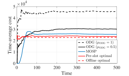
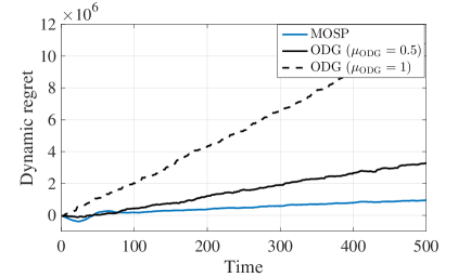
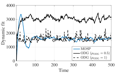
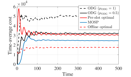
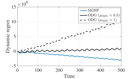
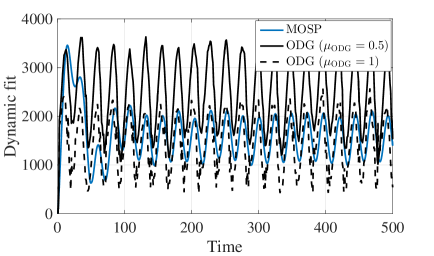
Figs. 2-4 show the test results for Case 1 under i.i.d. costs and constraints. Clearly, MOSP in Fig. 2 converges to a smaller time-average cost than ODG with the two stepsizes. The time-average cost of MOSP is slightly higher than the per-slot optimal solution, as well as the offline optimal solution with all information of the costs and constraints available over horizon $T$. Fig. 3 confirms the conclusion made from Fig. 2, where the dynamic regret (cf. (4)) of MOSP grows much slower than that of ODG. Regarding the dynamic fit (cf. (6)), Fig. 4 demonstrates that ODG with $\mu_{\rm ODG}=1$ has a smaller fit than that of $\mu_{\rm ODG}=0.5$, and similar to the dynamic fit of MOSP. According to the well-known trade-off between cost (optimality) and delay (constraint violations) in [25], increasing $\mu_{\rm ODG}$ will improve the dynamic fit of ODG but degrade its dynamic regret. Therefore, MOSP is favorable in Case 1 since it has much smaller regret when its dynamic fit is similar to that of ODG with $\mu_{\rm ODG}=1$. It is worth mentioning that theoretically speaking, the dynamic regret of MOSP may not be sub-linear in this i.i.d. case, since the accumulated cost and constraint variation is not necessarily small enough (cf. Theorem 2). However, MOSP is robust in this aspect at least for the numerical tests we carried.

Refer to caption
Figure 6: Dynamic regret for Case 2.
Refer to caption
Figure 7: Dynamic fit for Case 2.

Simulation tests using non-stationary costs and constraints are shown in Figs. 5-7. Different from Case 1, the time-average cost of MOSP is not only smaller than ODG, but also smaller than the per-slot optimum obtained via (3); see Fig. 5. A similar conclusion can be also drawn through the growths of dynamic regret in Fig. 6. From a high level, this is because the difference between the cost of the per-slot minimizers and that of the offline solutions is no longer small in the non-stationary case. Regarding Fig. 7, both ODG and MOSP have finite dynamic fits in the sense that the accumulated constraint violations do not increase with time. The dynamic fit of MOSP is much smaller than that of ODG with $\mu_{\rm ODG}=0.5$, and comparable to that of ODG with $\mu_{\rm ODG}=1$. Therefore, in this non-stationary case, MOSP also significantly outperforms ODG in both dynamic regret and fit.

V Concluding Remarks

OCO with both adversarial costs and constraints has been studied in this paper. Different from existing works, the focus is on a setting where some of the constraints are revealed after taking actions, they are tolerable to instantaneous violations, but must be satisfied on average. Performance of the novel OCO algorithm is measured by: i) the difference of its objective relative to the best dynamic solution with one-slot-ahead information of the cost and the constraint (dynamic regret); and, ii) its accumulated amount of constraint violations (dynamic fit). It has been shown that the proposed MOSP algorithm adapts to the considered OCO setting with adversarial constraints. Under standard assumptions, MOSP simultaneously yields sub-linear dynamic regret and fit, if the accumulated variations of the per-slot minimizers and adversarial constraints are sub-linearly increasing with time. Algorithm design and performance analysis in this novel OCO setting, under adversarial constraints and with a dynamic benchmark, broaden the applicability of OCO to a wider application regime, which includes dynamic network resource allocation and online demand response in smart grids. Numerical tests demonstrated that the proposed algorithm outperforms state-of-the-art alternatives under different scenarios.

Acknowledgement

The authors would like to thank Prof. Xin Wang for helpful discussions and comments.

Before proving Theorems 1 and 2, we first bound the variation of the dual variable for the MOSP recursion (8)-(9). With the dual drift defined as $\Delta(\bm{\lambda}_{t}):=\left(\|\bm{\lambda}_{t+1}\|^{2}-\|\bm{\lambda}_{t}\|^{2}\right)/2$, we have the following lemma.

Lemma 1.

Per slot $t$, the dual drift of the MOSP recursion (8)-(9) is upper-bounded as

$\displaystyle\Delta(\bm{\lambda}_{t})\leq\mu\bm{\lambda}_{t}^{\top}\mathbf{g}_{t}(\mathbf{x}_{t})+\frac{\mu^{2}}{2}\|\mathbf{g}_{t}(\mathbf{x}_{t})\|^{2}.$ (43)
Proof.

Squaring the dual variable update (9), we have

$\displaystyle\|\bm{\lambda}_{t+1}\|^{2}$ $\displaystyle=\left\|\big{[}\bm{\lambda}_{t}+\mu\mathbf{g}_{t}(\mathbf{x}_{t})\big{]}^{+}\right\|^{2}\leq\left\|\bm{\lambda}_{t}+\mu\mathbf{g}_{t}(\mathbf{x}_{t})\right\|^{2}$
$\displaystyle=\|\bm{\lambda}_{t}\|^{2}+2\mu\bm{\lambda}_{t}^{\top}\mathbf{g}_{t}(\mathbf{x}_{t})+\mu^{2}\|\mathbf{g}_{t}(\mathbf{x}_{t})\|^{2}.$ (44)

And the proof is complete after rearranging terms and dividing both sides by 2. ∎

-A Proof of Theorem 1

The proof follows the steps in [12, Theorem 7], but generalizes the result from static regret with time-invariant constraints to dynamic regret with time-varying and long-term constraints. Recall that the primal iterate $\mathbf{x}_{t+1}$ is the optimal solution to the following optimization problem (cf. (8))

$$\min_{\mathbf{x}\in{\cal X}}\;\nabla^{\top}f_{t}(\mathbf{x}_{t})\!\left(\mathbf{x}-\mathbf{x}_{t}\right)+\bm{\lambda}_{t+1}^{\top}\mathbf{g}_{t}(\mathbf{x})+\frac{1}{2\alpha}\|\mathbf{x}-\mathbf{x}_{t}\|^{2}.$$

Then for any interior point $\tilde{\mathbf{x}}_{t}\in{\cal X}$ in Assumption 4, it follows that

$\displaystyle\nabla^{\top}f_{t}(\mathbf{x}_{t})\!\left(\mathbf{x}_{t+1}\!-\!\mathbf{x}_{t}\right)+\bm{\lambda}_{t+1}^{\top}\mathbf{g}_{t}(\mathbf{x}_{t+1})\!+\!\frac{1}{2\alpha}\|\mathbf{x}_{t+1}\!-\!\mathbf{x}_{t}\|^{2}$
$\displaystyle\leq$ $\displaystyle\nabla^{\top}f_{t}(\mathbf{x}_{t})\!\left(\tilde{\mathbf{x}}_{t}\!-\!\mathbf{x}_{t}\right)+\bm{\lambda}_{t+1}^{\top}\mathbf{g}_{t}(\tilde{\mathbf{x}}_{t})+\frac{1}{2\alpha}\|\tilde{\mathbf{x}}_{t}\!-\!\mathbf{x}_{t}\|^{2}$
$\displaystyle\stackrel{{\scriptstyle(a)}}{{\leq}}$ $\displaystyle\nabla^{\top}f_{t}(\mathbf{x}_{t})\!\left(\tilde{\mathbf{x}}_{t}\!-\!\mathbf{x}_{t}\right)-\epsilon\bm{\lambda}_{t+1}^{\top}\mathbf{1}+\frac{1}{2\alpha}\|\tilde{\mathbf{x}}_{t}\!-\!\mathbf{x}_{t}\|^{2}$
$\displaystyle\stackrel{{\scriptstyle(b)}}{{\leq}}$ $\displaystyle\nabla^{\top}f_{t}(\mathbf{x}_{t})\!\left(\tilde{\mathbf{x}}_{t}\!-\!\mathbf{x}_{t}\right)-\epsilon\|\bm{\lambda}_{t+1}\|+\frac{1}{2\alpha}\|\tilde{\mathbf{x}}_{t}\!-\!\mathbf{x}_{t}\|^{2}$ (45)

where (a) follows by choosing $\tilde{\mathbf{x}}_{t}$ such that $\mathbf{g}_{t}(\tilde{\mathbf{x}}_{t})\leq-\epsilon\mathbf{1}$ and recalling the non-negativity of $\bm{\lambda}_{t+1}$; inequality (b) is because $\|\bm{\lambda}_{t+1}\|\leq\bm{\lambda}_{t+1}^{\top}\mathbf{1}$ holds for any non-negative vector $\bm{\lambda}_{t+1}$.

Rearranging terms in (-A), it follows that

$\displaystyle\bm{\lambda}_{t+1}^{\top}\mathbf{g}_{t}(\mathbf{x}_{t+1})\leq\nabla^{\top}f_{t}(\mathbf{x}_{t})\!\left(\tilde{\mathbf{x}}_{t}-\mathbf{x}_{t}\right)\!-\!\nabla^{\top}f_{t}(\mathbf{x}_{t})\!\left(\mathbf{x}_{t+1}-\mathbf{x}_{t}\right)$
$\displaystyle\qquad\qquad\qquad\quad-\epsilon\|\bm{\lambda}_{t+1}\|\!+\!\frac{1}{2\alpha}\|\tilde{\mathbf{x}}_{t}-\mathbf{x}_{t}\|^{2}\!-\!\frac{1}{2\alpha}\|\mathbf{x}_{t+1}-\mathbf{x}_{t}\|^{2}$
$\displaystyle\stackrel{{\scriptstyle(c)}}{{\leq}}\!\nabla^{\top}f_{t}(\mathbf{x}_{t})\!\left(\tilde{\mathbf{x}}_{t}-\mathbf{x}_{t}\right)\!-\!\nabla^{\top}f_{t}(\mathbf{x}_{t})\!\left(\mathbf{x}_{t+1}-\mathbf{x}_{t}\right)\!-\!\epsilon\|\bm{\lambda}_{t+1}\|\!+\!\frac{R^{2}}{2\alpha}$
$\displaystyle\stackrel{{\scriptstyle(d)}}{{\leq}}\!\!\|\nabla f_{t}(\mathbf{x}_{t})\|\|\tilde{\mathbf{x}}_{t}\!-\!\mathbf{x}_{t}\|\!+\!\|\nabla f_{t}(\mathbf{x}_{t})\|\|\mathbf{x}_{t+1}\!-\!\mathbf{x}_{t}\|\!-\!\epsilon\|\bm{\lambda}_{t+1}\|\!+\!\frac{R^{2}}{2\alpha}$
$\displaystyle\stackrel{{\scriptstyle(e)}}{{\leq}}2GR-\epsilon\|\bm{\lambda}_{t+1}\|+\frac{R^{2}}{2\alpha}$ (46)

where (c) holds since ${\cal X}$ confines $\|\tilde{\mathbf{x}}_{t}-\mathbf{x}_{t}\|^{2}\leq R^{2}$ and $\|\mathbf{x}_{t+1}-\mathbf{x}_{t}\|^{2}\geq 0$; (d) uses the Cauchy-Schwartz inequality twice; (e) leverages the bounds in Assumption 3, namely, $\|\nabla f_{t}(\mathbf{x}_{t})\|\leq G$, $\|\tilde{\mathbf{x}}_{t}-\mathbf{x}_{t}\|\leq R$, and $\|\mathbf{x}_{t+1}\!-\!\mathbf{x}_{t}\|\leq R$.

Plugging (-A) into (Proof.) in Lemma 1, we have

$\displaystyle\Delta(\bm{\lambda}_{t+1})\leq\mu\bm{\lambda}_{t+1}^{\top}\mathbf{g}_{t+1}(\mathbf{x}_{t+1})+\frac{\mu^{2}}{2}\|\mathbf{g}_{t+1}(\mathbf{x}_{t+1})\|^{2}$
$\displaystyle\stackrel{{\scriptstyle(f)}}{{\leq}}\mu\bm{\lambda}_{t+1}^{\top}\big{(}\mathbf{g}_{t+1}(\mathbf{x}_{t+1})-\mathbf{g}_{t}(\mathbf{x}_{t+1})\big{)}-\epsilon\mu\|\bm{\lambda}_{t+1}\|$
$\displaystyle\qquad\qquad\qquad\qquad\qquad\qquad\qquad~{}~{}+2\mu GR+\frac{\mu R^{2}}{2\alpha}+\frac{\mu^{2}M^{2}}{2}$
$\displaystyle\stackrel{{\scriptstyle(g)}}{{\leq}}\mu\bm{\lambda}_{t+1}^{\top}\big{[}\mathbf{g}_{t+1}(\mathbf{x}_{t+1})-\mathbf{g}_{t}(\mathbf{x}_{t+1})\big{]}^{+}\!\!\!-\epsilon\mu\|\bm{\lambda}_{t+1}\|$
$\displaystyle\qquad\qquad\qquad\qquad\qquad\qquad\qquad~{}~{}+2\mu GR+\frac{\mu R^{2}}{2\alpha}+\frac{\mu^{2}M^{2}}{2}$
$\displaystyle\stackrel{{\scriptstyle(h)}}{{\leq}}\mu\bar{V}(\mathbf{g})\|\bm{\lambda}_{t+1}\|\!-\!\epsilon\mu\|\bm{\lambda}_{t+1}\|\!+\!2\mu GR\!+\!\frac{\mu R^{2}}{2\alpha}\!+\!\frac{\mu^{2}M^{2}}{2}\!\!\!$ (47)

where (f) uses the upper bound in Assumption 2 such that $\|\mathbf{g}_{t+1}(\mathbf{x}_{t+1})\|\leq M$, (g) holds since $\bm{\lambda}_{t+1}\geq\mathbf{0}$, and (h) follows from the Cauchy-Schwartz inequality and the definition of the maximum variation $\bar{V}(\mathbf{g})$ in (10).

We prove the dual upper bound (11) by contradiction. Without loss of generality, suppose that $t+2$ is the first time that (11) does not hold. Therefore, we have

$$\|\bm{\lambda}_{t+1}\|\leq\|\bar{\bm{\lambda}}\|=\mu M+\frac{2GR+{R^{2}}/(2\alpha)+(\mu M^{2})/{2}}{\epsilon-\bar{V}(\mathbf{g})}$$ (48a)
and correspondingly
$$\|\bm{\lambda}_{t+2}\|>\|\bar{\bm{\lambda}}\|=\mu M+\frac{2GR+{R^{2}}/(2\alpha)+(\mu M^{2})/{2}}{\epsilon-\bar{V}(\mathbf{g})}.$$ (48b)

In this case, it follows that

$\displaystyle\|\bm{\lambda}_{t+1}\|$ $\displaystyle\geq\|\bm{\lambda}_{t+2}\|-\|\bm{\lambda}_{t+2}-\bm{\lambda}_{t+1}\|$
$\displaystyle=\|\bm{\lambda}_{t+2}\|-\|[\bm{\lambda}_{t+1}+\mu\mathbf{g}_{t+1}(\mathbf{x}_{t+1})]^{+}-\bm{\lambda}_{t+1}\|$
$\displaystyle\stackrel{{\scriptstyle(i)}}{{\geq}}\|\bm{\lambda}_{t+2}\|-\|\mu\mathbf{g}_{t+1}(\mathbf{x}_{t+1})\|$
$\displaystyle\stackrel{{\scriptstyle(j)}}{{>}}\frac{2GR+{R^{2}}/(2\alpha)+(\mu M^{2})/{2}}{\epsilon-\bar{V}(\mathbf{g})}$ (49)

where (i) is due to the non-expansive property of the projection operator, and inequality (j) uses (48b) and $\|\mathbf{g}_{t+1}(\mathbf{x}_{t+1})\|\leq M$ in Assumption 2. However, since $\epsilon>\bar{V}(\mathbf{g})$, (-A) implies that we have $\Delta(\bm{\lambda}_{t+1})<0$ if (-A) holds. By definition of the dual drift, $\Delta(\bm{\lambda}_{t+1})<0$ implies that $\|\bm{\lambda}_{t+2}\|<\|\bm{\lambda}_{t+1}\|$, which contradicts (48a) and (48b). In addition, observe that the dual variable is initialized by $\bm{\lambda}_{1}=\mathbf{0}$, and consequently $\|\bm{\lambda}_{2}\|\leq\mu M$. Therefore, for every $t$, we have that $\|\bm{\lambda}_{t}\|\leq\|\bar{\bm{\lambda}}\|$ holds.

Using the dual recursion in (9), it follows that $\bm{\lambda}_{T+1}\geq\bm{\lambda}_{T}+\mu\mathbf{g}_{T}(\mathbf{x}_{T})\geq\bm{\lambda}_{1}+\sum_{t=1}^{T}\mu\mathbf{g}_{t}(\mathbf{x}_{t})$. Rearranging terms, we have

$$\sum_{t=1}^{T}\mathbf{g}_{t}(\mathbf{x}_{t})\leq\frac{\bm{\lambda}_{T+1}}{\mu}-\frac{\bm{\lambda}_{1}}{\mu}\leq\frac{\bm{\lambda}_{T+1}}{\mu}.$$ (50)

With $\bm{\lambda}_{T+1}\geq\mathbf{0}$, (50) implies that $\left[\sum_{t=1}^{T}\mathbf{g}_{t}(\mathbf{x}_{t})\right]^{+}\!\!\leq{\bm{\lambda}_{T+1}}/{\mu}$, which completes the proof by taking norms on both sides and using the dual upper bound (11).

-B Proof of Theorem 2

Per slot $t$, the primal update $\mathbf{x}_{t+1}$ is the minimizer of the optimization problem in (8); hence,

$\displaystyle\nabla^{\top}f_{t}(\mathbf{x}_{t})\left(\mathbf{x}_{t+1}\!-\!\mathbf{x}_{t}\right)\!+\!\bm{\lambda}_{t+1}^{\top}\mathbf{g}_{t}(\mathbf{x}_{t+1})\!+\!\frac{\|\mathbf{x}_{t+1}\!-\!\mathbf{x}_{t}\|^{2}}{2\alpha}$ (51)
$\displaystyle\!\!\!\stackrel{{\scriptstyle(a)}}{{\leq}}$ $\displaystyle\nabla^{\top}\!\!f_{t}(\mathbf{x}_{t})(\mathbf{x}^{*}_{t}\!-\!\mathbf{x}_{t})\!+\!\bm{\lambda}_{t+1}^{\top}\mathbf{g}_{t}(\mathbf{x}_{t}^{*})\!+\!\frac{\|\mathbf{x}^{*}_{t}\!-\!\mathbf{x}_{t}\|^{2}}{2\alpha}\!-\!\frac{\|\mathbf{x}_{t+1}\!-\!\mathbf{x}^{*}_{t}\|^{2}}{2\alpha}$

where (a) uses the strong convexity of the objective in (8); see also [12, Corollary 1]. Adding $f_{t}(\mathbf{x}_{t})$ in (51) yields

$\displaystyle f_{t}(\mathbf{x}_{t})\!+\!\nabla^{\top}\!f_{t}(\mathbf{x}_{t})\left(\mathbf{x}_{t+1}\!-\!\mathbf{x}_{t}\right)\!+\!\bm{\lambda}_{t+1}^{\top}\mathbf{g}_{t}(\mathbf{x}_{t+1})\!+\!\frac{\|\mathbf{x}_{t+1}\!-\!\mathbf{x}_{t}\|^{2}}{2\alpha}$
$\displaystyle\leq$ $\displaystyle f_{t}(\mathbf{x}_{t})\!+\!\nabla^{\top}f_{t}(\mathbf{x}_{t})\left(\mathbf{x}^{*}_{t}\!-\!\mathbf{x}_{t}\right)\!+\!\bm{\lambda}_{t+1}^{\top}\mathbf{g}_{t}(\mathbf{x}_{t}^{*})$
$\displaystyle\qquad\qquad\qquad\qquad\qquad\qquad~{}\,+\frac{\|\mathbf{x}^{*}_{t}\!-\!\mathbf{x}_{t}\|^{2}}{2\alpha}-\frac{\|\mathbf{x}^{*}_{t}\!-\!\mathbf{x}_{t+1}\|^{2}}{2\alpha}$
$\displaystyle\stackrel{{\scriptstyle(b)}}{{\leq}}$ $\displaystyle f_{t}(\mathbf{x}^{*}_{t})+\bm{\lambda}_{t+1}^{\top}\mathbf{g}_{t}(\mathbf{x}_{t}^{*})\!+\!\frac{\|\mathbf{x}^{*}_{t}\!-\!\mathbf{x}_{t}\|^{2}}{2\alpha}\!-\!\frac{\|\mathbf{x}^{*}_{t}\!-\!\mathbf{x}_{t+1}\|^{2}}{2\alpha}$
$\displaystyle\stackrel{{\scriptstyle(c)}}{{\leq}}$ $\displaystyle f_{t}(\mathbf{x}^{*}_{t})+\frac{\|\mathbf{x}^{*}_{t}\!-\!\mathbf{x}_{t}\|^{2}}{2\alpha}-\frac{\|\mathbf{x}^{*}_{t}\!-\!\mathbf{x}_{t+1}\|^{2}}{2\alpha}$ (52)

where (b) is due to the convexity of $f_{t}(\mathbf{x})$, and (c) comes from the fact that $\bm{\lambda}_{t+1}\geq\mathbf{0}$ and the per-slot optimal solution $\mathbf{x}^{*}_{t}$ is feasible (i.e., $\mathbf{g}_{t}(\mathbf{x}_{t}^{*})\leq\mathbf{0}$) such that $\bm{\lambda}_{t+1}^{\top}\mathbf{g}_{t}(\mathbf{x}_{t}^{*})\leq 0$.

Next, we bound the term $\nabla^{\top}f_{t}(\mathbf{x}_{t})\left(\mathbf{x}_{t+1}\!-\!\mathbf{x}_{t}\right)$ by

$\displaystyle-\nabla^{\top}f_{t}(\mathbf{x}_{t})\left(\mathbf{x}_{t+1}\!-\!\mathbf{x}_{t}\right)\leq\|\nabla f_{t}(\mathbf{x}_{t})\|\|\mathbf{x}_{t+1}-\mathbf{x}_{t}\|$ (53)
$\displaystyle\leq$ $\displaystyle\frac{\|\nabla f_{t}(\mathbf{x}_{t})\|^{2}}{2\eta}+\frac{\eta}{2}\|\mathbf{x}_{t+1}\!-\!\mathbf{x}_{t}\|^{2}\stackrel{{\scriptstyle(d)}}{{\leq}}\frac{G^{2}}{2\eta}+\frac{\eta}{2}\|\mathbf{x}_{t+1}-\mathbf{x}_{t}\|^{2}$

where $\eta$ is an arbitrary positive constant, and (d) is from the bound of gradients in Assumption 2. Plugging (53) into (52), we have

$\displaystyle f_{t}(\mathbf{x}_{t})+\bm{\lambda}_{t+1}^{\top}\mathbf{g}_{t}(\mathbf{x}_{t+1})\leq f_{t}(\mathbf{x}^{*}_{t})+\Big{(}\frac{\eta}{2}-\frac{1}{2\alpha}\Big{)}\|\mathbf{x}_{t+1}\!-\!\mathbf{x}_{t}\|^{2}$
$\displaystyle\qquad~{}\,+\frac{1}{2\alpha}\Big{(}\|\mathbf{x}^{*}_{t}\!-\!\mathbf{x}_{t}\|^{2}\!-\!\|\mathbf{x}^{*}_{t}\!-\!\mathbf{x}_{t+1}\|^{2}\Big{)}+\frac{G^{2}}{2\eta}$
$\displaystyle\stackrel{{\scriptstyle(e)}}{{=}}$ $\displaystyle f_{t}(\mathbf{x}^{*}_{t})\!+\!\frac{1}{2\alpha}\Big{(}\|\mathbf{x}^{*}_{t}\!-\!\mathbf{x}_{t}\|^{2}\!-\!\|\mathbf{x}^{*}_{t}\!-\!\mathbf{x}_{t+1}\|^{2}\Big{)}\!+\!\frac{\alpha G^{2}}{2}$ (54)

where equality (e) follows by choosing $\eta=1/\alpha$ to obtain $\eta/2-1/(2\alpha)=0$.

Using the dual drift bound (43) in Lemma 1 again, we have

$\displaystyle\Delta(\bm{\lambda}_{t+1})/\mu+f_{t}(\mathbf{x}_{t})\leq f_{t}(\mathbf{x}_{t})+\bm{\lambda}_{t+1}^{\top}\mathbf{g}_{t}(\mathbf{x}_{t+1})$
$\displaystyle\qquad+\bm{\lambda}_{t+1}^{\top}\mathbf{g}_{t+1}(\mathbf{x}_{t+1})-\bm{\lambda}_{t+1}^{\top}\mathbf{g}_{t}(\mathbf{x}_{t+1})+\frac{\mu}{2}\|\mathbf{g}_{t+1}(\mathbf{x}_{t+1})\|^{2}$
$\displaystyle\stackrel{{\scriptstyle(f)}}{{\leq}}$ $\displaystyle f_{t}(\mathbf{x}^{*}_{t})\!+\!\frac{1}{2\alpha}\Big{(}\|\mathbf{x}^{*}_{t}\!-\!\mathbf{x}_{t}\|^{2}\!-\!\|\mathbf{x}^{*}_{t}\!-\!\mathbf{x}_{t+1}\|^{2}\Big{)}$
$\displaystyle+\!\bm{\lambda}_{t+1}^{\top}(\mathbf{g}_{t+1}(\mathbf{x}_{t+1})-\mathbf{g}_{t}(\mathbf{x}_{t+1}))\!+\!\frac{\mu\|\mathbf{g}_{t+1}(\mathbf{x}_{t+1})\|^{2}}{2}+\frac{\alpha G^{2}}{2}$
$\displaystyle\stackrel{{\scriptstyle(g)}}{{\leq}}$ $\displaystyle f_{t}(\mathbf{x}^{*}_{t})\!+\!\frac{1}{2\alpha}\Big{(}\|\mathbf{x}^{*}_{t}\!-\!\mathbf{x}_{t}\|^{2}\!-\!\|\mathbf{x}^{*}_{t}\!-\!\mathbf{x}_{t+1}\|^{2}\Big{)}$
$\displaystyle\qquad\qquad+\bm{\lambda}_{t+1}^{\top}\left[\mathbf{g}_{t+1}(\mathbf{x}_{t+1})-\mathbf{g}_{t}(\mathbf{x}_{t+1})\right]^{+}+\!\frac{\mu M^{2}}{2}\!+\frac{\alpha G^{2}}{2}$
$\displaystyle\stackrel{{\scriptstyle(h)}}{{\leq}}$ $\displaystyle f_{t}(\mathbf{x}^{*}_{t})\!+\!\frac{1}{2\alpha}\Big{(}\|\mathbf{x}^{*}_{t}\!-\!\mathbf{x}_{t}\|^{2}\!-\!\|\mathbf{x}^{*}_{t}\!-\!\mathbf{x}_{t+1}\|^{2}\Big{)}\!+\!\|\bm{\lambda}_{t+1}\|V(\mathbf{g}_{t})$
$\displaystyle\qquad\qquad+\frac{\mu M^{2}}{2}\!+\frac{\alpha G^{2}}{2}$ (55)

where (f) follows from (-B); (g) uses non-negativity of $\bm{\lambda}_{t+1}$ and the gradient upper bound $\|\mathbf{g}_{t+1}(\mathbf{x})\|\leq M,\forall\mathbf{x}\in{\cal X}$; and (h) follows from the Cauchy-Schwartz inequality and the definition of the constraint variation $V(\mathbf{g}_{t})$ in (10).

By interpolating intermediate terms in $\|\mathbf{x}^{*}_{t}\!-\!\mathbf{x}_{t}\|^{2}\!-\!\|\mathbf{x}^{*}_{t}\!-\!\mathbf{x}_{t+1}\|^{2}$, we have that

$\displaystyle\|\mathbf{x}^{*}_{t}\!-\!\mathbf{x}_{t}\|^{2}\!-\!\|\mathbf{x}^{*}_{t}\!-\!\mathbf{x}_{t+1}\|^{2}$
$\displaystyle=$ $\displaystyle\|\mathbf{x}^{*}_{t}\!-\!\mathbf{x}_{t}\|^{2}\!-\!\|\mathbf{x}_{t}-\mathbf{x}^{*}_{t-1}\|^{2}+\|\mathbf{x}_{t}\!-\!\mathbf{x}^{*}_{t-1}\|^{2}\!-\!\|\mathbf{x}^{*}_{t}\!-\!\mathbf{x}_{t+1}\|^{2}$
$\displaystyle=$ $\displaystyle\|\mathbf{x}^{*}_{t}\!-\!\mathbf{x}^{*}_{t-1}\|\|\mathbf{x}^{*}_{t}-2\mathbf{x}_{t}+\mathbf{x}^{*}_{t-1}\|+\|\mathbf{x}_{t}\!-\!\mathbf{x}^{*}_{t-1}\|^{2}\!-\!\|\mathbf{x}^{*}_{t}\!-\!\mathbf{x}_{t+1}\|^{2}$
$\displaystyle\stackrel{{\scriptstyle(i)}}{{\leq}}$ $\displaystyle 2R\|\mathbf{x}^{*}_{t}-\mathbf{x}^{*}_{t-1}\|+\|\mathbf{x}_{t}\!-\!\mathbf{x}^{*}_{t-1}\|^{2}\!-\!\|\mathbf{x}^{*}_{t}\!-\!\mathbf{x}_{t+1}\|^{2}$ (56)

where (i) follows from the radius of ${\cal X}$ in Assumption 3 such that $\|\mathbf{x}^{*}_{t}-2\mathbf{x}_{t}+\mathbf{x}^{*}_{t-1}\|\leq\|\mathbf{x}^{*}_{t}-\mathbf{x}_{t}\|+\|\mathbf{x}_{t}-\mathbf{x}^{*}_{t-1}\|\leq 2R$. Plugging (-B) into (-B), it readily leads to

$\displaystyle\Delta(\bm{\lambda}_{t+1})/\mu+f_{t}(\mathbf{x}_{t})\leq f_{t}(\mathbf{x}^{*}_{t})\!+\!\|\bm{\lambda}_{t+1}\|V(\mathbf{g}_{t})\!+\!\frac{\mu M^{2}}{2}\!+\frac{\alpha G^{2}}{2}$
$\displaystyle+\frac{1}{2\alpha}\Big{(}2R\|\mathbf{x}^{*}_{t}\!-\!\mathbf{x}^{*}_{t-1}\|\!+\|\mathbf{x}_{t}\!-\!\mathbf{x}^{*}_{t-1}\|^{2}\!-\!\|\mathbf{x}^{*}_{t}\!-\!\mathbf{x}_{t+1}\|^{2}\Big{)}.$ (57)

Summing up (-B) over $t=1,2,\ldots,T$, we find

$\displaystyle\sum_{t=1}^{T}\Delta(\bm{\lambda}_{t+1})/\mu+\sum_{t=1}^{T}f_{t}(\mathbf{x}_{t})$
$\displaystyle\leq$ $\displaystyle\sum_{t=1}^{T}f_{t}(\mathbf{x}^{*}_{t})\!+\!\frac{1}{2\alpha}\sum_{t=1}^{T}\left(\|\mathbf{x}_{t}\!-\!\mathbf{x}^{*}_{t-1}\|^{2}\!-\!\|\mathbf{x}^{*}_{t}\!-\!\mathbf{x}_{t+1}\|^{2}\right)$
$\displaystyle\quad+\frac{RV(\{\mathbf{x}_{t}^{*}\}_{t=1}^{T})}{\alpha}\!+\!\sum_{t=1}^{T}\|\bm{\lambda}_{t+1}\|V(\mathbf{g}_{t})+\!\frac{\mu M^{2}T}{2}\!+\!\frac{\alpha G^{2}T}{2}$
$\displaystyle\stackrel{{\scriptstyle(j)}}{{\leq}}$ $\displaystyle\sum_{t=1}^{T}f_{t}(\mathbf{x}^{*}_{t})\!+\!\frac{1}{2\alpha}\left(\|\mathbf{x}_{1}\!-\!\mathbf{x}^{*}_{0}\|^{2}\!-\!\|\mathbf{x}^{*}_{T}\!-\!\mathbf{x}_{T+1}\|^{2}\right)+\!\frac{RV(\{\mathbf{x}_{t}^{*}\}_{t=1}^{T})}{\alpha}\!$
$\displaystyle\qquad\qquad~{}+\|\bar{\bm{\lambda}}\|\sum_{t=1}^{T}V(\mathbf{g}_{t})\!+\!\frac{\mu M^{2}T}{2}\!+\!\frac{\alpha G^{2}T}{2}$
$\displaystyle\stackrel{{\scriptstyle(k)}}{{\leq}}$ $\displaystyle\sum_{t=1}^{T}f_{t}(\mathbf{x}^{*}_{t})\!+\!\frac{1}{2\alpha}\left(\|\mathbf{x}_{1}\!-\!\mathbf{x}^{*}_{0}\|^{2}\right)\!+\!\frac{RV(\{\mathbf{x}_{t}^{*}\}_{t=1}^{T})}{\alpha}$
$\displaystyle\qquad\qquad~{}+\|\bar{\bm{\lambda}}\|V(\{\mathbf{g}_{t}\}_{t=1}^{T})+\frac{\mu M^{2}T}{2}\!+\!\frac{\alpha G^{2}T}{2}$ (58)

where (j) uses the upper bound of $\|\bm{\lambda}_{t}\|$ in (11) that we define as $\|\bar{\bm{\lambda}}\|$, and (k) follows from the definition of accumulated variations $V(\{\mathbf{g}_{t}\}_{t=1}^{T})$ in (15). The definition of dynamic regret in (4) finally implies that

$\displaystyle{\rm Reg}^{\rm d}_{T}\leq$ $\displaystyle\frac{RV(\{\mathbf{x}_{t}^{*}\}_{t=1}^{T})}{\alpha}+\!\frac{\|\mathbf{x}_{1}\!-\!\mathbf{x}^{*}_{0}\|^{2}}{2\alpha}\!+\!\|\bar{\bm{\lambda}}\|V(\{\mathbf{g}_{t}\}_{t=1}^{T})$
$\displaystyle+\!\frac{\mu M^{2}T}{2}\!+\!\frac{\alpha G^{2}T}{2}-\sum_{t=1}^{T}\frac{\Delta(\bm{\lambda}_{t+1})}{\mu}$
$\displaystyle=$ $\displaystyle\frac{RV(\{\mathbf{x}_{t}^{*}\}_{t=1}^{T})}{\alpha}+\!\frac{\|\mathbf{x}_{1}\!-\!\mathbf{x}^{*}_{0}\|^{2}}{2\alpha}\!+\!\|\bar{\bm{\lambda}}\|V(\{\mathbf{g}_{t}\}_{t=1}^{T})$
$\displaystyle+\!\frac{\mu M^{2}T}{2}\!+\!\frac{\alpha G^{2}T}{2}-\frac{\|\bm{\lambda}_{T+2}\|^{2}}{2\mu}+\frac{\|\bm{\lambda}_{2}\|^{2}}{2\mu}$
$\displaystyle\stackrel{{\scriptstyle(l)}}{{\leq}}$ $\displaystyle\frac{RV(\{\mathbf{x}_{t}^{*}\}_{t=1}^{T})}{\alpha}+\!\frac{R^{2}}{2\alpha}\!+\!\|\bar{\bm{\lambda}}\|V(\{\mathbf{g}_{t}\}_{t=1}^{T})$
$\displaystyle+\!\frac{\mu M^{2}T}{2}\!+\!\frac{\alpha G^{2}T}{2}+\frac{\mu M^{2}}{2}$ (59)

where ($l$) follows since: i) $\|\mathbf{x}_{1}-\mathbf{x}^{*}_{0}\|\leq R$ due to the compactness of $\mathcal{X}$; ii) $\|\bm{\lambda}_{T+2}\|^{2}\geq 0$; and, iii) $\|\bm{\lambda}_{2}\|^{2}\leq\mu^{2}M^{2}$ if $\bm{\lambda}_{1}=\mathbf{0}$. This completes the proof.

References

  • [1] M. Zinkevich, “Online convex programming and generalized infinitesimal gradient ascent,” in Proc. Intl. Conf. on Machine Learning, Washington D.C., Aug. 2003.
  • [2] E. Hazan, A. Agarwal, and S. Kale, “Logarithmic regret algorithms for online convex optimization,” Machine Learning, vol. 69, no. 2-3, pp. 169–192, Dec. 2007.
  • [3] S. Shalev-Shwartz, “Online learning and online convex optimization,” Foundations and Trends in Machine Learning, vol. 4, no. 2, pp. 107–194, 2011.
  • [4] E. Hazan, “Introduction to online convex optimization,” Foundations and Trends® in Machine Learning, vol. 2, no. 3-4, pp. 157–325, 2016.
  • [5] O. Besbes, Y. Gur, and A. Zeevi, “Non-stationary stochastic optimization,” Operations Research, vol. 63, no. 5, pp. 1227–1244, Sep. 2015.
  • [6] E. C. Hall and R. M. Willett, “Online convex optimization in dynamic environments,” IEEE J. Sel. Topics Signal Process., vol. 9, no. 4, pp. 647–662, Jun. 2015.
  • [7] A. Jadbabaie, A. Rakhlin, S. Shahrampour, and K. Sridharan, “Online optimization: Competing with dynamic comparators,” in Intl. Conf. on Artificial Intelligence and Statistics, San Diego, CA, May 2015.
  • [8] A. Mokhtari, S. Shahrampour, A. Jadbabaie, and A. Ribeiro, “Online optimization in dynamic environments: Improved regret rates for strongly convex problems,” in Proc. IEEE Conf. on Decision and Control, Las Vegas, NV, Dec. 2016.
  • [9] N. Chen, J. Comden, Z. Liu, A. Gandhi, and A. Wierman, “Using predictions in online optimization: Looking forward with an eye on the past,” in Proc. ACM SIGMETRICS, Antibes Juan-les-Pins, France, Jun. 2016, pp. 193–206.
  • [10] L. L. Andrew, S. Barman, K. Ligett, M. Lin, A. Meyerson, A. Roytman, and A. Wierman, “A tale of two metrics: Simultaneous bounds on competitiveness and regret,” in Proc. Annual Conf. on Learning Theory, Princeton, NJ, Jun. 2013.
  • [11] M. Mahdavi, R. Jin, and T. Yang, “Trading regret for efficiency: Online convex optimization with long term constraints,” Journal of Machine Learning Research, vol. 13, pp. 2503–2528, Sep 2012.
  • [12] H. Yu and M. J. Neely, “A low complexity algorithm with $\mathcal{O}(\sqrt{T})$ regret and constraint violations for online convex optimization with long term constraints,” arXiv preprint:1604.02218, Apr. 2016.
  • [13] S. Paternain and A. Ribeiro, “Online learning of feasible strategies in unknown environments,” IEEE Trans. Automat. Contr., to appear, 2016. [Online]. Available: https://arxiv.org/pdf/1604.02137v1.pdf
  • [14] A. Koppel, F. Y. Jakubiec, and A. Ribeiro, “A saddle point algorithm for networked online convex optimization,” IEEE Trans. Signal Processing, vol. 63, no. 19, pp. 5149–5164, Oct. 2015.
  • [15] H. Wang, and A. Banerjee, “Online Alternating Direction Method,” in Proc. Intl. Conf. on Machine Learning, Edinburgh, Scotland, Jun. 2012.
  • [16] S. Shahrampour and A. Jadbabaie, “Distributed online optimization in dynamic environments using mirror descent,” arXiv preprint:1609.02845, Sep. 2016.
  • [17] L. Zhang, T. Yang, J. Yi, R. Jin, and Z.-H. Zhou, “Improved dynamic regret for non-degeneracy functions,” arXiv preprint:1608.03933, Aug. 2016.
  • [18] S. H. Low and D. E. Lapsley, “Optimization flow control-I: Basic algorithm and convergence,” IEEE/ACM Trans. Networking, vol. 7, no. 6, pp. 861–874, Dec. 1999.
  • [19] L. Xiao, M. Johansson, and S. P. Boyd, “Simultaneous routing and resource allocation via dual decomposition,” IEEE Trans. Commun., vol. 52, no. 7, pp. 1136–1144, Jul. 2004.
  • [20] E. Ghadimi, I. Shames, and M. Johansson, “Multi-step gradient methods for networked optimization,” IEEE Trans. Signal Processing, vol. 61, no. 21, pp. 5417–5429, Nov. 2013.
  • [21] A. Beck, A. Nedic, A. Ozdaglar, and M. Teboulle, “An $\mathcal{O}(1/k)$ gradient method for network resource allocation problems,” IEEE Trans. Control of Network Systems, vol. 1, no. 1, pp. 64–73, Mar. 2014.
  • [22] E. Wei, A. Ozdaglar, and A. Jadbabaie, “A distributed Newton method for network utility maximization-I: Algorithm,” IEEE Trans. Automat. Contr., vol. 58, no. 9, pp. 2162–2175, Sep. 2013.
  • [23] T. Chen, Y. Zhang, X. Wang, and G. B. Giannakis, “Robust workload and energy management for sustainable data centers,” IEEE J. Sel. Areas Commun., vol. 34, no. 3, pp. 651–664, Mar. 2016.
  • [24] L. Tassiulas and A. Ephremides, “Stability properties of constrained queueing systems and scheduling policies for maximum throughput in multihop radio networks,” IEEE Trans. Automat. Contr., vol. 37, no. 12, pp. 1936–1948, Dec. 1992.
  • [25] M. J. Neely, “Stochastic network optimization with application to communication and queueing systems,” Synthesis Lectures on Communication Networks, vol. 3, no. 1, pp. 1–211, 2010.
  • [26] A. G. Marques, L. M. Lopez-Ramos, G. B. Giannakis, J. Ramos, and A. J. Caamaño, “Optimal cross-layer resource allocation in cellular networks using channel-and queue-state information,” IEEE Trans. Veh. Technol., vol. 61, no. 6, pp. 2789–2807, Jul. 2012.
  • [27] H. Robbins and S. Monro, “A stochastic approximation method,” Annals of Mathematical Statistics, vol. 22, no. 3, pp. 400–407, Sep. 1951.
  • [28] A. Nemirovski, A. Juditsky, G. Lan, and A. Shapiro, “Robust stochastic approximation approach to stochastic programming,” SIAM J. Optimization, vol. 19, no. 4, pp. 1574–1609, 2009.
  • [29] J. C. Duchi, A. Agarwal, M. Johansson, and M. I. Jordan, “Ergodic mirror descent,” SIAM J. Optimization, vol. 22, no. 4, pp. 1549–1578, 2012.
  • [30] T. Chen, A. G. Marques, and G. B. Giannakis, “DGLB: Distributed stochastic geographical load balancing over cloud networks,” IEEE Trans. Parallel and Distrib. Syst., to appear, 2017.
  • [31] D. P. Bertsekas, Nonlinear Programming.   Belmont, MA: Athena scientific, 1999.
  • [32] T. Chen, X. Wang, and G. B. Giannakis, “Cooling-aware energy and workload management in data centers via stochastic optimization,” IEEE J. Sel. Topics Signal Process., vol. 10, no. 2, pp. 402–415, Mar. 2016.
  • [33] A. Ribeiro, “Ergodic stochastic optimization algorithms for wireless communication and networking,” IEEE Trans. Signal Process., vol. 58, no. 12, pp. 6369–6386, Dec. 2010.
  • [34] L. Georgiadis, M. Neely, and L. Tassiulas, “Resource allocation and cross-layer control in wireless networks,” Found. and Trends in Networking, vol. 1, pp. 1–144, 2006.
  • [35] J. D. Little, “A proof for the queuing formula: L = $\lambda$w,” Operations research, vol. 9, no. 3, pp. 383–387, Jun. 1961.
  • [36] S. J. Kim and G. Giannakis, “An online convex optimization approach to real-time energy pricing for demand response,” IEEE Trans. Smart Grid, to appear, 2017.
  • [37] J. Tadrous, A. Eryilmaz, and H. El Gamal, “Proactive resource allocation: Harnessing the diversity and multicast gains,” IEEE Trans. Inform. Theory, vol. 59, no. 8, pp. 4833–4854, Aug. 2013.
  • [38] “Midcontinent independent system operator (MISO) locational marginal price,” Nov. 2016. [Online]. Available: http://www.misoenergy.org/MarketsOperations/Prices
  • [39] L. Huang, S. Zhang, M. Chen, and X. Liu, “When backpressure meets predictive scheduling,” IEEE/ACM Trans. Networking, vol. 24, no. 4, pp. 2237–2250, Aug. 2016.