Relations Between the Sizes of Galaxies and their Dark Matter Halos at Redshifts $0<z<3$

Abstract

We derive relations between the effective radii $R_{\rm{eff}}$ of galaxies and the virial radii $R_{200c}$ of their dark matter halos over the redshift range $0<z<3$. For galaxies, we use the measured sizes from deep images taken with Hubble Space Telescope for the Cosmic Assembly Near-infrared Deep Extragalactic Legacy Survey; for halos, we use the inferred sizes from abundance matching to cosmological dark matter simulations via a stellar mass–halo mass (SMHM) relation. For this purpose, we derive a new SMHM relation based on the same selection criteria and other assumptions as for our sample of galaxies with size measurements. As a check on the robustness of our results, we also derive $R_{\rm{eff}}$–$R_{200c}$ relations for three independent SMHM relations from the literature. We find that galaxy $R_{\rm{eff}}$ is proportional on average to halo $R_{200c}$, confirming and extending to high redshifts the $z=0$ results of Kravtsov. Late-type galaxies (with low Sérsic index and high specific star formation rate [sSFR]) follow a linear $R_{\rm{eff}}$–$R_{200c}$ relation, with effective radii at $0.5<z<3$ close to those predicted by simple models of disk formation; at $z<0.5$, the sizes of late-type galaxies appear to be slightly below this prediction. Early-type galaxies (with high Sérsic index and low sSFR) follow a roughly parallel $R_{\rm{eff}}$–$R_{200c}$ relation, $\sim$ 0.2–0.3 dex below the one for late-type galaxies. Our observational results, reinforced by recent hydrodynamical simulations, indicate that galaxies grow quasi-homologously with their dark matter halos.

E-mail: ]khhuang@ucdavis.edu

1 Introduction

The size of a galaxy, as measured by its half-mass radius $R$, for example, is among the most basic of its properties. Together with the mass $M$, the size $R$ determines the binding energy, $-E\approx{GM^{2}}/(4R)$, and hence the energy radiated away during the formation of the galaxy. For galactic disks, with stars and gas on nearly circular orbits with rotation velocity $V_{\rm{rot}}$, the size $R$ is determined by the angular momentum $J\approx{MRV_{\rm{rot}}}$, which in turn determines the energy $E=-\mathrm{\nicefrac{{1}}{{2}}}MV_{\rm{rot}}^{2}\approx-{G^{2}M^{5}}/(8J^{2})$. The basic description of galaxies in general consists of $M$, $R$, and $V_{\rm{rot}}$, or equivalently $M$, $E$, and $J$, while for disk-dominated galaxies, any two of these quantities suffice.

As a result of the hierarchical growth of galaxies, we expect their masses and radii to increase with cosmic time and thus to decrease with redshift. In the simplest models of galaxy formation, the sizes of the baryonic components of galaxies are, on average, proportional to the sizes of their surrounding dark matter halos. For galactic disks, this proportionality in sizes follows directly from the assumed proportionality of the specific angular momentum of baryons and dark matter resulting from tidal torques in the early stages of galaxy formation (Fall & Efstathiou, 1980; Mo et al., 1998). This assumption underlies practically all of the semianalytical models of galaxy formation in current use (e.g., Cole et al., 2000; Croton et al., 2016). Recent hydrodynamical simulations of galaxy formation confirm the approximate proportionality between the specific angular momentum of galaxies and their dark matter halos (Genel et al., 2015; Pedrosa & Tissera, 2015; Teklu et al., 2015; Zavala et al., 2016).

There have been numerous searches for the expected decrease in galactic sizes with redshift based on measurements of deep images taken with the Hubble Space Telescope (HST) over the past dozen years (e.g., Ferguson et al., 2004; Hathi et al., 2008; Mosleh et al., 2012). These searches all find that galaxies were smaller in the past, by roughly the predicted amount, although there are significant differences in the precise decline of galactic sizes with redshift among these studies (compare, e.g. Shibuya et al. 2015 and Curtis-Lake et al. 2016). Part of the discrepancy among these results stems from the fact that the apparent evolution in sizes depends on how galaxies at different redshifts are compared, whether at fixed stellar mass or luminosity or at variable stellar mass or luminosity.

Kravtsov (2013) used stellar mass–halo mass (SMHM) relations derived via the technique of abundance matching to compare the observed sizes of present-day galaxies with the sizes of their matched dark matter halos in cosmological $N$-body simulations. He found that the sizes of galaxies at $z=0$ are proportional on average to the sizes of their halos. Furthermore, the coefficient of proportionality is consistent with a simple model in which galactic disks grow with approximately the same specific angular momentum as their halos until $z\sim 2$ and then stop growing after that. The question immediately arises whether the same or a different relation holds between the sizes of galaxies and their halos at high redshifts. The purpose of this paper is to answer this question.

The advantage of comparing the sizes of galaxies at multiple redshifts with the sizes of their matched halos at the same redshifts, as we do here, is that the results are then expressed directly in simple, physically meaningful terms. This framework also helps to clarify the results of previous searches for the evolution of galactic sizes.

There are already a couple of indications that the sizes of galaxies and their halos evolve in lockstep. First, semiempirical models of galaxy formation that make this assumption agree better with deep HST images than the same models with different assumptions about the evolution of galactic sizes (Taghizadeh-Popp et al., 2015). Second, recent measurements of the sizes and rotation velocities of galactic disks at $1<z<3$ and $0.2<z<1.4$ indicate that they have approximately the same specific angular momenta as their dark matter halos (Burkert et al., 2016; Contini et al., 2016). While these results are suggestive, it is still important to make a direct, independent comparison of the sizes of high-redshift galaxies with the sizes of their matched halos, the investigation we describe here.

The plan for the remainder of this paper is the following. In Section 2, we describe our sample of galaxies and measurements of their sizes and other properties. In Section 3, we discuss the abundance-matching method and its implementation with four different SMHM relations. In Section 4, we present the results of our comparison of galaxy and halo sizes, and in Section 5, we discuss the uncertainties in these results. We discuss some implications of our results in Section 6. We show the connection between the galaxy size–halo size relation and the more familiar galaxy size–stellar mass relation in an appendix. All magnitudes quoted in this paper are in the AB system, and we assume the following cosmological parameters: $h=0.7$, $\Omega_{m}=0.27$, and $\Omega_{\Lambda}=0.73$.

Table 1: Galaxy Sample Sizes

Redshift	Wide	Deep	HUDF	Total	${z_{\rm{med}}}$	$M_{*,\rm{low}}$
						($M_{\odot}$)
$0.0<z<0.5$	4388	923	50	5361	0.34	$1.0\times 10^{7}$
$0.5<z<1.0$	9706	2435	116	12257	0.73	$5.0\times 10^{7}$
$1.0<z<1.5$	6666	1395	113	8174	1.23	$8.2\times 10^{7}$
$1.5<z<2.0$	5152	1224	90	6466	1.70	$1.7\times 10^{8}$
$2.0<z<2.5$	2580	727	47	3354	2.23	$2.1\times 10^{8}$
$2.5<z<3.0$	1483	497	54	2034	2.69	$3.8\times 10^{8}$
All Redshifts	29975	7201	470	37646	$\cdots$	$\cdots$

2 Observations

For this study, we need a galaxy sample with homogeneous data quality that enables accurate size measurements. HST images are required because galaxies at $z>1$ are generally smaller than $1\arcsec$. We also need a galaxy sample with good constraints on redshifts, stellar masses, and star formation rates, so that we can connect galaxies to dark matter halos and distinguish star forming galaxies from quiescent galaxies. The Cosmic Assembly Near-infrared Deep Extragalactic Legacy Survey (CANDELS) is the best data set currently available for this study: all five CANDELS fields, covering $\approx 800$ arcmin² in total, have HST images at optical and near-IR wavelengths with uniform quality (Grogin et al., 2011; Koekemoer et al., 2011). The high angular resolution of HST ($\lesssim 0\farcs 15$ in the near-IR) is able to resolve most galaxies at $z\leq 3$. In addition, ancillary spectroscopic and imaging data combine with HST data to provide tight constraints on galaxy redshifts, stellar masses, and star formation rates. CANDELS has three tiers of depth. The Wide region covers $\sim 675$ arcmin² to a $5\sigma$ limiting magnitude $H_{\rm 160}\sim 27.3$ mag in a $0\farcs 17$ aperture. The Deep region covers $\sim 125$ arcmin² to $H_{\rm 160}\sim 28.1$ mag. The survey also encompasses the Hubble Ultra-Deep Field (HUDF)—the HUDF09 (Bouwens et al., 2010) and HUDF12 (Ellis et al., 2013; Koekemoer et al., 2013; see also Illingworth et al., 2013)—covers $\sim 5$ arcmin² to $H_{\rm 160}\sim 29.7$ mag.

We take the photometry, spectroscopic and photometric redshifts, and stellar-mass estimates from the CANDELS-team catalogs (Guo et al. 2013; Galametz et al. 2013; Santini et al. 2015; Nayyeri et al. 2016; G. Barro et al. 2017, in preparation; M. Stefanon et al. 2017, in preparation). The size estimates are taken from van der Wel et al. (2012).

We select galaxies in the CANDELS survey at $0<z<3$ for this study. We cap our galaxy redshifts at $z=3$ because this is the highest redshift that HST still samples redward of rest-frame 4000Å, and because selection biases induced by cosmological surface brightness dimming are expected to be relatively mild for $z\leq 3$ (Taghizadeh-Popp et al., 2015). Sources are detected using SExtractor (Bertin & Arnouts, 1996) in $H_{160}$. Roughly 10% of these sources have high-quality spectroscopic redshifts, which are used in calibrating the photometric redshifts for the remaining sources.

Galaxy sizes are measured in $H_{160}$ and $J_{125}$ by fitting a single Sérsic profile to each galaxy using GALFIT (Peng et al., 2010). We define galaxy sizes as effective radii ($R_{\mathrm{eff}}$) along the major axis, the radii within which Sérsic profiles contain half of the total integrated light. We discuss the deprojection from 2D to 3D later when comparing with theoretical expectations. Our overall sample is dominated by late-type galaxies at all redshifts, whose disk components have the same 2D and 3D half-light radii.

Using simulations with artificial galaxies and comparisons of measurements in different imaging depths, van der Wel et al. (2012) concluded that brighter than $H_{160}=24.5$ mag in the Wide region, the systematic (random) errors of $R_{\mathrm{eff}}$ measurements are below $\sim$20% (30%). Meanwhile, the systematic (random) errors of Sérsic index $n$ measurements are below $\sim$50% (60%). The quoted errors here are for galaxies with $n>3$, which tend to have larger errors than galaxies with $n<3$. Therefore, we select all galaxies brighter than $H_{160}=24.5$ mag in the Wide region, $H_{160}=25.2$ mag in the Deep region, and $H_{160}=26.7$ mag in the HUDF (SExtractor-measured magnitudes). These magnitude limits correspond to similar signal-to-noise limits.

In addition to magnitude cuts, we prune the sample as follows. We reject all sources that have problematic photometry (generally those at the borders of the image or falling on stellar diffraction spikes). We eliminate sources that are identified as active galactic nuclei (AGNs) via X-ray or IR spectral energy distributions (SEDs). We discard as point sources all objects that have half-light radii (measured by SExtractor) smaller than 2.6 pixels. We enforce the following criteria to eliminate galaxies with poor GALFIT fits: (1) the GALFIT measurement is flagged as poor in the catalogs from van der Wel et al. (2012); (2) the error in the measured $R_{\mathrm{eff}}$ exceeds $0.3R_{\mathrm{eff}}$; (3) the measured $n$ lies outside the range $0.1<n<8$, which usually signals problematic fits. The GALFIT, AGN, and point-source criteria combined reject roughly one-fourth of the sources that satisfy the magnitude cuts. The numbers of sources that pass all the cuts above are listed in Table 1.

The existence of the very deep HUDF data allows us to test whether selection effects, measurement biases, or the pruning procedure are biasing our samples near their faint limits. In the top panels of Figure 1, we compare the size distributions in the Wide region and the HUDF for the magnitude range $23.5$ mag $<H_{\rm 160}<24.5$ mag before and after pruning, finding no significant difference. If the HUDF were picking up many more low surface brightness objects, we would have expected to see them show up in the tail of the distribution. Instead, we see more large-radius objects in the Wide sample, most of which are pruned away as bad fits, but without having much impact on the median $R_{\mathrm{eff}}$. A Kolmogorov-Smirnov test yields $p$ values consistent with the samples being drawn from the same underlying distribution. The bottom panels of Figure 1 show the same comparison for the Deep region in the magnitude range $24.2$ mag $<H_{160}<25.2$ mag. We made a similar comparison for the stellar mass distributions, also finding no statistically significant difference between the HUDF and the Deep and Wide samples.

We have also estimated the completeness of our sample from the detection efficiencies for the CANDELS survey derived by Guo et al. (2013). They inserted artificial galaxies into images from the Wide, Deep, and HUDF regions and analyzed them with SExtractor in the same way as the real survey to determine the detection efficiency as a function of apparent magnitude $H_{160}$, effective radius $R_{\mathrm{eff}}$, and Sérsic index $n$ (see their Fig. 5). From these results, we estimate that our sample as a whole is more than 85% complete. This high level of completeness helps to ensure that selection biases have relatively little impact on our galaxy size–halo size relations (estimated in Section 5).

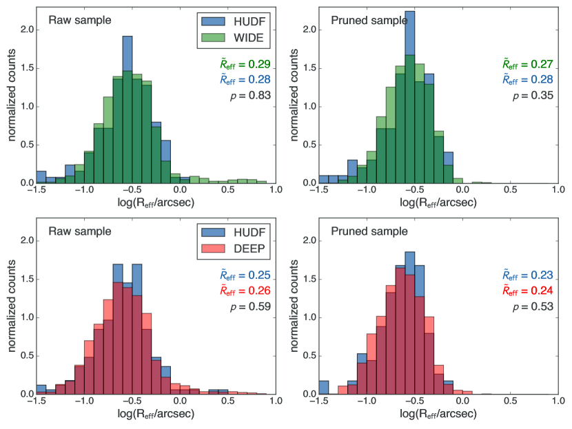
Figure 1: Histograms of effective radius $R_{\mathrm{eff}}$ for galaxies in narrow magnitude ranges in the Wide, Deep, and HUDF regions of our sample. The top panels compare the distributions of $R_{\mathrm{eff}}$ in the Wide and HUDF regions in the magnitude range $23.5$ mag $<H_{160}<24.5$ mag, while the bottom panels compare the distributions of $R_{\mathrm{eff}}$ in the Deep and HUDF regions in the magnitude range $24.2$ mag $<H_{160}<25.2$ mag. For reference, the selection limits of our sample in these regions are $H_{160}=24.5$ (Wide), 25.2 (Deep), and 26.7 mag (HUDF). The left and right panels compare the distributions before and after the sample pruning described in Section 2. The legends in the panels list the median values of $R_{\mathrm{eff}}$ in the four histograms, and the Kolmogorov-Smirnov probabilities that the histograms are drawn from the same underlying distribution. The consistency of the histograms in regions with different depths, before and after pruning, indicates that the distribution of galactic sizes in our sample is unbiased even near the selection limits.

Studying galaxy size evolution demands that we compare $R_{\mathrm{eff}}$ values at a similar rest-frame wavelength across redshift bins, so that we can eliminate the contributions from dust or stellar age gradient to the observed size evolution. We follow the procedure in van der Wel et al. (2014) to correct for galaxy color gradients and place galaxy sizes on the same rest-frame wavelength. To do this, we use galaxy sizes measured in $H_{160}$ for galaxies at $z>1.5$ and use the sizes measured in $J_{125}$ at $z<1.5$. Color gradients that lead to different galaxy sizes at different wavelengths are accounted for by a correction factor that is a function of galaxy redshift, stellar mass, and galaxy type (late-type or early-type). As the result of this color gradient correction, the measurements are converted into the $R_{\mathrm{eff}}$ near rest-frame 5000Å. The size correction is typically only a few percent, but it does reach $\sim$60% in some cases. For more details about the color gradient correction, we refer the readers to van der Wel et al. (2014), Section 2.2, and their equations (1) and (2).

Stellar masses and star formation rates are estimated by comparing our photometry with model SEDs, adopting a Chabrier (2003) initial mass function (IMF). Here the stellar masses of galaxies include all luminous stars and dark remnants at the time of observation (but not stellar ejecta). This method of estimating stellar masses has been extensively tested in Mobasher et al. (2015), and they found that typical stellar mass uncertainties are $\sim 0.25$ dex for the magnitude limits adopted here. The primary sources of systematic uncertainties are IMF and stellar evolution models; for galaxies with strong nebular emission lines, systematic uncertainties for stellar mass can be up to $\sim 0.4$ dex.

We restrict this study to galaxies with stellar masses $M_{*}>10^{7}\,M_{\odot}$. Above this limit, we include all galaxies brighter than the magnitude limits mentioned above, where we are confident that our measurements are robust and unaffected by size-dependent biases. For each redshift interval, we estimate the typical stellar mass of the faintest galaxies $M_{*,\rm{low}}$ by taking the median SED-fitted stellar mass estimate of galaxies within 0.1 mag of the HUDF magnitude limit. The values of $M_{*,\rm{low}}$ are listed in Table 1 and shown as thick tick marks at the bottoms of Figures 4–4. SED-based star formation rates can be uncertain by $\sim 0.4$ dex (Salmon et al., 2015); therefore, the uncertainties in the specific star formation rates (sSFRs) are roughly $\lesssim 0.6$ dex for our galaxy sample. In this paper, we select subsamples in the upper and lower 20% tails of the sSFR distribution. Because we are making a differential comparison between the relatively large populations in these tails, our results are not sensitive to the sSFR uncertainties.

3 Abundance Matching

In this study, we employ the technique of abundance matching to estimate the mass and hence the size of the dark matter halo associated with each galaxy in our sample. In essence, this technique compares the measured sizes of observed galaxies with the inferred sizes of matched halos in cosmological dark matter simulations. The basic assumption is that the rank ordering of galaxy (stellar) masses $M_{*}$ reflects on average the rank ordering of halo (virial) masses $M_{200c}$, i.e., that the cumulative number densities of galaxy masses and halo masses are equal: $n_{g}(>M_{*})=n_{h}(>M_{200c})$. This ansatz leads directly to a correspondence between $M_{*}$ and $M_{200c}$ known as the stellar mass–halo mass relation. While the assumption that galaxy masses and halo masses follow the same rank ordering is a reasonable approximation for statistical studies based on large samples such as ours, it cannot be exactly true for individual galaxies, which experience stochastic events such as mergers and starbursts throughout their histories.

Given an SMHM relation, we compute the halo mass $M_{200c}$ of each galaxy in our sample from its stellar mass $M_{*}$. We then compute the virial halo radius $R_{200c}$ using the standard formula

$$R_{200c}=\left[\frac{3M_{200c}}{4\pi\cdot 200\rho_{\rm{crit}}(z)}\right]^{1/3},$$ (1)

where $\rho_{\rm{crit}}(z)$ is the critical density of the universe at redshift $z$. In order to assess how sensitive our results are to the choice of SMHM relation, we perform all of our calculations with four different SMHM relations. All of these SMHM relations are based on the Chabrier (2003) stellar IMF and the same halo mass definition ${M_{200c}}$. They are plotted in Figures 2, 3, and 4 and discussed below.

SMHM relation 1. We have derived this new SMHM relation specifically for this study so that it is as consistent as possible with the CANDELS data set, selection criteria, and SED fitting procedure for our sample of galaxies with size measurements. In particular, we combine the stellar mass function $n_{g}(>M_{*})$ from Tomczak et al. (2014) with our determination of the halo mass function $n_{h}(>M_{200c})$ from the Millennium-II simulation (Boylan-Kolchin et al., 2009).

Tomczak et al. (2014) derived the stellar mass function of galaxies at $0.2<z<3$ in three of the five CANDELS fields, using selection criteria and procedures for estimating stellar masses similar to those for our sample, as described in Section 2. We have compared our stellar masses with those derived by Tomczak et al. (2014) and find no systematic offset and only a small scatter ($\sim 0.1$ dex). Tomczak et al. fitted a double Schechter function to the observed stellar mass function in differential form $dn_{g}(>M_{*})/dM_{*}$ in each of eight redshift bins. We adopt the Tomczak et al. results directly for the three bins of width $\Delta z=0.5$ covering the range $1.5<z<3.0$. However, for simplicity, we combine their results for the four bins of width $\Delta z=0.25$ covering the range $0.5<z<1.5$ into two bins of width $\Delta z=0.5$. In this step, we weight the observed comoving densities of galaxies by the comoving volume in each $\Delta z=0.25$ bin and then fit a double Schechter function to the combined comoving densities in each $\Delta z=0.5$ bin. For our lowest redshift bin, $0<z<0.5$, we adopt the Tomczak et al. stellar mass function in their lowest redshift bin, $0.2<z<0.5$, because it agrees well with the one at $<z>=0.1$ derived by Moustakas et al. (2013). Finally, we have derived the halo mass function $n_{h}(>M_{200c})$ from the Millennium-II simulation (Boylan-Kolchin et al., 2009) at the snapshot closest to the middle of each redshift bin and then matched this to the stellar mass function as described above to obtain the SMHM relation.

As a check on this procedure, we have independently derived our own stellar mass function from scratch by the $1/V_{\rm{max}}$ method for the galaxies in all five CANDELS fields in the six $\Delta z=0.5$ bins (albeit with approximate $K$-corrections in our estimates of $V_{\rm{max}}$). The resulting stellar mass function is nearly identical to the rebinned one from Tomczak et al. (2014). This adds to our confidence in the validity of SMHM relation 1, which we regard as the primary SMHM relation in this study.

Because our galaxy sample covers a wider range in stellar mass than the Tomczak et al. sample, we linearly extrapolate the SMHM relation in log–log space to both lower and higher masses. The solid lines in Figure 2 show the SMHM relation derived directly from the Tomczak et al. data, while the dashed lines show the extrapolated parts of the SMHM relation.

SMHM relation 2. Behroozi et al. (2013) derived this SMHM relation from published stellar mass and halo mass functions over a wide range of redshifts ($0<z<8$). This is probably the most prevalent SMHM relation in the literature. However, since it is based on stellar mass functions that are quite different from those derived using CANDELS data, it is not ideal for the present study. We use it mainly to gauge the sensitivity of our results to different SMHM relations. For consistency, we convert their halo mass $M_{\rm{vir}}$, defined using a redshift-dependent overdensity factor $\Delta_{\rm{vir}}(z)$ (Bryan & Norman, 1998), to our halo mass definition $M_{200c}$. The conversion assumes an NFW halo mass profile and the halo mass–concentration model calibrated in Diemer & Kravtsov (2015). The corrections are very small in general ($<0.1$ dex).

SMHM relation 3. This is the same SMHM relation adopted by Kravtsov (2013). He derived his own SMHM relation out of concerns that previous relations used stellar mass functions that are biased at both the high-mass and low-mass ends. By using the same SMHM relation as Kravtsov (2013), we can directly compare our galaxy size–halo size relation with his at $z=0$.

SMHM relation 4. There are several SMHM relations separated by galaxy type at $z<0.5$ in the literature, which we plot in Figure 3. These relations use different approaches to deriving the ratio between stellar masses and halo masses, ranging from abundance matching (Rodríguez-Puebla et al., 2015) to weak lensing (Hudson et al., 2015; Mandelbaum et al., 2016) to a mixture of the two methods (Dutton et al., 2010). We adopt the SMHM relation from Rodríguez-Puebla et al. (2015) because it has the largest dynamic range in halo mass and is in the middle of the range spanned by the other type-dependent relations from the literature. We use the Rodríguez-Puebla et al. SMHM relations for blue and red central galaxies at $z=0$ for galaxies in our sample with Sérsic index $n$ below and above 2.5, respectively. Since Rodríguez-Puebla et al. defined their halo mass using $\Delta_{\rm{vir}}(z)$, we have applied the same conversion to $M_{200c}$ as we did for SMHM relation 2.

We compare the four SMHM relations in Figure 4. Evidently, there are significant discrepancies among these SMHM relations, especially the first and second, for which the differences can be up to $\sim 0.5$ dex at $z\sim 3$. Our SMHM relation 1, derived specifically for the CANDELS sample at $0<z<3$, shows stronger redshift evolution than SMHM relation 2 from Behroozi et al. (2013). As already noted, this difference comes mainly from the different stellar mass functions used as input to these SMHM relations. Fortunately, as we show in Sections 4 and 5, our main scientific results are relatively insensitive to the adopted SMHM relation, largely due to the weak dependence of halo size on halo mass ($R_{200c}\propto M_{200c}^{1/3}$).

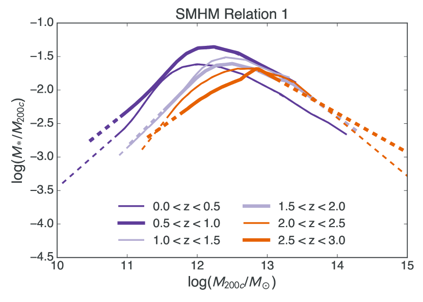
Figure 2: Ratio of galaxy stellar mass $M_{*}$ to halo virial mass $M_{200c}$ plotted against $M_{200c}$ for our primary SMHM relation in six redshift bins covering the range $0<z<3$. We derived this SMHM relation by abundance matching from an evolving stellar mass function appropriate for the CANDELS sample (Tomczak et al., 2014) and the evolving halo mass function in the Millennium-II simulation (Boylan-Kolchin et al., 2009) as described in Section 3. Solid lines are based directly on the stellar mass function from Tomczak et al. (2014); we linearly extrapolate the SMHM relation in log–log space to cover the stellar mass range of our sample (dashed lines).

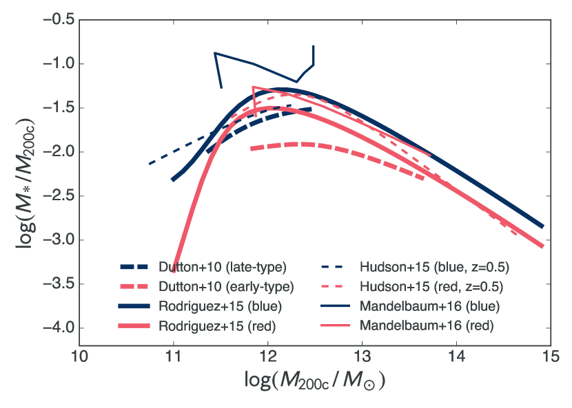
Figure 3: Ratio of galaxy stellar mass $M_{*}$ to halo virial mass $M_{200c}$ plotted against $M_{200c}$ for four low-redshift SMHM relations from the literature that depend on galaxy color or type. These were derived by abundance matching (Rodríguez-Puebla et al., 2015), weak lensing (Hudson et al., 2015; Mandelbaum et al., 2016), or a combination of both techniques (Dutton et al., 2010). Three of the SMHM relations pertain to $z=0$ and one to $z=0.5$ (Hudson et al., 2015). Note the large discrepancies among these color- and type-dependent SMHM relations.

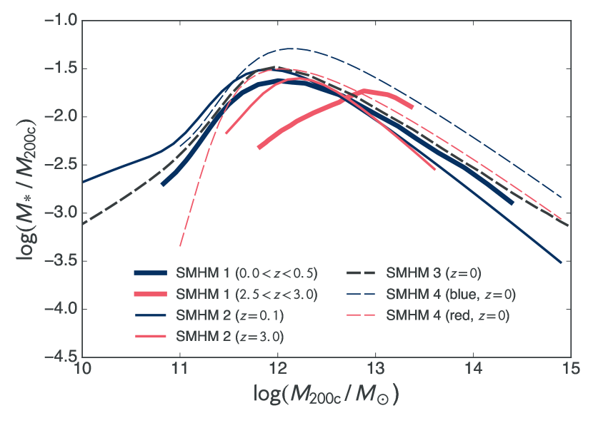
Figure 4: Ratio of galaxy stellar mass $M_{*}$ to halo virial mass $M_{200c}$ plotted against $M_{200c}$ for the four SMHM relations adopted in this work. SMHM relation 1: derived as described in Section 3 for all galaxies at $0<z<3$ and displayed here at $0<z<0.5$ and $2.5<z<3.0$, which bracket the relation at intermediate redshifts. SMHM relation 2: derived by Behroozi et al. (2013) for all galaxies at $0<z<8$ and displayed here at $z=0.1$ and $z=3.0$. SMHM relation 3: derived by Kravtsov (2013) for all galaxies only at $z=0$. SMHM relation 4: derived by Rodríguez-Puebla et al. (2015) separately for blue and red galaxies only at $z=0$. Note that there are significant differences among these SMHM relations, but because halo size depends weakly on halo mass ($R_{200c}\propto M_{200c}^{1/3}$), our main results are not sensitive to these differences.

4 Results

The main results of this paper are displayed in Figures 4–4 and described in this section. The uncertainties in these results, mostly stemming from the SMHM relation and morphological classification, are discussed in Section 5.

Our first main result is that galaxy sizes are proportional to halo sizes over a wide range of size and mass. Figure 4 shows galaxy $R_{\mathrm{eff}}$ plotted against halo $R_{200c}$ at $0<z<0.5$ for the four different SMHM relations. In each panel, the medians of $\log R_{\mathrm{eff}}$ in bins of width $\Delta\log R_{200c}=0.15$ dex are plotted as pentagons, and the 16th–84th percentile ranges as vertical bars; only the bins with more than five galaxies are shown. The halo radius limit corresponding to the reference stellar mass $M_{*,\rm{low}}$ from Table 1 is shown as a thick tick mark at the bottom of each panel. The coefficient of proportionality $\alpha$ in the relation $R_{\mathrm{eff}}=\alpha R_{200c}$ is nearly the same in all four cases; the median values of $\alpha$ are 0.021, 0.025, 0.023, and 0.024 for SMHM relations 1–4, respectively. These $R_{\mathrm{eff}}$–$R_{200c}$ relations are approximately linear, but with some subtle differences depending on the adopted SMHM relation.

Kravtsov (2013) also found a linear relation, using completely independent samples of galaxies at $z=0$ and de-projected 3D half-mass radii $R_{1/2}$ rather than the projected 2D half-light radii $R_{\mathrm{eff}}$. The solid line in Figure 4 shows his derived relation $R_{1/2}=\alpha^{\prime}R_{200c}$ with $\alpha^{\prime}=0.015$, assuming $R_{\mathrm{eff}}=R_{1/2}$ for pure-disk galaxies. The bulk of our sample by number lies above this relation by ${\sim 0.2}$ dex, agreeing better at the high- and low-mass ends. There are a number of possible explanations for this offset, one of them being the difference between 2D half-light (effective) and 2D half-mass radii. Szomoru et al. (2013) noted that for the galaxies more massive than $5\times 10^{10}~{}M_{\odot}$ at $0<z<2.5$, rest-frame $g$-band 2D half-light radii are on average $\sim$25% larger than 2D half-mass radii (presumably due to the influence of bulges), which could account for $\sim 0.1$ dex of the offset. We will address other explanations below in connection with morphological types, deprojection effects, and the redshift evolution.

Our second main result is that the $R_{\mathrm{eff}}$–$R_{200c}$ relations are offset for late-type and early-type galaxies. To separate morphological types, we split our sample in two different ways: (1) high-$n$ (early-type) and low-$n$ (late-type) subsamples, and (2) low-sSFR (early-type) and high-sSFR (late-type) subsamples. We only include the highest and lowest 20% of the sample in either $n$ or sSFR in the hope that this procedure will isolate disk-dominated from spheroid-dominated galaxies. The resulting $R_{\mathrm{eff}}$–$R_{200c}$ relations for late- and early-type galaxies using all four SMHM relations are shown in Figures 4 and 4.

We see in both Figures 4 and 4 that galaxies of different types follow sequences roughly parallel to the $R_{\mathrm{eff}}\propto R_{200c}$ line with an offset of $\sim 0.2$ dex at $0<z<0.5$. This result is relatively robust against SMHM relation and morphological classification method: early-type (high-$n$ or low-sSFR) galaxies have smaller $R_{\mathrm{eff}}$ than late-type (low-$n$ or high-sSFR) galaxies at the same halo masses. The effect persists even if we compare 3D half-light radii rather than 2D half-light radii $R_{\mathrm{eff}}$, although with a smaller separation between the sequences. The parallel sequences of early- and late-type galaxies in the $R_{\mathrm{eff}}$–$R_{200c}$ diagram are reminiscent of the parallel sequences of spheroid- and disk-dominated galaxies in the $J/M$ vs. $M$ diagram (Fall, 1983; Romanowsky & Fall, 2012; Fall & Romanowsky, 2013). The latter is due to a combination of different sizes (by a factor of $\sim$2) and different rotation velocities (also by a factor of $\sim$2–3) of spheroid- and disk-dominated galaxies of the same stellar mass.

This helps explain why our overall relation in Figure 4 is higher than Kravtsov’s at intermediate masses. Our sample is dominated by late-type galaxies ($\sim$90% have $n<2.5$), while Kravtsov’s sample is dominated by early-type galaxies ($\sim 80\%$ by number). He noted that late-type galaxies are systematically larger in $R_{1/2}$ than early-type galaxies at intermediate stellar masses, which is where we see the largest offset between these sequences in Figure 4. The changing morphological mix as a function of mass also helps explain the apparent curvature of the overall relation in Figure 4, because early-type galaxies dominate the high- and low-mass ends of the relation.

Our third main result is that the $R_{\mathrm{eff}}$–$R_{200c}$ relation for late-type galaxies is close to the predictions of the simple analytic model of disk formation. The scale radius and effective radius of an exponential disk embedded in a dark matter halo with a virial (outer) radius $R_{200c}$ and a spin parameter $\lambda$ are given by

$$R_{d}=\frac{\lambda}{\sqrt{2}}R_{200c}$$ (2)

and

$$R_{\mathrm{eff}}=1.68~{}R_{d},$$ (3)

when the disk and halo have the same specific angular momentum ($J/M$). Equation (2) is exact for isothermal halos (Fall & Efstathiou, 1980; see their Figure 3 and equation 42; Fall, 1983, see his equation 4) and is approximate for NFW halos with typical concentrations (Mo et al., 1998; Burkert et al., 2016). This prediction is shown as the dashed lines in Figures 4 to 4 for $\lambda=0.035$, the peak of the universal spin parameter distribution (Bullock et al., 2001; Bett et al., 2007). We find that late-type galaxies at $0<z<0.5$ lie $\sim 0.2$ dex below the $J/M$ equality line; in other words, our late-type galaxies have slightly less specific angular momentum than their dark matter halos. This offset is consistent with direct measurements of specific angular momentum at $z=0$, which indicate $J/M$ retention factors $\eta_{j}\sim 80\%\pm 20\%$ for galactic disks (Fall & Romanowsky, 2013).

Galaxy effective radius $R_{\mathrm{eff}}$ plotted against halo virial radius $R_{200c}$ in the lowest redshift interval ($0<z<0.5$) for the full sample of galaxies. The four panels show results for SMHM relations 1, 2, 3, and 4 as indicated. The faint gray dots represent individual galaxies, while the filled pentagons and vertical bars indicate the median values and 16th–84th percentile ranges of $R_{\mathrm{eff}}$ in bins of width 0.15 in $\log R_{200c}$. The diagonal lines show the $R_{1/2}$–$R_{200c}$ relation at $z=0$ from Kravtsov (2013) assuming $R_{\mathrm{eff}}=R_{1/2}$. The thick tick mark at the bottom of each panel indicates the halo size corresponding to the reference stellar mass $M_{*,\rm{low}}$ listed in Table 1. Note that the $R_{\mathrm{eff}}$–$R_{200c}$ relations are similar for the four different SMHM relations and are roughly consistent with Kravtsov’s results. The $R_{\mathrm{eff}}$–$R_{200c}$ relations are linear in a first approximation but exhibit some curvature at high and low masses as a result of the changing mix of galaxy morphologies. Compare with Figures 4 and 4.

Galaxy effective radius $R_{\mathrm{eff}}$ plotted against halo virial radius $R_{200c}$ in the lowest redshift interval ($0<z<0.5$) for subsamples of galaxies with the lowest and highest 20% of the measured Sérsic index $n$ as proxies for late- and early-type galaxies, respectively. The four panels show results for SMHM relations 1, 2, 3, and 4 as indicated. The faint blue and red dots represent individual low-$n$ and high-$n$ galaxies, respectively, while the filled blue squares, open red circles, and vertical bars indicate the corresponding median values and 16th–84th percentile ranges of $R_{\mathrm{eff}}$ in bins of width 0.15 in $\log R_{200c}$. The diagonal solid lines show the $R_{1/2}$–$R_{200c}$ relation at $z=0$ from Kravtsov (2013) assuming $R_{\mathrm{eff}}=R_{1/2}$, while the diagonal dashed lines show the prediction for galactic disks with the same $J/M$ as their surrounding halos. The thick tick mark at the bottom of each panel indicates the halo size corresponding to the reference stellar mass $M_{*,\rm{low}}$ listed in Table 1. Note that the $R_{\mathrm{eff}}$–$R_{200c}$ relation for low-$n$ galaxies is systematically above, and roughly parallel to, the relation for high-$n$ galaxies. The $R_{\mathrm{eff}}$–$R_{200c}$ relations for both subsamples of galaxies are more linear than the relations for the full sample. Compare with Figures 4 and 4.

Galaxy effective radius $R_{\mathrm{eff}}$ plotted against halo virial radius $R_{200c}$ in the lowest redshift interval ($0<z<0.5$) for subsamples of galaxies with the highest and lowest 20% of the measured sSFR as proxies for late- and early-type galaxies, respectively. The four panels show results for SMHM relations 1, 2, 3, and 4 as indicated. The faint blue and red dots represent individual high-sSFR and low-sSFR galaxies, respectively, while the filled blue squares, open red circles, and vertical bars indicate the corresponding median values and 16th–84th percentile ranges of $R_{\mathrm{eff}}$ in bins of width 0.15 in $\log R_{200c}$. The diagonal solid lines show the $R_{1/2}$–$R_{200c}$ relation at $z=0$ from Kravtsov (2013) assuming $R_{\mathrm{eff}}=R_{1/2}$, while the diagonal dashed lines show the prediction for galactic disks with the same $J/M$ as their surrounding halos. The thick tick mark at the bottom of each panel indicates the halo size corresponding to the reference stellar mass $M_{*,\rm{low}}$ listed in Table 1. Note that the $R_{\mathrm{eff}}$–$R_{200c}$ relation for high-sSFR galaxies is systematically above, and roughly parallel to, the relation for low-sSFR galaxies. The $R_{\mathrm{eff}}$–$R_{200c}$ relations for both subsamples of galaxies are more linear than the relations for the full sample. Compare with Figures 4 and 4.

Galaxy effective radius $R_{\mathrm{eff}}$ plotted against halo virial radius $R_{200c}$ at different redshifts for subsamples of galaxies with the lowest and highest 20% of the measured Sérsic index $n$ as proxies for late- and early-type galaxies, respectively. The six panels show results computed from SMHM relation 1 in redshift intervals of $\Delta z=0.5$ covering the range $0<z<3$. The faint blue and red dots represent individual low-$n$ and high-$n$ galaxies, respectively, while the filled blue squares, open red circles, and vertical bars indicate the corresponding median values and 16th–84th percentile ranges of $R_{\mathrm{eff}}$ in bins of width 0.15 in $\log R_{200c}$. The diagonal solid lines show the $R_{1/2}$–$R_{200c}$ relation at $z=0$ from Kravtsov (2013) assuming $R_{\mathrm{eff}}=R_{1/2}$, while the diagonal dashed lines show the prediction for galactic disks with the same $J/M$ as their surrounding halos. The thick tick mark at the bottom of each panel indicates the halo size corresponding to the reference stellar mass $M_{*,\rm{low}}$ listed in Table 1. Note that the $R_{\mathrm{eff}}$–$R_{200c}$ relations for both low-$n$ and high-$n$ galaxies are nearly constant with redshift, and that the one for low-$n$ galaxies is close to the predicted relation for equality of $J/M$ in disks and halos. Compare with Figure 4.

Galaxy effective radius $R_{\mathrm{eff}}$ plotted against halo virial radius $R_{200c}$ at different redshifts for subsamples of galaxies with the highest and lowest 20% of the measured sSFR as proxies for late- and early-type galaxies, respectively. The six panels show results computed from SMHM relation 1 in redshift intervals of $\Delta z=0.5$ covering the range $0<z<3$. The faint blue and red dots represent individual high-sSFR and low-sSFR galaxies, respectively, while the filled blue squares, open red circles, and vertical bars indicate the corresponding median values and 16th–84th percentile ranges of $R_{\mathrm{eff}}$ in bins of width 0.15 in $\log R_{200c}$. The diagonal solid lines show the $R_{1/2}$–$R_{200c}$ relation at $z=0$ from Kravtsov (2013) assuming $R_{\mathrm{eff}}=R_{1/2}$, while the diagonal dashed lines show the prediction for galactic disks with the same $J/M$ as their surrounding halos. The thick tick mark at the bottom of each panel indicates the halo size corresponding to the reference stellar mass $M_{*,\rm{low}}$ listed in Table 1. Note that the $R_{\mathrm{eff}}$–$R_{200c}$ relations for both high-sSFR and low-sSFR galaxies are nearly constant with redshift, and that the one for high-sSFR galaxies is close to the predicted relation for equality of $J/M$ in disks and halos. Compare with Figure 4.

Our fourth main result is that there is remarkably little evolution in the $R_{\mathrm{eff}}$–$R_{200c}$ relation from $z=3$ to $z=0$. This is shown in Figures 4 and 4. As in the previous diagrams, we select the highest and lowest 20% tails of the $n$ and sSFR distributions. We only show results for SMHM relation 1, but we have checked that they are similar for the other SMHM relations. Figures 4 and 4 show again that in all redshift bins, late-type galaxies follow a nearly linear relation: $R_{\mathrm{eff}}=\alpha R_{200c}$. At $0.5<z<3$, late-type galaxies have ${\alpha\approx 0.034}$ in Figure 4 (${\alpha\approx 0.029}$ in Figure 4) and lie close to the $J/M$ equality line (within $\lesssim$ 0.1–0.2 dex) with no discernible evolution. (There is a slight offset to smaller sizes in the late-type sample when selected by sSFR rather than Sérsic index.) This result agrees with recent direct measurements of specific angular momentum at $0.2<z<1.4$ (Contini et al., 2016) and at $1<z<3$ (Burkert et al., 2016), which show that $J/M$ in galactic disks is nearly the same as in their dark matter halos.

Kravtsov (2013) speculated that the sizes of galaxies grew in proportion to the sizes of their halos until $z\sim 2$ and then stopped, while their halos continued to grow in mass and size. We find instead that the $R_{\mathrm{eff}}$–$R_{200c}$ relations at $z<2$ are very similar to those at $z>2$. Our $R_{\mathrm{eff}}$–$R_{200c}$ relations for the late-type galaxies at $z<0.5$ have smaller amplitudes than those at $z>0.5$, indicating a possible slowdown in the growth of disks, but this deviation is mild ($\sim$0.2 dex) and not established beyond all doubt (see below).

The $R_{\mathrm{eff}}$–$R_{200c}$ relation for early-type galaxies is also nearly constant. We see in Figures 4 and 4 that the trend for early-type galaxies at all redshifts roughly parallels that for late-type galaxies, but shifted down by $\sim 0.2$ dex at $0<z<0.5$ and by $\sim$ 0.2–0.3 dex at $0.5<z<3$. There is a slight hint of a “turnover” at the most massive end at $0<z<0.5$ (see Figures 4 and 4). This turnover, if real, could be due to either size-measurement biases (due to diffuse outer halos surrounding central galaxies in groups and clusters) or the breakdown of abundance matching for the group- or cluster-mass halos.

5 Uncertainties

How robust are these results? The uncertainties in this study potentially include measurement and statistical errors internal to the CANDELS data set, as well as external systematic errors from the adopted SMHM relations and stellar population models. Here we provide a brief assessment of these uncertainties.

As noted in Section 2, errors in the measurements of effective radii $R_{\mathrm{eff}}$ (from fits to Sérsic profiles) are relatively small: $<20\%$ (systematic) to $30\%$ (random). Even if these errors were at the upper end of this range for all galaxies and varied systematically with galactic masses and sizes, they would have a negligible influence on the coefficient and exponent of the galaxy size–halo size relation: $R_{\mathrm{eff}}=\alpha R_{200c}^{\beta}$ with $|\Delta\alpha/\alpha|\lesssim 0.02$ and $|\Delta\beta|\lesssim 0.08$ (assuming a $\sim 20\%$ or smaller systematic deviation in $R_{\mathrm{eff}}$ for a factor of 10 or more variation in $R_{200c}$). Because the sample size in this study is so large ($N\sim 38000$), the effects of random errors in the size measurements on the mean $R_{\mathrm{eff}}$–$R_{200c}$ relations are even smaller. In a situation like this, with negligible internal errors, formal tests of goodness of fit are not informative, and we do not attempt them.

The dominant uncertainties in our galaxy size–halo size relations are most likely caused by possible systematic errors in our adopted SMHM relations. We can judge the magnitude of these errors by comparing the $R_{\mathrm{eff}}$–$R_{200c}$ relations plotted in Figures 4 to 4 for the four different SMHM relations. This comparison indicates that the SMHM relation may be responsible for systematic errors at the level of $\sim 0.1$–$0.2$ dex, perhaps a little less for the combined sample of galaxies, perhaps a little more for the subsamples split by morphological type. Quantitative measures of the deviations among the $R_{\mathrm{eff}}$–$R_{200c}$ relations at $0<z<0.5$ confirm these impressions.

The contributions to the error budget from the adopted stellar population models, which determine the stellar masses and specific star formation rates, are smaller than those from the adopted SMHM relations. Systematic errors in stellar masses could affect the $R_{\mathrm{eff}}$–$R_{200c}$ relations at about the same level as systematic errors in $R_{\mathrm{eff}}$. The classification of the 3D shapes of galaxies (i.e., flat disks vs. round spheroids) by Sérsic index is another source of uncertainty, because it is based only on the radial decline of the projected 2D surface brightness profiles. Fitting a single Sérsic profile instead of a detailed disk/bulge decomposition possibly adds further uncertainty. Nevertheless, the $R_{\mathrm{eff}}$–$R_{200c}$ relations we obtain from subsamples split by Sérsic index agree at the $\lesssim 0.1$ dex level with those from subsamples split by specific star formation rate.

We estimate the impact of selection biases on our galaxy size–halo size relations from the detection efficiencies for the CANDELS survey derived by Guo et al. (2013) as follows. They divide the $R_{\mathrm{eff}}$–$H_{160}$ plane into regions that are 0–50%, 50–90%, and 90–100% complete. Most of our sample (88%) lies in the region of 90–100% completeness, while the remainder (12%) lies in the region of 50–90% completeness. To place an upper limit on the impact of selection biases, we adopt the lower limits of 90% and 50% on the completeness in these two regions of the $R_{\mathrm{eff}}$–$H_{160}$ plane, assign weights 2.0 (i.e., $1/0.5$) and 1.1 (i.e., $1/0.9$) to the galaxies in our sample in these regions, and then recompute the $R_{\mathrm{eff}}$–$R_{200c}$ relations. For $R_{200c}\gtrsim 100$ kpc, we find negligible corrections to the median $R_{\mathrm{eff}}$–$R_{200c}$ relations, while for $R_{200c}\lesssim 100$ kpc, we find corrections below 0.1 dex for all galaxy types and redshifts $0<z<3$. We conclude from this exercise that selection biases are likely to be subdominant sources of uncertainty in our $R_{\mathrm{eff}}$–$R_{200c}$ relations.

Based on this assessment of uncertainties, most of the results of this paper appear to be robust. In particular, there is a strong, approximately linear correlation between the sizes of galaxies and their dark matter halos over the full range of redshifts examined here, $0<z<3$. The coefficient of proportionality is larger for late-type galaxies than for early-type galaxies, which follow roughly parallel sequences, except possibly at the highest redshifts. For late-type galaxies, the observed $R_{\mathrm{eff}}$–$R_{200c}$ relation is generally consistent with simple models in which galactic disks grow with the same specific angular momentum as their dark matter halos. There is some evidence for a slowdown in disk growth at $z<0.5$, but the apparent deviation from the $J/M$ equality line is only $\sim 0.2$ dex.

Table 2: Verification of Main Results

	SMHM 1	SMHM 2	SMHM 3	SMHM 4
1. The $R_{\mathrm{eff}}$–$R_{200c}$ relations are roughly linear in all redshift bins.	T	T	T	T
2. The $R_{\mathrm{eff}}$–$R_{200c}$ relations are offset for early- and late-type galaxies.	T	T	T	T
3. The $R_{\mathrm{eff}}$–$R_{200c}$ relation for late-type galaxies are close to the $J/M$ equality line.	T	T	T	T
4. The $R_{\mathrm{eff}}$–$R_{200c}$ relation shows little evolution between $z=0$ and $z=3$.	T	T	T	T

We have plotted and examined the $R_{\mathrm{eff}}$–$R_{200c}$ relations at all redshifts ($0<z<3$) for all four SMHM relations to determine whether or not they support the four main results discussed in Section 4. The outcome of this test is recorded in Table 2 by a T (for true) or F (for false) for each combination of SMHM relation and result. All of the entries are Ts. Table 2 therefore reinforces our conclusion that the main scientific results of this study are robust relative to discrepancies among the SMHM relations (because of the weak dependence of $R_{200c}$ on $M_{200c}$).

6 Discussion

We have found that the sizes of galaxies are proportional on average to the sizes of their dark matter halos over a wide range of galaxy and halo masses and over the entire redshift range $0<z<3$ studied here: $R_{\mathrm{eff}}=\alpha R_{200c}$ with $\alpha\approx 0.03$. In particular, we confirm the basic relation found by Kravtsov (2013) at $z=0$ with only minor adjustment, some of which is related to the difference between 2D half-light radii and 3D half-mass radii. There is some curvature at the upper end of our overall $R_{\mathrm{eff}}$–$R_{200c}$ relation, which is due to the larger abundance and smaller average size of early-type galaxies compared with late-type galaxies of the same stellar mass. Indeed, we find that early- and late-type galaxies follow distinct, roughly parallel $R_{\mathrm{eff}}$–$R_{200c}$ relations offset by a factor of $\sim 2$ for the upper and lower 20th percentiles of Sérsic index and specific star formation rate, which are meant to be proxies for disk-dominated and spheroid-dominated galaxies.

Given the proportionality between galaxy and halo sizes, it is now straightforward to predict how galaxy sizes evolve with redshift, from the following alternative forms of equation (1):

$$R_{\mathrm{eff}}=\alpha R_{200c}=\alpha\left[\frac{GM_{200c}}{100H^{2}(z)}\right]^{1/3}=\alpha\frac{{V_{200c}}}{10H(z)}.$$ (4)

Here $H(z)$ is the Hubble parameter at redshift $z$, and ${V_{200c}}$ is the circular velocity of the halo in question (see Mo et al., 1998). Thus, we expect $R_{\mathrm{eff}}\propto{H^{-2/3}(z)}$ or $R_{\mathrm{eff}}\propto{H^{-1}(z)}$ depending on whether galaxies at different $z$ are compared at the same $M_{200c}$ or ${V_{200c}}$. As a result of gravitational clustering, the characteristic halo mass evolves with redshift roughly as $\sigma({M^{*}_{200c}},z)\propto\delta_{c}(z)/D(z)$, where $\sigma({M^{*}_{200c}},z)$ is the RMS deviation of the linear density field smoothed over the scale ${R(M^{*}_{200c})}$, $\delta_{c}(z)$ is the critical linear overdensity for collapse (Kitayama & Suto, 1996), and $D(z)$ is the linear growth factor (Carroll et al., 1992). The corresponding galactic size $R_{\mathrm{eff}}^{*}(z)$ at the knee of the galaxy mass function should evolve according to equation (4) with $M_{200c}\rightarrow{M^{*}_{200c}}(z)$. This expression for $R_{\mathrm{eff}}^{*}(z)$ relates the typical sizes of progenitor–descendant pairs of galaxies at different redshifts, although there will be a large dispersion about it as a result of stochasticity in the hierarchical growth of galaxies.

Our $R_{\mathrm{eff}}$–$R_{200c}$ relations for late-type galaxies (defined by low $n$, high sSFR) at $0.5<z<3$ are within $\lesssim$ 0.1–0.2 dex of the predictions of simple models in which galactic disks acquire and retain the same specific angular momentum as induced by tidal torques in their surrounding dark matter halos. At $z<0.5$, late-type galaxies are $\sim 0.2$ dex below this prediction. However, given possible systematic errors in the measurements of galactic sizes ($\lesssim 20\%$ for low-$n$ galaxies), our results are consistent with a range $\eta_{j}\sim 80\%\pm 20\%$ for the retained fraction of specific angular momentum. Our results therefore agree nicely with recent, direct measurements of the specific angular momentum of galactic disks at $z=0$ (Fall & Romanowsky, 2013), at $0.2<z<1.4$ (Contini et al., 2016), and at $1<z<3$ (Burkert et al., 2016), all of which indicate retention factors $\eta_{j}$ near unity or slightly below.

The notion of angular momentum conservation was introduced as a simplifying approximation in the era of analytical models of galaxy formation (Fall & Efstathiou, 1980). Since then, hydrodynamical models have revealed a much more complex situation. In particular, it is now clear that several physical processes may change the specific angular momentum of galaxies or parts of galaxies during their formation and evolution, including merging, feedback, inflows, outflows, and gravitational interactions between baryons and dark matter. Some of these processes cause gains in specific angular momentum, while others cause losses (see Romanowsky & Fall 2012 and Genel et al. 2015 for summaries and references to earlier work).

The galactic disks that form in recent hydrodynamical simulations have nearly the same specific angular momentum on average as their dark matter halos, in good agreement with observations (Genel et al., 2015; Pedrosa & Tissera, 2015; Teklu et al., 2015; Zavala et al., 2016). Evidently, the processes responsible for gains and losses are either weak or in rough balance, leading to an apparent (if not strict) conservation of angular momentum during the formation of galactic disks. Simulations and now observations indicate that galaxies of all types grow in a quasi-homologous (or self-similar) relationship with their dark matter halos. The details of how this happens are a topic of ongoing research.

We thank Gerard Lemson for the help with Millennium Simulation, Adam Tomczak for useful discussions of stellar mass functions, and Andrey Kravtsov for providing conversion factors between different halo mass definitions. We also thank Avishai Dekel, Sandra Faber, Steve Finkelstein, Andrey Kravtsov, Yu Lu, and Rachel Somerville for comments on a near-final draft of this paper. This work is based on observations taken by the CANDELS Multi-Cycle Treasury Program with the NASA/ESA HST, which is operated by the Association of Universities for Research in Astronomy, Inc., under NASA contract NAS5-26555.

Transformation Between the $R_{\mathrm{eff}}$–$M_{*}$ and $R_{\mathrm{eff}}$–$R_{200c}$ Relations

The halo virial radius $R_{200c}$ of each galaxy in our sample was computed by the abundance-matching technique, i.e., from its stellar mass $M_{*}$, the SMHM relation, and Equation (1). Thus, the positions of galaxies in the $R_{\mathrm{eff}}$–$R_{200c}$ plane represent a nonlinear transformation of their positions in the $R_{\mathrm{eff}}$–$M_{*}$ plane. While the former is more fundamental from a theoretical perspective and is the main focus of this paper, the latter is one step closer to the observations, since it requires only the conversion of luminosities and colors into stellar masses. It is therefore of interest to examine the $R_{\mathrm{eff}}$–$M_{*}$ diagrams for our sample and how they map into the $R_{\mathrm{eff}}$–$R_{200c}$ diagrams presented in Section 4. This is the purpose of this appendix.

Figure 10 shows the $R_{\mathrm{eff}}$–$M_{*}$ diagram for galaxies in our sample in six redshift intervals covering the range $0<z<3$ when divided, as before, into subsamples with the lowest and highest quintiles of Sérsic index $n$. We also plot in this diagram the median values of $R_{\mathrm{eff}}$ in bins of width 0.5 in $\log M_{*}$ for these two subsamples. Evidently, the median $R_{\mathrm{eff}}$–$M_{*}$ relation for low-$n$ galaxies is close to a single power law (a straight line in a plot of $\log R_{\mathrm{eff}}$ against $\log M_{*}$), whereas the relation for high-$n$ galaxies is more complicated: it is flatter than the low-$n$ relation at low masses and steeper at high masses, with a bend at $M_{*}\sim{\rm few}\times 10^{10}~{}M_{\odot}$. It is also clear from Figure 10 that the median $R_{\mathrm{eff}}$–$M_{*}$ relations for both low-$n$ and high-$n$ galaxies evolve very slowly. For subsamples with the highest and lowest quintiles of specific star formation rate, we find similar behaviors in the median $R_{\mathrm{eff}}$–$M_{*}$ relations, as functions of both $M_{*}$ and $z$, especially for $z<1.5$ (not shown here).

Figure 11 shows the result of transforming the $R_{\mathrm{eff}}$–$M_{*}$ diagram into the $R_{\mathrm{eff}}$–$R_{200c}$ diagram with SMHM relation 1. This is exactly the same as Figure 4 except that we have omitted the vertical bars for clarity. We have already discussed this diagram at length in Section 4. Here we note only that the median $R_{\mathrm{eff}}$–$R_{200c}$ relations for low-$n$ and high-$n$ galaxies in Figure 11 appear more parallel than the corresponding $R_{\mathrm{eff}}$–$M_{*}$ relations in Figure 10, particularly at $z<1.5$, where they are best defined. This is a consequence of the nonlinearity of the SMHM relation, especially near $M_{200c}\sim 10^{12}~{}M_{\odot}$, corresponding to $M_{*}\sim{\rm few}\times 10^{10}~{}M_{\odot}$, and hence near the bend in the $R_{\mathrm{eff}}$–$M_{*}$ relation for high-$n$ galaxies.

van der Wel et al. (2014) also derived $R_{\mathrm{eff}}$–$M_{*}$ relations in the redshift range $0<z<3$ for galaxies in the CANDELS sample. The main difference between their work and ours is that they adopted the same selection limits in all CANDELS regions, whereas we adopted fainter selection limits in the Deep and HUDF regions. As a result, our $R_{\mathrm{eff}}$–$M_{*}$ relations extend to much lower $M_{*}$ than theirs. Otherwise, the selection of galaxies and measurement of their properties are nearly identical in the two studies. van der Wel et al. (2014) divided their sample into blue and red galaxies on the basis of rest-frame $UVJ$ colors rather than by Sérsic index or specific star formation rate, as we have done. Naturally, there is a general, but not a perfect, correspondence between these three different proxies for late- and early-type galaxies.

van der Wel et al. (2014) fitted power laws to the $R_{\mathrm{eff}}$–$M_{*}$ relations for blue and red galaxies; these are shown in Figure 10 as the blue solid and red dashed line segments, respectively. For red galaxies, they truncated the fits at $M_{*}=2\times 10^{10}~{}M_{\odot}$ because they also noticed a bend in the $R_{\mathrm{eff}}$–$M_{*}$ relation near this mass and a flattening below it. We obtain nearly identical results when we divide our sample into blue and red galaxies using the same cuts in rest-frame $UVJ$ colors as van der Wel et al. (2014). The blue solid and red dashed curves in Figure 11 show how the van der Wel et al. (2014) power laws in the $R_{\mathrm{eff}}$–$M_{*}$ diagram transform into the $R_{\mathrm{eff}}$–$R_{200c}$ diagram. As expected, this mapping introduces curvature and makes the $R_{\mathrm{eff}}$–$R_{200c}$ relations for blue and red galaxies somewhat more parallel. However, the transformed relations cover only a narrow range of halo sizes, roughly $100~{}{\rm kpc}\lesssim R_{200c}\lesssim 300~{}{\rm kpc}$, except in the lowest redshift interval. We have been able to extend the $R_{\mathrm{eff}}$–$R_{200c}$ relations to a wider range of halo sizes, roughly ${50}~{}{\rm kpc}\lesssim R_{200c}\lesssim 300~{}{\rm kpc}$, with our fainter selection limits in the CANDELS Deep and HUDF regions.

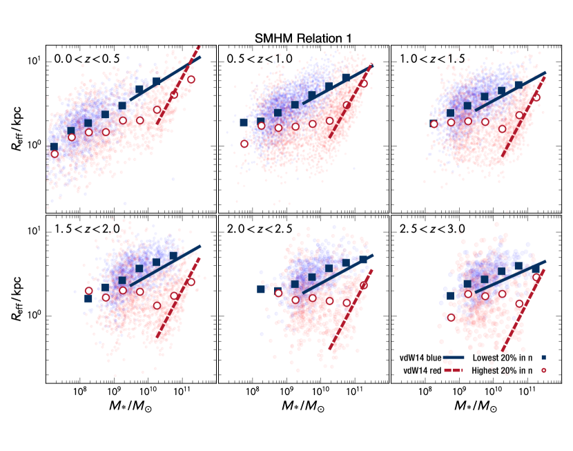
Figure 10: Galaxy effective radius $R_{\mathrm{eff}}$ plotted against stellar mass $M_{*}$ at different redshifts for subsamples of galaxies with the lowest and highest 20% of the measured Sérsic index $n$ as proxies for late- and early-type galaxies, respectively. The six panels show results computed from SMHM relation 1 in redshift intervals of $\Delta z=0.5$ covering the range $0<z<3$. The faint blue and red dots represent individual low-$n$ and high-$n$ galaxies, respectively, while the filled blue squares and open red circles indicate the corresponding median values of $R_{\mathrm{eff}}$ in bins of width 0.5 in $\log M_{*}$. The blue solid and red dashed lines show the power-law fits to the $R_{\mathrm{eff}}$–$M_{*}$ relations for blue and red galaxies (defined in terms of rest-frame $UVJ$ colors) from van der Wel et al. (2014). Note that our sample extends to fainter and therefore less massive galaxies than the van der Wel et al. (2014) sample. Compare with Figure 11.

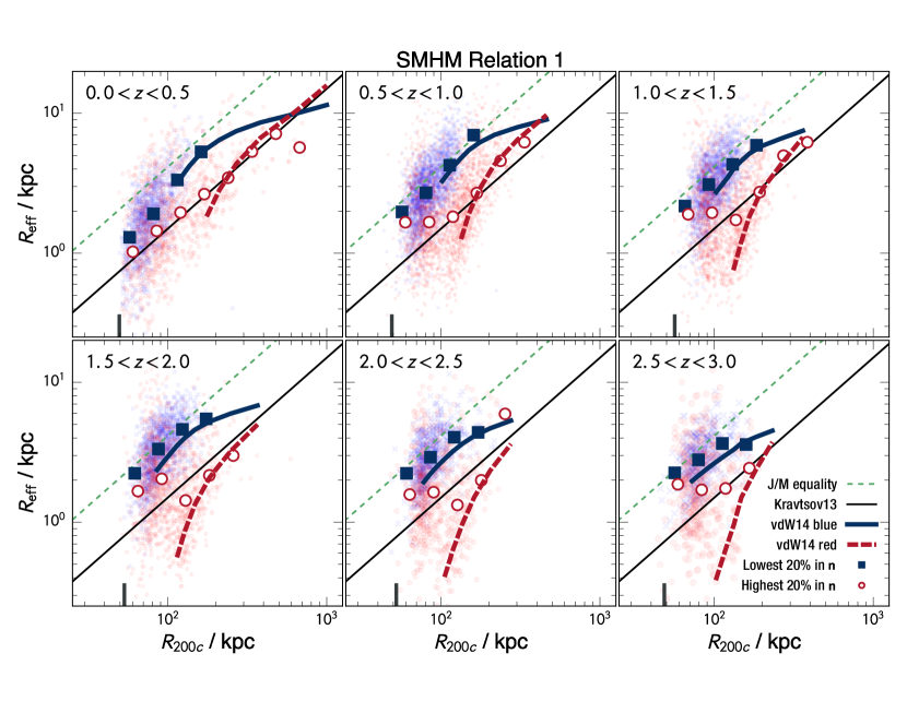
Figure 11: Galaxy effective radius $R_{\mathrm{eff}}$ plotted against halo virial radius $R_{200c}$ at different redshifts for subsamples of galaxies with the lowest and highest 20% of the measured Sérsic index $n$ as proxies for late- and early-type galaxies, respectively. The six panels show results computed from SMHM relation 1 in redshift intervals of $\Delta z=0.5$ covering the range $0<z<3$. The faint blue and red dots represent individual low-$n$ and high-$n$ galaxies, respectively, while the filled blue squares and open red circles indicate the corresponding median values of $R_{\mathrm{eff}}$ in bins of width 0.15 in $\log R_{200c}$. The diagonal solid lines show the $R_{1/2}$–$R_{200c}$ relation at $z=0$ from Kravtsov (2013) assuming $R_{\mathrm{eff}}=R_{1/2}$, while the diagonal dashed lines show the prediction for galactic disks with the same $J/M$ as their surrounding halos. The thick tick mark at the bottom of each panel indicates the halo mass corresponding to the reference stellar mass $M_{*,\rm{low}}$ listed in Table 1. The blue solid and red dashed curves are the power-law fits for blue and red galaxies in the $R_{\mathrm{eff}}$–$M_{*}$ plane after transformation into the $R_{\mathrm{eff}}$–$R_{200c}$ plane. Compare with Figure 10.

References

- Behroozi et al. (2013) Behroozi, P. S., Wechsler, R. H., & Conroy, C. 2013, ApJ, 770, 57
- Bertin & Arnouts (1996) Bertin, E., & Arnouts, S. 1996, A&AS, 117, 393
- Bett et al. (2007) Bett, P., Eke, V., Frenk, C. S., et al. 2007, MNRAS, 376, 215
- Boylan-Kolchin et al. (2009) Boylan-Kolchin, M., Springel, V., White, S. D. M., Jenkins, A., & Lemson, G. 2009, MNRAS, 398, 1150
- Bouwens et al. (2001) Bouwens, R., Illingworth, G. D., Oesch, P. A., et al. 2010, ApJ, 709, L133
- Bouwens et al. (2010) Bouwens, R. J., Illingworth, G. D., Oesch, P. A., et al. 2010, ApJ, 709, L133
- Bryan & Norman (1998) Bryan, G. L., & Norman, M. L. 1998, ApJ, 495, 80
- Bullock et al. (2001) Bullock, J. S., Dekel, A., Kolatt, T. S., et al. 2001, ApJ, 555, 240
- Burkert et al. (2016) Burkert, A., Förster Schreiber, N. M., Genzel, R., et al. 2016, ApJ, 826, 214
- Carroll et al. (1992) Carroll, S. M., Press, W. H., & Turner, E. L. 1992, ARA&A, 30, 499
- Chabrier (2003) Chabrier, G. 2003, PASP, 115, 763
- Cole et al. (2000) Cole, S., Lacey, C. G., Baugh, C. M., & Frenk, C. S. 2000, MNRAS, 319, 168
- Contini et al. (2016) Contini, T., Epinat, B., Bouché, N., et al. 2016, A&A, 591, A49
- Croton et al. (2016) Croton, D. J., Stevens, A. R. H., Tonini, C., et al. 2016, ApJS, 222, 22
- Curtis-Lake et al. (2016) Curtis-Lake, E., McLure, R. J., Dunlop, J. S., et al. 2016, MNRAS, 457, 440
- Diemer et al. (2013) Diemer, B., More, S., & Kravtsov, A. V. 2013, ApJ, 766, 25
- Diemer & Kravtsov (2015) Diemer, B., & Kravtsov, A. V. 2015, ApJ, 799, 108
- Dutton et al. (2010) Dutton, A. A., Conroy, C., van den Bosch, F. C., Prada, F., & More, S. 2010, MNRAS, 407, 2
- Ellis et al. (2013) Ellis, R. S., McLure, R. J., Dunlop, J. S., et al. 2013, ApJ, 763, L7
- Fall & Efstathiou (1980) Fall, S. M., & Efstathiou, G. 1980, MNRAS, 193, 189
- Fall (1983) Fall, S. M. 1983, in IAU Symp. 100, Internal Kinematics and Dynamics of Galaxies, ed. E. Athanassoula (Cambridge: Cambridge Univ. Press), 391
- Fall & Romanowsky (2013) Fall, S. M., & Romanowsky, A. J. 2013, ApJ, 769, L26
- Ferguson et al. (2004) Ferguson, H. C., Dickinson, M., Giavalisco, M., et al. 2004, ApJ, 600, L107
- Galametz et al. (2013) Galametz, A., Grazian, A., Fontana, A., et al. 2013, ApJS, 206, 10
- Genel et al. (2015) Genel, S., Fall, S. M., Hernquist, L., et al. 2015, ApJ, 804, L40
- Grogin et al. (2011) Grogin, N. A., Kocevski, D. D., Faber, S. M., et al. 2011, ApJS, 197, 35
- Guo et al. (2013) Guo, Y., Ferguson, H. C., Giavalisco, M., et al. 2013, ApJS, 207, 24
- Hathi et al. (2008) Hathi, N. P., Malhotra, S., & Rhoads, J. E. 2008, ApJ, 673, 686-693
- Huang et al. (2013) Huang, K.-H., Ferguson, H. C., Ravindranath, S., & Su, J. 2013, ApJ, 765, 68
- Hudson et al. (2015) Hudson, M. J., Gillis, B. R., Coupon, J., et al. 2015, MNRAS, 447, 298
- Illingworth et al. (2013) Illingworth, G. D., Magee, D., Oesch, P. A., et al. 2013, ApJS, 209, 6
- Kitayama & Suto (1996) Kitayama, T., & Suto, Y. 1996, ApJ, 469, 480
- Koekemoer et al. (2011) Koekemoer, A. M., Faber, S. M., Ferguson, H. C., et al. 2011, ApJS, 197, 36
- Koekemoer et al. (2013) Koekemoer, A. M., Ellis, R. S., McLure, R. J., et al. 2013, ApJS, 209, 3
- Kravtsov (2013) Kravtsov, A. V. 2013, ApJ, 764, L31
- Mandelbaum et al. (2016) Mandelbaum, R., Wang, W., Zu, Y., et al. 2016, MNRAS, 457, 3200
- Mo et al. (1998) Mo, H. J., Mao, S., & White, S. D. M. 1998, MNRAS, 295, 319
- Mobasher et al. (2015) Mobasher, B., Dahlen, T., Ferguson, H. C., et al. 2015, ApJ, 808, 101
- Moustakas et al. (2013) Moustakas, J., Coil, A. L., Aird, J., et al. 2013, ApJ, 767, 50
- Mosleh et al. (2012) Mosleh, M., Williams, R. J., Franx, M., et al. 2012, ApJ, 756, L12
- Nayyeri et al. (2016) Nayyeri, H., Hemmati, S., Mobasher, B., et al. 2016, arXiv:1612.07364
- Pedrosa & Tissera (2015) Pedrosa, S. E., & Tissera, P. B. 2015, A&A, 584, A43
- Peng et al. (2010) Peng, C. Y., Ho, L. C., Impey, C. D., & Rix, H.-W. 2010, AJ, 139, 2097
- Rodríguez-Puebla et al. (2015) Rodríguez-Puebla, A., Avila-Reese, V., Yang, X., et al. 2015, ApJ, 799, 130
- Romanowsky & Fall (2012) Romanowsky, A. J., & Fall, S. M. 2012, ApJS, 203, 17
- Salmon et al. (2015) Salmon, B., Papovich, C., Finkelstein, S. L., et al. 2015, ApJ, 799, 183
- Santini et al. (2015) Santini, P., Ferguson, H. C., Fontana, A., et al. 2015, ApJ, 801, 97
- Shibuya et al. (2015) Shibuya, T., Ouchi, M., & Harikane, Y. 2015, ApJS, 219, 15
- Straatman et al. (2016) Straatman, C. M. S., Spitler, L. R., Quadri, R. F., et al. 2016, ApJ, 830, 51
- Szomoru et al. (2013) Szomoru, D., Franx, M., van Dokkum, P. G., et al. 2013, ApJ, 763, 73
- Taghizadeh-Popp et al. (2015) Taghizadeh-Popp, M., Fall, S. M., White, R. L., & Szalay, A. S. 2015, ApJ, 801, 14
- Teklu et al. (2015) Teklu, A. F., Remus, R.-S., Dolag, K., et al. 2015, ApJ, 812, 29
- Tomczak et al. (2014) Tomczak, A. R., Quadri, R. F., Tran, K.-V. H., et al. 2014, ApJ, 783, 85
- van der Wel et al. (2012) van der Wel, A., Bell, E. F., Häussler, B., et al. 2012, ApJS, 203, 24
- van der Wel et al. (2014) van der Wel, A., Franx, M., van Dokkum, P. G., et al. 2014, ApJ, 788, 28
- Zavala et al. (2016) Zavala, J., Frenk, C. S., Bower, R., et al. 2016, MNRAS, 460, 4466