Mabuchi Solitons and Relative Ding Stability of Toric Fano Varieties

Abstract.

As a generalization of Kähler-Einstein metrics for Fano manifolds with nonvanishing Futaki invariant, Mabuchi solitons are critical points of a Calabi-type energy functional. We study their existence on toric Fano varieties and the underlying algebraic stability notion: relative Ding stability. As a toy model for a YTD type correspondence, a new feature is the emergence of a non-uniformly stable case. We show a partial coercivity for the modified Ding functionals in this case, and obtain singular Mabuchi solitons via a variational approach. In the unstable case, we determine the maximal destabilizer which is a simple convex function over the moment polytope, and establish a Moment-Weight equality which connects the infimum of a Calabi-type energy and the Berman-Ding invariant.

1. Introduction

For a polarized Kähler manifold $(X,L)$, a central problem is the existence of constant scalar curvature Kähler (cscK) metrics in class $c_{1}(L)$. The Yau-Tian-Donaldson conjecture predicts the existence is equivalent to K-polystability of $(X,L)$. In recent years, there are great progresses toward this conjecture, such as the confirmation for the Fano case, where $L=c_{1}(X)$ and cscK metrics are Kähler-Einstein (KE) metrics, see [CDS, T, BBJ], etc.

Recall that cscK metrics can be realized as zeros of the moment map in an infinitely dimensional GIT (geometric invariant theory) model discovered by Fujiki [Fuj] and Donaldson [D1]. The associated Kempf-Ness function is the Mabuchi functional (or K-energy) $M(\phi)$. K-stability was introduced by Tian (extended by Donaldson) as an analogue of Hilbert-Mumford’s criterion in GIT, via the limit slope of $M(\phi)$ along Bergman geodesics.

As a generalization of cscK metrics, the extremal metrics in $c_{1}(L)$ are defined as the critical points of the $L^{2}$-norm of the moment map

$$Cal(\omega)=\frac{1}{V}\int_{X}\left(S(\omega)-\bar{S}\right)^{2}\omega^{n},\ \omega\in c_{1}(L),\ V=[\omega]^{n},$$

called the Calabi energy, where $S(\omega)$ is the scalar curvature. Their existence is expected to be equivalent to relative K-stability, see [Sz2]. In [D4], Donaldson found a new GIT model specialized for Fano manifolds, where the moment map is

$$c_{1}(X)\ni\omega\longmapsto 1-e^{h_{\omega}},$$

where $h_{\omega}$ is the Ricci potential satisfying $Ric(\omega)-\omega=i\partial\bar{\partial}h_{\omega}$ and $\int_{X}e^{h_{\omega}}\omega^{n}=V$. The associated Kempf-Ness function is the Ding functional $D(\phi)$. Considering its limit slopes along geodesic rays, it gives rise to the notion of Ding stability, see [Be].

The starting point of this paper is to consider the analogue of Calabi’s energy in the new model,

$$Din(\omega)\coloneqq\frac{1}{V}\int_{X}\left(1-e^{h_{\omega}}\right)^{2}\omega^{n},\ \omega\in c_{1}(X),$$

we call it the Ding energy. Our first observation (Theorem 9) is that the critical points of $Din(\omega)$ are exactly the generalized KE metrics introduced by Mabuchi [M1] for Fano manifolds with nonvanishing Futaki invariant. They are defined to be the metrics $\omega\in c_{1}(X)$ such that

$$Z=\textrm{grad}_{\omega}^{(1,0)}(1-e^{h_{\omega}})\coloneqq\sum_{i,j}g^{i\bar{j}}\frac{\partial(1-e^{h_{\omega}})}{\partial\bar{z}^{j}}\frac{\partial}{\partial z^{i}}$$

is a holomorphic vector field. We call them Mabuchi solitons (comparing to Kähler-Ricci solitons where $\textrm{grad}_{\omega}^{(1,0)}h_{\omega}$ is holomorphic). Mabuchi [M1, M2, M3, M4] shows they share many properties with extremal metrics. By [M1], if $Z$ is holomorphic, it must coincide with the extremal vector field defined in [FM], which can be determined by the Futaki invariant after choosing a maximal compact subgroup of $\textrm{Aut}^{0}(X)$, see Remark 5. From the viewpoint of PDE, Mabuchi soliton $\omega_{u}=\omega_{r}+i\partial\bar{\partial}u$ satisfying a Monge-Ampère type equation

(1.1) $$\left(1-\theta_{Z}(\omega_{r})-Z(u)\right)\omega_{u}^{n}=e^{-u+h_{r}}\omega_{r}^{n},$$

where $\theta_{Z}(\omega_{r})$ is the Hamiltonian function of $Z$ with respect to a reference metric $\omega_{r}$. Clearly, if there is a smooth solution then $\sup_{X}\left(\theta_{Z}(\omega_{r})+Z(u)\right)<1$. By [FM], this supremum is an invariant only depending on $X$.

As with extremal metrics, the existence of Mabuchi solitons should correspond to some stability notion. The new GIT model hints us it should be the relative version of Ding stability. In this paper, as in [D2], we introduce relative Ding stability for toric Fano varieties and study its relation to the existence of Mabuchi solitons. The full name should be relative Ding polystability. In this paper, for simplicity, we call it relative Ding stability or relative D-stability. In the toric setting, by assuming torus symmetry, complex objects in Kähler geometry can be reduced to real objects in convex analysis on $\mathbb{R}^{n}$. Then with the tools from real Monge-Ampère equations, problems usually become more tractable.

The subsequent discussions are based on the following setting: $X_{P}$ is a toric Fano variety associated to polytope $P$, which is dual to a Fano polytope (see Section 3.1). Actually, many results are valid for a general convex body $P$ containing $0$ in its interior.

Limit slopes of the Ding functional

In [Be], Berman obtained a lct (log canonical threshold) formula for the limit slope of $D(\phi)$ along the geodesic ray induced from a test-configurations $(\mathcal{X},\mathcal{L})$, the result is called the Berman-Ding invariant denoted by $D^{\textrm{NA}}(\mathcal{X},\mathcal{L})$, see Section 4.2.2. Ding stability is defined in terms of this invariant. As with Ding stability, we will define relative Ding stability in terms of the limit slopes of the modified Ding functional $D_{\ell}(\phi)$ along toric geodesic rays. So first we need to derive an explicit formula for the limit slopes in the toric setting.

Let $T_{N}$ ($S_{N}$) be the complex (compact) torus acting on $X$. Let $\textrm{PSH}(-K_{X})^{S}$ be the space of $S_{N}$-invariant psh (pluri-subharmonic) metrics on $-K_{X}$. By [CGSZ], it can be identified with

$$\textrm{PSH}(P)=\{\phi:\mathbb{R}^{n}\rightarrow\mathbb{R}\ \textrm{convex}\mid\phi\leq\psi_{P}+C\ \textrm{on}\ \mathbb{R}^{n}\ \mathrm{for\ some}\ C\},$$

where $\psi_{P}(x)=\sup_{p\in P}\left\langle x,p\right\rangle$ is the support function of $P$. Its subspace $\textrm{PSH}_{b}(-K_{X})^{S}$ of bounded psh metrics can be identified with $\textrm{PSH}_{b}(P)\subset\textrm{PSH}(P)$ consisting of $\phi$ such that $\left|\phi-\psi_{P}\right|$ is bounded over $\mathbb{R}^{n}$. The space of finite energy psh metrics $\mathcal{E}^{1}(-K_{X})^{S}$ can be identified with

$$\mathcal{E}^{1}(P)=\{\phi\in\textrm{PSH}(P)\mid\int_{P}\phi^{*}dy<\infty\},$$

where $\phi^{*}:P\rightarrow\mathbb{R}\cup\{\infty\}$ is the Legendre dual. Restricting on $\mathcal{E}^{1}(P)$, the Ding functional is given by (3.9). For various spaces of psh metrics and the identifications, see Section 3.4.

Theorem 1 (Theorem 14).

Let $X$ be the toric Fano variety given by a polytope $P$. For $\phi_{0}\in\textrm{PSH}_{b}(P)$ and convex $f\in L^{1}(P)$, let $0\leq t\mapsto\phi_{t}=\left(\phi_{0}^{*}+tf\right)^{*}\in\mathcal{E}^{1}(P)$ be the associated toric geodesic ray with finite energy. Then the limit slope of the Ding functional satisfies

(1.2) $$\lim_{t\rightarrow\infty}\frac{1}{t}D(\phi_{t})=D^{\mathrm{NA}}(f)\coloneqq-f(0)+\frac{1}{V_{P}}\int_{P}fdy.$$

Hence if $f$ is a rational PL (piecewise linear) convex function on $P$, and $(\mathcal{X},\mathcal{L})$ is the toric test-configuration for $(X,-K_{X})$ associated to datum $(P,f,L)$, where $L$ is a large integer, then the Berman-Ding invariant $D^{\textrm{NA}}(\mathcal{X},\mathcal{L})$ should be equal to $D^{\textrm{NA}}(f)$. We verify this by Berman’s lct formula, see Theorem 16. It is interesting to compare (1.2) with the formula of the non-Archimedean Mabuchi functional $M^{\textrm{NA}}$ obtained by Donaldson in [D2] (LHS below). We have

(1.3) $$\frac{1}{V_{P}}(\int_{\partial P}fd\sigma-n\int_{P}fdy)\geq-f(0)+\frac{1}{V_{P}}\int_{P}fdy,$$

which is a special case of the comparison between these two invariants in the general setting. By the seminal work [WZ], a toric Fano manifold $X_{P}$ admits KE metrics if and only if its Futaki invariant vanishes, and then is equivalent to that the origin is the barycenter of $P$. By Jensen’s inequality, (1.3) clearly shows that if the origin is the barycenter of $P$ then $P$ is K-polystable. See Section 4.4 for more discussions.

Relative Ding stability

There is a unique affine function $\ell_{P}$ (we call the Ricci affine function) such that

$$-h(0)+\int_{P}h\cdot\ell_{P}dy=0,$$

for all affine functions $h$. Sometimes we denote it by $\ell$. Then the Hamiltonian function of the extremal vector field $Z$ can be expressed by $\ell$. The modified Ding functional $D_{\ell}$ takes Mabuchi solitons as its critical points. The expression is

$$D_{\ell}(\phi)=-\log\int_{\mathbb{R}^{n}}e^{-\phi}+\int_{P}\phi^{*}\ell dy,\ \phi\in\mathcal{E}^{1}(P).$$

It is convex along toric geodesics. By (1.2), its limit slopes along toric geodesic rays are

$$D_{\ell}^{\textrm{NA}}(f)\coloneqq-f(0)+\int_{P}f\ \ell dy,$$

we call the relative Berman-Ding invariant. Then we define the relative Ding stability of $X_{P}$ in terms of the sign of $D_{\ell}^{\textrm{NA}}$ on convex functions, see Definition 23 and 29. Finally, it turns out this stability can be completely detected by the sign of $\inf_{P}\ell$, see Corollary 33. In the following statements, “D-stable” is short for Ding stable,

1. $X_{P}$ is relatively D-stable if and only if $\inf_{P}\ell_{P}\geq 0$.

2. $X_{P}$ is (non-)uniformly relative D-stable if and only if $\inf_{P}\ell_{P}>0$ $(=0)$.

3. $X_{P}$ is relatively D-unstable if and only if $\inf_{P}\ell_{P}<0$.

Each of these cases does happen, see Example 34. We find that $\mathbb{P}(1,1,2)$ is non-uniformly relative D-stable, but the smooth such examples have not been found yet. In addition, the relative D-semistability turns out to be equivalent to relative D-stability.

The situation is much more complicated for relative K-stability. Until now, we only know some sufficient conditions for the relative K-stability of toric varieties, see [ZZ, WZhou, YZ], etc. And to the author’s knowledge, there is no example yet which is relative K-stable but not uniformly. There are some implication relations between relative K-stability and relative D-stability, see Section 5.2.4.

The uniformly stable case

Corollary 32 shows that $\inf_{P}\ell>0$ is equivalent to the existence of a $\delta>0$ such that $D_{\ell}^{\textrm{NA}}(f)\geq\delta J^{T}(f)$ for all rational PL convex $f$, where

$$J^{T}(f)=\inf\left\{\frac{1}{V_{P}}\int_{P}(f-l)dy-\inf_{P}(f-l)\middle|\mathrm{affine}\ l\right\}$$

is the reduced non-Archimedean J-functional introduced by Hisamoto in [H2]. It measures how far $f$ is from being affine.

In this case, we show Mabuchi solitons exist. It needs to solve a Monge-Ampè type equation on $\mathbb{R}^{n}$,

(1.4) $$\textrm{MA}(\phi)=\frac{e^{-\phi}}{\ell(d\phi)},\ C^{-1}\leq\ell\leq C\ \mathrm{on}\ P,$$

where $\phi$ is required to be smooth and strictly convex on $\mathbb{R}^{n}$, and belonging to $\textrm{PSH}_{b}(P)$. This problem has been solved by Berndtsson-Berman [BB] via a variational approach. When $X$ is smooth, it also can be solved via the continuation method in [WZ]. We will use these results in Section 5.4.

The non-uniformly stable case

When $\inf_{P}\ell=0$, there is no $\delta>0$ such that $D_{\ell}^{\textrm{NA}}(f)\geq\delta J^{T}(f)$ for all rational PL convex $f$. We only have $D_{\ell}^{\textrm{NA}}(f)\geq 0$ and the equality holds only for affine $f$. In this case, equation (1.4) has not been considered in the previous studies. Note that $\inf_{P}\ell=0$ amounts to $\sup_{X}\theta_{Z}=1$ for equation (1.1), so there is no smooth solution. However, in Example 43, where $X=\mathbb{P}(1,1,2)$ satisfying $\inf_{P}\ell=0$, we find an explicit solution for (1.4) which gives a metric with conic singularities along the divisor $\triangle_{\ell}$ corresponding to the facet $P\cap\{\ell=0\}$, where $\triangle_{\ell}$ is contained in the regular locus of $X$. Comparing with the smooth solutions, a feature of it is that the term $\omega_{u}^{n}$ in (1.1) has a pole along $\triangle_{\ell}$.

We show the existence of such solutions in general cases, following the variational approach in [BB]. Although by Corollary 32, $D_{\ell}$ is not coercive when $\inf_{P}\ell=0$, but we can show $D_{\ell}$ has a partial coercivity (see below). Combing with some tools, e.g. weighted Poincaré inequality, the partial coercivity is sufficient for us to repeat the arguments in [BB].

Theorem 2 (Theorem 40, 44).

Let $P\subset\mathbb{R}^{n}$ be a polytope containing $0$ in its interior. We assume $\ell_{P}\geq 0$ on $P$.

(1) (Partial coercivity) For any $\epsilon\in(0,1)$, there is a constant $C_{\epsilon}>0$ depending on $P$ and $\epsilon$ such that $D_{\ell}(\phi)\geq\epsilon J_{\ell}^{T}(\phi)-C_{\epsilon}$ for all $\phi\in\mathcal{E}^{1}(P)$. Where $J_{\ell}^{T}$ is the modified reduced J-functional, see Definition 26.

(2) (Existence) There exists $\phi\in\textrm{PSH}_{b}(P)$ satisfying $\mathrm{MA}_{\ell}(\phi)=e^{-\phi}$ on $\mathbb{R}^{n}$ in the sense of Alexandrov, namely

$$\int_{\partial\phi(E)}\ell=\int_{E}e^{-\phi}$$

for all Borel set $E\subset\mathbb{R}^{n}$. Its Legendre dual $\phi^{*}$ is Hölder continuous on $P$ for any exponent $\gamma\in(0,1)$. When $\dim P\cap\{\ell=0\}\leq\frac{n}{2}$ (including $\inf_{P}\ell>0$), we know $\phi$ is smooth and strictly convex over $\mathbb{R}^{n}$, and $d\phi$ induces a diffeomorphism between $\mathbb{R}^{n}$ and $\mathrm{Int}(P)$.

The key step in the proof of part (1) is to construct a subsolution $\phi\in\textrm{PSH}_{b}(P)$ such that $C\cdot\ell(d\phi)\mathrm{MA}(\phi)\geq e^{-\phi}$ on $\mathbb{R}^{n}$ for some constant $C$. In Lemma 41, for polytopes, we find a Fubini-Study type potential satisfying this condition. We expect such subsolutions to always exist for any convex body. If it does, the above theorem could be extended to general convex bodies.

The solution $\phi$ obtained in part (2) is expected to be always smooth and strictly convex on $\mathbb{R}^{n}$, we only verify this when the zero locus of $\ell$ on $P$ is not too “big”. The difficulty comes from $\inf_{P}\ell=0$. By the equation $\textrm{MA}(\phi)=\frac{e^{-\phi}}{\ell(d\phi)}$, we can not directly bound the RHS from above over compact sets. The available results for the interior regularity for Monge-Ampère equations usually require the upper bound of the RHS. The above partial result follows from a contradiction argument and a result of Mooney [Mo] (a refinement of a result due to Caffarelli [Ca]). For the boundary asymptotics of $\phi$, we expect it to satisfy a modified Guillemin’s condition, see Remark 45.

This problem also relates to the optimal transport, since $d\phi$ gives an optimal transport plan from the measure $e^{-\phi}dx$ to $\ell dy$. But the existing results (e.g. [Ph]) for the regularity of the optimal transport maps always assume the target density function is bounded below by a positive number, so $\ell dy$ does not satisfy this when $\inf_{P}\ell=0$.

The unstable case and the moment-weight equality

Recall the setting of GIT, let $M\subset\mathbb{P}^{N}$ be a projective manifold endowing with the Fubini-Study metric. Suppose $M$ is preserved by the linear action of a compact Lie subgroup $G\subset U(N+1)$. Its complexification $G^{c}$ also acts on $M$. We have a canonical moment map $\mu:M\rightarrow\mathfrak{g}^{*}$ where $\mathfrak{g}=\mathrm{Lie}(G)$. Then an orbit $G^{c}x\subset M$ is polystable if and only if it contains a zero of $\mu$. For the unstable orbits, we have the moment-weight inequality, see [GRS]. For any point $x\in M$, we have

(1.5) $$\inf_{g\in G^{c}}\left|\mu(gx)\right|\geq\sup_{\xi\in\mathfrak{g}\backslash\{0\}}\frac{-w(x,\xi)}{\left|\xi\right|},$$

where $w(x,\xi)=\lim_{t\rightarrow\infty}\left\langle\mu\left(\exp(it\xi)x\right),\xi\right\rangle$ is the Hilbert-Mumford weight. Both sides of this inequality measure how far the orbit $G^{c}x$ is from being stable.

In the GIT model for cscK metrics [Fuj, D1], the analogue of inequality (1.5) is obtained by Donaldson in [D3]. For any polarized Kähler manifold $(X,L)$, we have

(1.6) $$\inf_{\omega\in c_{1}(L)}\left\|S(\omega)-\bar{S}\right\|_{L^{2}(\omega^{n})}\geq\sup_{(\mathcal{X},\mathcal{L})}\frac{-\mathrm{DF}(\mathcal{X},\mathcal{L})}{\left\|\mathcal{X},\mathcal{L}\right\|_{2}},$$

where the supremum is taken over all test-configurations for $(X,L)$ and $\mathrm{DF}(\mathcal{X},\mathcal{L})$ is the Donaldson-Futaki invariant. For toric manifolds, Székelyhidi [Sz3] shows that it is an equality if the Calabi flow exists for long time.

In the new GIT model for KE metrics on Fano manifolds [D4], the analogue of inequality (1.5) is

(1.7) $$\inf_{\omega\in c_{1}(X)}\left\|1-e^{h_{\omega}}\right\|_{L^{2}(\omega^{n})}\geq\sup_{(\mathcal{X},\mathcal{L})}\frac{-D^{\textrm{NA}}(\mathcal{X},\mathcal{L})}{\left\|\mathcal{X},\mathcal{L}\right\|_{2}},$$

where $(\mathcal{X},\mathcal{L})$ are test-configurations for $(X,-K_{X})$ and the LHS is $Din(\omega)^{1/2}$. Since $D^{\textrm{NA}}$ is defined as the limit slope of the Ding functional, (1.7) directly follows from the convexity of the Ding functional, see [H1] and Theorem 4.3 in [Be].

We show that (1.7) takes equality for toric Fano manifolds. Before that, we study the optimization problem proposed by the RHS of (1.7). When $(\mathcal{X},\mathcal{L})$ is a toric test-configuration given by a rational PL convex $f$, the quotient in (1.7) is reduced to

$$\frac{D^{\textrm{NA}}(f)}{\left\|f-\bar{f}\right\|_{2,P}},\ \bar{f}=\frac{1}{V_{P}}\int_{P}fdy.$$

We completely determine the minimizer, which turns out to be a simple convex function and easy to compute.

Theorem 3 (Theorem 50, 55).

(1) Let $P\subset\mathbb{R}^{n}$ be a convex body containing $0$ in its interior. When $\inf_{P}\ell_{P}<0$, there is a unique affine function $\mathfrak{a}$ such that $P\cap\{\mathfrak{a}\geq 0\}$ contains $0$ in its interior and $\ell_{P\cap\{\mathfrak{a}\geq 0\}}$ equals to $\mathfrak{a}$ itself, see (8.7) for more specific condition. The convex body $P\cap\{\mathfrak{a}\geq 0\}$ is non-uniformly relative D-stable.

(2) The maximal destabilizer $\mathfrak{b}$ is defined to be $\max\{0,\mathfrak{a}\}$ when $\inf_{P}\ell_{P}<0$, and $\mathfrak{b}=\ell_{P}$ when $\inf_{P}\ell_{P}\geq 0$. Then we have

$$\inf\left\{\frac{D^{\mathrm{NA}}(f)}{\left\|f-\bar{f}\right\|_{2,P}}\middle|\mathrm{convex}\ f\in L^{2}(P)\right\}=-\left\|\mathfrak{b}-V_{P}^{-1}\right\|_{2,P}$$

and the infimum is attained by $f=\mathfrak{b}$.

(3) Let $X$ be a toric Fano manifold associated to Delzant polytope $P$. Then (1.7) takes equality, and both sides are equal to $\left(V_{P}\cdot\mathfrak{b}(0)-1\right)^{1/2}$.

The maximal destabilizer $\mathfrak{b}$ is also called the optimal balancing density of $P$, since it is the density function with the minimum $L^{2}$-norm making the origin is the barycenter of $P$. It can be determined by solving a polynomial system (8.7). The gradient of $\mathfrak{a}$ may not be the scalar multiples of a lattice vector, see Example 53. In that case, $P\cap\{\mathfrak{a}\geq 0\}$ can not be the moment polytope of a toric variety. Since $P\cap\{\mathfrak{a}\geq 0\}$ satisfies the assumption of Theorem 2, it gives us a weak solution on this subpolytope. In Example 54, where $X$ is the Fano 3-fold $\mathbb{P}\left(\mathcal{O}_{\mathbb{P}^{2}}\oplus\mathcal{O}_{\mathbb{P}^{2}}(2)\right)$ which is relatively D-unstable. The part (3) of the above theorem yields

$$\inf_{\omega\in c_{1}(X)}\frac{1}{V}\int_{X}\left(1-e^{h_{\omega}}\right)^{2}\omega^{n}\approx 0.6878...$$

The analogous problem for K-stability had been studied by Székelyhidi in [Sz3]. There also exists a unique maximal destabilizer, but we know a little about its structure yet, e.g. whether it is piecewise linear or even bounded. This kind of maximal destabilizers can be seen as the analogue in the manifold situation to the Harder-Narasimhan filtration of an unstable vector bundle. In addition, since the long time existence of Calabi flow have not been established yet, the problem that whether (1.6) is an equality is still open, see the recent relevant work [Xia].

After the first version of this paper, there are many relevant studies about Mabuchi solitons [Na, LZ, CHT, H4, Ya, HL] and Moment-Weight equalities [CHT, Xia, H3], etc. Specially in [CHT], they considered the gradient flow of the Ding functional $\frac{\partial}{\partial t}\phi_{t}=1-e^{h(\phi_{t})}$. For the relatively D-unstable toric Fano manifolds, they show that $e^{h(\phi_{t})}$ (as a function on $P$) will converge to $V_{P}\cdot\mathfrak{b}$ in $L^{2}$-norm. The asymptotic behavior of $(X,\omega_{\phi_{t}})$ is not very understood yet. Such as whether it converges (in the Gromov-Hausdorff sense) to a Fano variety with a singular Mabuchi soliton, as with the Hamilton-Tian conjecture predicts for the Kähler-Ricci flow. If it does, the limit metric may be related to the weak solution on $P\cap\{\mathfrak{a}\geq 0\}$ given by Theorem 2. Since $P\cap\{\mathfrak{a}\geq 0\}$ may not be a moment polytope, we can not expect the limit space to be also a toric variety. We leave these questions for the future studies.

Notations

A convex body means a compact convex subset of $\mathbb{R}^{n}$ with nonempty interior. $N$ is a lattice with a fixed basis, $M$ is the dual lattice. The coordinates on $N_{\mathbb{R}}$ are denoted by $(x_{i})$, and $(y_{i})$ for $M_{\mathbb{R}}$. $T_{N}=N\otimes_{\mathbb{Z}}\mathbb{C}^{*}$ is the complex torus, $S_{N}=N\otimes_{\mathbb{Z}}\mathbb{S}^{1}$ is the compact torus. $Q$ is a Fano polytope in $N_{\mathbb{R}}$, its dual polytope is $P\subset M_{\mathbb{R}}$. The associated toric Fano variety is denoted by $X_{P}$. We use $\phi$, $\psi$, … to denote the psh metrics on line bundles and also the induced convex functions on $N_{\mathbb{R}}$. Their Legendre duals are denoted by $\phi^{*}$, $\psi^{*}$, … The functions on $P$ are denoted by $f$, $g$, … The Ricci affine function associated to a convex body $P$ is always denoted by $\ell_{P}$ (sometimes by $\ell$ when $P$ is clear).

Acknowledgments

The author would like to thank An-Min Li, Li Sheng, Ya-Long Shi, and Satoshi Nakamura for helpful discussions. Specially thanks to Naoto Yotsutani and Bin Zhou for valuable suggestions and discussions. We use Wolfram Mathematica to compute the examples and GeoGebra to make the figure. The author is supported by NSFC (No. 751203123) and Fundamental Research Funds for the Central Universities (No. 531118010149).

2. Mabuchi solitons and the Ding energy

In this section, we briefly recall the works of Mabuchi [M1, M2, M3, M4], then show that Mabuchi solitons are exactly the critical points of the Ding energy.

Let $X$ be a Fano manifold with a smooth reference metric

$$\omega_{r}=\sqrt{-1}\sum_{i,j}g_{i\bar{j}}dz^{i}\wedge d\bar{z}^{j}\in 2\pi c_{1}(X).$$

We set $V=\int\omega_{r}^{n}=(2\pi)^{n}c_{1}(X)^{n}$. Let

$$\mathcal{H}=\mathcal{H}(X,\omega_{r})=\{u\in C^{\infty}(X,\mathbb{R})\mid\omega_{u}\coloneqq\omega_{r}+i\partial\bar{\partial}u>0\}$$

be the space of Kähler potentials. For each $u\in\mathcal{H}$, there is a unique smooth function $h(u)$ (also denoted by $h_{\omega_{u}}$) such that

$$Ric(\omega_{u})-\omega_{u}=i\partial\bar{\partial}h(u),\ \int_{X}e^{h(u)}\omega_{u}^{n}=V,$$

where $Ric(\omega_{u})=-i\partial\bar{\partial}\log\omega_{u}^{n}$ is the Ricci curvature form. We call $h(u)$ the Ricci potential of $\omega_{u}$, which is equal to zero if and only if $\omega_{u}$ is a KE metric. Let $h_{r}$ be the Ricci potential of $\omega_{r}$, then we have

(2.1) $$e^{h(u)}=\frac{V}{\int_{X}e^{-u+h_{r}}\omega_{r}^{n}}\frac{e^{-u+h_{r}}\omega_{r}^{n}}{\omega_{u}^{n}},\ \textrm{for all}\ u\in\mathcal{H}.$$

2.1. Extremal vector fields

Let $\textrm{Aut}^{0}(X)$ be the identity component of the automorphism group of $X$. Its Lie algebra is $\mathfrak{h}(X)$ consisting of holomorphic vector fields. For any Kähler metric $\omega$ and $v\in\mathfrak{h}(X)$, since the Fano manifolds are always simply connected, there is a unique smooth function $\theta_{v}(\omega):X\rightarrow\mathbb{C}$ such that

$$v=\textrm{grad}_{\omega}^{(1,0)}\theta_{v}(\omega)\Leftrightarrow\iota_{v}\omega=i\bar{\partial}\theta_{v}(\omega),\ \textrm{and}\ \int_{X}\theta_{v}(\omega)\omega^{n}=0,$$

where $\textrm{grad}_{\omega}^{(1,0)}f\coloneqq\sum_{i,j}g^{i\bar{j}}\frac{\partial f}{\partial\bar{z}^{j}}\frac{\partial}{\partial z^{i}}$. We call $\theta_{v}(\omega)$ the Hamiltonian function of $v$ with respect to $\omega$.

We take a maximal compact subgroup $K$ of $\textrm{Aut}^{0}(X)$ with Lie algebra $\mathfrak{k}$. It is unique up to the conjugations. Let $\omega\in 2\pi c_{1}(X)$ be a $K$-invariant Kähler metric, then for any $v\in\mathfrak{k}$, its Hamiltonian function $\theta_{v}(\omega)$ is real-valued. We endow the space $C^{\infty}(X,\mathbb{R})$ with the inner product $\left(f,g\right)_{\omega}=\frac{1}{V}\int fg\omega^{n}$, and let

$$P_{\omega}:C^{\infty}(X,\mathbb{R})\rightarrow\{\theta_{v}(\omega)\mid v\in\mathfrak{k}\}\subset C^{\infty}(X,\mathbb{R})$$

be the orthogonal projection.

Definition 4.

For a maximal compact subgroup $K\subset\textrm{Aut}^{0}(X)$ and a $K$-invariant Kähler metric $\omega\in 2\pi c_{1}(X)$. The extremal vector field is defined by

$$Z_{K}=\textrm{grad}_{\omega}^{(1,0)}P_{\omega}\left(S(\omega)-n\right)\in\mathfrak{k}.$$

By [FM], $Z_{K}$ is independent of the choice of $\omega$. Refer to [FM] for the other properties of $Z_{K}$, such as it belongs to the center of $\mathfrak{k}$ and its imaginary part generates a $\mathbb{S}^{1}$-action.

Remark 5.

In [FM], they first introduce a bilinear form on $\mathfrak{k}$,

$$B_{K}(v,w)\coloneqq\frac{1}{V}\int\theta_{v}(\omega)\theta_{w}(\omega)\omega^{n},\ \textrm{for}\ v,\ w\in\mathfrak{k}.$$

It is independent of the choice of $\omega$. Then $Z_{K}$ is defined to be the dual of the Futaki character w.r.t. $B_{K}$, namely it satisfies

$$F(v)=-B_{K}(v,Z_{K}),\ \textrm{for all}\ v\in\mathfrak{k}.$$

So $Z_{K}$ is independent of the choice of $\omega$, but it depends on $K$. For another $K^{\prime}=gKg^{-1}$, $g\in\textrm{Aut}^{0}(M)$, we have $Z_{K^{\prime}}=g_{*}Z_{K}$.

2.2. Mabuchi solitons

In [M1], Mabuchi observed the following interesting fact.

Theorem 6.

[M1] Let $X$ be a Fano manifold, and $K$ is a maximal compact subgroup of $\mathrm{Aut}^{0}(X)$. For any $K$-invariant metric $\omega\in 2\pi c_{1}(X)$, we have

$$P_{\omega}\left(S(\omega)-n\right)=P_{\omega}(1-e^{h_{\omega}}).$$

Hence $Z_{K}=\mathrm{grad}_{\omega}^{(1,0)}P_{\omega}(1-e^{h_{\omega}})$.

Motivated by this observation, Mabuchi introduced the following analogue of extremal metrics.

Definition 7.

[M1] For a Fano manifold $X$, a Kähler metric $\omega\in 2\pi c_{1}(X)$ with Ricci potential $h$ is called a Mabuchi soliton if $\textrm{grad}_{\omega}^{(1,0)}(1-e^{h})$ is a holomorphic vector field.

When the Futaki invariant for the class $c_{1}(X)$ vanishes, Mabuchi solitons are KE metrics, hence they are the generalization of KE metrics. We call them soliton since they give the soliton solutions for the gradient flow of the Ding functional, see [CHT].

Mabuchi solitons share many common properties with KE metrics, such as the uniqueness modulo the action of $\textrm{Aut}^{0}(X)$, and their isometry groups are maximal compact subgroups of $\textrm{Aut}^{0}(X)$, see [M2, M3, M4].

The potential function of a Mabuchi soliton satisfies a Monge-Ampère type equation. To see this, suppose $\omega$ is a Mabuchi soliton with isometry group $K$ which is maximal compact. We take a $K$-invariant reference metric $\omega_{r}$ and express $\omega=\omega_{u}\coloneqq\omega_{r}+i\partial\bar{\partial}u$. Let $v=\textrm{grad}_{\omega_{u}}^{(1,0)}(1-e^{h(u)})$, it is holomorphic by definition. Since the Lie derivative $\mathcal{L}_{v}\omega_{u}=i\partial\bar{\partial}(1-e^{h(u)}),$ thus the imaginary part of $v$ preserving $\omega_{u}$, so $v\in\textrm{Lie}(K)$. By Theorem 6, $v$ is equal to $Z_{K}$. Then we have $1-e^{h(u)}=\theta_{Z_{K}}(\omega_{u})=\theta_{Z_{K}}(\omega_{r})+Z_{K}(u)$. By the formula (2.1), after possibly adding a constant to $u$, we obtain

(2.2) $$\left(1-\theta_{Z_{K}}(\omega_{r})-Z_{K}(u)\right)\omega_{u}^{n}=e^{-u+h_{r}}\omega_{r}^{n}.$$

2.3. Critical points of the Ding energy

We give a variational characterization for Mabuchi solitons. First we consider the norm of the Ding functional’s gradient, which is the analogue of the Calabi energy in the new GIT model [D4].

Definition 8.

For a Fano manifold $X$ with a reference metric $\omega_{r}$, the Ding energy is defined by

$$Din(u)\coloneqq\frac{1}{V}\int_{X}\left(1-e^{h(u)}\right)^{2}\omega_{u}^{n},\ \mathrm{for}\ u\in\mathcal{H}(X,\omega_{r}).$$

The following observation is the starting point of this paper, it is analogous to the relation of Calabi energies to extremal metrics. The proof relies on Futaki’s weighted Laplacian operator, see Section 2.4 [Fut].

Theorem 9.

The critical points of the Ding energy are exactly the Mabuchi solitons.

Proof.

In this proof, $h$ is short for $h(u)$. Suppose $u\in\mathcal{H}(X,\omega_{r})$ is a critical point. Consider a variation $f=\delta u$ of $u$, by a direct computation with (2.1), we have

$$\delta h(u)=-\triangle_{u}f-f+\frac{1}{V}\int fe^{h(u)}\omega_{u}^{n},$$

where $\triangle_{u}=\nabla^{\bar{i}}\nabla_{\bar{i}}$ is the Laplacian operator of $\omega_{u}$. Thus

$$\delta\left(V\cdot Din(u)\right) = \int 2e^{2h}\cdot\delta h(u)\cdot\omega_{u}^{n}+\int e^{2h}\triangle_{u}f\omega_{u}^{n}$$

$$= -\int e^{2h}\triangle_{u}f\omega_{u}^{n}-2\int\left(e^{h}-\frac{1}{V}\int e^{2h}\omega_{u}^{n}\right)fe^{h}\omega_{u}^{n}.$$

Let $\triangle_{h}\coloneqq\triangle_{u}+\nabla^{\bar{i}}h\cdot\nabla_{\bar{i}}$ be the Futaki’s weighted Laplacian operator (see Page 40 of [Fut], we reverse the sign of $\triangle_{h}$). By a direct computation, we have $\triangle_{u}e^{2h}=2e^{h}\triangle_{h}e^{h}$. Integrating by parts, we see the above first term $\int e^{2h}\triangle_{u}f\omega_{u}^{n}=\int 2\triangle_{h}e^{h}\cdot fe^{h}\omega_{u}^{n}$. Hence

$$\delta\left(V\cdot Din(u)\right)=-2\int\left(\triangle_{h}e^{h}+e^{h}-\frac{1}{V}\int e^{2h}\omega_{u}^{n}\right)fe^{h}\omega_{u}^{n}.$$

It vanishes for all smooth function $f$, so we have $\triangle_{h}e^{h}+e^{h}=\frac{1}{V}\int e^{2h}\omega_{u}^{n}$. It implies that $G\coloneqq e^{h}-\frac{1}{V}\int e^{h}\cdot e^{h}\omega_{u}^{n}$ is an eigenfunction for operator $-\triangle_{h}$, i.e. $-\triangle_{h}G=G$. By Theorem 2.4.3 [Fut], it follows that $\textrm{grad}_{\omega_{u}}^{(1,0)}e^{h}$ is holomorphic, so $\omega_{u}$ is a Mabuchi soliton. The converse direction also follows from the above. ∎

3. Toric Fano varieties and the toric pluripotential theory

Before we start to study the Mabuchi solitons on toric Fano varieties, in this section we review the invariant pluripotential theory on these spaces. The references are [BB, CGSZ].

3.1. Toric Fano varieties

We briefly recall the construction of toric Fano varieties, refer to [CLS, Ful] for an introduction to toric varieties, and [Deb] for toric Fano varieties.

A normal projective variety $X$ (over $\mathbb{C}$) is called a Fano variety if its anti-canonical divisor $-K_{X}$ is $\mathbb{Q}$-Cartier and ample, moreover $X$ has log terminal singularities. Where $\mathbb{Q}$-Cartier means that $-rK_{X}$ is a Cartier divisor for some $r\in\mathbb{N}$, the smallest such $r$ is called the Gorenstein index of $X$. When $-K_{X}$ is Cartier, we say $X$ is Gorenstein. See Section 4.2.1 for the meaning of log terminal singularities.

A $n$-dimensional toric variety is an algebraic variety with an effective action by the complex torus $\left(\mathbb{C}^{*}\right)^{n}$ and it has an open dense orbit. All the normal toric varieties can be constructed from a kind of combinatorial data called fan. Let $N$ be a lattice of rank $n$, $M=\textrm{Hom}_{\mathbb{Z}}(N,\mathbb{Z})$ is the dual lattice. A fan $\Sigma=\{\sigma\}$ in $N_{\mathbb{R}}\coloneqq N\otimes_{\mathbb{Z}}\mathbb{R}$ is a collection of cones such that each cone $\sigma$ is generated by finite many elements in $N$ and $\sigma\cap\tau\in\Sigma$ for any $\sigma,\tau\in\Sigma$. In the following, we only consider the fans given by Fano polytopes.

Definition 10.

A polytope $Q\subset N_{\mathbb{R}}$ is called a Fano polytope if $0\in\mathrm{Int}(Q)$ and all the vertices are primitive elements in $N$. The collection of cones spanned by the faces of $Q$ (except the whole $Q$) and plus $\{0\}$ constitute a fan, denoted by $\Sigma_{Q}$.

A Fano polytope $Q$ gives rise to a toric Fano variety in the following way. For each cone $\sigma\in\Sigma_{Q}$, let $\sigma^{\lor}\coloneqq\{y\in M_{\mathbb{R}}\mid y|_{\sigma}\geq 0\}$ be the dual cone. Then $\sigma^{\lor}\cap M$ is a finitely generated semigroup, it induces a finitely generated $\mathbb{C}$-algebra

$$\mathbb{C}[\sigma^{\lor}\cap M]\coloneqq\{\sum a_{u}\chi^{u}\mid u\in\sigma^{\lor}\cap M,\ a_{u}\in\mathbb{C}\},$$

where the sum is finite. Let $U_{\sigma}=\mathrm{Spec}\mathbb{C}[\sigma^{\lor}\cap M]$ be the associated affine variety which has an action by the torus $T_{N}\coloneqq N\otimes_{\mathbb{Z}}\mathbb{C}^{*}$. For example, the smallest cone $\{0\}$ gives $U_{\{0\}}=T_{N}$. According to the inclusion relation between cones, these affine varieties are glued together to a normal variety $X$, which has a $T_{N}$-action and an open dense orbit $U_{\{0\}}$.

When we study the Kähler geometry of $X$, it is more natural to work with the dual polytope. Let $\{q_{\alpha}\in N\mid\alpha\in\Lambda\}$ be the vertices of $Q$, the dual polytope is defined by

$$P=Q^{\mathrm{dual}}\coloneqq\{y\in M_{\mathbb{R}}\mid l_{\alpha}(y)\coloneqq\left\langle q_{\alpha},y\right\rangle+1\geq 0,\ \textrm{for all}\ \alpha\in\Lambda\}.$$

We also have $Q=P^{\mathrm{dual}}$. Note that $P$ is not necessarily a lattice polytope, if it does we call $P$ and $Q$ reflexive. There is an orbit-face correspondence, namely each $k$-dimensional torus orbit in $X$ is one-to-one corresponding to a $k$-dimensional face of $P$. For example, the fixed points on $X$ are corresponding to the vertices of $P$; the invariant prime divisors are corresponding to the facets (codimension 1) of $P$, then to the vertices of $Q$.

Let $\{D_{\alpha}\mid\alpha\in\Lambda\}$ be the invariant prime divisors, then the anti-canonical divisor is given by

$$-K_{X}=\sum_{\alpha\in\Lambda}D_{\alpha}.$$

For $r\in\mathbb{N}$, $-rK_{X}$ is Cartier if and only if $rP$ is a lattice polytope, hence the smallest such $r$ is equal to the Gorenstein index of $X$. Thus $X$ is Gorenstein ($K_{X}$ is Cartier) if and only if $P$ is a lattice polytope, i.e. $P$, $Q$ are reflexive. By Proposition 12 [Deb], $X$ has log terminal singularities, and by Proposition 6.1.10 [CLS], $-K_{X}$ is ample. Hence $X$ is a toric Fano variety. Moreover, all the toric Fano varieties can be obtained in this way. They are our research objects in this paper, so we make a summary.

Definition 11.

Let $N$ be a lattice of rank $n$ with the dual lattice $M$. Let $Q\subset N_{\mathbb{R}}$ be a Fano polytope with the dual polytope $P\subset M_{\mathbb{R}}$. We denote by $X_{P}$ the toric Fano variety associated to $Q$ in the above way. Sometimes, we omit the subscript when $P$ is clear.

We say $P$ is a Delzant polytope if (1) $P$ is a lattice polytope; (2) each vertex of $P$ adjoins to $n$ edges, and the primitive generators of these $n$ edges form a basis of $M$. By Theorem 2.4.3 [CLS], $X_{P}$ is smooth if and only if $P$ is a Delzant polytope.

Classifying toric Fano varieties up to isomorphisms is equivalent to classifying Fano polytopes up to the isomorphisms of the lattice $N$. In each dimension, there are finite many isomorphism classes of toric Fano varieties with discrepancy bounded below away from $-1$. For Gorenstein toric Fano varieties (i.e. reflexive polytopes), the numbers of isomorphism classes in each dimension are 16($n=2$), 4319, 473800776, … For smooth toric Fano varieties, the numbers are 5($n=2$), 18, 124, 866, 7622, … See [KN] for a survey of classifications.

3.2. Invariant psh metrics on $-K_{X}$

Let $X_{P}$ be the toric Fano variety. There is a $r\in\mathbb{N}$ such that $-rK_{X}$ is a line bundle. The $T_{N}$-action has a canonical lifting to $-rK_{X}$. Let $S_{N}\coloneqq N\otimes_{\mathbb{Z}}\mathbb{S}^{1}\subset T_{N}$ be the compact torus, then we consider the $S_{N}$-invariant metrics on $-rK_{X}$. In the following discussions, for simplicity, we assume $r=1$, i.e. $X$ is Gorenstein.

By choosing a basis $\{e_{i}\}$ of $N$, the lattice $N$ is isomorphic to $\mathbb{Z}^{n}$, then $N_{\mathbb{R}}\cong\mathbb{R}^{n}$ and $M_{\mathbb{R}}\cong\mathbb{R}^{n}$. The torus $T_{N}$ is isomorphic to $\left(\mathbb{C}^{*}\right)^{n}=\{(z_{i})_{i=1}^{n}\mid z_{i}\neq 0\}$, and $S_{N}$ is isomorphic to $\left(\mathbb{S}^{1}\right)^{n}$. It is convenient to use the logarithmic coordinates on $T_{N}$, let

$$w_{i}=\log z_{i}^{2}=x_{i}+\sqrt{-1}\theta_{i},\ x_{i}=\log\left|z_{i}\right|^{2},\ 0\leq\theta_{i}<4\pi,$$

or $z_{i}=e^{\frac{1}{2}w_{i}}=e^{\frac{1}{2}(x_{i}+\sqrt{-1}\theta_{i})}$. We define a meromorphic section of $-K_{X}$,

(3.1) $$s\coloneqq\frac{\partial}{\partial w_{1}}\wedge\cdots\wedge\frac{\partial}{\partial w_{n}}=\frac{1}{2^{n}}z_{1}\cdots z_{n}\frac{\partial}{\partial z_{1}}\wedge\cdots\wedge\frac{\partial}{\partial z_{n}},$$

which is independent of the choice of the basis $\{e_{i}\}$ up to signs. The associated divisor of $s$ is the anti-canonical divisor $\sum_{\alpha\in\Lambda}D_{\alpha}$.

Let $\textrm{PSH}(-K_{X})$ be the space of psh metrics on $-K_{X}$, refer to [BBEGZ, BEGZ] for a discussion of psh metrics on singular varieties. When $X$ is singular, we take a toric resolution $\pi:\tilde{X}\rightarrow X$. Since $X$ is normal, $\textrm{PSH}(-K_{X})$ can be identified with $\textrm{PSH}(\tilde{X},-\pi^{*}K_{X})$.

Let $\textrm{PSH}(-K_{X})^{S}$ be the subspace of $S_{N}$-invariant psh metrics. Given a metric $\phi\in\textrm{PSH}(-K_{X})^{S}$, we have a function

$$-\log\left|s\right|_{\phi}^{2}:T_{N}\rightarrow\mathbb{R}\cup\{-\infty\},$$

where $s$ is defined by (3.1). Abusing the notations slightly, we denote the above function also by $\phi$. In the coordinates $(w_{i})$ on $T_{N}$, by the $S_{N}$-invariance, $\phi(w)$ only depends on $(x_{i})\in\mathbb{R}^{n}$. Hence in the follows, we take $\phi$ as a function defined on $\mathbb{R}^{n}$, which is convex since $i\partial\bar{\partial}\phi$ is a positive current. In particular, this implies the psh metric $\phi$ must be continuous over $T_{N}$.

Following [BB], we introduce two spaces of convex functions, where they denote them by $\mathcal{P}(\mathbb{R}^{n})$ and $\mathcal{P}_{+}(\mathbb{R}^{n})$.

Definition 12.

Let $P\subset M_{\mathbb{R}}$ be a convex body containing $0$ in its interior. Let $\psi_{P}(x)=\sup_{y\in P}\left\langle x,y\right\rangle$ be the support function of $P$. We define

$$\textrm{PSH}(P)\coloneqq\{\phi:\mathbb{R}^{n}\rightarrow\mathbb{R}\ \textrm{convex}\mid\phi\leq\psi_{P}+C\ \textrm{on}\ \mathbb{R}^{n}\ \textrm{for\ some}\ C\},$$

$$\textrm{PSH}_{b}(P)\coloneqq\{\phi\in\textrm{PSH}(P)\mid\psi_{P}-C\leq\phi\ \textrm{on}\ \mathbb{R}^{n}\ \textrm{for\ some}\ C\}.$$

By [CGSZ] Proposition 3.2, $\textrm{PSH}(-K_{X_{P}})^{S}$ can be identified with $\textrm{PSH}(P)$ by sending a psh metric $\phi$ on $-K_{X_{P}}$ to the associated convex function on $\mathbb{R}^{n}$ (which is also denoted by $\phi$). The subspace of bounded metrics $\textrm{PSH}_{b}(-K_{X_{P}})^{S}$ is identified with $\textrm{PSH}_{b}(P)$. We will further discuss these identifications in Section 3.4.

The most important metric is the Fubini-Study metric. As before, we assume $X$ is Gorenstein, otherwise we take $r$ to be sufficiently divisible. For each $r\geq 1$, we have a weight decomposition with respect to the $T_{N}$-action,

$$\textrm{H}^{0}(-rK_{X})=\bigoplus_{p\in rP\cap M}\textrm{span}_{\mathbb{C}}\{z^{p}\cdot s^{\otimes r}\},\ z^{p}\coloneqq z_{1}^{p_{1}}\cdots z_{n}^{p_{n}}.$$

These eigen-sections induce an invariant psh metric on $-K_{X}$ with potential

$$\phi_{FS,r}=\frac{1}{r}\log\sum_{p\in rP\cap M}\left|z^{p}\right|^{2}=\frac{1}{r}\log\sum_{p\in rP\cap M}e^{\left\langle x,p\right\rangle}.$$

We see $\phi_{FS,r}$ is smooth and strictly convex on $\mathbb{R}^{n}$. Moreover, we have

$$\psi_{P}\leq\phi_{FS,r}\leq\psi_{P}+\frac{1}{r}\log\left|rP\cap M\right|,$$

so $\phi_{FS,r}\in\textrm{PSH}_{b}(P)$. On the other hand, each single eigen-section induces a psh metric, the supremum of them is still a psh metric, which is equal to

$$\sup_{p\in rP\cap M}\frac{1}{r}\log\left|z^{p}\right|^{2}=\sup_{p\in P}\left\langle x,p\right\rangle=\psi_{P}.$$

Although $\psi_{P}$ is not smooth nor strictly convex, but its Legendre dual is very simple. In the toric setting, it is convenient to take $\psi_{P}$ to be the reference metric.

3.3. Facts in convex analysis

We review some relevant facts in convex analysis, the references are [Fi, BB].

3.3.1. Monge-Ampère measures

For a convex function $\phi:\mathbb{R}^{n}\rightarrow\mathbb{R}$ and $x_{0}\in\mathbb{R}^{n}$, the set of subgradients of $\phi$ at $x_{0}$ is defined by

$$\partial\phi(x_{0})\coloneqq\{y\in\mathbb{R}^{n}\mid\phi(x)\geq\phi(x_{0})+\left\langle x-x_{0},y\right\rangle,\ \textrm{for all}\ x\in\mathbb{R}^{n}\}.$$

It is a nonempty convex compact set. $\phi$ is differentiable at $x_{0}$ iff $\partial\phi(x_{0})$ contains only one element, that is the gradient of $\phi$ at $x_{0}$ denoted by $d\phi(x_{0})$. If $K\subset\mathbb{R}^{n}$ is a compact set, then $\partial\phi(K)\coloneqq\cup_{x\in K}\partial\phi(x)$ is also compact.

The Monge-Ampère measure $\textrm{MA}(\phi)$ (in the sense of Alexandrov) is defined by

$$\textrm{MA}(\phi)(E)\coloneqq\int_{\partial\phi(E)}dy,$$

where $E\subset\mathbb{R}^{n}$ is a Borel set and $dy$ denotes the Lebesgue measure. It is a nonnegative and locally finite Borel measure. When $\phi$ is smooth and strictly convex, we have $\textrm{MA}(\phi)=\det[\phi_{ij}]dx$. For general convex functions, $\textrm{MA}(\phi)$ may not be absolutely continuous with respect to the Lebesgue measure, e.g. $\textrm{MA}(\left|x\right|)=\left|B_{1}(0)\right|\delta_{0}$, where $\delta_{0}$ is the Dirac measure at the origin.

We need a modified version of the Monge-Ampère measure. For a convex function $\phi$ on $\mathbb{R}^{n}$, let $P=\overline{\partial\phi(\mathbb{R}^{n})}$. For a continuous function $0\leq g(y)\in L^{1}(P)$, we define the $g$-Monge-Ampère measure to be

$$\textrm{MA}_{g}(\phi)(E)\coloneqq\int_{\partial\phi(E)}gdy.$$

When $\phi$ is smooth and strictly convex, it equals to $g(d\phi)\det[\phi_{ij}]dx$. When we study the Mabuchi solitons on toric varieties, $P$ is a convex body, and $g=\ell$ is an affine function such that $P\subset\{\ell\geq 0\}$. In this case, we have $\textrm{MA}_{\ell}(\phi)\leq C\cdot\textrm{MA}(\phi)$ for some $C>0$. In the converse direction, since $\{\ell=0\}$ is a null set for $dy$, $\textrm{MA}(\phi)$ is also absolutely continuous with respect to $\textrm{MA}_{\ell}(\phi)$. Both of them are finite Borel measures, so by the Radon-Nikodym theorem, there is a Borel measurable function denoted by $\ell(\partial\phi)$ (defined almost everywhere w.r.t. $\textrm{MA}(\phi)$) such that

$$\int_{\partial\phi(E)}\ell dy=\textrm{MA}_{\ell}(\phi)(E)=\int_{E}\ell(\partial\phi)\textrm{MA}(\phi)$$

for all Borel set $E$. At the points where $\phi$ is differentiable, we have $\ell(\partial\phi)=\ell(d\phi)$. Moreover, at any point $x\in\mathbb{R}^{n}$ such that the measure $\left|\partial\phi(x)\right|_{dy}>0$, by taking $E=\{x\}$, we have

$$\ell(\partial\phi)(x)=\frac{\int_{\partial\phi(x)}\ell dy}{\int_{\partial\phi(x)}dy}.$$

3.3.2. Legendre duals

For a convex function $\phi:N_{\mathbb{R}}\rightarrow\mathbb{R}$, the Legendre dual (or transform) is defined by

$$\phi^{*}(y)=\sup_{x\in\mathbb{R}^{n}}\left\langle x,y\right\rangle-\phi(x):M_{\mathbb{R}}\rightarrow\mathbb{R}\cup\{\infty\}$$

As the supremum of a family of affine functions, $\phi^{*}$ is convex and lower semi-continuous (lsc). For the support function $\psi_{P}$ of a convex body $P$, we see $\psi_{P}^{*}=0$ on $P$ and $\infty$ elsewhere. For $x\in N_{\mathbb{R}}$ and $y\in M_{\mathbb{R}}$, we have

$$\phi^{*}(y)=\left\langle x,y\right\rangle-\phi(x)\Leftrightarrow y\in\partial\phi(x)\Leftrightarrow x\in\partial\phi^{*}(y).$$

Thus $\partial\phi(\mathbb{R}^{n})\subset\{\phi^{*}<\infty\}$, the inclusion may be strict. The Legendre dual of $\phi^{*}$ is $\phi$. For two convex functions $\phi$ and $\psi$, $\phi\leq\psi$ on $N_{\mathbb{R}}$ if and only if $\phi^{*}\geq\psi^{*}$ on $M_{\mathbb{R}}$.

Let $P$ be a convex body containing $0$ in its interior. Then $\phi\in\textrm{PSH}(P)$ if and only if $\{\phi^{*}<\infty\}\subset P$, which is equivalent to $\partial\phi(\mathbb{R}^{n})\subset P$. For $\phi\in\textrm{PSH}(P)$, we have

(3.2) $$\sup_{\mathbb{R}^{n}}\left(\phi-\psi_{P}\right)=-\inf_{P}\phi^{*}=\phi(0),\ \inf_{\mathbb{R}^{n}}\left(\phi-\psi_{P}\right)=-\sup_{P}\phi^{*},$$

hence $\left\|\phi-\psi_{P}\right\|_{\infty,\mathbb{R}^{n}}=\left\|\phi^{*}\right\|_{\infty,P}$. It follows that $\phi\in\textrm{PSH}_{b}(P)$ iff $\phi^{*}$ is bounded above on $P$ ($\phi^{*}$ is always bounded below).

We say $\phi\in\textrm{PSH}(P)$ is normalized (at $0$) if $\phi\geq\phi(0)=0$, this is equivalent to that $\phi^{*}$ is normalized at $0\in P$. For any $p\in\partial\phi(0)$, $\phi-\left\langle x,p\right\rangle-\phi(0)$ is normalized. A translation of $\phi$ is defined to be $\phi_{a}(x)\coloneqq\phi(x+a)$, where $a\in N_{\mathbb{R}}$. A rescaling of $\phi$ is defined to be $\phi^{(r)}\coloneqq r\phi(\frac{x}{r})$, where $r>0$. We have $\phi_{a}^{*}=\phi^{*}-\left\langle a,\cdot\right\rangle$ and $\left(\phi^{(r)}\right)^{*}=r\phi^{*}$.

3.3.3. Jensen’s inequality

We will apply Jensen’s inequality frequently. Let $\mu$ be a probability Borel measure on $\mathbb{R}^{n}$ with compact support. Let $\mathfrak{c}\in\mathbb{R}^{n}$ be its barycenter. The Jensen inequality says that for any convex function $g$ defined on the convex hull of $\textrm{supp}\mu$, we have $\int gd\mu\geq g(\mathfrak{c})$, and the equality holds if and only if $g$ is affine over the convex hull of $\textrm{supp}\mu$.

3.4. The dictionary for psh metrics v.s. convex functions

We recall some important classes of psh metrics and the corresponding classes of convex functions on $\mathbb{R}^{n}$. Refer to [BBEGZ, BEGZ] for a discussion of psh metrics, and [BB, CGSZ] for the psh-convex correspondences. In this section, $X$ is a Gorenstein toric Fano variety associated to lattice polytope $P$.

3.4.1. Plurisubharmonic metrics

For any $\phi\in\textrm{PSH}(-K_{X})^{S}$, since $\phi-\psi_{P}$ is bounded above on $X$, thus $\phi\in\textrm{PSH}(P)$. Conversely, given a $\phi\in\textrm{PSH}(P)$, it gives a $S_{N}$-invariant continuous metric on $-K_{X}|_{T_{N}}$. Since $X\backslash T_{N}$ is an analytic set, it can be extended to an invariant psh metric on $-K_{X}$. Hence $\textrm{PSH}(-K_{X})^{S}$ can be identified with $\textrm{PSH}(P)$. In the following, we always make this identification without mentions.

3.4.2. Metrics with full Monge-Ampère mass

For $\phi\in\textrm{PSH}(-K_{X})$, its curvature current is $i\partial\bar{\partial}\phi$. We can form a non-pluripolar product of $i\partial\bar{\partial}\phi$, denoted by $\textrm{MA}_{\mathbb{C}}(\phi)=\left(i\partial\bar{\partial}\phi\right)^{n}$, see [BEGZ] for the definition. It has no mass on analytic subsets. If $\phi$ is $S_{N}$-invariant, then it is continuous over $T_{N}$, the non-pluripolar product can be firstly defined on $T_{N}$ via Bedford-Taylor’s theory and then take the zero extension. The total mass satisfies $\int_{X}\left(i\partial\bar{\partial}\phi\right)^{n}\leq V\coloneqq(2\pi)^{n}c_{1}(X)^{n}$. When the equality holds, $\phi$ is said to be of full (Monge-Ampère) mass. Bounded metrics always have full mass. Let $\mathcal{E}(-K_{X})$ be the space of psh metrics with full mass, and $\mathcal{E}(-K_{X})^{S}$ be the subspace of the $S_{N}$-invariant such metrics.

We define the tropicalization map to be

$$\mathscr{L}:T_{N}\rightarrow\mathbb{R}^{n},\ \mathscr{L}(z_{1},\cdots,z_{n})=\left(\log\left|z_{1}\right|^{2},\cdots,\log\left|z_{1}\right|^{2}\right).$$

By Lemma 2.2 [CGSZ], we have

(3.3) $$\mathscr{L}_{*}\ \textrm{MA}_{\mathbb{C}}(\phi)|_{T_{N}}=n!(2\pi)^{n}\textrm{MA}(\phi),$$

where $\mathscr{L}_{*}$ is the push-forward for measures. In particular, if $\phi$ is smooth, take the total mass, we obtain $c_{1}(X)^{n}=n!V_{P}$, where $V_{P}$ is the Lebesgue volume of $P$. We follow [BB] (they use notation $\mathcal{E}_{P}(\mathbb{R}^{n})$) to define

$$\mathcal{E}(P)\coloneqq\{\phi\in\textrm{PSH}(P)\mid\int_{\mathbb{R}^{n}}\textrm{MA}(\phi)=V_{P}\}.$$

Then it can be identified with $\mathcal{E}(-K_{X})^{S}$. In fact, for any $\phi\in\mathcal{E}(P)$, (3.3) implies the corresponding psh metric has full mass. Conversely, given $\phi\in\mathcal{E}(-K_{X})^{S}$, since the non-pluripolar product $\textrm{MA}_{\mathbb{C}}(\phi)$ has no mass on $X\backslash T_{N}$, thus by (3.3) we have $\phi\in\mathcal{E}(P)$.

Moreover, by Theorem 3.6 [CGSZ], for $\phi\in\textrm{PSH}(P)$, it belongs to $\mathcal{E}(P)$ iff $\phi^{*}<\infty$ on $\mathrm{Int}(P)$. In particular, we have $\textrm{PSH}_{b}(P)\subset\mathcal{E}(P)$, this inclusion is strict, e.g. take $P=[-1,1]$ and $\phi(x)=\left|x\right|-2\sqrt{\left|x\right|+1}$, we see $\phi\in\mathcal{E}(P)$ but not $\textrm{PSH}_{b}(P)$. In addition, Lemma 2.7 [CGSZ] says that for any $\phi\in\mathcal{E}(P)$ and $\epsilon\in(0,1)$, there exists $C_{\epsilon}>0$ such that

(3.4) $$\phi\geq(1-\epsilon)\psi_{P}-C_{\epsilon},\ \mathrm{on}\ \mathbb{R}^{n}.$$

It follows that every $\phi\in\mathcal{E}(P)$ is proper on $\mathbb{R}^{n}$.

As a metric on $-K_{X}$, each $\phi\in\textrm{PSH}(-K_{X})^{S}$ induces a measure

$$\Omega_{\phi}\coloneqq i^{n^{2}}\left|\beta\right|_{\phi}^{2}\beta^{*}\wedge\overline{\beta^{*}},$$

where $\beta$ is a local frame of $-K_{X}$ with dual $\beta^{*}$. By [BBEGZ] Proposition 1.4, we have $\int_{X}\Omega_{\phi}<\infty$ if $\phi$ has full mass. If we take $\beta$ to be (3.1), then $\Omega_{\phi}|_{T_{N}}=i^{n^{2}}e^{-\phi}dw\wedge d\bar{w}$. Its push-forward by $\mathscr{L}$ is equal to

(3.5) $$\mathscr{L}_{*}\ \Omega_{\phi}|_{T_{N}}=(8\pi)^{n}e^{-\phi}dx.$$

3.4.3. Metrics with finite energy

The Monge-Ampère energy

$$E:\textrm{PSH}(-K_{X})\rightarrow\mathbb{R}\cup\{-\infty\}$$

is a functional (up to a constant) such that $\frac{d}{dt}E(\phi_{t})=\frac{1}{V}\int_{X}\dot{\phi}_{t}\left(i\partial\bar{\partial}\phi_{t}\right)^{n}$ for any path $\{\phi_{t}\}$ of smooth metrics. It is non-decreasing and satisfies $E(\phi+c)=E(\phi)+c$ for any constant $c$. The space of psh metrics with finite energy is defined to be

$$\mathcal{E}^{1}(-K_{X})=\{\phi\in\textrm{PSH}(-K_{X})\mid E(\phi)>-\infty\}.$$

It is contained in $\mathcal{E}(-K_{X})$. Let $\mathcal{E}^{1}(-K_{X})^{S}$ be the subspace of the $S_{N}$-invariant such metrics.

In the toric setting, we consider the restriction of $E$ on $\textrm{PSH}(-K_{X})^{S}\cong\textrm{PSH}(P)$. If we normalize it by requiring $E(\psi_{P})=0$, then by Proposition 2.9 [BB], we have

(3.6) $$E(\phi)=-\frac{1}{V_{P}}\int_{P}\phi^{*}dy,\ \phi\in\textrm{PSH}(P).$$

It follows that $\mathcal{E}^{1}(-K_{X})^{S}$ can be identified with

$$\mathcal{E}^{1}(P)\coloneqq\{\phi\in\textrm{PSH}(P)\mid\int_{P}\phi^{*}dy<\infty\}.$$

We see $\mathcal{E}^{1}(P)\subset\mathcal{E}(P)$. In fact, if $\phi\in\mathcal{E}^{1}(P)$, then $\phi^{*}<\infty$ a.e. on $P$. Since $\phi^{*}$ is convex, it implies $\phi^{*}<\infty$ on $\mathrm{Int}(P)$, hence $\phi\in\mathcal{E}(P)$.

We need a modified version of $E$. Let $g\geq 0$ be a continuous function on $P$ with $\int_{P}gdy=1$, then we define

(3.7) $$E_{g}(\phi)\coloneqq-\int_{P}\phi^{*}\cdot gdy,\ \textrm{for}\ \phi\in\mathcal{E}^{1}(P).$$

It is exactly the restriction of the $g$-modified Monge-Ampère energy defined in [BWN] Lemma 2.14.

3.4.4. Bounded psh metrics

By (3.2), the space of the invariant bounded psh metrics $\textrm{PSH}_{b}(-K_{X})^{S}$ can be identified with $\textrm{PSH}_{b}(P)$. Proposition 4.1 [CGSZ] says that the $S_{N}$-invariant bounded psh metrics are automatically continuous on $X$.

3.4.5. Smooth metrics with positive curvature

We assume $X$ is smooth, equivalently $P$ is a Delzant polytope. Let $\mathcal{H}(-K_{X})^{S}$ be the space of the invariant smooth metrics on $-K_{X}$ with positive curvature. Let $G(y)=\sum_{\alpha\in\Lambda}l_{\alpha}\log l_{\alpha}$ be the Guillemin model symplectic potential on $P$. Let $\mathcal{H}(P)\subset\textrm{PSH}_{b}(P)$ be the subspace consisting of smooth and strictly convex $\phi$ such that $\phi^{*}-G$ can be smoothly extended to a neighborhood of $P$. Guillemin shows that $\mathcal{H}(-K_{X})^{S}$ can be identified with $\mathcal{H}(P)$. For any $\phi\in\mathcal{H}(P)$, $d\phi:N_{\mathbb{R}}\rightarrow\mathrm{Int}(P)$ is a diffeomorphism. Moreover, $d\phi\circ\mathscr{L}$ can be extended to a smooth map $\mathfrak{m}_{\phi}:X\rightarrow P$ called the moment map induced by $\phi$. The push-forward of $\textrm{MA}_{\mathbb{C}}(\phi)$ by $\mathfrak{m}_{\phi}$ is $n!(2\pi)^{n}dy$.

Remark 13.

In a summary, the following spaces of psh metrics

$$\mathcal{H}(-K_{X})^{S}\subset\textrm{PSH}_{b}(-K_{X})^{S}\subset\mathcal{E}^{1}(-K_{X})^{S}\subset\mathcal{E}(-K_{X})^{S}\subset\textrm{PSH}(-K_{X})^{S}$$

can be identified with $\mathcal{H}(P)\subset\textrm{PSH}_{b}(P)\subset\mathcal{E}^{1}(P)\subset\mathcal{E}(P)\subset\textrm{PSH}(P)$ respectively. Note that except $\mathcal{H}(P)$, all these spaces are preserved by rescaling $\phi(x)\mapsto r\phi(\frac{x}{r})$.

3.5. Toric geodesics

In the space of smooth Kähler metrics, smooth geodesic segments with respect to Mabuchi’s $L^{2}$-metric does not necessarily exist. Hence some weak geodesics are introduced, such as the finite energy geodesics by Darvas [Da]. In toric setting, we consider the geodesics of invariant metrics in $\mathcal{E}^{1}(P)$, called the toric geodesics. They are easy to be described by the Legendre transformation, see [RWN, SoZ] for more discussions.

For any $\phi_{0},\phi_{1}\in\mathcal{E}^{1}(P)$, the toric geodesic segment connecting them is given by

$$\phi_{t}=\left((1-t)\phi_{0}^{*}+t\phi_{1}^{*}\right)^{*}\in\mathcal{E}^{1}(P),\ t\in[0,1].$$

The toric geodesic rays started from $\phi_{0}\in\mathcal{E}^{1}(P)$ are given by

(3.8) $$\phi_{t}\coloneqq\left(\phi_{0}^{*}+tf\right)^{*}\in\mathcal{E}^{1}(P),\ t\geq 0,$$

where $f:\mathrm{Int}(P)\rightarrow\mathbb{R}$ is an integrable convex function. It can be verified that $\phi_{t}(x)$ is convex in $(x,t)$. By (3.7), $E_{g}$ is affine along toric geodesic rays.

3.6. Toric Ding functionals and Ricci potentials

For $\phi\in\mathcal{E}^{1}(-K_{X})$, since the measure $\Omega_{\phi}$ has finite total mass, we define $L(\phi)\coloneqq-\log\int_{X}\Omega_{\phi}$. Recall the Ding functional is defined by

$$D(\phi)=-E(\phi)+L(\phi):\mathcal{E}^{1}(-K_{X})\rightarrow\mathbb{R}.$$

Consider its restriction on $\mathcal{E}^{1}(-K_{X})^{S}\cong\mathcal{E}^{1}(P)$, by (3.6) and (3.5), we have

(3.9) $$D(\phi)=\frac{1}{V_{P}}\int_{P}\phi^{*}dy-\log\int_{\mathbb{R}^{n}}e^{-\phi}dx:\mathcal{E}^{1}(P)\rightarrow\mathbb{R}.$$

For a toric geodesic ray $\{\phi_{t}\}$ given by (3.8), the Prékopa-Leindler inequality implies that $-\log\int_{\mathbb{R}^{n}}e^{-\phi_{t}}$ is convex in $t$. Since $E(\phi_{t})$ is affine, we know $D(\phi_{t})$ is convex, this is a special case of Berndtsson’s convexity [Bnt].

Assume $X$ is smooth. For $\phi\in\mathcal{H}(-K_{X})^{S}$, denote its Ricci potential by $h(\phi)$, then we have

(3.10) $$e^{h(\phi)}=\frac{V}{\int_{X}\Omega_{\phi}}\cdot\frac{\Omega_{\phi}}{\textrm{MA}_{\mathbb{C}}(\phi)}=\left(\frac{V_{P}}{\int_{\mathbb{R}^{n}}e^{-\phi}}\cdot\frac{e^{-\phi}}{\det[\phi_{ij}]}\right)\circ\mathscr{L},\ \textrm{on}\ T_{N}.$$

4. Limit slopes of the toric Ding functional

In this section, we derive an explicit formula for the limit slopes of the Ding functional along toric geodesic rays. When the geodesic rays induced from toric test-configurations, we recompute it by Berman’s lct formula [Be]. Two results coincide with each other.

4.1. Limit slopes along toric geodesic rays

Let $\{\phi_{t}\}$ be a toric geodesic ray given by (3.8). The Monge-Ampère energy $E(\phi_{t})$ is affine in $t$ with the slope $-\frac{1}{V_{P}}\int_{P}f$. For the second term of the Ding functional, $L(\phi_{t})$ is convex in $t$. Taking the derivative, it leads us to consider the asymptotic behavior of the following measure on $\mathbb{R}^{n}$,

$$\mu_{t}\coloneqq\mathscr{L}_{*}\left(\frac{\Omega_{\phi_{t}}}{\int_{X}\Omega_{\phi_{t}}}\right)=\frac{e^{-\phi_{t}}dx}{\int_{\mathbb{R}^{n}}e^{-\phi_{t}}},\ \textrm{when}\ t\rightarrow\infty.$$

We need to rescale it to obtain a nontrivial limit. Let $\nu_{t}$ be the push-forward of $\mu_{t}$ by the shrinking transformation $x\mapsto\frac{1}{t}x$ on $\mathbb{R}^{n}$.

Theorem 14.

Let $P$ be a convex body containing $0$ in its interior. Let $0\leq t\mapsto\phi_{t}\in\mathcal{E}^{1}(P)$ be a toric geodesic ray given by (3.8) and suppose $\phi_{0}\in\textrm{PSH}_{b}(P)$. Then we have

(4.1) $$\lim_{t\rightarrow\infty}\frac{1}{t}L(\phi_{t})=-f(0).$$

Then the limit slope of the Ding functional is equal to

$$\lim_{t\rightarrow\infty}\frac{1}{t}D(\phi_{t})=-f(0)+\frac{1}{V_{P}}\int_{P}fdy.$$

Moreover, the probability measure $\nu_{t}$ weakly converges to a measure $\nu_{\infty}$ which is supported on $\{x\in\mathbb{R}^{n}\mid f^{*}(x)=\inf_{\mathbb{R}^{n}}f^{*}\}$.

Proof.

Let $f_{t}=\frac{1}{t}\phi_{0}^{*}+f$, it converges to $f$ as $t\rightarrow\infty$. Then $\phi_{t}(x)=(tf_{t})^{*}=tf_{t}^{*}(\frac{x}{t})$. Let $g_{t}=f_{t}-f_{t}(0)$ and $g=f-f(0)$. Since $g_{t},\ g\in L^{1}(P)$, thus $g_{t}^{*}$, $g^{*}\in\mathcal{E}^{1}(P)$, so they are proper over $\mathbb{R}^{n}$. We have

$$g_{t}\rightarrow g\coloneqq f-f(0),\ \inf_{\mathbb{R}^{n}}g_{t}^{*}=-g_{t}(0)=0,\ \inf_{\mathbb{R}^{n}}g^{*}=-g(0)=0.$$

Rewrite the integral

(4.2) $$\int_{\mathbb{R}^{n}}e^{-\phi_{t}}dx=t^{n}\int e^{-tf_{t}^{*}}dx=t^{n}e^{tf(0)+\phi_{0}^{*}(0)}\int e^{-tg_{t}^{*}}dx.$$

By (3.2) and $\phi_{0}\in\textrm{PSH}_{b}(P)$, we have

(4.3) $$\sup_{\mathbb{R}^{n}}\left|g_{t}^{*}-g^{*}\right|=\sup_{P}\left|g_{t}-g\right|=\frac{C}{t},$$

where $C>0$ depends on $\phi_{0}$. It follows that $e^{-C}\int e^{-tg^{*}}\leq\int e^{-tg_{t}^{*}}\leq e^{C}\int e^{-tg^{*}}$. Thus it suffices to estimate $\int e^{-tg^{*}}$. We will show that there exists $\delta,\ C^{\prime}>0$ such that

(4.4) $$\delta t^{-n}\leq\int_{\mathbb{R}^{n}}e^{-tg^{*}}dx\leq C^{\prime},\ \mathrm{for}\ t\geq 1.$$

The upper bound is trivial, since $g^{*}\geq 0$, $\int e^{-tg^{*}}\leq\int e^{-g^{*}}$.

For the lower bound, we suppose that $g^{*}$ attains the minimum value $0$ at $x_{0}$, we claim there is a $A>0$ such that

(4.5) $$g^{*}(x)\leq A\left|x-x_{0}\right|,\ \textrm{on}\ \mathbb{R}^{n}.$$

Firstly, since convex functions are always locally Lipschitz, there exists $r,\ A_{1}>0$ such that

$$g^{*}(x)\leq A_{1}\left|x-x_{0}\right|,\ \textrm{on}\ B_{r}(x_{0}).$$

Secondly, there is a $C>0$ such that $g^{*}\leq\psi_{P}+C$ on $\mathbb{R}^{n}$. Hence when $\left|x-x_{0}\right|\geq r$, we have

$$g^{*}(x)\leq\sup_{y\in P}\left\langle x,y\right\rangle+C\leq\sup_{y\in P}\left|y\right|\cdot\left|x-x_{0}\right|+C_{1}\leq A_{2}\left|x-x_{0}\right|,$$

where $A_{2}=\sup_{y\in P}\left|y\right|+C_{1}r^{-1}$. Now (4.5) follows if we take $A=\max\{A_{1},A_{2}\}$. It gives the lower bound of (4.4),

$$\int e^{-tg^{*}}dx\geq\int e^{-At\left|x-x_{0}\right|}dx=\delta t^{-n},\ \delta\coloneqq\int_{\mathbb{R}^{n}}e^{-A\left|x\right|}dx.$$

Finally, (4.1) follows from (4.2) and (4.4).

For the last statement, it is easy to see

$$\nu_{t}=\frac{e^{-tg_{t}^{*}}dx}{\int_{\mathbb{R}^{n}}e^{-tg_{t}^{*}}}.$$

Let $\triangle\coloneqq\{f^{*}=\inf_{\mathbb{R}^{n}}f^{*}\}=\{g^{*}=0\}$, which is a compact convex set. It suffices to show that for any closed subset $F\subset\mathbb{R}^{n}$ (bounded or not) such that $F\cap\triangle=\emptyset$, we always have $\nu_{t}(F)\rightarrow 0$. In fact, set $\gamma=\inf_{F}g^{*}>0$, by (4.3) and (4.4), we have

$$\nu_{t}(F)\leq e^{2C}\frac{\int_{F}e^{-tg^{*}}}{\int_{\mathbb{R}^{n}}e^{-tg^{*}}}\leq e^{2C}\delta^{-1}t^{n}e^{-t\gamma}\int_{F}e^{-t\left(g^{*}-\gamma\right)}\rightarrow 0,$$

note $\int_{F}e^{-t\left(g^{*}-\gamma\right)}$ is uniformly bounded above since the integrand is decreasing in $t$. ∎

4.2. Test configurations and Berman’s lct formula

We review Berman’s lct formula for the limit slopes of the Ding functional along geodesic rays induced from test configurations.

Let $X$ be a Fano variety. A test configuration $(\mathcal{X},\mathcal{L})$ for $(X,-K_{X})$ is a proper normal variety $\mathcal{X}$ with a $\mathbb{Q}$-line bundle $\mathcal{L}$ and a morphism $\pi:\mathcal{X}\rightarrow\mathbb{P}^{1}$ satisfying: there is a linearized $\mathbb{C}^{*}$-action on $(\mathcal{X},\mathcal{L})$ such that $\pi$ is equivariant with respect to the usual $\mathbb{C}^{*}$-action on $\mathbb{P}^{1}$; the restricted family $(\mathcal{X},\mathcal{L})|_{\mathbb{P}^{1}\backslash\{0\}}$ is equivariantly isomorphic to $(X\times\mathbb{P}^{1}\backslash\{0\},-\pi_{1}^{*}K_{X})$ equipped with a trivial $\mathbb{C}^{*}$-action (i.e. only acts on $\mathbb{P}^{1}\backslash\{0\}$). Let $\mathcal{X}_{\tau}\coloneqq\pi^{-1}(\tau)$ and $\mathcal{L}_{\tau}\coloneqq\mathcal{L}|_{\mathcal{X}_{\tau}}$.

For a test-configuration $(\mathcal{X},\mathcal{L})$ and a bounded psh metric $\phi_{0}$ on $-K_{X}$, via an envelop construction (see [Be] 2.4.), we obtain a geodesic ray $0\leq t\mapsto\phi_{t}\in\textrm{PSH}_{b}(-K_{X})$ started from $\phi_{0}$. We call $\{\phi_{t}\}$ the geodesic ray induced from $(\mathcal{X},\mathcal{L})$, and is also called Phong-Sturm’s geodesic ray.

For the Monge-Ampère energy $E(\phi)$, by Theorem 3.6 [BHJ2], we have

(4.6) $$\lim_{t\rightarrow\infty}\frac{1}{t}E(\phi_{t})=E^{\textrm{NA}}(\mathcal{X},\mathcal{L})\coloneqq\frac{\mathcal{L}^{n+1}}{(n+1)\left(K_{X}^{-1}\right)^{n}},$$

where $\mathcal{L}^{n+1}$ is the intersection number and $E^{\textrm{NA}}$ is called the non-Archimedean (NA) Monge-Ampère energy.

4.2.1. Log discrepancies and singularity types

Let $(Y,B)$ be a pair, i.e. a normal variety $Y$ with a $\mathbb{Q}$-Weil divisor $B$ such that $K_{(Y,B)}\coloneqq K_{Y}+B$ is $\mathbb{Q}$-Cartier. For a birational morphism $f:Y^{\prime}\rightarrow Y$, there is a unique divisor $B^{\prime}$ on $Y^{\prime}$ such that $K_{Y^{\prime}}+B^{\prime}\sim f^{*}K_{(Y,B)}$ and $f_{*}B^{\prime}=B$. The relatively canonical divisor is defined as $K_{Y^{\prime}/(Y,B)}\coloneqq K_{Y^{\prime}}-f^{*}K_{(Y,B)}\sim-B^{\prime}$.

A divisorial valuation $v$ on $Y$ is a valuation on the function field of $Y$ with the form $v=c\cdot\mathrm{ord}_{F}$, where $c>0$ and $\mathrm{ord}_{F}$ is the vanishing order along a prime divisor $F\subset Y^{\prime}$ on some birational model $Y^{\prime}\rightarrow Y$. The log discrepancy of $v$ on the pair $(Y,B)$ is defined by

$$A_{(Y,B)}(v)\coloneqq c\left(1-\mathrm{ord}_{F}B^{\prime}\right),$$

where $B^{\prime}$ is defined above. A pair $(Y,B)$ is said to be sub log canonical (sublc) if $A_{(Y,B)}(v)\geq 0$ for any divisorial valuation $v$ on $Y$. In particular, sublc implies the coefficients of $B$ are $\leq 1$. A pair $(Y,B)$ is said to be log canonical (lc) if it is sublc and $B\geq 0$. A pair $(Y,B)$ is said to be Kawamata log terminal (klt) if $A_{(Y,B)}(v)>0$ for all $v$ and $B\geq 0$. When $Y$ is $\mathbb{Q}$-Gorenstein (i.e. $K_{Y}$ is $\mathbb{Q}$-Cartier), we say $Y$ has log terminal singularities if the pair $(Y,0)$ is klt.

We will use the following property of toric varieties, see [Kol] Proposition 3.7. For any toric variety $X$ with the torus action by $T$, let $B=X\backslash T$ be the sum of all invariant prime divisors, then the pair $(X,B)$ is log canonical. Since $B\sim-K_{X}$, if $K_{X}$ is $\mathbb{Q}$-Cartier, then $X$ has log terminal singularities.

4.2.2. Berman’s lct formula

Let $(\mathcal{X},\mathcal{L})$ be a test-configuration for $(X,-K_{X})$. Since $\mathcal{L}\cong-K_{\mathcal{X}/\mathbb{P}^{1}}$ on $\mathcal{X}\backslash\mathcal{X}_{0}$, there exists a unique $\mathbb{Q}$-Weil divisor $D$ supported on $\mathcal{X}_{0}$ such that $\mathcal{L}+K_{\mathcal{X}/\mathbb{P}^{1}}\sim-D$. In particular, $K_{\mathcal{X}}+D$ is $\mathbb{Q}$-Cartier. We define

$$L^{\textrm{NA}}(\mathcal{X},\mathcal{L})\coloneqq\textrm{lct}_{(\mathcal{X},D)}(\mathcal{X}_{0})-1,$$

where $\textrm{lct}_{(\mathcal{X},D)}(\mathcal{X}_{0})\coloneqq\sup\{c\in\mathbb{Q}\mid(\mathcal{X},D+c\mathcal{X}_{0})\ \mathrm{is\ sublc}\}$ is called the log canonical threshold (lct). The Berman-Ding invariant is defined as

$$D^{\textrm{NA}}(\mathcal{X},\mathcal{L})\coloneqq-E^{\textrm{NA}}(\mathcal{X},\mathcal{L})+L^{\textrm{NA}}(\mathcal{X},\mathcal{L}).$$

It is also called the non-Archimedean Ding functional.

Theorem 15.

[Be] Let $X$ be a Fano variety, and $(\mathcal{X},\mathcal{L})$ be a test-configuration for $(X,-K_{X})$. For any $\phi_{0}\in\textrm{PSH}_{b}(-K_{X})$, let $t\mapsto\phi_{t}\in\textrm{PSH}_{b}(-K_{X})$ be the induced geodesic ray started from $\phi_{0}$. Then we have

$$\lim_{t\rightarrow\infty}\frac{1}{t}L(\phi_{t})=L^{\mathrm{NA}}(\mathcal{X},\mathcal{L}),\ \lim_{t\rightarrow\infty}\frac{1}{t}D(\phi_{t})=D^{\mathrm{NA}}(\mathcal{X},\mathcal{L}).$$

4.3. Applying Berman’s lct formula to toric test configurations

Let $X$ be a toric Fano variety associated to polytope $P$. A toric test-configuration $(\mathcal{X},\mathcal{L})$ for $(X,-K_{X})$ means the total space $\mathcal{X}$ is also a toric variety with a $T_{N}\times\mathbb{C}^{*}$-action, where the first factor acts on each fiber of $\mathcal{X}\rightarrow\mathbb{P}^{1}$ and coincides with the $T_{N}$-action on $X$, the second factor gives the structure $\mathbb{C}^{*}$-action of test-configurations. By [D2], toric test-configurations can be built from the rational PL convex functions on $P$. We recall this construction. Let

$$f(y)=\max_{\beta\in\Gamma}\sum_{k=1}^{n}b_{\beta}^{k}y_{k}+b_{\beta}^{0},\ \textrm{where}\ b_{\beta}^{k},\ b_{\beta}^{0}\in\mathbb{Q}.$$

Assume there are no redundant affine functions in the above definition of $f$. Take a large integer $L$, we define

$$\square=\{(y,z)\in M_{\mathbb{R}}\oplus\mathbb{R}\mid y\in P,\ 0\leq z\leq L-f(y)\},$$

which is a $(n+1)$-dimensional polytope. We can image it to be a chalet over $P$ with the roof given by $L-f$.

We determine the primitive normal vectors of the facets of $\square$. Take a sufficiently divisible $r\in\mathbb{N}$ such that $r\square$ is a lattice polytope and $rb_{\beta}^{0}\in\mathbb{Z}$ for all $\beta\in\Gamma$. Let $m_{\beta}$ be the least common multiple of the denominators of rational numbers $\{b_{\beta}^{k}\}_{k=1}^{n}$. Then for $\beta\in\Gamma$,

$$n_{\beta}=(-m_{\beta}b_{\beta}^{1},\cdots,-m_{\beta}b_{\beta}^{n},-m_{\beta})\in\mathbb{Z}^{n+1}\cong N\oplus\mathbb{Z}$$

are the inner normal vectors of the roof facets of $\square$. It is easy to see $n_{\beta}$ are primitive. Set $d_{\beta}\coloneqq-m_{\beta}rb_{\beta}^{0}+m_{\beta}rL\in\mathbb{Z}$. Then the defining affine functions for $r\square$ are

Roof: $$\left\langle n_{\beta},(y,z)\right\rangle+d_{\beta}\geq 0,\ \textrm{for all}\ \beta\in\Gamma;$$

(4.7) Wall: $$\left\langle(q_{\alpha},0),(y,z)\right\rangle+r\geq 0,\ \textrm{for all}\ \alpha\in\Lambda;$$

Floor: $$z\geq 0.$$

The lattice polytope $r\square$ induces a toric variety $\mathcal{X}$ with a line bundle $r\mathcal{L}$, where $\mathcal{L}$ is a $\mathbb{Q}$-line bundle. Moreover, $(\mathcal{X},\mathcal{L})$ has a linearized $T_{N}\times\mathbb{C}^{*}$-action. There is an equivariant morphism $\pi:\mathcal{X}\rightarrow\mathbb{P}^{1}$ induced from the projection $N\oplus\mathbb{Z}\rightarrow\mathbb{Z}$. In a summary, $(\mathcal{X},\mathcal{L})$ is a toric test-configuration for $(X,-K_{X})$ given by datum $(P,f,L)$. If we change $L$ to $L+c$, then $\mathcal{L}$ would be $\mathcal{L}\otimes\pi^{*}\mathcal{O}(c)$. Next we apply Berman’s lct formula to compute its Berman-Ding invariant.

Theorem 16.

Let $X$ be a toric Fano variety associated to polytope $P$. Let $(\mathcal{X},\mathcal{L})$ be the toric test-configuration for $(X,-K_{X})$ given by datum $(P,f,L)$, where $f$ is a rational PL convex function on $P$ and $L$ is a large integer. Then we have $L^{\mathrm{NA}}(\mathcal{X},\mathcal{L})=L-f(0)$ and $E^{\mathrm{NA}}(\mathcal{X},\mathcal{L})=V_{P}^{-1}\int_{P}(L-f)dy$. The Berman-Ding invariant is equal to

$$D^{\mathrm{NA}}(\mathcal{X},\mathcal{L})=-f(0)+\frac{1}{V_{P}}\int_{P}fdy.$$

Proof.

Let $\{D_{\beta}\}_{\beta\in\Gamma}$, $\{D_{\alpha}\}_{\alpha\in\Lambda}$ and $D_{\infty}$ be the invariant prime divisors on $\mathcal{X}$ corresponding to the (roof, wall and floor) facets of $\square$, where $D_{\infty}=\pi^{-1}(\infty)\cong X_{P}$ is the fiber over $\infty$. By the defining functions (4.7) of $\square$, we know $\mathcal{L}$ is given by a $\mathbb{Q}$-Cartier divisor $\sum_{\alpha\in\Lambda}D_{\alpha}+\sum_{\beta\in\Gamma}r^{-1}d_{\beta}D_{\beta}$. The canonical divisor is $-K_{\mathcal{X}}=\sum_{\alpha}D_{\alpha}+\sum_{\beta}D_{\beta}+D_{\infty}$. Moreover, Proposition 6.2.7 [CLS] tells us the pulling-back divisor is given by

$$-\pi^{*}K_{\mathbb{P}^{1}}=\sum_{\beta\in\Gamma}m_{\beta}D_{\beta}+D_{\infty},\ \mathcal{X}_{0}=\pi^{-1}(0)=\sum_{\beta\in\Gamma}m_{\beta}D_{\beta}.$$

It follows that

$$-K_{\mathcal{X}/\mathbb{P}^{1}}=-K_{\mathcal{X}}+\pi^{*}K_{\mathbb{P}^{1}}=\sum_{\alpha\in\Lambda}D_{\alpha}+\sum_{\beta\in\Gamma}\left(1-m_{\beta}\right)D_{\beta}.$$

Now we take

$$D\coloneqq\sum_{\beta\in\Gamma}\left(1-m_{\beta}-\frac{1}{r}d_{\beta}\right)D_{\beta}=\sum_{\beta\in\Gamma}\left(1+(b_{\beta}^{0}-L-1)m_{\beta}\right)D_{\beta},$$

it satisfies $-D\sim\mathcal{L}+K_{\mathcal{X}/\mathbb{P}^{1}}$ and $\textrm{Supp}D\subset\mathcal{X}_{0}.$ Next we compute

$$\textrm{lct}_{(\mathcal{X},D)}(\mathcal{X}_{0})\coloneqq\sup\{c\in\mathbb{Q}\mid(\mathcal{X},D+c\mathcal{X}_{0})\ \textrm{is\ sublc}\}.$$

Let

$$D_{c}\coloneqq D+c\mathcal{X}_{0}=\sum_{\beta\in\Gamma}\left(1+(b_{\beta}^{0}-L-1+c)m_{\beta}\right)D_{\beta}.$$

If $(\mathcal{X},D_{c})$ is sublc, then each coefficient of $D_{c}$ is $\leq 1$. It implies

$$c\leq L+1-\max_{\beta\in\Gamma}b_{\beta}^{0}=L+1-f(0).$$

On the other hand, by Proposition 3.7 [Kol], we know that as a toric variety, the pair $(\mathcal{X},-K_{\mathcal{X}})$ is always log canonical, so $(\mathcal{X},-K_{\mathcal{X}})$ is sublc. For any rational $c<L+1-f(0)$, we have $D_{c}\leq-K_{\mathcal{X}}$ (by comparing their coefficients). Then by Property 3.4.1.5 in [Kol] (monotonicity of discrepancy), $(\mathcal{X},-K_{\mathcal{X}})$ is sublc implies $(\mathcal{X},D_{c})$ is sublc. Thus we have

$$L^{\textrm{NA}}(\mathcal{X},\mathcal{L})=\textrm{lct}_{(\mathcal{X},D)}(\mathcal{X}_{0})-1=L-f(0).$$

For the term $E^{\textrm{NA}}(\mathcal{X},\mathcal{L})$, since we have

$$\mathcal{L}^{n+1}=(n+1)!\mathrm{vol}(\square)=(n+1)!\int_{P}(L-f)dy,$$

put this into (4.6), also note $c_{1}(X)^{n}=n!V_{P}$. Then the result follows. ∎

Since the Berman-Ding invariant is equal to the limit slope by Theorem 15, thus the above result should match with Theorem 14. In fact, for the toric test-configuration given by datum $(P,f,L)$, the induced toric geodesic ray is

(4.8) $$\phi_{t}=\left(\phi_{0}^{*}+t(f-L)\right)^{*}.$$

Remark 17.

In [BJ], Boucksom-Jonsson studied the asymptotics of a family of volume forms associated to a degeneration, of which test-configurations are special cases. We compare our asymptotic estimate for the total mass $\int_{X}\Omega_{\phi_{t}}$ with that of Theorem A in [BJ].

Consider the geodesic ray (4.8), backing to the proof of Theorem 14, by (3.5) and (4.2) (replace $f$ by $f-L$), we have

$$\int_{X}\Omega_{\phi_{t}}=(8\pi)^{n}\int_{\mathbb{R}^{n}}e^{-\phi_{t}}dx=(8\pi)^{n}e^{\phi_{0}^{*}(0)}\cdot e^{t\left(f(0)-L\right)}t^{n}\int_{\mathbb{R}^{n}}e^{-tg_{t}^{*}}dx.$$

Recall $\int e^{-tg_{t}^{*}}$ can be controlled by $\int e^{-tg^{*}}$ and vice versa. In this case, $f$ is piecewise linear, we can make a better estimate than (4.4),

$$\int_{\mathbb{R}^{n}}e^{-tg^{*}}\sim\frac{1}{t^{n-d}},\ d=\dim\{f^{*}=\inf_{\mathbb{R}^{n}}f^{*}\}.$$

It follows that there is a $C>0$ such that

$$C^{-1}e^{-tL^{\textrm{NA}}(\mathcal{X},\mathcal{L})}t^{d}\leq\int_{X}\Omega_{\phi_{t}}\leq Ce^{-tL^{\textrm{NA}}(\mathcal{X},\mathcal{L})}t^{d},$$

for $t\gg 1$. This matches with the estimate in Theorem A [BJ]. Actually, if we rename the complex parameter $t$ in [BJ] by $\tau$, then our $t=-\log\left|\tau\right|^{2}$. The invariant $\kappa_{\min}$ in [BJ] is equal to $L^{\textrm{NA}}(\mathcal{X},\mathcal{L})=L-f(0)$.

4.4. D-stability and K-stability

In this section, we compare Ding stability with K-stability for toric Fano varieties. Let $X$ be a toric Fano variety associated to polytope $P$. For a toric test-configuration $(\mathcal{X},\mathcal{L})$ for $(X,-K_{X})$ given by datum $(P,f,L)$, Donaldson [D2] computed the so called the Donaldson-Futaki invariant of $(\mathcal{X},\mathcal{L})$,

$$M^{\textrm{NA}}(\mathcal{X},\mathcal{L})=\frac{1}{V_{P}}\left(\int_{\partial P}fd\sigma-n\int_{P}fdy\right),$$

where $d\sigma$ is a measure on $\partial P$ determined by the normal vectors of the facts of $P$, it satisfies $d\sigma(\partial P)=nV_{P}$. Later, it is realized that this is actually the limit slope of the Mabuchi functional along the induced geodesic ray, see [BHJ2, Li]. Thus it is also called the non-Archimedean Mabuchi functional, as the notation indicates.

For a bounded convex function $f$ on $P$, we define

$$D^{\textrm{NA}}(f)\coloneqq-f(0)+\frac{1}{V_{P}}\int_{P}fdy,\ M^{\textrm{NA}}(f)\coloneqq\frac{1}{V_{P}}\left(\int_{\partial P}fd\sigma-n\int_{P}fdy\right).$$

Definition 18.

For a toric Fano variety $X_{P}$ associated to polytope $P$. We say $X_{P}$ is D-stable if $D^{\mathrm{NA}}(f)\geq 0$ for all rational PL convex $f$ on $P$, and the equality holds only for affine $f$. K-stable is defined in the same way by replacing $D^{\mathrm{NA}}$ by $M^{\mathrm{NA}}$. Note the full name of D-stability (K-stability) should be Ding-polystability (K-polystability) with respect to toric test-configurations.

We have an elementary inequality for these two invariants. See [BHJ1] 7.8 for a comparison for general varieties.

Proposition 19.

For any bounded convex function $f$ on $P$, we have

(4.9) $$D^{\mathrm{NA}}(f)\leq M^{\mathrm{NA}}(f).$$

The equality holds if and only if $f$ is radially affine, i.e. $f(sz)=(1-s)f(0)+sf(z)$ for any $s\in[0,1]$ and $z\in\partial P$.

Proof.

Consider the difference

$$M^{\textrm{NA}}(f)-D^{\textrm{NA}}(f)=\frac{1}{V_{P}}\left(\int_{\partial P}\left(f-f(0)\right)d\sigma-(n+1)\int_{P}\left(f-f(0)\right)dy\right).$$

We define a radially affine function $\bar{f}$ on $P$, for any $s\in[0,1]$ and $z\in\partial P$, let

$$\bar{f}(sz)=(1-s)f(0)+sf(z).$$

Since $f$ is convex, we have $f\leq\bar{f}$. Next we decompose $P$ into the union of cones $\{P_{\alpha}\mid\alpha\in\Lambda\}$, each of them has the vertex $0$ and takes a facet of $P$ as the base. For each $P_{\alpha}$, we show that

(4.10) $$\int_{P_{\alpha}}\left(\bar{f}-f(0)\right)dy=\frac{1}{n+1}\int_{\left(\partial P\right)_{\alpha}}\left(f-f(0)\right)d\sigma,$$

where $\left(\partial P\right)_{\alpha}\subset\partial P$ is the base of $P_{\alpha}$. In fact, after adding a constant, we assume $f(0)=0$. Consider a map

$$\rho:\left(\partial P\right)_{\alpha}\times(0,1]\rightarrow P_{\alpha}\backslash\{0\},\ \rho(z,s)=sz.$$

By the definition of the boundary measure $d\sigma$, we see $\rho^{*}dy=s^{n-1}d\sigma\wedge ds$. Hence we have

$$\int_{P_{\alpha}}\bar{f}dy=\int_{\left(\partial P\right)_{\alpha}\times(0,1]}sf(z)\rho^{*}dy=\int_{\left(\partial P\right)_{\alpha}}f(z)d\sigma\cdot\int_{0}^{1}s^{n}ds=\frac{1}{n+1}\int_{\left(\partial P\right)_{\alpha}}fd\sigma.$$

Then taking the sum of (4.10) over $\alpha\in\Lambda$, we obtain

$$(n+1)\int_{P}\left(\bar{f}-f(0)\right)dy=\int_{\partial P}\left(f-f(0)\right)d\sigma.$$

Combing this with $M^{\textrm{NA}}-D^{\textrm{NA}}$, we obtain

$$M^{\textrm{NA}}(f)-D^{\textrm{NA}}(f)=\frac{n+1}{V_{P}}\int_{P}\left(\bar{f}-f\right)dy\geq 0.$$

∎

Corollary 20.

Let $X_{P}$ be the toric Fano variety given by a polytope $P$, then the following are equivalent to each other: (1) $X_{P}$ is D-stable; (2) $X_{P}$ is K-stable; (3) the barycenter of $P$ is the origin.

Proof.

(1) to (2) directly follows from (4.9). (2) to (3), we know $M^{\textrm{NA}}(f)=0$ for all affine $f$. Then the above Proposition implies $D^{\textrm{NA}}(y_{i})=M^{\textrm{NA}}(y_{i})=0$, thus the barycenter is the origin. (3) to (1) follows from Jensen’s inequality. ∎

The seminar work [WZ] shows that a toric Fano manifold $X_{P}$ admits a KE metric if and only if the barycenter of $P$ is the origin. This condition is further equivalent to the Ding-polystability (also K-polystability) of $X_{P}$. It is a special case of the Yau-Tian-Donaldson correspondence. In the next section, we extend this correspondence to Mabuchi solitons.

5. Relative Ding stability

In this section, for toric Fano varieties, we introduce the stability notion corresponding to Mabuchi solitons. We first introduce the modified Ding functional $D_{\ell}$ which takes Mabuchi solitons as its critical points, then use its limit slopes $D_{\ell}^{\textrm{NA}}$ to define the relative Ding stability.

5.1. Modified Ding functionals

Let $X$ be a toric Fano variety associated to polytope $P$. We take $K\supset S_{N}$ to be a maximal compact subgroup of $\textrm{Aut}^{0}(X)$, and a $K$-invariant smooth metric $\phi$ on $-K_{X}$ with curvature $\omega=i\partial\bar{\partial}\phi$. For each $v\in\mathfrak{s}\coloneqq\mathrm{Lie}(S_{N})$, there is an affine function $f_{v}$ on $P$ such that

$$\theta_{v}(\omega)=f_{v}\circ\mathfrak{m}_{\phi},\ \int_{P}f_{v}dy=0.$$

Recall $\theta_{v}(\omega)$ is the Hamiltonian of $v$ (w.r.t. $\omega$) and $\mathfrak{m}_{\phi}=d\phi$ is the moment map induced by $\phi$. We call $f_{v}$ the affine Hamiltonian for $v$, which is independent of the choice of $\phi$.

The Futaki-Mabuchi’s bilinear form (see Remark 5) is given by

$$B_{K}(v,w)=\frac{1}{V_{P}}\int_{P}f_{v}f_{w}dy,\ \textrm{for}\ v,w\in\mathfrak{s}.$$

Let $\theta_{P}$ be the affine Hamiltonian of the extremal vector field $Z_{K}$. Since $Z_{K}$ belongs to the center of $\mathfrak{k}$ (see [FM]), and $S_{N}$ is a maximal torus in $K$ (by Corollary 4.7 [Co]), we know $Z_{K}\in\mathfrak{s}$. Recall $Z_{K}$ is characterized by the condition: $F(v)=-B_{K}(v,Z_{K})$ for all $v\in\mathfrak{s}$. For rational $v$, the Futaki invariant $-F(v)$ is equal to $M^{\textrm{NA}}(f_{v})=D^{\textrm{NA}}(f_{v})$, since that $f_{v}$ induces a product toric test-configuration. Hence the condition for $Z_{K}$ follows that

(5.1) $$-f(0)+\frac{1}{V_{P}}\int_{P}fdy\eqqcolon D^{\textrm{NA}}(f)=\frac{1}{V_{P}}\int_{P}f\theta_{P}dy,\ \textrm{for all affine}\ f.$$

We can determine $\theta_{P}$ by this condition. Actually, for any subset $P\subset\mathbb{R}^{n}$ with nonempty interior, applying the Riesz representation theorem to the space of affine functions with $L^{2}$-inner product, we know there exists a unique affine function $\theta_{P}$ satisfying (5.1). Note that $\int_{P}\theta_{P}dy=0$ by taking $f\equiv 1$.

Definition 21.

(Ricci affine function $\ell_{P}$) Let $P\subset\mathbb{R}^{n}$ be a convex body. The unique affine function $\theta_{P}$ satisfying (5.1) is called the extremal affine function associated to $P$. Let $\ell_{P}\coloneqq V_{P}^{-1}\left(1-\theta_{P}\right)$, it satisfies

$$-f(0)+\int_{P}f\ell_{P}\ dy=0,\ \textrm{for all affine}\ f.$$

We call $\ell_{P}$ the Ricci affine function associated to $P$, sometimes denote it by $\ell$ for simplicity. Note that $\int_{P}\ell dy=1$ and $\ell(0)=\int_{P}\ell^{2}dy>0$ by taking $f=\ell$.

We explain the name of $\ell_{P}$. If the metric $\phi$ is a Mabuchi soliton, it should satisfy $1-e^{h(\phi)}=\theta_{P}(d\phi)$, so $e^{h(\phi)}=V_{P}\cdot\ell(d\phi)$, this explains the name. Moreover, by the formula (3.10) for $e^{h(\phi)}$, we see $\phi$ satisfies a Monge-Ampère type equation,

$$\ell(d\phi)\textrm{MA}(\phi)=\frac{e^{-\phi}}{\int_{\mathbb{R}^{n}}e^{-\phi}},\ \textrm{on}\ \mathbb{R}^{n}.$$

Next we modify the Ding functional such that its critical points satisfy the above equation.

Definition 22.

Let $P\subset\mathbb{R}^{n}$ be a convex body such that $0\in\mathrm{Int}(P)$, and $g(y)$ is a bounded continuous function on $P$ with $\int_{P}g=1$.

(1) We define the $g$-modified Ding functional $D_{g}:\mathcal{E}^{1}(P)\rightarrow\mathbb{R}$ by

$$D_{g}(\phi)\coloneqq-\log\int_{\mathbb{R}^{n}}e^{-\phi}-E_{g}(\phi),$$

where $E_{g}(\phi)=-\int_{P}\phi^{*}gdy$ is the $g$-modified Monge-Ampère energy. When $g=\ell_{P}$, we call $D_{\ell}$ the modified Ding functional. Note that $D_{\ell}$ is invariant under the transformation $\phi\mapsto\phi(\cdot+a)+c$, where $a\in\mathbb{R}^{n}$ and $c\in\mathbb{R}$.

(2) We define the $g$-modified Berman-Ding invariant by

$$D_{g}^{\textrm{NA}}(f)\coloneqq-f(0)+\int_{P}f\ gdy,$$

where $f$ is an integrable convex function on $P$. When $g=\ell_{P}$, we call $D_{\ell}^{\textrm{NA}}$ the relative Berman-Ding invariant, it vanishes for affine functions.

The motivation of this definition is as follows. For (1), by Proposition 2.13 [BB], if $\phi$ is a critical point of $D_{g}$, then it satisfies

$$\textrm{MA}_{g}(\phi)=\frac{e^{-\phi}}{\int_{\mathbb{R}^{n}}e^{-\phi}},\ \textrm{on}\ \mathbb{R}^{n}$$

in the sense of Alexandrov. For (2), $D_{g}^{\textrm{NA}}$ is the limit slope of $D_{g}$ along the geodesic ray (3.8). Finally, since $\phi^{*}(0)=-\inf_{\mathbb{R}^{n}}\phi$, we can rewrite $D_{g}$ as follows,

$$D_{g}(\phi)=-\log\int_{\mathbb{R}^{n}}e^{-\left(\phi-\inf_{\mathbb{R}^{n}}\phi\right)}+D_{g}^{\textrm{NA}}(\phi^{*}).$$

This shows a close relation of $D_{g}$ to its non-Archimedean counterpart.

5.2. Relative Ding stability

As with Ding stability, we define the relative Ding stability in terms of $D_{\ell}^{\textrm{NA}}$. Moreover, to build a YTD type correspondence, we also need to study the coercivity of $D_{\ell}$, which is closely related to the existence of Mabuchi solitons. So in this section, we discuss the relations between stability, coercivity and the positivity of $\ell_{P}$. Our proof of the Proposition 24 and 31 will use the partial coercivity of $D_{\ell}$, whose proof is a little cumbersome, so we postpone it to the next section (Theorem 40). The proof of Theorem 40 can be read before the following discussions for stability.

5.2.1. The relative D-(un)stability

Definition 23.

Let $P\subset\mathbb{R}^{n}$ be a polytope containing $0$ in its interior.

(1) We say $P$ is relatively D-stable if $D_{\ell}^{\textrm{NA}}(f)\geq 0$ for any rational PL convex function $f$ on $P$, and the equality holds only when $f$ is affine.

(2) We say $P$ is relatively D-unstable if $D_{\ell}^{\textrm{NA}}(f)<0$ for some rational PL convex function $f$.

For a toric Fano variety $X_{P}$, we say it is relatively D-(un)stable if $P$ is. Note that the full name of this notion should be the relative Ding-polystability with respect to toric test-configurations.

We have not define relative D-semistability (i.e. $D_{\ell}^{\textrm{NA}}(f)\geq 0$ for all rational PL convex $f$), since it coincides with relative D-stability, as the below proposition shows.

Proposition 24.

Let $P\subset\mathbb{R}^{n}$ be a polytope containing $0$ in its interior. The following are equivalent to each other:

1. $D_{\ell}$ is bounded from below on $\mathcal{E}^{1}(P)$.

2. $D_{\ell}^{\mathrm{NA}}(f)\geq 0$ for any rational PL convex function $f$ on $P$.

3. $\ell_{P}\geq 0$ on $P$.

When $\ell_{P}\geq 0$ on $P$, if a convex $f$ satisfies $D_{\ell}^{\mathrm{NA}}(f)=0$, then $f$ is affine. Hence $P$ is relatively D-(un)stable if and only if $\inf_{P}\ell_{P}\geq 0$ ($<0$).

Proof.

$(1)\Rightarrow(2)$. For a rational PL convex $f$, take the limit slope of $D_{\ell}$ along the geodesic ray $\phi_{t}=\left(tf\right)^{*}$, then $D_{\ell}\geq-C$ follows that $D_{\ell}^{\textrm{NA}}(f)\geq 0$.

$(2)\Rightarrow(3)$. If it is not true, $P^{-}\coloneqq P\cap\{\ell\leq 0\}$ would be a sub-polytope and $0\notin P^{-}$, since $\ell(0)>0$. Let $f\coloneqq\max(-\ell,0)$, by $(2)$ we have $D_{\ell}^{\mathrm{NA}}(f)\geq 0$. However, $D_{\ell}^{\textrm{NA}}(f)=\int_{P^{-}}f\ell=-\int_{P^{-}}\ell^{2}<0$, it is a contradiction.

$(3)\Rightarrow(1)$ follows from Theorem 40. The next statement follows from the equality condition of Jensen’s inequality. For the last equivalence relation, when $\inf_{P}\ell_{P}<0$, we have seen $f\coloneqq\max(-\ell,0)$ satisfies $D_{\ell}^{\textrm{NA}}(f)<0$. Making a perturbation, we can find a rational PL convex $f^{\prime}$ such that $D_{\ell}^{\textrm{NA}}(f^{\prime})<0$, so by definition, $P$ is relatively D-unstable. ∎

Remark 25.

Note that in the Definition 23 of relative D-stability, we only use rational PL convex functions. Then by the above proposition, it automatically implies $D_{\ell}^{\mathrm{NA}}(f)>0$ for all non-affine convex $f$. For relative K-stability, it is not clear whether these two versions of stability are equivalent to each other.

5.2.2. The reduced J-functionals

Recall in the toric setting, the J-functional is given by

$$J(\phi)\coloneqq\sup_{\mathbb{R}^{n}}(\phi-\psi_{P})-E(g)=\frac{1}{V_{P}}\int_{P}\phi^{*}dy-\inf_{P}\phi^{*},\ \phi\in\mathcal{E}^{1}(P).$$

Note the first term of the usual J-functional is $\int_{X}(\phi-\psi_{P})\omega_{0}^{n}$, and these two versions can be controlled by each other. In order to define coercivity in the present of a Lie group action, Hisamoto [H2] introduced the reduced J-functional, which has been appeared in [ZZ] with a different form.

Definition 26.

(1) Let $P$ be a convex body containing $0$ in its interior, and $g\geq 0$ is a bounded continuous function on $P$ with $\int_{P}g=1$. We set $J_{g}(\phi)\coloneqq\int_{P}\phi^{*}gdy-\inf_{P}\phi^{*}$, called the $g$-modified J-functional. Let $\phi_{a}(x)\coloneqq\phi(x+a)$ be a translation of $\phi$. The $g$-modified reduced J-functional is defined by

(5.2) $$J_{g}^{T}(\phi)\coloneqq\inf_{a\in\mathbb{R}^{n}}J_{g}(\phi_{a})=\inf\left\{\int_{P}(\phi^{*}-l)\ gdy-\inf_{P}(\phi^{*}-l)\middle|\textrm{affine}\ l\right\},$$

for $\phi\in\mathcal{E}^{1}(P)$. In above, we use $\phi_{a}^{*}=\phi^{*}-\left\langle a,\cdot\right\rangle$. When $g\equiv V_{P}^{-1}$, we simply denote $J^{T}=J_{V_{P}^{-1}}^{T}$.

(2) For an integrable convex function $f$ on $P$, we set $J(f)\coloneqq\frac{1}{V_{P}}\int_{P}fdy-\inf_{P}f$, and

$$J^{T}(f)\coloneqq\inf\left\{\frac{1}{V_{P}}\int_{P}(f-l)dy-\inf_{P}(f-l)\middle|\textrm{affine}\ l\right\}.$$

The below proposition gives a more explicit formula for $J_{g}^{T}$.

Proposition 27.

Let $P$ be a convex body containing $0$ in its interior.

(1) Let $g\geq 0$ is a bounded continuous function on $P$ with $\int_{P}g=1$. Let $\mathfrak{c}_{g}$ be the barycenter of $(P,gdy)$, then for any $\phi\in\mathcal{E}^{1}(P)$, we have

(5.3) $$J_{g}^{T}(\phi)=\int_{P}\phi^{*}g-\phi^{*}(\mathfrak{c}_{g})\geq 0.$$

Moreover, in the definition (5.2), $l$ attains the infimum if and only if $\nabla l\in\partial\phi^{*}(\mathfrak{c}_{g})$. If a convex function $f\in L^{1}(P)$ satisfies $J^{T}(f)=0$, then $f$ is affine.

(2) There exists $C>0$ only depending on $P$, such that $C^{-1}\int_{P}\phi^{*}\leq J^{T}(\phi)\leq C\int_{P}\phi^{*}$ for all $\phi\in\mathcal{E}^{1}(P)$ normalized at $0$, i.e. satisfying $\phi\geq\phi(0)=0$.

Proof.

1. By the definition,

$$J_{g}^{T}(\phi) = \inf_{a\in\mathbb{R}^{n}}\left[\int_{P}\left(\phi^{*}-\left\langle a,y\right\rangle\right)gdy-\inf_{P}\left(\phi^{*}-\left\langle a,y\right\rangle\right)\right]$$

$$= \inf_{a\in\mathbb{R}^{n}}\left[\int_{P}\phi^{*}g-\left\langle a,\mathfrak{c}_{g}\right\rangle+\phi(a)\right]$$

$$= \int_{P}\phi^{*}g-\sup_{a\in\mathbb{R}^{n}}\left[\left\langle a,\mathfrak{c}_{g}\right\rangle-\phi(a)\right]=\int_{P}\phi^{*}g-\phi^{*}(\mathfrak{c}_{g})\geq 0.$$

The last $\geq$ is due to Jensen’s inequality. We see $l$ attains the infimum in (5.2) iff $a=\nabla l$ attains the above supremum, so if and only if $\mathfrak{c}_{g}\in\partial\phi(a)$, equivalently $a\in\partial\phi^{*}(\mathfrak{c}_{g})$. The last statement follows from the equality condition of Jensen’s inequality.

2. Firstly, we take a continuous function $g$ such that $\int_{P}g=1$, $C^{-1}\leq g\leq C$ and the barycenter of $(P,gdy)$ is $0$, where $C>0$ only depends on $P$.

By definition, $J_{g}(\phi)=\int_{P}\left(\phi^{*}-\inf_{P}\phi^{*}\right)gdy$ for $\phi\in\mathcal{E}^{1}(P)$, so

$$V_{P}C^{-1}\cdot J(\phi)\leq J_{g}(\phi)\leq V_{P}C\cdot J(\phi).$$

Replace $\phi$ by $\phi_{a}$ and take the infimum over $a\in\mathbb{R}^{n}$, we obtain

$$V_{P}C^{-1}\cdot J^{T}(\phi)\leq J_{g}^{T}(\phi)\leq V_{P}C\cdot J^{T}(\phi),\ \textrm{for all}\ \phi\in\mathcal{E}^{1}(P).$$

If $\phi$ is normalized at $0$, we have $\phi^{*}\geq\phi^{*}(0)=0$, then $J_{g}^{T}(\phi)=\int_{P}\phi^{*}g$ by (5.3). Finally, by $C^{-1}\int_{P}\phi^{*}\leq\int_{P}\phi^{*}g\leq C\int_{P}\phi^{*}$, the desired inequality follows. ∎

Remark 28.

By (5.3), we see the limit slope of $J^{T}$ along the geodesic ray (3.8) is equal to $J^{T}(f)$, thus the non-Archimedean counterpart of $J^{T}$ coincides with itself. There is another interesting coincidence: when the barycenter of $(P,dy)$ is $0$, $J^{T}(f)$ formally coincides with the Berman-Ding invariant $D^{\textrm{NA}}(f)$.

5.2.3. The uniformly relative D-stability

Definition 29.

Let $P$ be a convex body containing $0$ in its interior.

(1) For a $\delta>0$, we say the modified Ding functional $D_{\ell}$ is $\delta$-coercive if there is a constant $C_{\delta}$ such that

$$D_{\ell}(\phi)\geq\delta J^{T}(\phi)-C_{\delta},\ \textrm{for all}\ \phi\in\mathcal{E}^{1}(P).$$

We call the supremum of such $\delta$ the coercivity threshold of $D_{\ell}$. We say $D_{\ell}$ is coercive if it is $\delta$-coercive for some $\delta>0$.

(2) For a $\delta>0$, we say $P$ is $\delta$-uniformly relative D-stable if

$$D_{\ell}^{\textrm{NA}}(f)\geq\delta J^{T}(f),$$

for all rational PL convex $f$ on $P$ (then for all integrable convex $f$ by approximation). We call the supremum of such $\delta$ the stability threshold of $P$. We say $P$ is uniformly relative D-stable if it is $\delta$-uniformly relative D-stable for some $\delta>0$. For a toric Fano variety $X_{P}$, we say it is uniformly relative D-stable if $P$ is.

(3) We say $P$ is non-uniformly relative D-stable if it is relatively D-stable (Definition 23) but not uniformly.

Remark 30.

Since $D_{\ell}$ is invariant by adding affine functions, thus by Proposition 27 (2), the coercivity of $D_{\ell}$ is equivalent to the existence of some $\delta,C>0$ such that $D_{\ell}(\phi)\geq\delta\int_{P}\phi^{*}-C$ for all normalized $\phi\in\mathcal{E}^{1}(P)$.

Proposition 31.

Let $P\subset\mathbb{R}^{n}$ be a polytope containing $0$ in its interior. Then

(1) If $D_{\ell}$ is $\delta$-coercive, then $P$ is $\delta$-uniformly D-stable.

(2) If $P$ is $\delta$-uniformly D-stable, then $\ell_{P}\geq\delta\cdot V_{P}^{-1}$ on $P$.

(3) If $\inf_{P}\ell_{P}>0$, then for any $0<\epsilon<1$, $D_{\ell}$ is $(\epsilon V_{P}\cdot\inf_{P}\ell_{P})$-coercive.

Proof.

(1) Taking the limit slopes along geodesic rays. By (5.3), the limit slopes of $J^{T}$ are given by itself.

(2) By (5.3), $\delta$-uniformly D-stable means that

(5.4) $$-f(0)+\int_{P}f\ell\geq\delta\left(\frac{1}{V_{P}}\int_{P}fdy-f(\mathfrak{c}_{P})\right),$$

for all PL convex $f$, where $\mathfrak{c}_{P}$ is the barycenter of $(P,dy)$. If the conclusion is not true, then $P_{\delta}\coloneqq P\cap\{\ell\leq\delta\cdot V_{P}^{-1}\}$ would be a polytope with nonempty interior. We can find a nonzero PL convex function $f\geq 0$ such that $\mathrm{supp}f\subset P_{\delta}$ and $f(0)=f(\mathfrak{c}_{P})=0$, then

$$\int_{P}f(\ell-\frac{\delta}{V_{P}})dy=\int_{P_{\delta}}f(\ell-\frac{\delta}{V_{P}})dy<0.$$

This contradicts with (5.4).

(3) By Theorem 40, for any $\epsilon\in(0,1)$, there exists a $C_{\epsilon}$ such that $D_{\ell}(\phi)\geq\epsilon J_{\ell}^{T}(\phi)-C_{\epsilon}$ for all $\phi\in\mathcal{E}^{1}(P)$. Note that $J_{\ell}^{T}(\phi)$ is equal to

$$\inf_{a\in\mathbb{R}^{n}}\int_{P}\left(\phi_{a}^{*}-\inf_{P}\phi_{a}^{*}\right)\ell\geq\inf_{P}\ell\cdot V_{P}\cdot\inf_{a\in\mathbb{R}^{n}}\frac{1}{V_{P}}\int_{P}\left(\phi_{a}^{*}-\inf_{P}\phi_{a}^{*}\right)=\inf_{P}\ell\cdot V_{P}\cdot J^{T}(\phi).$$

Thus $D_{\ell}(\phi)\geq\epsilon V_{P}\cdot\inf_{P}\ell\cdot J^{T}(\phi)-C_{\epsilon}$ for all $\phi\in\mathcal{E}^{1}(P)$. ∎

Note the statements in the above proposition almost constitute a cycle. Immediately, we have

Corollary 32.

Let $P$ be a polytope containing $0$ in its interior. Then the following are equivalent to each other.

(1) $D_{\ell}$ is coercive. (2) $P$ is uniformly relative D-stable. (3) $\inf_{P}\ell_{P}>0$.

Moreover, if they hold, the coercivity threshold and the stability threshold both equal to $V_{P}\cdot\inf_{P}\ell_{P}$.

Combining Proposition 24 and Corollary 32, we see relative Ding stability can be completely detected by the sign of $\inf_{P}\ell_{P}$. In a summary, we have

Corollary 33.

Let $X_{P}$ be a toric Fano variety associated to polytope $P$ with Ricci affine function $\ell_{P}$, then

1. $X_{P}$ is relatively D-stable if and only if $\inf_{P}\ell_{P}\geq 0$.

2. $X_{P}$ is (non-)uniformly relative D-stable if and only if $\inf_{P}\ell_{P}>0$ $(=0)$.

3. $X_{P}$ is relatively D-unstable if and only if $\inf_{P}\ell_{P}<0$.

5.2.4. Relative D-stability v.s. relative K-stability

For a toric Fano Manifold $X_{P}$, the existence of extremal metrics in class $c_{1}(X)$ is conjectured to be equivalent to (uniformly) relative K-stability, see [Sz1]. We will not state the various versions of relative K-stability, which are not clear to be equivalent to each other. We only state a relation of it to relative D-stability.

Recall the relative Donaldson-Futaki invariant (for $c_{1}(X)$) is given by

$$M_{\theta}^{\textrm{NA}}(f)\coloneqq\frac{1}{V_{P}}\left(\int_{\partial P}fd\sigma-\int_{P}(n+\theta_{P})fdy\right).$$

By inequality (4.9), we have $M_{\theta}^{\textrm{NA}}(f)\geq D_{\ell}^{\textrm{NA}}(f)$ for all bounded convex function $f$ on $P$.

If $X_{P}$ is relatively D-stable, i.e. $\inf_{P}\ell_{P}\geq 0$, then $M_{\theta}^{\textrm{NA}}(f)\geq 0$ for all bounded convex $f$ and the equality holds only when $f$ is affine (by the equality condition for Jensen’s inequality), which is called strongly relative K-stable in [YZ].

If $X_{P}$ is uniformly relative D-stable, i.e. $\inf_{P}\ell_{P}>0$, then there is a $\delta>0$ such that $M_{\theta}^{\textrm{NA}}(f)\geq\delta J^{T}(f)$ for all bounded convex $f$, which is called uniformly relative K-stable in [H2].

This gives a simple criterion for determining the K-stability, actually has been obtained in [ZZ, YZ] without mention Ding stability. An interesting point is that Mabuchi solitons and extremal metrics seem to have no connection from the view of their equations. Moreover, this criterion is not necessary, e.g. $\mathbb{P}\left(\mathcal{O}_{\mathbb{P}^{2}}\oplus\mathcal{O}_{\mathbb{P}^{2}}(2)\right)$ is relative D-unstable (see Example 54), but it is relatively K-stable since it admits an extremal metric in $c_{1}(X)$ (according to a computation by Yotsutani [Yo] using the criterion in [ACGTF].

5.3. Examples

Example 34.

In dimension 2, modulo the action of $\mathrm{GL}_{2}(\mathbb{Z})$, there are 16 isomorphism classes of reflexive Fano polygons, see Figure 5.1 for their dual polygons $P$. They give all Gorenstein toric Fano surfaces, which are orbifolds with isolated singularities corresponding to the vertices marked by solid $\diamondsuit$. In each pair: {8A,4A}, {9,3}, {8B,4B}, {7A,5A},{4C,8C} and {7B,5B}, two polygons are dual to each other up to a $\mathrm{GL}_{2}(\mathbb{Z})$-transformation. All the rests are self-dual.

The crossing lines in the figure are the set $\{\ell_{P}=0\}$. When $\inf_{P}\ell_{P}>0$, these lines are not drawn. The dashed line in 6D will be explained in Example 53. We see {4C,8C} are non-uniformly relative D-stable; {7B,5B,6C,6D} are relatively D-unstable; and all the rests are uniformly relative D-stable. The barycenter of {3,9,4A,8A,6A} is the origin, hence they are D-stable. We also note that two dual polygons have same relative Ding stability. It is natural to ask whether this holds in each dimension.

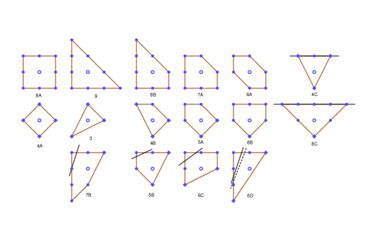
Figure 5.1. The polygon $P$ of all Gorenstein toric Fano surfaces.

Example 35.

In dimension 3, there are 18 isomorphism classes of smooth toric Fano 3-folds, see Table-1 in [NSY] (first version) for a list of them, and the labels used below. In [YZ], Yotsutani and Zhou found some criterions to determine the relative K-stability of toric varieties. They computed $\theta_{P}$ for these 3-folds, see Table 2 in [YZ]. Since $\ell_{P}=V_{P}^{-1}\left(1-\theta_{P}\right)$, by their computation results, we can determine the relative Ding stability of these 3-folds.

In 18 classes, $\{\mathbb{P}^{3},\mathcal{B}_{4},\mathcal{C}_{3},\mathcal{C}_{5},\mathcal{F}_{1}\}$ have vanishing Futaki invariant, hence they are uniformly relative D-stable and admit KE metrics; $\{\mathcal{B}_{2},\mathcal{B}_{3},\mathcal{C}_{1},\mathcal{C}_{4},\mathcal{E}_{3},\mathcal{E}_{4},\mathcal{F}_{2}\}$ are uniformly relative D-stable with nonvanishing Futaki invariant; the rests $\{\mathcal{B}_{1},\mathcal{C}_{2},\mathcal{D}_{1},\mathcal{D}_{2},\mathcal{E}_{1},\mathcal{E}_{2}\}$ are relatively D-unstable.

For the classification in dimension 4, see [NSY].

Remark 36.

In dimension $\leq 4$, there is no smooth toric Fano manifold that is non-uniformly relative D-stable. We do not know whether such manifolds exist in higher dimension. We also do not know whether there exists a rational polytope $P$ such that $P\cap\{\ell_{P}=0\}$ is a face of $P$ with codimension $>1$.

5.4. Existence results in the uniformly stable case

In the case of $\inf_{P}\ell>0$, the equation $\ell(d\phi)\textrm{MA}(\phi)=e^{-\phi}$ had been studied in [BB]. Theorem 1.1 in [BB] yields,

Theorem 37.

[BB] (1) Let $P$ be a convex body containing $0$ in its interior and suppose that $\inf_{P}\ell_{P}>0$. Then there exists a smooth and strictly convex function $\phi\in\textrm{PSH}_{b}(P)$ satisfying

$$\ell(d\phi)\textrm{MA}(\phi)=e^{-\phi},\ \textrm{on}\ \mathbb{R}^{n},$$

and $d\phi:\mathbb{R}^{n}\rightarrow\mathrm{Int}(P)$ is a diffeomorphism. Such $\phi$ is unique up to translations.

(2) Let $X_{P}$ be a toric Fano variety associated to polytope $P$ with $\inf_{P}\ell_{P}>0$. The above solution $\phi$ gives a $S_{N}$-invariant weak Mabuchi soliton on $X_{P}$, in the sense that its potential is continuous on $X_{P}$ and smooth on $T_{N}\subset X_{P}$.

When $X_{P}$ is smooth (i.e. $P$ is Delzant), we can obtain a smooth Mabuchi soliton via the continuation method in [WZ].

Theorem 38.

[WZ] Let $X$ be a toric Fano manifold associated to Delzant polytope $P$ with $\inf_{P}\ell_{P}>0$, then $X$ admits a smooth $S_{N}$-invariant Mabuchi soliton.

Proof.

The proof is almost a duplication of [WZ], so we just sketch it. Consider the following equations parameterized by $t\in[0,1]$ (compare with (2.2)),

$$\left(1-\theta_{Z}(\omega_{u_{t}})\right)\omega_{u_{t}}^{n}=e^{h_{r}-tu_{t}}\omega_{r}^{n},$$

where the reference metric $\omega_{r}$ is $S_{N}$-invariant. Let $\mathcal{I}\subset[0,1]$ be the set of $t$ such that the equation is solvable. Our aim is to show $1\in\mathcal{I}$. $0\in\mathcal{I}$ is shown in the Appendix of [LZ] and the openness of $\mathcal{I}$ follows from the implicit function theorem. All that remains is to show $\mathcal{I}$ is closed, it suffices to establish a uniform estimate for $u_{t}$. By the $S_{N}$-invariance, the above equation can be reduced to

$$\ell(d\phi_{t})\textrm{MA}(\phi_{t})=e^{-t\phi_{t}-(1-t)\phi_{r}},\ \textrm{on}\ \mathbb{R}^{n},$$

where $\phi_{t}$ and $\phi_{r}$ are the corresponding convex functions of $\omega_{u_{t}}$ and $\omega_{r}$, we have $u_{t}=\phi_{t}-\phi_{r}$. Since the term $\ell(d\phi_{t})$ is bounded above and below (away from zero), the next arguments in [LZ] also work in our setting, then we obtain a uniform estimate for $u_{t}$. ∎

Remark 39.

Above theorem is also covered by Theorem 1.5 in [LZ], where they considered the more general group compactifications. As in [SZ], the above theorem can be extended to toric Fano orbifolds, then it will include the uniformly relative D-stable Fano surfaces in Example 34.

6. Partial coercivity

In this section, when $\ell_{P}\geq 0$ on $P$, we establish a partial coercive inequality for $D_{\ell}$.

Theorem 40.

(Partial coercivity) Let $P\subset\mathbb{R}^{n}$ be a polytope containing $0$ in its interior. Suppose that $\ell_{P}\geq 0$ on $P$. Then for any $\epsilon\in(0,1)$ there is a constant $C_{\epsilon}>0$ depending on $P$ and $\epsilon$ such that

(6.1) $$D_{\ell}(\phi)\geq\epsilon\int_{P}\phi^{*}\ell-C_{\epsilon}$$

for all $\phi\in\mathcal{E}^{1}(P)$ such that $\phi\geq\phi(0)=0$. Then we have $D_{\ell}(\phi)\geq\epsilon J_{\ell}^{T}(\phi)-C_{\epsilon}$ for all $\phi\in\mathcal{E}^{1}(P)$. In particular, $D_{\ell}$ is bounded from below.

Its proof needs a subsolution of the equation for Mabuchi solitons.

Lemma 41.

(Existence of Subsolution) Let $P\subset\mathbb{R}^{n}$ be a polytope containing $0$ in its interior. Suppose that $\ell_{P}\geq 0$ on $P$. Then there is a smooth and strictly convex $\phi\in\textrm{PSH}_{b}(P)$ such that $C\cdot\ell_{P}(d\phi)\mathrm{MA}(\phi)\geq e^{-\phi}$ on $\mathbb{R}^{n}$ for some constant $C>0$.

Proof.

Let $\varphi(x)=\log\sum_{p}e^{\left\langle x,p\right\rangle}$, where the sum is over all vertices of $P$. It can be directly checked that $\varphi$ is smooth, strictly convex and $\psi_{P}\leq\varphi(x)\leq\psi_{P}+C_{P}$, on $\mathbb{R}^{n}$ for some constant $C_{P}$. We show that $\phi(x)\coloneqq R\varphi(\frac{x}{R})$ could satisfy the desired conditions when $R$ is sufficiently large.

Firstly, $\phi$ is still in $\textrm{PSH}_{b}(P)$ and we have

$$\ell(d\phi)(Rx)=\frac{\sum_{p}\ell(p)e^{\left\langle x,p\right\rangle}}{\sum_{p}e^{\left\langle x,p\right\rangle}},\ \mathrm{MA}(\phi)(Rx)=\frac{1}{R^{n}}\mathrm{MA}(\varphi)(x)$$

and $e^{-\phi(Rx)}=\left(\sum_{p}e^{\left\langle x,p\right\rangle}\right)^{-R}$. In order to make $C\cdot\ell(d\phi)\mathrm{MA}(\phi)\geq e^{-\phi}$ holds on $\mathbb{R}^{n}$, by taking the logarithm, it is sufficient to make

(6.2) $$\log\sum_{p}\ell(p)e^{\left\langle x,p\right\rangle}+\log\mathrm{MA}(\varphi)(x)+(R-1)\varphi(x)-n\log R$$

is bounded from below. If we can bound the first two terms from below by some $-C_{1}\psi_{P}-C_{2}$ (where $C_{i}>0$ only depends on $P$), then by $\varphi\geq\psi_{P}$, we can take $R$ to be sufficiently large so that the whole (6.2) is bounded from below.

(1) For the first term, we have

$$\sum_{p}\ell(p)e^{\left\langle x,p\right\rangle}=\sum_{\ell(p)>0}\ell(p)e^{\left\langle x,p\right\rangle}\geq\delta\sum_{\ell(p)>0}e^{\left\langle x,p\right\rangle},$$

where the second sum is over all vertices $p$ such that $\ell(p)>0$. Note that $\log\sum_{\ell(p)>0}e^{\left\langle x,p\right\rangle}\geq\psi_{Q}$, where $\psi_{Q}(x)=\sup_{y\in Q}\left\langle x,y\right\rangle$ and $Q$ is the convex hull of all vertices $p$ of $P$ such that $\ell(p)>0$. Taking a $K\gg 1$ such that $-Q\subset K\cdot P$, then $\psi_{Q}\geq-K\psi_{P}$. Finally, we have

$$\log\sum_{p}\ell(p)e^{\left\langle x,p\right\rangle}\geq-K\psi_{P}+\log\delta,\ \textrm{on}\ \mathbb{R}^{n}.$$

(2) For the second term: $\log\mathrm{MA}(\varphi)$, we compute

$$\varphi_{ij}(x)=\sum_{p}(p_{i}-\bar{p}_{i})(p_{j}-\bar{p}_{j})\frac{e^{\left\langle x,p\right\rangle}}{\sum_{p}e^{\left\langle x,p\right\rangle}},\ \bar{p}_{i}=\frac{\sum_{p}p_{i}e^{\left\langle x,p\right\rangle}}{\sum_{p}e^{\left\langle x,p\right\rangle}}.$$

Our aim is to bound $\log\det[\varphi_{ij}]$ from below by some $-C_{1}\psi_{P}-C_{2}$. First we can take the factor $\sum_{p}e^{\left\langle x,p\right\rangle}$ (in $\varphi_{ij}$) out of the determinant. Next we give a lower bound for the eigenvalues of matrix $H_{ij}(x)\coloneqq\sum_{p}(p_{i}-\bar{p}_{i})(p_{j}-\bar{p}_{j})e^{\left\langle x,p\right\rangle}$. For any $\xi\in\mathbb{R}^{n}$, we have

$$\sum_{i,j}H_{ij}\xi_{i}\xi_{j}=\sum_{p}\left\langle p-\bar{p},\xi\right\rangle^{2}e^{\left\langle x,p\right\rangle}\geq e^{\min_{p}\left\langle x,p\right\rangle}\sum_{p}\left\langle p-\bar{p},\xi\right\rangle^{2},$$

where $\bar{p}=(\bar{p}_{1},\cdots,\bar{p}_{n})$ depends on $x$. We claim there is a $\gamma>0$ depending on $P$ such that $\sum_{p}\left\langle p-\bar{p},\xi\right\rangle^{2}\geq\gamma\left|\xi\right|^{2}$ for all $x,\ \xi\in\mathbb{R}^{n}$. Consider a continuous function $Q(\eta,\xi)=\sum_{p}\left\langle p-\eta,\xi\right\rangle^{2}$ defined on compact space $Y\coloneqq P\times\mathbb{S}^{n-1}$. Then we must have $\inf_{Y}Q>0$, otherwise $Q=0$ at some point in $Y$, but this never happens unless $P$ is contained in a hyperplane. Note that $\bar{p}\in P$, then the claim follows from $\inf_{Y}Q>0$.

It follows that $\sum_{i,j}H_{ij}\xi_{i}\xi_{j}\geq e^{\min_{p}\left\langle x,p\right\rangle}\gamma\left|\xi\right|^{2}$ for all $\xi\in\mathbb{R}^{n}$. This gives a lower bound for eigenvalues, so $\det H\geq e^{n\min_{p}\left\langle x,p\right\rangle}\gamma^{n}$, namely

$$\log\det H(x)\geq n\min_{p}\left\langle x,p\right\rangle+n\log\gamma,\ \textrm{for all}\ x\in\mathbb{R}^{n}.$$

Finally, we take a $K>0$ such that $-P\subset K\cdot P$, then

$$\min_{p}\left\langle x,p\right\rangle=-\sup_{p}\left\langle x,-p\right\rangle=-\psi_{-P}(x)\geq-K\psi_{P}.$$

Now we bound $\log\det[\varphi_{ij}]$ from below by some $-C_{1}\psi_{P}-C_{2}$. ∎

Remark 42.

This lemma is expected to hold for general convex bodies, but we can not take $\varphi(x)=\log\int_{P}e^{\left\langle x,y\right\rangle}dy$ and go through the same proof, since it may not belong to $\textrm{PSH}_{b}(P)$, e.g. $P=[-1,1]$.

Once we have a subsolution, (6.1) follows from the same method in Theorem 2.16 [BB].

Proof.

(of Theorem 40)

Step 1. By the above lemma, there is a smooth and strictly convex $\phi_{0}\in\textrm{PSH}_{b}(P)$ such that $\int_{\mathbb{R}^{n}}e^{-\phi_{0}}=1$ and

$$C\ \ell_{P}(d\phi_{0})\mathrm{MA}(\phi_{0})\geq e^{-\phi_{0}},\ \textrm{on}\ \mathbb{R}^{n}.$$

Firstly we show there exists $C_{1}>0$ depending on $\phi_{0}$ such that

(6.3) $$-\log\int e^{-\phi}dx\geq CE_{\ell}(\phi)-C_{1},$$

for all $\phi\in\mathcal{E}^{1}(P)$ with $\phi(0)=0$.

Since $\phi_{0}\in\textrm{PSH}_{b}(P)$, suppose $\psi_{P}\leq\phi_{0}+A$ for a constant $A$. By (3.2), $\phi(0)=0$ implies $\phi\leq\psi_{P}$, hence $\phi-A\leq\phi_{0}$. Let $\{\phi_{t}\}_{0\leq t\leq 1}$ be the toric geodesic segment connecting $\phi_{0}$ with $\phi_{1}\coloneqq\phi-A$. Since $\phi_{0}\geq\phi_{1}$, we have $\frac{\partial\phi_{t}}{\partial t}|_{t=0}\leq 0$. Then by the convexity of $D_{\ell}$ and $D_{\ell}(\phi_{1})=D_{\ell}(\phi)$, we have

$$D_{\ell}(\phi)-D_{\ell}(\phi_{0}) \geq \frac{d}{dt}D_{\ell}(\phi)|_{t=0}=\int_{\mathbb{R}^{n}}\frac{\partial\phi_{t}}{\partial t}|_{t=0}\left(e^{-\phi_{0}}-\ell(d\phi_{0})\mathrm{MA}(\phi_{0})\right)$$

$$\geq (C-1)\int_{\mathbb{R}^{n}}\frac{\partial\phi_{t}}{\partial t}|_{t=0}\ell(d\phi_{0})\mathrm{MA}(\phi_{0})$$

$$= (C-1)\left(E_{\ell}(\phi-A)-E_{\ell}(\phi_{0})\right).$$

The last equality since $E_{\ell}$ is affine along $\{\phi_{t}\}$. Since $D_{\ell}(\phi)=-\log\int e^{-\phi}-E_{\ell}(\phi)$, (6.3) follows.

Step 2. For any normalized $\phi\in\mathcal{E}^{1}(P)$ and $0<r<1$, we put $\phi^{(r)}\coloneqq r\phi(\frac{x}{r})$ into (6.3), since $E_{\ell}(\phi^{(r)})=-\int_{P}\phi^{(r)*}\ell=rE_{\ell}(\phi)$, it yields

$$-\log\int e^{-r\phi}dx\geq rCE_{\ell}(\phi)-C_{1}+n\log r.$$

Since $\phi\geq 0$, we have

$$D_{\ell}(\phi)\geq-\log\int e^{-r\phi}dx-E_{\ell}(\phi)=(1-rC)\int_{P}\phi^{*}\ell-C(r).$$

Finally, when we take $r$ to be sufficiently small, then (6.1) follows.

For any $\phi\in\mathcal{E}^{1}(P)$, take $a\in\mathbb{R}^{n}$ such that $\tilde{\phi}(x)=\phi(x+a)-\phi(a)$ is normalized at $0$. Then we put $\tilde{\phi}$ into (6.1), and note that $D_{\ell}(\tilde{\phi})=D_{\ell}(\phi)$ and

$$J_{\ell}^{T}(\phi)=J_{\ell}^{T}(\tilde{\phi})=\int_{P}(\tilde{\phi})^{*}\ell,$$

by (5.3), the desired inequality follows. ∎

7. The non-uniformly stable case

In this section, we deal with the borderline case: $\inf_{P}\ell_{P}=0$. In Example 34, polygon 4C and 8C are such cases. There does not exist smooth solutions in this case, since the equation (2.2) implies $1-\theta_{Z}(\omega)>0$ on $X$, so $\inf_{P}\ell>0$. However, as the below example shows, there may exist some weak solutions with mild singularities.

Example 43.

(Mabuchi soliton with conic singularities) The polygon 8C in Example 34 is given by

$$P=\{(y_{1},y_{2})\mid-y_{2}\geq-1,y_{1}+y_{2}\geq-1,-y_{1}+y_{2}\geq-1\}$$

with vertices $(0,-1)$, $(2,1)$, $(-2,1)$. The associated toric Fano surface $X_{P}$ is $\mathbb{P}(1,1,2)$, a weighted projective plane. It has only one singular point $[0,0,1]$, which is corresponding to the vertex $(0,-1)$. The Ricci affine function is $\ell_{P}=\frac{3}{8}-\frac{3}{8}y_{2}$.

We construct an explicit solution for Mabuchi solitons. Let

$$\phi_{FS}(x)\coloneqq\log\sum_{\textrm{vertex}\ p}e^{\left\langle x,p\right\rangle}=\log\left(e^{-x_{2}}+e^{2x_{1}+x_{2}}+e^{-2x_{1}+x_{2}}\right)$$

and $\phi(x)\coloneqq 4\phi_{FS}(\frac{x}{4})$. We see $\phi\in\textrm{PSH}_{b}(P)$ is smooth and strictly convex on $\mathbb{R}^{2}$. By Wolfram Mathematica, we find

(7.1) $$\ell(d\phi)\mathrm{MA}(\phi)=3e^{-\phi}.$$

Thus it gives a Mabuchi soliton at least on the dense torus $T_{N}$. To investigate its behavior near the boundary divisors, we need to know its Legendre dual. It is not easy to compute it directly, instead, we define

$$v(y) = \mathbf{2}(1-y_{2})\log(1-y_{2})+(1+y_{1}+y_{2})\log(1+y_{1}+y_{2})$$

$$+(1-y_{1}+y_{2})\log(1-y_{1}+y_{2})$$

and $\psi=v^{*}$. Since $v$ is bounded on $P$, so $\psi\in\textrm{PSH}_{b}(P)$. A direct computation (on $v$) shows that $\ell(d\psi)\mathrm{MA}(\psi)=\frac{3}{64}e^{-\psi}$. By the uniqueness of the solution for (7.1), there is $a\in\mathbb{R}^{n}$ and $c\in\mathbb{R}$ such that $\psi(x)=\phi(x+a)+c$, thus $\phi^{*}$ equals to $v$ up to an affine function (given by $a$ and $c$).

Note (43) is exactly the Guillemin’s model symplectic potential except the coefficient 2. Let $\triangle\subset X$ be the prime divisor corresponding to the facet $\{\ell=0\}=\{y_{2}=1\}$. Note $\triangle$ does not contain the singular point. By Proposition 3.1 [SW], we know $\phi$ has conic singularities along $\triangle$ with angle $\pi$. Consider the equation on $X_{P}$,

$$\left(1-\theta_{Z}(\omega_{u})\right)\omega_{u}^{n}=e^{-u+h_{r}}\omega_{r}^{n},$$

where $\omega_{r}$ is a smooth reference metric and $\omega_{u}=i\partial\bar{\partial}\phi$, $\phi$ is the solution above. Comparing with smooth solutions, a main difference is that the term $\omega_{u}^{n}$ has a pole along $\triangle$ and $1-\theta_{Z}=\ell(d\phi)$ vanishes along $\triangle$, so they together make the RHS is bounded from above and below (away from zero). Taking $i\partial\bar{\partial}$ on both sides, $Ric(\omega_{u})$ contributes a current $\pi[\triangle]$, but $i\partial\bar{\partial}\log\left(1-\theta_{Z}(\omega_{u})\right)$ also contributes a current $\pi[\triangle]$ by the Poincaré-Lelong equation, so two currents are canceled by each other.

We can also write down an explicit solution for polygon 4C. For more examples, take $a\in\mathbb{N}$, then

$$P_{a}\coloneqq\{(y_{1},y_{2})\mid-y_{2}\geq-1,ay_{1}+y_{2}\geq-1,-ay_{1}+y_{2}\geq-1\}$$

is non-uniformly stable. Since $\ell=C_{a}(1-y_{2})$, where $C_{a}>0$ is a constant.

Next we establish a general existence result in the case of $\inf_{P}\ell_{P}=0$ ($\inf_{P}\ell_{P}>0$ is also included). The framework of our proof is same to [BB], via the variational method and relying on the partial coercivity (6.1), but we need some new techniques to remedy the absence of a positive lower bound for $\ell_{P}$.

Theorem 44.

Let $P\subset\mathbb{R}^{n}$ be a polytope containing $0$ in its interior. Suppose that $\ell_{P}\geq 0$ on $P$. Then there exists $\phi\in\textrm{PSH}_{b}(P)$ satisfying

$$\mathrm{MA}_{\ell}(\phi)=\frac{e^{-\phi}}{\int_{\mathbb{R}^{n}}e^{-\phi}},\ \textrm{on}\ \mathbb{R}^{n}$$

in the sense of Alexandrov. The Legendre dual $\phi^{*}$ is Hölder continuous on $P$ for any exponent $\gamma\in(0,1)$. In the case of $\dim P\cap\{\ell=0\}\leq\frac{n}{2}$ (including the case that the intersection is empty), we know $\phi$ is smooth and strictly convex on $\mathbb{R}^{n}$, and $d\phi$ gives a diffeomorphism from $\mathbb{R}^{n}$ to $\mathrm{Int}(P)$.

Proof.

(1) Since $D_{\ell}$ is bounded below and invariant under translations, there is a sequence of normalized functions $\{\phi_{j}\}\subset\mathcal{E}^{1}(P)$ such that $D_{\ell}(\phi_{j})\rightarrow\inf_{\mathcal{E}^{1}(P)}D_{\ell}$, where “normalized” means $\phi_{j}\geq\phi_{j}(0)=0$ or equivalently $\phi_{j}^{*}\geq\phi_{j}^{*}(0)=0$. The partial coercivity (6.1) implies $\int_{P}\phi_{j}^{*}\ell\leq C$. By a compactness result ([BB] Proposition 2.8), after passing to a subsequence, we assume $\phi_{j}$ converges to a $\phi\in\textrm{PSH}(P)$ uniformly over compact subsets in $\mathbb{R}^{n}$. Note $\phi$ is also normalized.

Since $\phi^{*}\leq\liminf_{j}\phi_{j}^{*}$, by Fatou’s lemma, we have

(7.3) $$\int_{P}\phi^{*}\ell\leq\int_{P}\liminf_{j}\phi_{j}^{*}\ell\leq\liminf_{j}\int_{P}\phi_{j}^{*}\ell\leq C.$$

This implies $\phi^{*}<\infty$ a.e. on $P$. Since $\phi^{*}$ is convex, it must have $\phi^{*}<\infty$ on $\mathrm{Int}(P)$, so $\phi\in\mathcal{E}(P)$. In particular, $\phi$ is proper on $\mathbb{R}^{n}$, thus $\int_{\mathbb{R}^{n}}e^{-\phi}<\infty$. Note that we can not assert $\phi\in\mathcal{E}^{1}(P)$ yet.

(2) We show $\lim_{j}\int e^{-\phi_{j}}=\int e^{-\phi}$. In [BB] (2.17), this follows from a Skoda type uniform estimate. Here we give another proof.

We claim that $\{\phi_{j}^{*}\}$ are uniformly bounded above on $\frac{1}{2}P$. As a finite-valued convex function on $\frac{1}{2}P$, $\phi_{j}^{*}$ can attain the maximum at some vertex of $\frac{1}{2}P$. At each vertex $v$ of $\frac{1}{2}P$, we take a ball $B_{r}(v)\subset\subset\frac{2}{3}P$. Suppose that $\ell\geq\delta>0$ on $\frac{2}{3}P$. By Jensen’s inequality,

$$\phi_{j}^{*}(v)\leq\frac{1}{\left|B_{r}\right|}\int_{B_{r}(v)}\phi_{j}^{*}\leq\frac{1}{\left|B_{r}\right|\delta}\int_{\frac{2}{3}P}\phi_{j}^{*}\ell\leq\frac{1}{\left|B_{r}\right|\delta}\int_{P}\phi_{j}^{*}\ell\leq\frac{C}{\left|B_{r}\right|\delta}.$$

Thus we have $\sup_{\frac{1}{2}P}\phi_{j}^{*}\leq C$, this is the claim. It follows that $\phi_{j}\geq\frac{1}{2}\psi_{P}-C$ on $\mathbb{R}^{n}$.

For any $\epsilon>0$, since $\int_{B_{R}^{c}}e^{-\phi_{j}}\leq e^{C}\int_{B_{R}^{c}}e^{-\frac{1}{2}\psi_{P}}$, there exists a $R(\epsilon)>0$ such that $\int_{B_{R}^{c}}e^{-\phi_{j}}<\epsilon$ for all $j\geq 1$ and $\int_{B_{R}^{c}}e^{-\phi}<\epsilon$. Since

$$\left|\int_{\mathbb{R}^{n}}e^{-\phi_{j}}-\int_{\mathbb{R}^{n}}e^{-\phi}\right|\leq\int_{B_{R}}\left|e^{-\phi_{j}}-e^{-\phi}\right|+\int_{B_{R}^{c}}e^{-\phi_{j}}+\int_{B_{R}^{c}}e^{-\phi}$$

and $\phi_{j}$ uniformly converges to $\phi$ on $B_{R}$, we obtain $\lim_{j}\int e^{-\phi_{j}}=\int e^{-\phi}$.

The Skoda type estimate in [BB] (2.17) can be also obtained by the above method.

(3) Combing (7.3) with (2), we have

(7.4) $$D_{\ell}(\phi)\leq\liminf_{j}D_{\ell}(\phi_{j})=\inf_{\mathcal{E}^{1}(P)}D_{\ell}$$

Consider a perturbation $\phi+t\eta$, where $\eta$ is a compact supported smooth function on $\mathbb{R}^{n}$. Since it may be not convex, we take the envelop

$$\phi_{t}(x)\coloneqq\sup\{\psi(x)\mid\textrm{PSH}(P)\ni\psi\leq\phi+t\eta\}=(\phi+t\eta)^{**},$$

where $**$ is taking the Legendre dual twice, see [BB] section 2.6. Since $\eta$ is bounded, we see $\left|\phi_{t}-\phi\right|$ is also bounded on $\mathbb{R}^{n}$. Since $\phi\in\mathcal{E}(P)$ and $\int_{P}\phi^{*}\ell<\infty$, thus $\phi_{t}\in\mathcal{E}(P)$ and $\int_{P}\phi_{t}^{*}\ell<\infty$.

Although we do not know $\phi_{t}\in\mathcal{E}^{1}(P)$, but we still have $\inf_{\mathcal{E}^{1}(P)}D_{\ell}\leq D_{\ell}(\phi_{t})$. Indeed, by the regularization Lemma 2.2 [BB], there exists a sequence $\varphi_{t}^{k}\in\textrm{PSH}_{b}(P)$ decreasing to $\phi_{t}$. Then by Fatou’s lemma, we have $\lim_{k}D_{\ell}(\varphi_{t}^{k})=D_{\ell}(\phi_{t})$. Since $D_{\ell}(\varphi_{t}^{k})\geq\inf_{\mathcal{E}^{1}(P)}D_{\ell}$, the inequality follows.

By (7.4), we have

$$D_{\ell}(\phi)\leq D_{\ell}(\phi_{t})\leq-\log\int e^{-(\phi+t\eta)}-E_{\ell}(\phi_{t})\eqqcolon h(t).$$

Note that $h(0)=D_{\ell}(\phi)$, so $h(t)$ attains a minimum at $t=0$. By a slight modification of Proposition 2.13 [BB] (replacing $dy$ by $\ell dy$ in its proof), it follows that $E_{\ell}(\phi_{t})=-\int_{P}(\phi+t\eta)^{*}\ell$ is differentiable at $t=0$ with derivative $\int_{\mathbb{R}^{n}}\eta\mathrm{MA}_{\ell}(\phi)$. Hence $h^{\prime}(0)=0$ for all $\eta$, it implies that $\phi$ satisfies

$$\mathrm{MA}_{\ell}(\phi)=\frac{e^{-\phi}}{\int e^{-\phi}}$$

in the sense of Alexandrov. By adding a constant, we assume $\int e^{-\phi}=1$. It means that for any Borel subset $E\subset\mathbb{R}^{n}$, we have

(7.5) $$\int_{\partial\phi(E)}\ell=\int_{E}e^{-\phi}.$$

(4) We show $\phi\in\textrm{PSH}_{b}(P)$. To simplify the notations, we denote $u=\phi^{*}$. By (7.3), we know $\int_{P}u\ell<\infty$. Moreover, for any $q\geq 1$ we have

(7.6) $$\int_{P}\left|du\right|^{q}\ell=\int_{\mathbb{R}^{n}}\left|x\right|^{q}\mathrm{MA}_{\ell}(\phi)=\int_{\mathbb{R}^{n}}\left|x\right|^{q}e^{-\phi}<\infty.$$

The last finiteness since $\phi\in\mathcal{E}(P)$ and (3.4). Note the LHS integral is well-defined, since $u$ is convex hence differentiable a.e.

We state a weighted Poincaré inequality due to Chua and Wheeden [CW] Theorem 1.1, which says for a bounded convex domain $\Omega\subset\mathbb{R}^{n}$ with a weight function $w=\rho^{k}$ (where $k\geq 0$, $\rho\geq 0$ is concave on $\Omega$) and any $1\leq q\leq p<\infty$, there exists a constant $B_{p,q}$ such that

$$\left(\int_{\Omega}\left|f-\frac{\int_{\Omega}fw}{\int_{\Omega}w}\right|^{q}wdx\right)^{1/q}\leq B_{p,q}\cdot\left(\int_{\Omega}w\right)^{\frac{1}{q}-\frac{1}{p}}\mathrm{diam}(\Omega)\left(\int_{\Omega}\left|df\right|^{p}wdx\right)^{1/p}$$

for any Lipschitz function $f$ on $\Omega$. Where $B_{p,q}$ only depends on $p,q$.

For any $\delta\in(0,1)$, $u=\phi^{*}$ is Lipschitz over $\delta\cdot P\subset P$. We apply the above inequality to datum $(\Omega,\rho,k,p,q,f)=(\delta P,\ell,1,q,q,u)$, then there is a constant $C_{q}$ (only depending on $q$) such that

$$\int_{\delta P}\left|u-\frac{\int_{\delta P}u\ell}{\int_{\delta P}\ell}\right|^{q}\ell\leq C_{q}\cdot\mathrm{diam}(\delta P)^{q}\int_{\delta P}\left|du\right|^{q}\ell$$

holds for any $\delta\in(0,1)$. By (7.6), the RHS is uniformly bounded, let $\delta\rightarrow 1$ we know $\int_{P}u^{q}\ell<\infty$ for any $q\geq 1$.

Now we can get rid of $\ell.$ For any $r\geq 1$, by the Hölder inequality,

$$\int_{P}u^{r}=\int_{P}u^{r}\ell^{\frac{1}{p}}\ell^{-\frac{1}{p}}\leq\left(\int_{P}u^{pr}\ell\right)^{\frac{1}{p}}\left(\int_{P}\ell^{-\frac{p^{\prime}}{p}}\right)^{\frac{1}{p^{\prime}}},$$

where $p,p^{\prime}>1$ are conjugate to each other. We take $\frac{p^{\prime}}{p}=p^{\prime}-1$ is sufficiently small such that $\int_{P}\ell^{-p^{\prime}/p}<\infty$. Then it follows that $\int_{P}u^{r}<\infty$ for all $r\geq 1$, in particular $\phi\in\mathcal{E}^{1}(P)$. Applying Hölder’s inequality again to (7.6), we can show $\int_{P}\left|du\right|^{r}<\infty$ for all $r\geq 1$. By the Sobolev imbedding theorem for domains with Lipschitz boundary, we conclude that $u=\phi^{*}$ is Hölder continuous over $P$ for any exponent $\gamma\in(0,1)$. In particular, $\phi^{*}$ is bounded on $P$, so $\phi\in\textrm{PSH}_{b}(P)$.

(5) Smoothness of $\phi$. When $\inf_{P}\ell>0$, since $\phi$ satisfies $\mathrm{MA}(\phi)=\frac{e^{-\phi}}{\ell(\partial\phi)}$ (in the sense of Alexandrov) and the RHS is locally bounded above and from below away from $0$, the smoothness of $\phi$ directly follows from the regularity results of Caffarelli, as in [BB] section 2.12. When $\inf_{P}\ell=0$, we can not obtain a local upper bound for $\mathrm{MA}(\phi)$ directly. But we can do this under the assumption: $\dim P\cap\{\ell=0\}\leq\frac{n}{2}$ (including $\inf_{P}\ell>0$), then we can show $\phi$ is smooth.

Let $K\subset\mathbb{R}^{n}$ be a compact set, then $\partial\phi(K)\subset P$ is also compact. We will show that $\partial\phi(K)\cap\{\ell=0\}$ must be empty if $\dim P\cap\{\ell=0\}\leq\frac{n}{2}$. If this is not true, there is $p\in\partial\phi(x_{0}),x_{0}\in K$ such that $\ell(p)=0$. Let

$$S(p)\coloneqq\{\xi\in N_{\mathbb{R}}\mid\left\langle\xi,p\right\rangle\geq\left\langle\xi,y\right\rangle\ \textrm{for all}\ y\in P\},$$

which is a cone of dimension $\geq n-\dim P\cap\{\ell=0\}$. We claim $\phi$ is affine over the set $x_{0}+S(p)$.

In fact, for any nonzero $\xi\in S(p)$, consider function $f(t)\coloneqq\phi(x_{0}+t\xi)$, which is convex in $t\in\mathbb{R}$. By the definition of sub-differentials, it is easy to see $\left\langle\xi,p\right\rangle\in\partial f(0)$. Suppose $f$ is differentiable at $t_{0}>0$ (almost everywhere), then for any $q\in\partial\phi(x_{0}+t_{0}\xi)\subset P$, we have $f^{\prime}(t_{0})=\left\langle\xi,q\right\rangle\leq\left\langle\xi,p\right\rangle$. The monotonicity of slopes of $f$ implies $f$ must be affine on $[0,\infty)$, i.e. $\phi(x_{0}+t\xi)=\phi(x_{0})+t\left\langle\xi,p\right\rangle$ for all $t\geq 0$. The claim follows, more specifically we have

(7.7) $$\phi(x_{0}+\xi)=\phi(x_{0})+\left\langle\xi,p\right\rangle,\ \textrm{for all}\ \xi\in S(p).$$

Next we show $\mathrm{MA}(\phi)$ is locally bounded from below. Let $F\subset\mathbb{R}^{n}$ be any bounded subset, suppose $\phi\leq C$ on $F$ and $\ell\leq C^{\prime}$ on $P$, then for any Borel subset $E\subset F$, by (7.5), we have

$$C^{\prime}\mathrm{MA}(\phi)(E)\geq\int_{\partial\phi(E)}\ell=\int_{E}e^{-\phi}\geq e^{-C}\left|E\right|,$$

thus $\mathrm{MA}(\phi)\geq\frac{1}{C^{\prime}}e^{-C}\ dx$ on $F$.

Now we use the assumption: $\dim P\cap\{\ell=0\}\leq\frac{n}{2}$, it implies $\dim S(p)\geq\frac{n}{2}$. Let

$$\psi(x)\coloneqq\phi(x)-\phi(x_{0})-\left\langle x-x_{0},p\right\rangle,$$

then $\psi\geq 0$ since $p\in\partial\phi(x_{0})$ and $\psi$ vanishes on $x_{0}+S(p)$ since (7.7). Taking a small ball $B$ intersecting $x_{0}+S(p)$, then $\mathrm{MA}(\psi)\geq\lambda\ dx$ on $B$ for some $\lambda>0$. But Lemma 2.3 in [Mo] says, if $\mathrm{MA}(\psi)\geq\lambda\ dx$ on a ball, $\psi$ can not vanish along a subspace of dimension $\geq\frac{n}{2}$. We obtain a contradiction, thus $\partial\phi(K)\cap\{\ell=0\}$ must be empty for any compact $K\subset\mathbb{R}^{n}$.

Now we can locally bound $\mathrm{MA}(\phi)$ from both sides. For any $R\gg 1$, take $K=\Omega_{R}\coloneqq\{\phi\leq R\}$, which is a compact convex set. Since we already show $\partial\phi(K)$ does not intersect $\{\ell=0\}$, so $\inf_{\partial\phi(K)}\ell>0$. For any Borel set $E\subset\Omega_{R}$, we have

$$\inf_{\partial\phi(K)}\ell\cdot\mathrm{MA}(\phi)(E)\leq\int_{\partial\phi(E)}\ell=\int_{E}e^{-\phi}\leq e^{-\min\phi}\left|E\right|.$$

Hence we have $\lambda dx\leq\mathrm{MA}(\phi)\leq\Lambda dx$ on $\Omega_{R}$ for some $\lambda,\ \Lambda>0$. By Corollary 4.11 [Fi], we know $\phi$ is strictly convex on $\Omega_{R}$, thus on whole $\mathbb{R}^{n}$. Note that strict convexity implies $\partial\phi(K)\cap\partial P=\emptyset$ for all compact $K\subset\mathbb{R}^{n}$. If this is not true, $\phi$ would be affine over a cone as the above $x_{0}+S(p)$.

With the strict convexity and the bounds for $\mathrm{MA}(\phi)$ from both sides, by Caffarelli’s interior $C^{1,\alpha}$ estimates (see Corollary 4.21 [Fi]), we know $\phi\in C_{\mathrm{loc}}^{1,\alpha}(\Omega_{R})$ for some $\alpha\in(0,1)$ depending on $R$. Thus the RHS of $\mathrm{MA}(\phi)=\frac{e^{-\phi}}{\ell(\partial\phi)}$ belongs to $C^{0,\alpha}$ locally, then by Caffarelli’s interior $C^{2,\alpha}$ estimates (see Corollary 4.43 [Fi]), we have $\phi\in C_{\mathrm{loc}}^{2,\alpha}(\Omega_{R})$. Finally, the smoothness of $\phi$ follows from a standard bootstrapping argument. ∎

Remark 45.

The solution $\phi$ obtained above is expected to be also smooth when $\dim P\cap\{\ell=0\}>\frac{n}{2}$. On the other hand, we make a conjecture about the asymptotics of $\phi^{*}$ near the boundary set $P\cap\{\ell=0\}$.

Assume $P$ is a Delzant polytope. For a vertex on $\{\ell=0\}$, by changing the coordinate, $P$ is locally given by

$$\{y\mid y_{i}\geq-1,\ 1\leq i\leq n\},\ \textrm{and}\ \ell(y)=\sum_{\alpha=1}^{p}c_{\alpha}(y_{\alpha}+1),\ c_{\alpha}>0.$$

Consider a model potential $u(y)=\sum_{i=1}^{n}(y_{i}+1)\log(y_{i}+1)+\lambda\cdot\ell\log\ell$. By a computation, in order to make the two sides of

$$\ell\cdot\det[u_{ij}]^{-1}=e^{u-y\cdot du}$$

have matching vanish factors along $P\cap\{\ell=0\}$, $\lambda$ must be equal to $\ell(0)^{-1}$. Hence we conjecture $\phi^{*}$ satisfies a modified Guillemin condition, namely

$$\phi^{*}=\frac{1}{\ell(0)}\ell\cdot\log\ell+\sum_{\alpha\in\Lambda}l_{\alpha}\log l_{\alpha}+w,$$

recall $l_{\alpha}(y)=\left\langle q_{\alpha},y\right\rangle+1$ are the defining functions of the facets of $P$, where $w(y)$ can be extended to a smooth function on a neighborhood of $P$. Note this form explains the coefficient 2 (so the cone angle $\pi$) in (43).

8. The unstable case and moment-weight equalities

8.1. Toric moment-weight inequalities

In this section, we derive a toric version of (1.7) from Jensen’s inequality.

Definition 46.

Let $P\subset\mathbb{R}^{n}$ be a convex body containing $0$ in its interior. We define

$$\mathfrak{B}_{P}=\left\{0\leq b(y)\in L^{2}(P)\mid\int_{P}bdy=1;\ \int_{P}y_{i}\ bdy=0,\ \textrm{for}\ 1\leq i\leq n\right\}.$$

We call $b(y)$ is a balancing density on $P$, since the barycenter of $(P,bdy)$ is the origin.

Proposition 47.

Let $X$ be a smooth toric Fano variety associated to Delzant polytope $P$. Then for any $\phi\in\mathcal{H}(-K_{X})^{S}$, we have $V_{P}^{-1}e^{h(\phi)}(d\phi^{*})\in\mathfrak{B}_{P}$.

Proof.

Recall $h(\phi)$ is the Ricci potential given by (3.10). Here we take $h(\phi)$ as a function defined on $N_{\mathbb{R}}$, so $e^{h(\phi)}(d\phi^{*})$ is a function on $P$. By (3.10), we see $\int_{P}e^{h(\phi)}(d\phi^{*})dy=V_{P}$. For $1\leq i\leq n$, we have ($C$ is a constant)

$$\int_{P}y_{i}e^{h(\phi)}(d\phi^{*})dy=C\int_{\mathbb{R}^{n}}\partial_{i}\phi\ e^{-\phi}dx=-C\int_{\mathbb{R}^{n}}\partial_{i}(e^{-\phi})dx.$$

Since $\phi(x)\geq\delta\left|x\right|-C^{\prime}$ for some $\delta$, $C^{\prime}>0$, applying the divergence formula on the ball $B_{R}$ and then let $R\rightarrow\infty$, we see the last integral is equal to zero. ∎

In the below, we use the $L^{2}$-norm $\left\|f\right\|_{2}^{2}\coloneqq\int_{P}\left|f\right|^{2}dy$ and its variant $\left\|f\right\|_{2,d\bar{y}}^{2}\coloneqq\frac{1}{V_{P}}\int_{P}\left|f\right|^{2}dy$. For simplicity, we will write $e^{h(\phi)}(d\phi^{*})$ as $e^{h(\phi)}$, which is a function on $P$.

Proposition 48.

(Toric Moment-Weight inequality) Let $X$ be a smooth toric Fano variety associated to Delzant polytope $P$.

(1) Let $\bar{f}=\frac{1}{V_{P}}\int_{P}fdy$, then we have

(8.1) $$\inf_{\phi\in\mathcal{H}(P)}\left\|e^{h(\phi)}-1\right\|_{2,d\bar{y}}\geq\sup_{\textrm{convex}\ f}\frac{-D^{\mathrm{NA}}(f)}{\left\|f-\bar{f}\right\|_{2,d\bar{y}}},$$

where the supremum is taking over all non-constant convex functions on $P$.

(2) Let $\pi:L^{2}(P,dy)\rightarrow\left\{l|_{P}\mid l\ \textrm{is affine}\right\}$ be the $L^{2}$-orthogonal projection, then we have

(8.2) $$\inf_{\phi\in\mathcal{H}(P)}\left\|e^{h(\phi)}-V_{P}\ell\right\|_{2,d\bar{y}}\geq\sup_{\textrm{convex}\ f}\frac{-D_{\ell}^{\mathrm{NA}}(f)}{\left\|f-\pi(f)\right\|_{2,d\bar{y}}},$$

where the supremum is taking over all non-affine convex functions on $P$.

Proof.

Let $g(y)$ be a continuous function on $P$ with $\int_{P}g=1$, we will take $g=V_{P}^{-1}$ and $\ell_{P}$. For any $\phi\in\mathcal{H}(P)$ and convex function $f$ on $P$, we have

$$\int_{P}f\left(V_{P}^{-1}e^{h(\phi)}-g\right)dy=-f(0)+\frac{1}{V_{P}}\int_{P}fe^{h(\phi)}dy-D_{g}^{\textrm{NA}}(f)\geq-D_{g}^{\textrm{NA}}(f).$$

The last step follows from Jensen’s inequality with Proposition 47.

Now take $g=V_{P}^{-1}$, note that $\int_{P}f\left(e^{h(\phi)}-1\right)dy=\int_{P}\left(f-\bar{f}\right)\left(e^{h(\phi)}-1\right)dy$. By the Cauchy-Schwarz inequality, we have

$$\int_{P}\left(f-\bar{f}\right)\left(e^{h(\phi)}-1\right)\frac{dy}{V_{P}}\leq\left(\int_{P}\left|f-\bar{f}\right|^{2}\frac{dy}{V_{P}}\right)^{1/2}\cdot\left(\int_{P}\left|e^{h(\phi)}-1\right|^{2}\frac{dy}{V_{P}}\right)^{1/2}.$$

Then (8.1) follows from the above two inequalities.

Take $g=\ell_{P}$, by Proposition 47, we have $\int_{P}\pi(f)\left(e^{h(\phi)}-V_{P}\ell\right)dy=0$. Then (8.2) follows in the same way. ∎

8.2. The maximal destabilizers

Let $P$ be a convex body containing $0$ in its interior. We define

$$\mathcal{C}_{2}(P)\coloneqq\{f:P\rightarrow\mathbb{R}\cup\{\infty\}\ \textrm{is convex}\mid f\in L^{2}(P)\}.$$

Note that for any $f\in\mathcal{C}_{2}(P)$, since it is convex and $f<\infty$ almost everywhere, it must have $f<\infty$ on $\textrm{Int}(P)$.

Let us consider the optimization problem on the RHS of (8.1), we need to minimize the functional

(8.3) $$W(f)\coloneqq\frac{D^{\textrm{NA}}(f)}{\left\|f-\bar{f}\right\|_{2}},\ \ f\in\mathcal{C}_{2}(P).$$

When the denominator is zero, we set $W=0$. If there is a minimizer, then we take it as the maximal destabilizer for Ding stability. In [Sz3], Székelyhidi had considered a similar problem for K-stability. As in [Sz3], we first try to minimize

$$W_{\ell}(f)\coloneqq\frac{D_{\ell}^{\textrm{NA}}(f)}{\left\|f-\pi(f)\right\|_{2}},\ f\in\mathcal{C}_{2}(P).$$

The advantage is that $W_{\ell}$ is invariant under addition by affine functions.

Lemma 49.

Let $P\subset\mathbb{R}^{n}$ be a convex body containing $0$ in its interior. Suppose that $\inf_{P}\ell_{P}<0$. Then there is a unique minimizer for $W_{\ell}$, denoted by $\hat{f}\in\mathcal{C}_{2}(P)$ such that

(8.4) $$\pi(\hat{f})=0\ \textrm{and}\ \int_{P}\hat{f}^{2}=\hat{f}(0).$$

The above two conditions are equivalent to require $\int_{P}\hat{f}l=0$ for all affine $l$ and $D_{\ell}^{\mathrm{NA}}(\hat{f})=-\left\|\hat{f}\right\|_{2}^{2}$.

Proof.

Since $W_{\ell}$ is invariant under addition of affine functions, we only need to minimize it over the normalized functions in $\mathcal{C}_{2}(P)$, i.e. satisfying $f\geq f(0)=0$.

Step 1: show $W_{\ell}$ is bounded below. By Lemma 7 [Sz3], there exists $C_{P}>0$ only depending on $P$ such that $\left\|f\right\|_{2}\leq C_{P}\left\|f-\pi(f)\right\|_{2}$ for all normalized $f\in\mathcal{C}_{2}(P)$. It follows that

$$D_{\ell}^{\textrm{NA}}(f)=\int_{P}f\ell\geq-\left\|l\right\|_{2}\left\|f\right\|_{2}\geq-C_{P}\left\|l\right\|_{2}\left\|f-\pi(f)\right\|_{2},$$

thus $W_{\ell}\geq-C_{P}\left\|l\right\|_{2}$.

Step 2: Let $\{f_{k}\}\subset\mathcal{C}_{2}(P)$ be a sequence of normalized convex functions such that $W_{\ell}(f_{k})\rightarrow\inf_{\mathcal{C}_{2}(P)}W_{\ell}<0$. Rescaling them such that $\int_{P}f_{k}^{2}=1$, by Hölder’s inequality, $\int_{P}f_{k}$ are bounded above. By Corollary 5.2.5 [D2], there is a subsequence (still denoted by $f_{k}$) converges to a function $\hat{f}:P\rightarrow\mathbb{R}\cup\{\infty\}$ uniformly over compact subsets of $\mathrm{Int}(P)$. Clearly, $\hat{f}$ is also a normalized convex function. By Fatou’s lemma, we have $\int_{P}\hat{f}^{2}\leq 1$ thus $\hat{f}\in\mathcal{C}_{2}(P)$.

Step 3: show $\hat{f}$ is a minimizer. By the weak compactness in $L^{2}(P)$, after passing to a subsequence, we can assume $f_{k}$ weakly converges in $L^{2}(P)$. The weak limit must be $\hat{f}$. It implies

$$D_{\ell}^{\textrm{NA}}(f_{k})=\int_{P}f_{k}\ell\rightarrow\int_{P}\hat{f}\ell=D_{\ell}^{\textrm{NA}}(\hat{f}),$$

thus

(8.5) $$\left\|f_{k}-\pi(f_{k})\right\|_{2}=\frac{D_{\ell}^{\textrm{NA}}(f_{k})}{W_{\ell}(f_{k})}\rightarrow\frac{D_{\ell}^{\textrm{NA}}(\hat{f})}{\inf W_{\ell}}.$$

The weak convergence also implies $\pi(f_{k})\rightarrow\pi(\hat{f})$ in the space of affine functions.

If $D_{\ell}^{\textrm{NA}}(\hat{f})=0$, (8.5) implies $\left\|f_{k}-\pi(f_{k})\right\|_{2}\rightarrow 0$, but this contradicts with $\int_{P}f_{k}^{2}=1$ and $\left\|f_{k}\right\|_{2}\leq C_{P}\left\|f_{k}-\pi(f_{k})\right\|_{2}$. Hence $D_{\ell}^{\textrm{NA}}(\hat{f})<0$ and so $\lim_{k}\left\|f_{k}-\pi(f_{k})\right\|_{2}>0$. By (8.5), we have

$$\frac{D_{\ell}^{\textrm{NA}}(\hat{f})}{\lim_{k}\left\|f_{k}-\pi(f_{k})\right\|_{2}}=\inf W_{\ell}.$$

Once we show

(8.6) $$\lim_{k}\left\|f_{k}-\pi(f_{k})\right\|_{2}\geq\left\|\hat{f}-\pi(\hat{f})\right\|_{2},$$

then it implies $W_{\ell}(\hat{f})\leq\inf W_{\ell}$, since $\hat{f}\in\mathcal{C}_{2}(P)$, thus $\hat{f}$ is a minimizer. In fact, for any compact subset $K\subset\textrm{Int}(P)$, since $f_{k}$ uniformly converges to $\hat{f}$ on $K$, we have

$$\left\|\hat{f}-\pi(\hat{f})\right\|_{2,K}=\lim_{k}\left\|f_{k}-\pi(f_{k})\right\|_{2,K}\leq\lim_{k}\left\|f_{k}-\pi(f_{k})\right\|_{2},$$

where $\left\|\cdot\right\|_{2,K}$ is the $L^{2}$-norm over $K$. Then we take $\sup_{K}$ of the LHS, (8.6) follows. Hence $\hat{f}$ is a minimizer.

Next we adjust $\hat{f}$ to satisfy (8.4). First we replace $\hat{f}$ by $\hat{f}-\pi(\hat{f})$, which is still a minimizer. After that, we have $\pi(\hat{f})=0$, equivalently $\int_{P}\hat{f}l=0$ for all affine $l$. Thus $\hat{f}(0)=-D_{\ell}^{\textrm{NA}}(\hat{f})>0$. Finally, we rescale $\hat{f}$ such that $\int_{P}\hat{f}^{2}=\hat{f}(0)$. Now we obtain a minimizer $\hat{f}$ satisfying (8.4). The statement for the equivalence of two normalization conditions is trivial.

Step 4: the uniqueness. Suppose $\hat{g}\in\mathcal{C}_{2}(P)$ is another minimizer satisfying (8.4), then $W_{\ell}(\hat{f})=W_{\ell}(\hat{g})$ and

$$W_{\ell}(\hat{g})=\frac{-\hat{g}(0)}{\left\|\hat{g}\right\|_{2}}=-\left\|\hat{g}\right\|_{2}.$$

It implies $\left\|\hat{f}\right\|_{2}=\left\|\hat{g}\right\|_{2}$ and $D_{\ell}^{\textrm{NA}}(\hat{f})=D_{\ell}^{\textrm{NA}}(\hat{g})<0$. Since $\hat{g}\neq\hat{f}$, $\hat{g}$ can not be proportional to $\hat{f}$, thus we have $\left\|\hat{f}+\hat{g}\right\|_{2}<2\left\|\hat{f}\right\|_{2}$. It follows that

$$W_{\ell}(\hat{f}+\hat{g})=\frac{2D_{\ell}^{\textrm{NA}}(\hat{f})}{\left\|\hat{f}+\hat{g}\right\|_{2}}<\frac{2D_{\ell}^{\textrm{NA}}(\hat{f})}{2\left\|\hat{f}\right\|_{2}}=W_{\ell}(\hat{f})=\inf_{\mathcal{C}_{2}(P)}W_{\ell}.$$

It is a contradiction, since $\hat{f}+\hat{g}\in\mathcal{C}_{2}(P)$. ∎

Next we study the structure of the minimizer $\hat{f}$ and give it more characterizations.

Theorem 50.

Let $P\subset\mathbb{R}^{n}$ be a convex body containing $0$ in its interior. Suppose that $\inf_{P}\ell_{P}<0$. Let $\hat{f}$ be the unique minimizer for $W_{\ell}$ satisfying (8.4), which is obtained in the above lemma. Then we have (1)-(4) below.

(1) Let $\mathfrak{b}\coloneqq\hat{f}+\ell_{P}$, then $\mathfrak{b}\geq 0$, and $\int_{P}\mathfrak{b}=1$, $\int_{P}y_{i}\mathfrak{b}=0$ for $1\leq i\leq n$, hence $\mathfrak{b}\in\mathfrak{B}_{P}$. Moreover, $\int_{P}\mathfrak{b}^{2}=\mathfrak{b}(0)$.

(2) $\mathfrak{b}$ is the unique element in $\mathfrak{B}_{P}$ with the minimum $L^{2}$-norm.

(3) For any convex $b\in\mathfrak{B}_{P}$, we have $\int_{P}b^{2}\geq b(0)$. The equality holds if and only if $b=\mathfrak{b}$.

(4) $\mathfrak{b}$ is a simple convex function, i.e. $\mathfrak{b}=\max\{0,\mathfrak{a}\}$, where $\mathfrak{a}$ is the unique affine function such that

(8.7) $$\int_{P\cap\{\mathfrak{a}>0\}}\mathfrak{a}=1,\int_{P\cap\{\mathfrak{a}>0\}}y_{i}\mathfrak{a}=0,\ \textrm{for}\ 1\leq i\leq n.$$

(5) If $\inf_{P}\ell_{P}\geq 0$, then $\ell_{P}$ is the unique element in $\mathfrak{B}_{P}$ with the minimum $L^{2}$-norm.

Proof.

(1) For any $h\in\mathcal{C}_{2}(P)$, we have $f_{t}\coloneqq\hat{f}+th\in\mathcal{C}_{2}(P)$ for $t\geq 0$. Since $\hat{f}$ is a minimizer for $W_{\ell}$, thus $\frac{d}{dt}W_{\ell}(f_{t})|_{t=0}\geq 0$. Combing with (8.4), it follows that

(8.8) $$-h(0)+\int_{P}h(\ell+\hat{f})\geq 0,\ \textrm{for all}\ h\in\mathcal{C}_{2}(P).$$

Let $\mathfrak{b}\coloneqq\ell+\hat{f}$, then (8.8) is equivalent to $D_{\mathfrak{b}}^{\textrm{NA}}(h)\geq 0$ for all $h\in\mathcal{C}_{2}(P)$. In particular, $D_{\mathfrak{b}}^{\textrm{NA}}(l)=0$ for all affine $l$. Then we have

$$D_{\mathfrak{b}}^{\textrm{NA}}(\mathfrak{b})=D_{\mathfrak{b}}^{\textrm{NA}}(\hat{f})=-\hat{f}(0)+\int_{P}\hat{f}\mathfrak{b}=-\hat{f}(0)+\int_{P}\hat{f}^{2}=0,$$

where we used (8.4). This is exactly $\int_{P}\mathfrak{b}^{2}=\mathfrak{b}(0)$. Finally, we show $\mathfrak{b}\geq 0$. If it is not true, let $\mathfrak{b}^{+}=\max\{\mathfrak{b},0\}\in\mathcal{C}_{2}(P)$, we have

$$D_{\mathfrak{b}}^{\textrm{NA}}(\mathfrak{b}^{+})=-\mathfrak{b}(0)+\int_{P}\mathfrak{b}\mathfrak{b}^{+}=-\int_{P}\mathfrak{b}^{2}+\int_{\{\mathfrak{b}\geq 0\}}\mathfrak{b}^{2}=-\int_{\{\mathfrak{b}<0\}}\mathfrak{b}^{2}<0,$$

note that $\mathfrak{b}$ is continuous on $\mathrm{Int}(P)$. This contradicts to (8.8), so we have $\mathfrak{b}\geq 0$.

(2) For any $b\in\mathfrak{B}_{P}$, by Jensen’s inequality with measure $bdy$, we have

$$\left\|\mathfrak{b}\right\|^{2}=\mathfrak{b}(0)\leq\int_{P}\mathfrak{b}\cdot bdy\leq\left\|\mathfrak{b}\right\|\cdot\left\|b\right\|,$$

thus $\left\|\mathfrak{b}\right\|\leq\left\|b\right\|$. Hence $\mathfrak{b}$ has the minimum $L^{2}$-norm. If $\left\|\mathfrak{b}\right\|=\left\|b\right\|$, then $b$ must be proportional to $\mathfrak{b}$. Since $\int_{P}b=\int_{P}\mathfrak{b}=1$, it forces $b=\mathfrak{b}$.

(3) For any convex $b\in\mathfrak{B}_{P}$, by Jensen’s inequality with measure $bdy$, we have $\int_{P}b^{2}=\int_{P}b\cdot bdy\geq b(0)$. If the equality holds, again by Jensen’s inequality,

$$\left\|b\right\|^{2}=b(0)\leq\int_{P}b\cdot\mathfrak{b}dy\leq\left\|b\right\|\cdot\left\|\mathfrak{b}\right\|,$$

thus $\left\|b\right\|\leq\left\|\mathfrak{b}\right\|$. Since $\mathfrak{b}$ has the minimum $L^{2}$-norm, (2) tells us $b=\mathfrak{b}$.

(4) Note that $\mathfrak{b}dy$ is a positive Radon measure with barycenter $0$. Since $\mathfrak{b}$ is convex, the condition $\int_{P}\mathfrak{b}\cdot\mathfrak{b}dy=\mathfrak{b}(0)$ means that Jensen’s inequality with measure $\mathfrak{b}dy$ takes equality. By the equality condition of Jensen’s inequality, $\mathfrak{b}$ must be affine over the convex hull of set $\{\mathfrak{b}>0\}$.

We claim that $\{\mathfrak{b}>0\}$ is convex. In fact, for any $y_{1},y_{2}\in\{\mathfrak{b}>0\}$, connecting them by a line segment $L$. Since $L$ is contained in the convex hull of $\{\mathfrak{b}>0\}$, so $\mathfrak{b}$ must be affine along $L$, this implies $L\subset\{\mathfrak{b}>0\}$, thus $\{\mathfrak{b}>0\}$ is convex. In particular, $\{\mathfrak{b}>0\}$ is connected. The only possibility is $\mathfrak{b}=\max\{0,\mathfrak{a}\}$ for some affine function $\mathfrak{a}$. Moreover, since $\mathfrak{b}\in\mathfrak{B}_{P}$, so $\mathfrak{a}$ should satisfy (8.7).

For the uniqueness of $\mathfrak{a}$, if there is an affine function $l$ satisfying (8.7) (replacing $\mathfrak{a}$ by $l$), then we have $\int_{P\cap\{l>0\}}l^{2}=l(0)$. Then $b\coloneqq\max\{0,l\}\in\mathfrak{B}_{P}$ and satisfies $\int_{P}b^{2}=b(0)$, by (3) we know $b=\mathfrak{b}$, so $l=\mathfrak{a}$.

(5) The proof is same to (2). ∎

The characteristic condition (8.7) for $\mathfrak{a}$ can be rephrased in a simple way, that is the Ricci affine function associated to $P\cap\{\mathfrak{a}\geq 0\}$ is $\mathfrak{a}$ itself. It gives a polynomial system with $n+1$ equations for the coefficients of $\mathfrak{a}$, the above theorem ensures that it admits a unique solution.

Definition 51.

Let $P\subset\mathbb{R}^{n}$ be a convex body containing $0$ in its interior, and $\ell_{P}$ is the associated Ricci affine function. We define the optimal balancing density of $P$ to be

$$\mathfrak{b}=\max\{0,\mathfrak{a}\},\ \textrm{when}\ \inf_{P}\ell_{P}<0;\ \ \mathfrak{b}=\ell_{P},\ \textrm{when}\ \inf_{P}\ell_{P}\geq 0.$$

Where $\mathfrak{a}$ is the unique affine function satisfying (8.7). By Theorem 50, in any case, $\mathfrak{b}$ is the unique element in $\mathfrak{B}_{P}$ with the minimum $L^{2}$-norm. We always have $\int_{P}\mathfrak{b}^{2}=\mathfrak{b}(0)$.

Corollary 52.

Let $P\subset\mathbb{R}^{n}$ be a convex body containing $0$ in its interior. Then we have

$$\inf\left\{W(f)\mid f\in\mathcal{C}_{2}(P)\right\}=-\left\|V_{P}^{-1}-\mathfrak{b}\right\|_{2},$$

and the infimum is attained by $\mathfrak{b}$. Recall $W(f)$ is defined by (8.3).

Proof.

For any $f\in\mathcal{C}_{2}(P)$, since $\mathfrak{b}\in\mathfrak{B}_{P}$, by Jensen’s inequality we have

$$D^{\textrm{NA}}(f)=D_{\mathfrak{b}}^{\textrm{NA}}(f)+\int_{P}f(V_{P}^{-1}-\mathfrak{b})dy\geq-\left\|f-\bar{f}\right\|_{2}\cdot\left\|V_{P}^{-1}-\mathfrak{b}\right\|_{2}.$$

Thus $W(f)\geq-\left\|V_{P}^{-1}-\mathfrak{b}\right\|_{2}$. On the other hand, taking $f=\mathfrak{b}$, since $\int_{P}\mathfrak{b}^{2}=\mathfrak{b}(0)$, we have $D^{\textrm{NA}}(\mathfrak{b})=-\left\|V_{P}^{-1}-\mathfrak{b}\right\|_{2}^{2}$. Thus $W(\mathfrak{b})=-\left\|V_{P}^{-1}-\mathfrak{b}\right\|_{2}$, all statements follow. ∎

Example 53.

For the unstable polygon 6D in Example 34,

$$P=\{(y_{1},y_{2})\mid y_{1}>-1,\ y_{2}<1,\ 3y_{1}-2y_{2}<1\}.$$

The associated toric Fano surface is $X_{P}=\mathbb{P}(1,2,3)$. By a computation, we have $\ell_{P}=\frac{2}{3}y_{1}-\frac{2}{9}y_{2}+\frac{5}{9}$. To determine the affine function $\mathfrak{a}$, firstly we need to know the rough location of $\{\mathfrak{a}=0\}$. For this, we use the following iteration scheme. Let $\ell_{0}\coloneqq\ell_{P}$, then for any $k\geq 1$, let $\ell_{k}$ be the Ricci affine function of the polytope $P\cap\{\ell_{k-1}\geq 0\}$. After several steps, when the set $\{\ell_{k}=0\}$ is approaching to be stable, we solve the polynomial system (8.7). By computer, we find

$$\mathfrak{a}=\frac{1}{162}\left(67+26\sqrt{7}\right)y_{1}-\frac{2}{243}\left(29+4\sqrt{7}\right)y_{2}+\frac{7}{486}\left(29+4\sqrt{7}\right).$$

In Figure 5.1, the set $\{\mathfrak{a}=0\}$ is showed by a dashed line. Note that the slope of this line is an irrational number, so $P\cap\{\mathfrak{a}\geq 0\}$ can not be the moment polytope of some toric variety.

Example 54.

Consider smooth toric Fano 3-fold $X=\mathbb{P}\left(\mathcal{O}_{\mathbb{P}^{2}}\oplus\mathcal{O}_{\mathbb{P}^{2}}(2)\right)$ (with label $\mathcal{B}_{1}$ in [NSY]), which is associated to polytope

$$P=\{y\in\mathbb{R}^{3}\mid y_{1}\geq-1,\ y_{2}\geq-1,\ y_{1}+y_{2}+2y_{3}\leq 1,\ -1\leq y_{3}\leq 1\}$$

with vertices $(0,-1,1),(-1,0,1),(-1,-1,1),(4,-1,-1),(-1,4,-1),(-1,-1,-1)$. It is also the blowup of $\mathbb{P}(1,1,1,2)$ at the unique singularity point $[0,0,0,1]$. By a computation, we have $V_{P}=\frac{31}{3}$ and $\ell_{P}=\frac{60}{349}y_{3}+\frac{57}{349}$. Thus $(-K_{X})^{3}=3!V_{P}=62$. We see $X$ is relatively D-unstable.

Next we determine the optimal balancing density. By the symmetry of $P$, we assume $\mathfrak{a}=a(y_{3}+b)$. The condition (8.7) requires $\int_{P\cap\{y_{3}>-b\}}y_{i}(y_{3}+b)dy=0$, for $i=1,2,3$. By solving any one equation, we obtain

$$b=\frac{1}{6}\left(30\left(9+\sqrt{51}\right)\right)^{1/3}+\frac{1}{6}\left(30\left(9-\sqrt{51}\right)\right)^{1/3}-1\approx 0.9455.$$

Then by another condition $\int_{P\cap\{y_{3}>-b\}}a(y_{3}+b)dy=1$, we know $a$ is equal to

$$72\left(140+(2650850-9150\sqrt{51})^{1/3}+5^{2/3}(106034+366\sqrt{51})^{1/3}\right)^{-1}\approx 0.1728.$$

8.3. The moment-weight equalities

Theorem 55.

Let $X$ be a smooth toric Fano variety associated to Delzant polytope $P$. Then (8.1) and (8.2) take equality. Moreover, we have the moment-weight equality:

(8.9) $$\inf_{\omega\in c_{1}(X)}\left\|1-e^{h_{\omega}}\right\|_{L^{2}(\omega^{n})}=\sup_{(\mathcal{X},\mathcal{L})}\frac{-D^{\mathrm{NA}}(\mathcal{X},\mathcal{L})}{\left\|\mathcal{X},\mathcal{L}\right\|_{2}},$$

and both sides are equal to $\left(V_{P}^{-1}\int_{P}(V_{P}\mathfrak{b}-1)^{2}\right)^{1/2}=\left(V_{P}\mathfrak{b}(0)-1\right)^{1/2}$.

Proof.

We will use norm $\left\|\cdot\right\|_{2}$, and replace it by $\left\|\cdot\right\|_{2,d\bar{y}}$ in the end. By Corollary 52, the supremum in (8.1) is equal to $\left\|V_{P}^{-1}-\mathfrak{b}\right\|_{2}$ and attained by $\mathfrak{b}$. For (8.2), by Lemma 49, the supremum is equal to $\left\|\mathfrak{b}-\ell_{P}\right\|_{2}$ and also attained by $\mathfrak{b}$. We take a sequence $\{b_{j}\}\subset\mathfrak{B}_{P}$ such that $b_{j}$ are positive and smooth on a neighborhood of $P$ and $b_{j}\rightarrow\mathfrak{b}$ in $L^{2}(P)$. By Theorem 1.1 in [BB] (or the continuation method in [WZ]), there exists $\phi_{j}\in\mathcal{H}(P)$ such that $e^{h(\phi_{j})}(d\phi_{j}^{*})=V_{P}\cdot b_{j}$. Then for both inequalities, the energy of $\phi_{j}$ on the LHS converges to the supremum on the RHS, thus they take equality.

For (8.9), since we already have the inequality for (8.9), hence

$$\inf_{\textrm{inv.}\ \omega}Din(\omega)^{\frac{1}{2}}\geq\inf_{\omega\in c_{1}(X)}Din(\omega)^{\frac{1}{2}}\geq\sup_{(\mathcal{X},\mathcal{L})}\frac{-D^{\textrm{NA}}(\mathcal{X},\mathcal{L})}{\left\|\mathcal{X},\mathcal{L}\right\|_{2}}\geq\sup_{\textrm{convex}\ f}\frac{-D^{\textrm{NA}}(f)}{\left\|f-\bar{f}\right\|_{2,d\bar{y}}},$$

the first infimum is taking over all $S_{N}$-invariant metric in $c_{1}(X)$. The last $\geq$ is since the two quotients are the same when $(\mathcal{X},\mathcal{L})$ is a toric test-configuration induced by $f$. Since (8.1) takes equality, it forces (8.9) holds. ∎

References

- [ACGTF] V. Apostolov, D. Calderbank, P. Gauduchon, C. Tønnesen-Friedman, Hamiltonian 2-forms in Kähler geometry, III Extremal metrics and stability, Invent. Math. 173(3) (2008) 547-601.
- [Be] R. Berman, K-polystability of Q-Fano varieties admitting Kähler-Einstein metrics, Invent. Math. 203 (3) (2016) 973-1025.
- [BB] R. Berman, B. Berndtsson, Real Monge-Ampère equations and Kähler-Ricci solitons on toric log Fano varieties, Ann. Fac. Sci. Toulouse Math. 22 (4) (2013) 649-711.
- [BBEGZ] R. Berman, S. Boucksom, P. Eyssidieux, V. Guedj, A. Zeriahi, Kähler-Einstein metrics and the Kähler-Ricci flow on log Fano varieties, arXiv: 1111.7158. To appear in J. Reine Angew. Math.
- [BBJ] R. Berman, S. Boucksom, M. Jonsson, A variational approach to the Yau-Tian-Donaldson conjecture, arXiv: 1509.04561v2.
- [BWN] R. Berman, D. Witt Nyström, Complex optimal transport and the pluripotential theory of Kähler-Ricci solitons, arXiv: 1401.8264.
- [Bnt] B. Berndtsson, A Brunn-Minkowski type inequality for Fano manifolds and some uniqueness theorems in Kähler geometry, Invent. Math. 200 (1) (2015) 149-200.
- [BEGZ] S. Boucksom, P. Eyssidieux, V. Guedj, A. Zeriahi, Monge-Ampère equations in big cohomology classes, Acta Math. 205 (2) (2010) 199-262.
- [BHJ1] S. Boucksom, T. Hisamoto, M. Jonsson, Uniform K-stability, Duistermaat-Heckman measures and singularities of pairs, Ann. Inst. Fourier (Grenoble) 67 (2) (2017) 743–841.
- [BHJ2] S. Boucksom, T. Hisamoto, M. Jonsson, Uniform K-stability and asymptotics of energy functionals in Kähler geometry, J. Eur. Math. Soc. (JEMS) 21 (9) (2019) 2905–2944.
- [BJ] S. Boucksom, M. Jonsson, Tropical and non-Archimedean limits of degenerating families of volume forms, J. Éc. polytech. Math. 4 (2017) 87-139.
- [Ca] L. Caffarelli, A note on the degeneracy of convex solutions to Monge-Ampère equation, Comm. Partial Differential Equations. 18 (7-8) (1993) 1213-1217.
- [CDS] X. Chen, S. Donaldson, S. Sun, Kähler-Einstein metrics on Fano manifolds I-III, J. Amer. Math. Soc. 28(1) (2015) 183-278.
- [CW] S. Chua, R. Wheeden, Estimates of best constants for weighted Poincaré inequalities on convex domains, Proc. Lond. Math. Soc. 93 (1) (2006) 197-226.
- [CHT] T. Collins, T. Hisamoto, R. Takahashi, The inverse Monge-Ampère flow and applications to Kähler-Einstein metrics, arXiv: 1712.01685. To appear in J. Differential Geom.
- [CGSZ] D. Coman, V. Guedj, S. Sahin, A. Zeriahi, Toric pluripotential theory, Ann. Polon. Math. 123 (2019) 215-242.
- [Co] D. Cox, The homogeneous coordinate ring of a toric variety, J. Algebraic Geom. 4 (1995) 17-50.
- [CLS] D. Cox, J. Little, H. Schenck, Toric varieties, Graduate Studies in Math., vol. 124, Amer. Math. Soc., 2011.
- [Da] T. Darvas, The Mabuchi geometry of finite energy classes, Adv. Math. 285 (2015) 182-219.
- [Deb] O. Debarre, Fano varieties, in: Higher dimensional varieties and rational points, Bolyai Society Math. Studies, Vol. 12, Springer Science & Business Media, 2003, 93-132.
- [D1] S. Donaldson, Remarks on gauge theory, complex geometry and 4-manifold topology, in: Fields Medallists’ Lectures, World Sci. Ser. 20th Century Math., vol. 5, 1997, 384-403.
- [D2] S. Donaldson, Scalar curvature and stability of toric varieties, J. Differential Geom, 62 (2) (2002) 289-349.
- [D3] S. Donaldson, Lower bounds on the Calabi functional, J. Differential Geom, 70 (3) (2005) 453-472.
- [D4] S. Donaldson, The Ding functional, Berndtsson convexity and moment maps, in: Geometry, Analysis and Probability, BirkhÀuser, 2017, 57-67.
- [Fi] A. Figalli, The Monge-Ampère Equation and Its Applications, Eur. Math. Soc., 2017.
- [Fuj] A. Fujiki, Moduli space of polarized algebraic manifolds and Kähler metrics, Sugaku Expositions. 5 (2) (1992) 173-191.
- [Ful] W. Fulton, Introduction to toric varieties, Princeton University Press, 1993.
- [Fut] A. Futaki, Kähler-Einstein metrics and integral invariants, Lecture Notes in Math., vol. 1314, Springer, 1988.
- [FM] A. Futaki, T. Mabuchi, Bilinear forms and extremal Kähler vector fields associated with Kähler classes, Math. Ann. 301 (1) (1995) 199-210.
- [GRS] V. Georgoulas, J. Robbin, D. Salamon, The moment-weight inequality and the Hilbert-Mumford criterion, arXiv: 1311.0410.
- [HL] J. Han, C. Li, On the Yau-Tian-Donaldson conjecture for generalized Kähler-Ricci soliton equations, arXiv: 2006.00903.
- [H1] T. Hisamoto, On the limit of spectral measures associated to a test configuration of a polarized Kähler manifold, J. Reine Angew. Math. 713 (2016) 129-148.
- [H2] T. Hisamoto, Stability and coercivity for toric polarizations, arXiv: 1610.07998.
- [H3] T. Hisamoto, Geometric flow, Multiplier ideal sheaves and Optimal destabilizer for a Fano manifold, arXiv: 1901.08480.
- [H4] T. Hisamoto, Mabuchi’s soliton metric and relative D-stability, arXiv: 1905.05948.
- [KN] A. Kasprzyk, B. Nill, Fano polytopes, in: Strings, Gauge Fields, and the Geometry Behind-The Legacy of Maximilian Kreuzer, World Scientific, 2012, 349-364.
- [Kol] J. Kollár, Singularities of pairs, in: Proceedings of Symposia in Pure Mathematics, vol. 62, Amer. Math. Soc., 1997, 221-288.
- [Li] C. Li, Geodesic rays and stability in the cscK problem, arXiv: 2001.01366.
- [LZ] Y. Li, B. Zhou, Mabuchi metrics and properness of the modified Ding functional, Pac. J. Appl. Math. 302 (2) (2019) 659-692.
- [M1] T. Mabuchi, Kähler-Einstein metrics for manifolds with nonvanishing Futaki character, Tohoku Math. J. 53 (2) (2001) 171-182.
- [M2] T. Mabuchi, Vector field energies and critical metrics on Kähler manifolds, Nagoya Math. J. 162 (2001) 41-63.
- [M3] T. Mabuchi, A theorem of Calabi-Matsushima’s type, Osaka J. Math. 39 (2002) 49-57.
- [M4] T. Mabuchi, Multiplier Hermitian structures on Kähler manifolds, Nagoya Math. J. 170 (2003) 73-115.
- [Mo] C. Mooney, Partial Regularity for Singular Solutions to the Monge-Ampère Equation, Comm. Pure Appl. Math. 68 (6) (2015) 1066-1084.
- [Na] S. Nakamura, Generalized Kähler Einstein metrics and uniform stability for toric Fano manifolds, Tohoku Math. J. 71(4) (2019) 525-532.
- [NSY] Y. Nitta, S. Saito, N. Yotsutani, Relative Ding stability of toric Fano manifolds in low dimensions, arXiv: 1712.01131.
- [Ph] G. Philippis, Regularity of optimal transport maps and applications, Scuola Normale Superiore Pisa, 2013.
- [RWN] J. Ross, D. Witt Nyström, Analytic test configurations and geodesic rays, J. Symplectic Geom. 12(1) (2014) 125-169.
- [SZ] Y. Shi, X. Zhu, Kähler-Ricci solitons on toric Fano orbifolds, Math. Z. 271(3-4) (2012) 1241-1251.
- [SW] J. Song, X. Wang, The greatest Ricci lower bound, conical Einstein metrics and Chern number inequality, Geom. Topol. 20 (1) (2016) 49-102.
- [SoZ] J. Song, S. Zelditch, Test configurations, large deviations and geodesic rays on toric varieties, Adv. Math. 229 (4) (2012) 2338-2378.
- [Sz1] G. Székelyhidi, Extremal metrics and K-stability, Dissertation, Imperial college, arXiv: 0611002.
- [Sz2] G. Székelyhidi, Extremal metrics and K-stability, Bull. Lond. Math. Soc. 39 (1) (2007) 76-84.
- [Sz3] G. Székelyhidi, Optimal test-configurations for toric varieties, J. Differential Geom. 80 (3) (2008) 501-523.
- [T] G. Tian, K-Stability and Kähler-Einstein Metrics, Comm. Pure Appl. Math. 68 (7) (2015) 1085-1156.
- [WZhou] X. Wang, B. Zhou, Existence and nonexistence of extremal metrics on toric Kähler manifolds, Adv. Math. 226 (2011) 4429-4455.
- [WZ] X. Wang, X. Zhu, Kähler-Ricci solitons on toric manifolds with positive first Chern class, Adv. Math. 188 (1) (2004) 87-103.
- [Xia] M. Xia, On sharp lower bounds for Calabi type functionals and destabilizing properties of gradient flows, arXiv: 1901.07889.
- [Ya] Y. Yao, Relative Ding stability and an obstruction to the existence of Mabuchi solitons, arXiv: 1908.09518.
- [Yo] N. Yotsutani, Private communications.
- [YZ] N. Yotsutani, B. Zhou, Relative algebro-geometric stabilities of toric manifolds, Tohoku Math. J. 71 (4) (2019) 495-524.
- [ZZ] B. Zhou, X. Zhu, Relative K-stability and modified K-energy on toric manifolds, Adv. Math. 219 (4) (2008) 1327-1362.