Geometry of error amplification in solving Prony system with near-colliding nodes

Abstract.

We consider a reconstruction problem for “spike-train” signals $F$ of an a priori known form $F(x)=\sum_{j=1}^{d}a_{j}\delta\left(x-x_{j}\right),$ from their moments $m_{k}(F)=\int x^{k}F(x)dx.$ We assume that the moments $m_{k}(F)$, $k=0,1,\ldots,2d-1$, are known with an absolute error not exceeding $\epsilon>0$. This problem is essentially equivalent to solving the Prony system $\sum_{j=1}^{d}a_{j}x_{j}^{k}=m_{k}(F),\ k=0,1,\ldots,2d-1.$

We study the “geometry of error amplification” in reconstruction of $F$ from $m_{k}(F),$ in situations where the nodes $x_{1},\ldots,x_{d}$ near-collide, i.e. form a cluster of size $h\ll 1$. We show that in this case, error amplification is governed by certain algebraic varieties in the parameter space of signals $F$, which we call the “Prony varieties”.

Based on this we produce lower and upper bounds, of the same order, on the worst case reconstruction error. In addition we derive separate lower and upper bounds on the reconstruction of the amplitudes and the nodes.

Finally we discuss how to use the geometry of the Prony varieties to improve the reconstruction accuracy given additional a priori information.

1. Introduction

The problem of reconstruction of spike-trains, and of similar signals, from noisy moment measurements, and a closely related problem of robust solving the classical Prony system, is a prominent problem in Mathematics and Engineering. Here, we consider the case when the nodes nearly collide, which is well known to present major mathematical difficulties, and is closely related to a spike-train super resolution problem (see [12], [26] as a small sample).

The aim of this paper is to describe the patterns of amplification of the measurements error $\epsilon$, in the reconstruction process, caused by the geometric nature of the Prony system, independently of the specific method of its inversion. We concentrate, following the line of [1, 2], on the “simplest non-trivial case”, where the nodes of a spike-train signal $F$ form a single cluster of size $h\ll 1$, with $d$ nodes, while the measurements are the first $2d$ real moments of $F$.

1.1. Setting of the problem

Assume that our signal $F(x)$ is a spike-train, i.e. a linear combination of $d$ shifted $\delta$-functions:

(1.1) $$F(x)=\sum_{j=1}^{d}a_{j}\delta\left(x-x_{j}\right),$$

where $a=(a_{1},\ldots,a_{d})\in{\mathbb{R}}^{d},\ x=(x_{1},\ldots,x_{d})\in{\mathbb{R}}^{d}.$ We assume that the form (1.1) is a priori known, but the specific parameters $(a,x)$ are unknown. Our goal is to reconstruct $(a,x)$ from $2d$ moments $m_{k}(F)=\int_{-\infty}^{\infty}x^{k}F(x)dx,\ k=0,\ldots,2d-1$, which are known with a possible error bounded by $\epsilon>0$.

An immediate computation shows that the moments $m_{k}(F)$ are expressed via the unknown parameters $(a,x)$ as $m_{k}(F)=\sum_{j=1}^{d}a_{j}x_{j}^{k}$. Hence our reconstruction problem is equivalent to solving the Prony system of algebraic equations, with the unknowns $a_{j},x_{j}$:

(1.2) $$\sum_{j=1}^{d}a_{j}x_{j}^{k} =\mu^{\prime}_{k}, |\mu^{\prime}_{k}-m_{k}(F)| \leq\epsilon, k=0,1,\ldots,2d-1.$$

This system and its various extensions and generalizations appears in many theoretical and applied problems (see [31, 3, 32, 27, 28, 29, 33] and references therein).

We shall denote by ${\mathcal{}P}={\mathcal{}P}_{d}\subset{\mathbb{R}}^{d}\times{\mathbb{R}}^{d}$ the parameter space of signals $F$,

$${\mathcal{}P}_{d}=\left\{(a,x):a=(a_{1},\ldots,a_{d})\in{\mathbb{R}}^{d},x=(x_{1},\ldots,x_{d})\in{\mathbb{R}}^{d},x_{1}<\ldots<x_{d},a_{j}\neq 0\mbox{ for }j=1,\ldots,d\right\},$$

and by ${\mathcal{}M}={\mathcal{}M}_{d}\cong{\mathbb{R}}^{2d}$ the moment space, consisting of the $2d$-tuples of the moments $(m_{0},m_{1},\allowbreak\ldots,m_{2d-1})$. We will identify signals $F$ with their parameters $(a,x)\in{\mathcal{}P}.$

Remark 1.1.

The signals $F(x)=\sum_{j=1}^{d}a_{j}\delta\left(x-x_{j}\right)$, (considered as atomic measures, or as distributions), are symmetric with respect to the pairs $(a_{j},x_{j})$. In order to preserve uniqueness, we restrict our considerations to the nodes in the “open ordered simplex” $\{x_{1}<x_{2}<\ldots<x_{d}\}\subset{\mathbb{R}}^{d}$.

For any vector $v\in{\mathbb{R}}^{d}$, we denote by $\|v\|$ the maximum norm of $v$,

$$\|v\|=\max_{j}|v_{j}|.$$

Throughout this text we will always use the maximum norm $\|\cdot\|$ on ${\mathcal{}M}$ and on ${\mathcal{}P}$, where for $F=(a,x)\in{\mathcal{}P}$,

$$\|F\|=\max(\|a\|,\|x\|).$$

Let a signal $F$ as above be fixed. The main object we study in this paper is the $\epsilon$-error set $E_{\epsilon}(F)$ consisting of all signals $F^{\prime}(x)$ which may appear as the reconstruction of $F,$ from the noisy moment measurements $\mu^{\prime}_{k}$ with $|\mu^{\prime}_{k}-m_{k}(F)|\leq\epsilon,\ k=0,\ldots,2d-1.$

Definition 1.1.

The error set $E_{\epsilon}(F)\subset{\mathcal{}P}$ is the set consisting of all the signals $F^{\prime}\in{\mathcal{}P}_{d}$ with

$$|m_{k}(F^{\prime})-m_{k}(F)|\leq\epsilon,\ k=0,\ldots,2d-1.$$

Our ultimate goal is a detailed understanding of the geometry of the error set $E_{\epsilon}(F)$, in the various cases where the nodes of $F$ near-collide, and applying this information in order to improve the reconstruction accuracy. The results presented here describe the geometry of the error set of a single cluster, which, we will show, have very different scales of magnitude along certain algebraic curves. For this purpose consider the following definition of a cluster configuration.

For a signal $F=(a,x)\in{\mathcal{}P}_{d}$ we denote by $I_{F}=[x_{1},x_{d}]$ the minimal interval in $\mathbb{R}$ containing all the nodes $x_{1},\ldots,x_{d}$. We put $h(F)=\frac{1}{2}(x_{d}-x_{1})$ to be the half of the length of $I_{F}$, and put $\kappa(F)=\frac{1}{2}(x_{1}+x_{d})$ to be the central point of $I_{F}$.

Definition 1.2 (Regular cluster).

For $F=(a,x)\in{\mathcal{}P}_{d}$ with $h=h(F)\leq\frac{1}{2},\kappa=\kappa(F)$, $0<m\leq M$ and $\eta>0$, we say that $F$ forms an $(h,\kappa,\eta,m,M)$-regular cluster if its amplitudes satisfy

$$m\leq|a_{j}|\leq M,\hskip 20.00003ptj=1,\ldots,d,$$

and the distance between any neighboring nodes $x_{j},x_{j+1},\ j=1,\ldots,d-1,$ is at least $\eta h$.

Now we define the “Prony varieties”, which are just the coordinate subspaces of different dimensions, with respect to the moment coordinates.

Definition 1.3.

For each $q=0,\ldots,2d-1,$ and $\mu=(\mu_{0},\ldots,\mu_{q})\in{\mathbb{R}}^{q+1}$, the Prony variety $S_{q}(\mu)$ is an algebraic variety in ${\mathbb{R}}^{d}\times{\mathbb{R}}^{d}$, defined as the set of all $(a,x)\in{\mathbb{R}}^{d}\times{\mathbb{R}}^{d}$ satisfying

(1.3) $$\sum_{j=1}^{d}a_{j}x_{j}^{k}=\mu_{k},\ k=0,1,\ldots,q.$$

For a signal $F\in{\mathcal{}P}_{d}$ and $\mu=(m_{0}(F),m_{1}(F),\ldots,m_{q}(F))$ we will denote by $S_{q}(F)$ the variety $S_{q}(\mu)$.

For a fixed signal $F$ and decreasing $q$ the Prony varieties $S_{q}(F)$ form an increasing chain of algebraic varieties:

$$S_{2d-1}(F)\subset S_{2d-2}(F)\subset\ldots\subset S_{1}(F)\subset S_{0}(F)\subset{\mathbb{R}}^{d}\times{\mathbb{R}}^{d}.$$

Let us stress here some points. Below we describe the geometry of the error set $E_{\epsilon}(F)$ for a signal $F\in{\mathcal{}P}_{d}$ forming a regular cluster. We will show a tight connection between this geometry and the Prony varieties $S_{q}(F)$, in a sufficiently small neighborhood $Q\subset{\mathcal{}P}_{d}$ of $F$. In fact, we require $Q$ to be contained in the area of validity of the Quantitative Inverse Function Theorem (which we state in Section 4 and prove in the Addendum). Accordingly, we keep $\epsilon$ small enough so that $E_{\epsilon}(F)$ is contained in $Q$. Thus, we will always be interested only in the part $S_{q}(F)\cap Q\subset{\mathcal{}P}_{d}$ of the Prony variety $S_{q}(F)$.

We show in Section 4 (although not stating it explicitly) that the intersection $S_{q}(F)\cap{\mathcal{}P}_{d}$ contains only regular points of $S_{q}(F)$, or, in other words, singularities of $S_{q}(F)$ occur only at the zero locus of the polynomial $\prod_{i<j}(x_{i}-x_{j})\prod_{k}a_{k}.$

Notice that by definition of ${\mathcal{}P}_{d}$, the intersection $S_{q}(F)\cap{\mathcal{}P}_{d}$ contains no non-identical permutation of $F$ (see Remark 1.1 above). Consequently we have that $S_{2d-1}(F)\cap Q=F$ (i.e. $S_{2d-1}(F)\cap Q$ is the only solution of the Prony system (1.2) in ${\mathcal{}P}_{d}$), while for $q=2d-2,\ldots,0$, $S_{q}(F)\cap Q$ are increasing regular subsets of $S_{q}(F)$ containing $F$. In particular $S_{2d-2}(F)\cap Q$, which is important in the results below, is a regular curve passing through $F$.

Remark 1.2.

Let $\Delta=\{x=(x_{1},\ldots,x_{d})\in{\mathbb{R}}^{d},\ x_{i}=x_{j}\text{\ }{for\ some}\ i\neq j\}$ be the generalized diagonal in ${\mathbb{R}}^{d}$. In the present paper, starting with $F\in{\mathcal{}P}_{d}$, we always consider a neighborhood of $F$ which is entirely in ${\mathcal{}P}_{d}$. In other words, such neighborhood never touches the “node diagonal” ${\mathbb{R}}^{d}\times\Delta$. Including into consideration the diagonal ${\mathbb{R}}^{d}\times\Delta$ is important in understanding the geometry of the Prony system, but it requires additional tools. For some initial results in this direction see [9, 16, 17].

Remark 1.3.

Let us mention here that the appearance of Algebraic Geometry in study of Prony systems is certainly not new (compare [22, 19] and references therein in case of multi-dimensional Prony systems).

1.2. Normalization

Consider the following “normalization” applied on signals $F$ forming an $(h,\kappa,\eta,m,M)$-regular cluster: shifting the interval $I_{F}$ to have its center at the origin, and then rescaling $I_{F}$ to the interval $[-1,1]$. For this purpose we define, for each $\kappa\in{\mathbb{R}}$ and $h>0$ the transformation

(1.4) $$\Psi_{\kappa,h}:{\mathcal{}P}_{d}\to{\mathcal{}P}_{d},$$

defined by $(a,x)\to(a,\bar{x}),$ with

$$\bar{x}=(\bar{x}_{1},\ldots,\bar{x}_{d}),\ \ \bar{x}_{j}=\frac{1}{h}\left(x_{j}-\kappa\right),\ j=1,\ldots,d.$$

For a given signal $F$ with $h=h(F)$ and $\kappa=\kappa(F)$, we call the signal $G=\Psi_{\kappa,h}(F)$ the model signal of $F$. Clearly, $h(G)=1$ and $\kappa(G)=0$. Explicitly $G$ is written as

$$G(x)=\sum_{j=1}^{d}a_{j}\delta\left(x-\bar{x}_{j}\right).$$

With a certain misuse of notation, we will denote the space ${\mathcal{}P}_{d}$ containing the model signals $G$ by $\bar{\mathcal{}P}_{d},$ and call it “the model space”.

For a given $F\in{\mathcal{}P}_{d}$ with the model signal $G=\Psi_{\kappa,h}(F),$ we denote by $\bar{E}_{\epsilon}(F)$ the “normalized” error set:

$$\bar{E}_{\epsilon}(F)=\Psi_{\kappa,h}(E_{\epsilon}(F)).$$

Let $F$ form a cluster of size $h\ll 1,$ while inside the cluster the nodes are well separated from one another. The reason for mapping such signal $F$ into the model space is that in this case we will show that the moment coordinates centered at $F$,

$$(m_{0}(F^{\prime})-m_{0}(F),\ldots,\allowbreak m_{2d-1}(F^{\prime})-m_{2d-1}(F)),$$

are “stretched” in some directions, up to an order of $(\frac{1}{h})^{2d-1}$. In contrast, the coordinates system

$$(m_{0}(G^{\prime})-m_{0}(G),\ldots,m_{2d-1}(G^{\prime})-m_{2d-1}(G))$$

is bi-Lipschitz equivalent to the standard coordinates $(a,\bar{x})$ of $\bar{\mathcal{}P}_{d}$, in a neighborhood of order $h^{2d-1}$ around $G$ (quantitative inverse function theorem, see Theorem 4.1 below).

Below we describe the geometry of the error set $\bar{E}_{\epsilon}(F)$ in the associated model space $\bar{\mathcal{}P}_{d}$. Note that $\bar{E}_{\epsilon}(F)$ is simply a translated and rescaled version of $E_{\epsilon}(F)$ in the nodes coordinates. Hence, the description of $\bar{E}_{\epsilon}(F)$ directly describes $E_{\epsilon}(F)$ via the inverse transformations.

1.3. Sketch of the main results

Let the nodes $x_{1},\ldots,x_{d}$ of $F$ form a cluster of size $h\ll 1$ and let $G=\Psi_{\kappa,h}(F)$ be the model signal of $F$. Informally, our main results in the case $\epsilon$ of order $h^{2d-1}$ or less are the following:

1. In Section 5, Theorem 5.1 and Theorem 5.2, we describe the geometry of the error set $\bar{E}_{\epsilon}(F)$. It is shown that the Prony Varieties provide the “principal components” of the error set in the following sense: For each $q=2d-1,\ldots,0$, $\bar{E}_{\epsilon}(F)$ is contained within a neighborhood of size $\sim\left(\frac{1}{h}\right)^{q}\epsilon$ of the Prony variety $S_{q}(G)$. Put differently, the width of $\bar{E}_{\epsilon}(F)$ in the direction of the model moment coordinate $m_{k}(G^{\prime})-m_{k}(G)$, $k=0,\ldots,2d-1,$ is of order $h^{-k}\epsilon.$ See Figures 2 and 2 below.

   

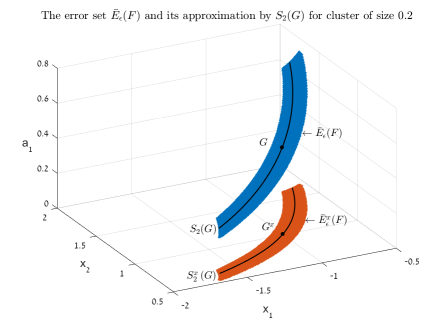
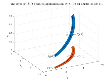
   Figure 1. The projections of the error set $\bar{E}_{\epsilon}(F)$ and a section of the Prony curve $S_{2}(G)$, for $F=\frac{1}{2}\delta\left(x+0.1\right)+\frac{1}{2}\delta\left(x-0.1\right)$, $h=0.1$, $\epsilon=h^{3}$ and $G=\Psi_{0,h}(F)$.

   

   Figure 2. The projections of the error set $\bar{E}_{\epsilon}(F)$ and a section of the Prony curve $S_{2}(G)$, for $F=\frac{1}{2}\delta\left(x+0.05\right)+\frac{1}{2}\delta\left(x-0.05\right)$, $h=0.05$, $\epsilon=h^{3}$ and $G=\Psi_{0,h}(F)$. Note the convergence of $\bar{E}_{\epsilon}(F)$ into $S_{2}(G)$ as the cluster size reduces.

2. In Section 6, Theorems 6.1 and 6.2, we use the above result to derive lower and upper bounds, of the same order, on the worst case reconstruction error. We show that:
   The worst case reconstruction error,

   $$\rho(F,\epsilon)=\max_{F^{\prime}\in E_{\epsilon}(F)}\|F^{\prime}-F\|,$$

   is of order $\epsilon h^{-2d+1}$.
   The worst case reconstruction error of the amplitudes,

   $$\rho_{a}(F,\epsilon)=\max_{F^{\prime}=(a^{\prime},x^{\prime})\in E_{\epsilon}(F)}\|a^{\prime}-a\|,$$

   is of order $\epsilon h^{-2d+1}$.
   The worst case reconstruction error of the nodes,

   $$\rho_{x}(F,\epsilon)=\max_{F^{\prime}=(a^{\prime},x^{\prime})\in E_{\epsilon}(F)}\|x^{\prime}-x\|,$$

   is of order $\epsilon h^{-2d+2}$.

   We stress that reconstructions $F^{\prime}$ with reconstruction errors as above cannot occur everywhere: they fall into a small neighborhood of the Prony curve $S_{2d-2}(F)$. This fact is used in Section 3 to improve the reconstruction accuracy (see item 4 below).

   Our next result concerns the accuracy of reconstruction of the Prony varieties $S_{q}(F)$:

3. While the point worst case reconstruction error of the signal $F$ is of order $\epsilon h^{-2d+1}$, the curve $S_{2d-2}(F)$ itself can be reconstructed with a better accuracy of order $\epsilon h^{-(2d-2)}$. The “hierarchy of the accuracy rates” is continued along the chain $S_{2d-1}(F)\subset\ldots\subset S_{0}(F)$ of the Prony varieties $S_{q}(F)$: each $S_{q}(F)$ can be reconstructed with an accuracy of order $\epsilon h^{-q}$. See Theorem 6.4.

   Based on the theory developed in sections 5 and 6 we conclude our results with the following fact:

4. If a certain additional a priori information is available on the signal $F$, the reconstruction accuracy can be significantly improved via the following procedure: first we reconstruct the Prony variety $S_{q}(F)$ for a certain appropriate $q$. The accuracy of this reconstruction (of order $\epsilon h^{-q}$) is higher than that of a single point solution. Then we use the additional information available in order to accurately localize the signal $F$ inside the Prony variety $S_{q}(F)$. In section 3 we demonstrate this procedure and how it can improve the reconstruction accuracy with respect to Prony method.

Remark 1.4.

Consider the case $\epsilon$ of order greater than $h^{2d-1}$. Our approach, based on the regularity of the moment coordinates, does not apply here since for large errors the reconstruction encounters singularities. We do not study this case here, however, the Prony varieties $S_{q}$, being algebraic objects that are defined globally, remain a relevant tool in studying error amplification and collision singularities in much larger scales (See [9, 16, 17]).

1.4. Organization of the text

In Section 2 we discuss related settings and results. In particular, we explain in detail the connection between the results of the resent paper to the case of Fourier measurements / super resolution setting (in particular, with $N\gg 2d$ or continuous samples), and the possible extensions to the case of several clusters.

In Section 3 we show possible applications of our results to improving the reconstruction accuracy of Prony method. We provide a simple example, supported by numerical simulations, where taking into account the Prony varieties, significantly improves the reconstruction accuracy.

Sections 4 - 6 are devoted to the accurate stating of the results and their proofs. In Section 4 we introduce the “Prony mapping”, and study its inversion via “Quantitative inverse function theorem”. In Section 5 our main results on the geometry of the error set are stated and proved. In Section 6 we derive, based on the previous section, tight estimates on the worst case reconstruction error. Finally, in Appendix (B), we proof a specific form of the quantitative inverse function theorem, giving explicit expression for the constants used in the text.

1.5. Acknowledgements

The research of GG and YY is supported in part by the Minerva Foundation. The authors would like to thank the referees for suggesting significant improvements in the presentation.

2. Related work and discussion

As it was already mentioned in the Introduction, in the present paper we concentrate on a rather restricted case of the spike-train reconstruction problem. First, we take the real moments as the measurements (instead of much more common and natural Fourier samples). Second, we take exactly $2d$ moment measurements (instead of $N\gg 2d$ moments or Fourier samples). Finally, we assume that the nodes of $F$ form exactly one cluster, instead of the more general configuration of several clusters.

The main reasons for us to insist on this setting is that it presents in a relatively compact form the most essential patterns of the error amplification in multi-cluster moment / Fourier spike-train reconstruction. We discuss this fact in detail in subsections 2.1, 2.2, 2.3 below.

2.1. Clustered Fourier reconstruction (super-resolution)

In this section we outline the tight connection between the super-resolution problem, where the measurements are Fourier samples, and the results of the present paper about moment reconstruction. In fact, up to constants, the error set in the case of Fourier measurements is described by exactly the same moment inequalities, as in the present paper.

For a signal $F$ of the form (1.1), let ${\mathcal{}{F}}\left(F\right)$ denote the Fourier transform of $F$:

$${\mathcal{}F}(F)(s)=\int_{-\infty}^{\infty}F(x)e^{-2\pi ixs}dx=\sum_{j=1}^{d}a_{j}e^{-2\pi ix_{j}s}.$$

In a super resolution setting, it is frequently assumed that the measurements for the reconstruction of $F$ are given as a function $\Phi$ satisfying

(2.1) $$\left|\Phi(s)-{\mathcal{}F}(F)(s)\right|\leq\epsilon,\quad s\in[-\Omega,\Omega].$$

where $\epsilon>0$ is the noise level and $\Omega>0$ is the band limit.

Similarly to the moment $\epsilon$-error set 1.1, we define the Fourier $\epsilon$-error set as follows.

Definition 2.1.

For $\epsilon,\Omega>0$ and $F\in{\mathcal{}P}_{d}$, the Fourier error set $E_{\epsilon,\Omega}(F)\subset{\mathcal{}P}_{d}$ is the set consisting of all the signals $F^{\prime}\in{\mathcal{}P}_{d}$ with

$$\left|{\mathcal{}F}(F^{\prime})(s)-{\mathcal{}F}(F)(s)\right|\leq\epsilon, s\in[-\Omega,\Omega].$$

Let $F$ form an $(h,\kappa,\eta,m,M)$-regular cluster as the case considered in this paper. Define the super resolution factor as

$$SRF=\frac{1}{\Omega h}.$$

The radius of the Fourier error set, or equivalently the worst case reconstruction error of $F$, in the super resolution setting (2.1), was shown to scale like $SRF^{2d-1}\epsilon$ (see [1, 7, 24] for off-grid setting and [12, 11, 5, 23] for on-grid setting). If we further assume that at most $l\leq d$ nodes of $F$ form a cluster of size $h$, then recent results show that the scaling of the radius of the error set improves to an order of $SRF^{2l-1}\epsilon$ (see [5, 23, 20, 7, 24, 21]).

The Fourier error set and the moment error set are related via the Taylor series expansion of the Fourier transform, that is expressed using the moments as follows (see [1, Proposition 3.1]):

(2.2) $${\mathcal{}F}(F)(s)=\sum_{k=0}^{\infty}{\frac{m_{k}(F)}{k!}}\tilde{s}^{k},\ \text{w}here\ \ \tilde{s}=-2\pi is.$$

In fact it is possible to show that these sets are equivalent in the following sense:

Let $F=(a,x)\in{\mathcal{}P}_{d}$ form an $(h,\kappa,\eta,m,M)$-regular cluster. Then, there exist positive constants $\Cl[B]{srf.low.equi},\Cl[B]{noise.up.equi}$ and $\Cl[B]{low.equi}\leq 1\leq\Cl[B]{high.equi}$, depending only on $\eta,d,m,$ such that for each $\Omega,\epsilon$ satisfying $SRF\geq\Cr{srf.low.equi}$ and $0\leq\epsilon\leq\Cr{noise.up.equi}(SRF)^{-2d+1}$, it holds that

(2.3) $$E_{\Cr{low.equi}\epsilon}(\Psi_{\kappa,\frac{1}{\Omega}}(F))\subseteq\Psi_{\kappa,\frac{1}{\Omega}}\big{(}E_{\epsilon,\Omega}(F)\big{)}\subseteq E_{\Cr{high.equi}\epsilon}(\Psi_{\kappa,\frac{1}{\Omega}}(F)),$$

or equivalently

(2.4) $$\Psi^{-1}_{\kappa,\frac{1}{\Omega}}\big{(}E_{\Cr{low.equi}\epsilon}(\Psi_{\kappa,\frac{1}{\Omega}}(F))\big{)}\subseteq E_{\epsilon,\Omega}(F)\subseteq\Psi^{-1}_{\kappa,\frac{1}{\Omega}}\big{(}E_{\Cr{high.equi}\epsilon}(\Psi_{\kappa,\frac{1}{\Omega}}(F))\big{)}.$$

Put differently, for a signal $F$ with clustered nodes as above, and for any signal $F_{1}\in{\mathcal{}P}_{d}$, the Fourier difference is $\epsilon$ small, i.e.

$$\max_{s\in[-\Omega,\Omega]}|{\mathcal{}F}(F_{1})(s)-{\mathcal{}F}(F)(s)|\leq\epsilon,$$

if and only if the moments $m_{0},\ldots,m_{2d-1}$, of the centered and scaled by $\Omega$ difference signal $\Psi_{\kappa,\frac{1}{\Omega}}(F)-\Psi_{\kappa,\frac{1}{\Omega}}(F_{1})$, are order of $\epsilon$ small.

The main result of this paper concerning the geometry of moment reconstruction (see Theorem 5.1 and Theorem 5.2) is extended to Fourier reconstruction via relation (2.3) (or relation (2.4)), as follows. See also Figure 3.

Corollary 2.1.

Let $F=(a,x)\in{\mathcal{}P}_{d}$ form an $(h,\kappa,\eta,m,M)$-regular cluster. Then, there exist positive constants $\Cl[B]{srf.low.cor.main},\Cl[B]{noise.cor.main},\Cl[B]{cor.main}$, depending only on $d,\eta,m,M$, such that for each $\Omega,\epsilon$ satisfying

$$SRF\geq\Cr{srf.low.cor.main}\mbox{\hskip 20.00003ptand \hskip 20.00003pt}0\leq\epsilon\leq\Cr{noise.cor.main}(SRF)^{-2d+1},$$

$E_{\epsilon,\Omega}(F)$ is contained within the $\Delta_{q}$-neighborhood of the Prony variety $S_{q}(F)$, for

$$\Delta_{q} =\Cr{cor.main}\left(SRF\right)^{q}\epsilon, q=0,\ldots,2d-1.$$

See proof of Corollary 2.1 in Appendix A.

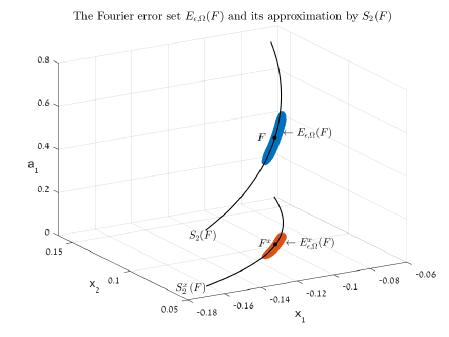
Figure 3. The projections of the Fourier error set $E_{\epsilon,\Omega}(F)$ and a section of the Prony curve $S_{2}(F)$, for $F=\frac{1}{2}\delta\left(x+0.1\right)+\frac{1}{2}\delta\left(x-0.1\right)$, $h=0.1$ and $\epsilon=5h^{3}$. Compare with Figure 2.

This geometrical structure of the Fourier error set suggests a similar procedure to improve the reconstruction accuracy, as we demonstrate for the Prony method, in Section 3. We intend to present results in this direction in future work.

Finally, using the equivalence relation (2.3) (or relation (2.4)), one can also derive the worst case reconstruction error rates for Fourier reconstruction of a signal cluster, based on the corresponding moment reconstruction error rates that we prove in Section 6, Theorem 6.1 and Theorem 6.2.

Corollary 2.2.

Let $F=(a,x)\in{\mathcal{}P}_{d}$ form an $(h,\kappa,\eta,m,M)$-regular cluster. Then, there exist positive constants $\Cl[B]{cor.worst.srf},\Cl[B]{cor.worst.noise}$, depending only on $d,\eta,m,M$, such that for each $\Omega,\epsilon$ satisfying

$$SRF\geq\Cr{cor.worst.srf}\mbox{\hskip 20.00003ptand \hskip 20.00003pt}0\leq\epsilon\leq\Cr{cor.worst.noise}(SRF)^{-2d+1},$$

It holds that:

(2.5) $$\max_{F^{\prime}\in E_{\epsilon,\Omega}(F)}\|F^{\prime}-F\| \asymp SRF^{2d-1}\epsilon,$$

(2.6) $$\max_{F^{\prime}=(a^{\prime},x^{\prime})\in E_{\epsilon,\Omega}(F)}\|a^{\prime}-a\| \asymp SRF^{2d-1}\epsilon,$$

(2.7) $$\max_{F^{\prime}=(a^{\prime},x^{\prime})\in E_{\epsilon,\Omega}(F)}\|x^{\prime}-x\| \asymp SRF^{2d-1}h\epsilon.$$

See proof of Corollary 2.2 in Appendix A.

2.2. More measurements

In the present paper, we keep the number of moment measurements exactly $2d$: this is enough to obtain the correct error asymptotic behavior for the cluster size $h\ll 1$.

However, the results of this paper can be used in order to accurately estimate the worst case reconstruction error / minimax error rate in multi-cluster super resolution setting. This is done in [7], in the following main steps:

1. Let $F=\sum_{j=1}^{d}a_{j}\delta(x-x_{j}),\ a_{j}\in{\mathbb{C}},\ x_{j}\in{\mathbb{R}}$. We apply “decimation” (see [4]), i.e. take exactly $2d$ uniformly spaced Fourier samples, with the step-size $\lambda$ of order $\frac{\Omega}{2d}$. In other words, we use “most of the available bandwidth $\Omega$”, keeping the number of the samples $2d$. As a result we get a Prony system with the nodes $z_{j}=e^{2\pi i\lambda x_{j}}$ on the unit circle. Clearly, the size $h$ of any cluster becomes $\lambda h\sim\Omega h$.

2. We show that for “many” values of $\lambda$ no new proximities between the nodes on the circle are created.

3. We apply the approach of the present paper (but with the “quantitative inverse function theorem” extended to the complex spaces), and finally produce the accuracy bounds of the required form, with $h$ replaced by $\Omega h$ (see Section 2.1). This gives a “correct” decay rate of the reconstruction error, with respect to the bandwidth $\Omega$.

Available studies of certain high-resolution algorithms such as MUSIC [25], ESPRIT/Matrix Pencil [13], Approximate Prony Method [30], multivariate Prony method [19] and others provide rigorous performance guarantees for the case $SRF<1$. We hope that our proof techniques here and in [7] may be used in deriving the stability limits of these and other methods in the super-resolution regime, i.e. for $SRF>1$.

2.3. The case of several clusters

Our description of the error set, via the moment inequalities, and of its “skeleton”, provided by the hierarchy of the Prony varieties, extends to spike train signals forming several clusters. Let $F$ be a signal with the node clusters $Q_{1},\ldots,Q_{m}$, each $Q_{s}$ being of size $h_{s}$ and containing $d_{s}$ nodes, $s=1,\ldots,m$. Denote by $F_{s}$ the “local signals”, corresponding to the clusters $Q_{s}$. The main fact in this situation is the following:

If the clusters $Q_{s}$ of $F$ are “well-separated”, in comparison to their size, then the error set of $F$ is, essentially, the Cartesian product of the “local” error sets of $F_{s},\ s=1,\ldots,m$. This up to constants, depending on the mutual position of the clusters $Q_{s}$, on their “multiplicities” $d_{s}$, and on their sizes $h_{s}$.

This claim follows from the “mutual independence” of the local signals $F_{s}$, corresponding to the node clusters $Q_{s}$:

The errors in the moments of the local signals $F_{s}$ cannot cancel in the moments of their sum $F$.

This last property is important in many questions far beyond the study of multi-cluster error sets and Prony varieties. Through the Jacobian of the Prony mapping it is closely connected with the properties of Vandermonde matrices with clustered nodes. Recently we’ve shown in [6] that the column subspaces of the clusters of a rectangular Vandermonde matrix are near-orthogonal, for the parameters in a “correct range”. This result strongly supports the “mutual independence” of the local signals $F_{s}$, corresponding to the node clusters $Q_{s}$.

Consequently, also the description of the error set using the Prony varieties, given in the present paper for one cluster, extends to the multi-cluster case via the Cartesian products of the local Prony varieties as follows: For each $q$, consider the subvariety $\tilde{S}_{q}$ in the signal space, which is the Cartesian product of the “local” Prony varieties $S_{q}^{s}$ corresponding to the clusters $Q_{s}$:

$$\tilde{S}_{q}=S^{1}_{q}\times S^{2}_{q}\times\ldots\times S^{m}_{q}.$$

We see immediately that the moments up to $q$ are constant on $\tilde{S}_{q}$, while the higher moments $m_{k}$ can be locally bounded through the $k$-th powers of the cluster sizes $h_{s}$. Consequently, $\tilde{S}_{q}$ play in the multi-cluster case the same role of a “skeleton” of the error set, as $S_{q}$ in the case of one cluster, described in detail in the present paper.

Thus, in principle, the main results of the current paper can be extended to several clusters. However, technically, the accurate description becomes rather involved. Still, we believe that a detailed understanding of the “algebraic-geometric skeleton” of the error amplification in the case of several clusters is highly important. We plan to present results in this direction separately.

3. Improving the reconstruction accuracy given some additional information

In this section we shortly discuss the way one can use the Prony varieties in order to improve the reconstruction accuracy of a spike train signal from its $2d$ initial moments. Specifically, we show that Prony varieties can help to optimally utilize an additional information on the reconstructed signals.

As we explain in Section 2.1, the spreading and scale of the error in Fourier reconstruction is tightly connected to moment reconstruction via (2.4) (see also Figure 3). We therefore expect that the procedure we describe here can ultimately help to improve the accuracy of widely used Fourier reconstruction methods - ESPRIT, APM, Matrix pencil and variants. We intend to present results in this direction in future separate work.

Assume that the measured signal $F$, is known to form a small regular cluster of size $h\ll 1$. Assume in addition that we have certain additional information on the signal $F$. We do not specify here the nature of this information, which can either be known a priori or a result of a different, non-moment, measurement of the signal, assuming just that the measured signal is known to reside within a subset $\Omega\subset{\mathcal{}P}$.

Recall that for measurement error $\epsilon\geq 0$, our input for the reconstruction of $F$ are the moment measurements $\mu^{\prime}=(\mu^{\prime}_{0},\ldots,\mu^{\prime}_{2d-1})$ with

(3.1) $$|\mu_{k}^{\prime}-m_{k}(F)|\leq\epsilon,\hskip 20.00003ptk=0,1,\ldots,2d-1.$$

Now consider the following reconstruction procedure:

Input : number of nodes $d$.

Input : measured moments $\mu^{\prime}=(\mu^{\prime}_{0},\ldots,\mu^{\prime}_{2d-1})$ satisfying (3.1).

Input : feasible set $\Omega\subset{\mathcal{}P}_{d}$.

Output : an estimate $F^{PCRP}\in{\mathcal{}P}_{d}$.

1 Solve the Prony system (3.1) with input $\mu^{\prime}$ and recover the signal $F^{\prime}$;

2 Use $F^{\prime}$ to reconstruct the Prony curve $S_{2d-1}(F^{\prime})$;

3 if $S_{2d-1}(F^{\prime})\cap\Omega\neq\emptyset$ then

4       Find a signal $F^{PCRP}$ which is closest to $F^{\prime}$ in the intersection $S_{2d-1}(F^{\prime})\cap\Omega$, i.e.

$$F^{PCRP}=\operatorname*{arg\,min}_{F\in S_{2d-1}(F^{\prime})\cap\Omega}\|F^{\prime}-F\|;$$

return the estimate $F^{PCRP}$.

5else

6       Find a signal $F^{SRP}$ which is closest to $F^{\prime}$ in the feasible set $\Omega$, i.e.

$$F^{SRP}=\operatorname*{arg\,min}_{F\in\Omega}\|F^{\prime}-F\|;$$

return the estimate $F^{SRP}$.

Algorithm 3.1 Prony curve reconstruction procedure given a priori information - PCRP

We compare the above procedure to the following “natural” solution algorithm using Prony method, which does not relies on Prony curves (and appears as an edge case of the PCRP in step 6):

Input : number of nodes $d$.

Input : measured moments $\mu^{\prime}=(\mu^{\prime}_{0},\ldots,\mu^{\prime}_{2d-1})$ satisfying (3.1).

Input : feasible set $\Omega\subset{\mathcal{}P}_{d}$.

Output : an estimate $F^{SRP}\in{\mathcal{}P}_{d}$.

1 Solve the Prony system (3.1) with input $\mu^{\prime}$ and recover the signal $F^{\prime}$;

Find a signal $F^{SRP}$ which is closest to $F^{\prime}$ in the feasible set $\Omega$, i.e.

$$F^{SRP}=\operatorname*{arg\,min}_{F\in\Omega}\|F^{\prime}-F\|;$$

return the estimate $F^{SRP}$.

Algorithm 3.2 Standard reconstruction procedure given a priori information- SRP

Let us now explain why the reconstruction procedure using the Prony curve, PRCP, is expected to improve the accuracy with respect to standard reconstruction procedure, SRP, of solving the Prony system and then projecting the solution into the feasible set.

Consider the solution $F^{\prime}$ to the Prony system (3.1), with input $\mu^{\prime}$, appearing as a first step in both reconstruction procedures. The distance of $F^{\prime}$ from $F$, in the worst case, is of order $h^{-2d+1}\epsilon$ (see item 2 in the sketch of the main results or the formal result in Theorem 6.2). We have that the true solution $F$ is contained in an order of $h^{-2d+2}\epsilon$ neighborhood of the Prony curve $S_{2d-1}(F^{\prime})$ (see item 3 in the sketch of the main results or the formal result in Corollary 6.2).

At the final step of the SRP we take the closest signal to $F^{\prime}$ in $\Omega$. This closest point is typically at the same distance of order $h^{-2d+1}\epsilon$ from $F$. In contrast, in the PCRP we take the closest signal to $F^{\prime}$ in $\tilde{\Omega}=S_{2d-1}(F^{\prime})\cap\Omega$ (presuming that this set is non-empty, see step 4 in the PCRP). Now since $F$ is located in a tiny belt around $S_{2d-1}(F^{\prime})$, and provided that the diameter of $\tilde{\Omega}$ is of order $h^{-2d+2}\epsilon$ or less, we get an order of $h$-magnitude better accuracy guarantees compared to the SRP. That is, in such case we get that the worst case reconstruction error of the PCRP is $\sim h^{-2d+2}\epsilon$, while the worst case reconstruction error of the SRP is $\sim h^{-2d+1}\epsilon$.

The same explanation as above holds for comparing the reconstruction accuracy of the nodes of $F$, but with all accuracy bounds multiplied by $h$. That is, if the diameter of the projection of $\tilde{\Omega}$ into the nodes coordinates is $\sim h^{-2d+3}\epsilon$, then the worst case reconstruction error of the nodes using the PCRP is $\sim h^{-2d+3}\epsilon$, whereas the worst case reconstruction error using the SRP is $\sim h^{-2d+2}\epsilon$.

In Figure 4 we demonstrate this effect on the reconstruction of the nodes of $F$.

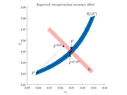
Figure 4. Above $F=\frac{1}{2}\delta(x+0.05)+\frac{1}{2}\delta(x-0.05)$ and $\epsilon=h^{3}$. $F^{\prime}$ is the reconstruction from the measurements $\mu^{\prime}=(1,0,h^{2},-h^{3})$. In blue is the $\epsilon$-error set. Note the improved reconstruction $F^{PCRP}$ attained by moving over the Prony curve, compared to $F^{SRP}$.

3.1. Numerical experiments

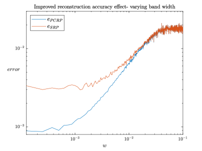
Figure 5.

Figure 5 shows the results of our numerical experiments which are arranged as follows: We fix the signal $F=\frac{1}{2}\delta(x+0.05)+\frac{1}{2}\delta(x-0.05)$ and a noise level of $\epsilon=h^{3}=(0.1/2)^{3}$. The feasible sets $\Omega^{x}_{w}$ in the node space are the strips transversal to $S_{2d-1}(F)$,

$$\Omega^{x}_{w}=\{(x_{1},x_{2}),\ |x_{1}+x_{2}|\leq w\}$$

(as seen in Figure 4, highlighted in pink). For uniform $\epsilon$-noise (i.e. the measured moments are uniformly distributed inside the $\epsilon$-cube in the moments space), we plot the averages $e_{SRP},e_{PCRP}$ of the reconstruction error of the two procedures as a function of the width $w$ of $\Omega^{x}_{w}$.

As seen in the figure, the advantage of the PCRP grows as the size $w$ decreases. For values of $w\sim h^{2}$ or less the $PCRP$ attains a reconstruction error of $\sim h^{2}$ while the $SRP$ attains a reconstruction error of $\sim h$.

4. Prony mapping and its inversion

4.1. Prony mapping

Definition 4.1.

The Prony mapping $PM=PM_{d}:{\mathcal{}P}_{d}\to{\mathcal{}M}_{d}$ is given by

$$PM(F)=\mu=(\mu_{0},\ldots,\mu_{2d-1})\in{\mathcal{}M},\ \mu_{k}=m_{k}(F),\ k=0,\ldots,2d-1.$$

For $F\in{\mathcal{}P}$ the problem of its reconstruction from the exact moment measurements $\mu=(\mu_{0},\ldots,\allowbreak\mu_{2d-1})\in{\mathcal{}M},$ is the problem of inverting the Prony mapping $PM.$ In this paper we always assume that this inversion (when defined) is accurate.

Consider the noisy measurements $\mu^{\prime}=(\mu^{\prime}_{0},\ldots,\mu^{\prime}_{2d-1})\in{\mathcal{}M}$ of the moments of $F$. By our assumption, the measurement error of each of the moments $m_{k}(F)$ does not exceed $\epsilon$, i.e. $|\mu^{\prime}_{k}-\mu_{k}(F)|\leq\epsilon$. Equivalently, the noisy measurement $\mu^{\prime}$ may fall at any point in the cube

(4.1) $$Q_{\epsilon}(\mu)=\{\mu^{\prime}=(\mu^{\prime}_{0},\ldots,\mu^{\prime}_{2d-1})\in{\mathcal{}M},\ |\mu^{\prime}_{k}-\mu_{k}|\leq\epsilon,\ k=0,1,\ldots,2d-1\}.$$

Consequently, the $\epsilon$-error set $E_{\epsilon}(F)$ is the preimage $PM^{-1}(Q_{\epsilon}(\mu))\subset{\mathcal{}P}.$

4.2. Inverse Function theorem and its consequences

Our first result describes the inversion of the Prony mapping in a neighborhood of a “regular point”, i.e. of a signal $G$ with all its $d$ nodes well separated, and with all its amplitudes bounded and well separated from zero. This result is, essentially, a direct application of the “quantitative inverse function theorem” (see, for instance, [18], page 264, Theorem 2.10.7 or [14], Theorem 3.2) combined with the estimates of the norm of the Jacobian of the Prony mapping and the norm of its inverse.

Assume that the nodes $x_{1},\ldots,x_{d}$ of a signal $G$ all belong to the interval $I=[-1,1]$, and for a certain $\eta$ with $0<\eta\leq\frac{2}{d-1}$, $d>1$, the distance between the neighboring nodes $x_{j},x_{j+1},\ j=1,\ldots,d-1,$ is at least $\eta$. We also assume that for certain $m,M$ with $0<m<M$, the amplitudes $a_{1},\ldots,a_{d}$ satisfy $m\leq|a_{j}|\leq M,\ j=1,\ldots,d$. We call such signals $(\eta,m,M)$-regular. We distinguish (as above) the parameter and the moment spaces of the model signals $G$, denoting them by $\bar{\mathcal{}P},\bar{\mathcal{}M},$ respectively. For $G\in\bar{\mathcal{}P}$ we denote by $\nu=(\nu_{1},\ldots,\nu_{2d-1})$ its Prony image $PM(G)\in\bar{{\mathcal{}M}}.$

For a matrix $B=[b_{ij}]$, we denote by $\|B\|$ its maximum norm:

$$\|B\|=\max_{i}{\sum_{j}|b_{ij}|}.$$

Theorem 4.1.

Let $G$ be an $(\eta,m,M)$-regular signal then there exist positive constants $R,C_{1},\allowbreak C_{2},C_{3},C_{4}$ (given explicitly below and in Appendix B) depending only on $d,\eta,m,M$ such that

1. The Jacobian $J$ at $G$ of the Prony mapping $PM$ is invertible, with

   $$\|J^{-1}\|\leq C_{1},\|J\|\leq C_{2}.$$

2. The inverse mapping $PM^{-1}$ exits on the cube $Q_{R}(\nu)$ of size $R$ centered at $\nu\in\bar{\mathcal{}M},$ and provides a diffeomorphism of $Q_{R}(\nu)$ to $\Omega_{R}(G)=PM^{-1}(Q_{R}(\nu))$. For each $\nu^{\prime},\nu^{\prime\prime}\in Q_{R}(\nu)$

   $$C_{3}\|\nu^{\prime\prime}-\nu^{\prime}\|\leq\|PM^{-1}(\nu^{\prime\prime})-PM^{-1}(\nu^{\prime})\|\leq C_{4}\|\nu^{\prime\prime}-\nu^{\prime}\|.$$

Proof.

Let $J=J(G)$ denote the Jacobian matrix of $PM$ at a (regular) signal $G$,

$$J_{k,j}=\begin{cases}\frac{\partial m_{k}(G)}{\partial a_{j}}=x_{j}^{k},&k=0,\ldots,2d-1,\hskip 20.00003ptj=1,\ldots,d,\\ \frac{\partial m_{k}(G)}{\partial x_{j}}=ka_{j}x_{j}^{k-1},&k=0,\ldots,2d-1,\hskip 20.00003ptj=d+1,\ldots,2d.\\ \end{cases}$$

The matrix $J$ admits the following factorization (about factorization of the Prony Jacobian see also [8])

(4.2) $$J=\begin{bmatrix}1&..&1&0&..&0\\ x_{1}&..&x_{d}&1&..&1\\ .&..&.&.&..&.\\ x_{1}^{2d-1}&..&x_{d}^{2d-1}&(2d-1)x_{1}^{2d-2}&..&(2d-1)x_{d}^{2d-2}\end{bmatrix}\begin{bmatrix}I_{d}&0\\ 0&D\end{bmatrix},$$

where $D=diag(a_{1},\ldots,a_{d})$ is a $d\times d$ diagonal matrix with the amplitudes on the diagonal and $I_{d}$ is the $d\times d$ identity matrix. Denote the left hand matrix in this factorization by $U_{2d}$. This is a special type of a confluent Vandermonde matrix, the norm of its inverse, which is important in our estimates, was studied in [15].

Theorem 4.2 (Gautschi, [15], Theorem 3).

$$\|U_{2d}^{-1}\|\leq\max_{1\leq\lambda\leq d}\;b_{\lambda}\left(\prod_{j=1,j\neq\lambda}^{d}\frac{1+|x_{j}|}{|x_{\lambda}-x_{j}|}\right)^{2},$$

$$b_{\lambda}=\max\left[1+|x_{\lambda}|,1+2(1+|x_{\lambda}|)\sum_{j=1,j\neq\lambda}^{d}\frac{1}{|x_{\lambda}-x_{j}|}\right].$$

Based on the above, for $U_{2d}$ formed by the nodes of an $(\eta,m,M)$-regular signal, that is $|x_{i}|\leq 1$ and $|x_{i}-x_{j}|\geq\eta$, it is straight forward to bound $\|U_{2d}^{-1}\|$ in terms of the constants $\eta,d$. The following proposition (given without proof) provide such upper bound.

Proposition 4.1.

Let $|x_{i}|\leq 1$ and $|x_{i}-x_{j}|\geq\eta$ then

$$\|U_{2d}^{-1}\|\leq(1+4\eta^{-1}(\ln(d)+1))\left(\frac{\eta^{-d+1}2^{d-1}}{\left(\lfloor\frac{d-1}{2}\rfloor!\right)^{2}}\right)^{2}.$$

Now using proposition 4.1 and the factorization equation (4.2) we have that

(4.3) $$\|J^{-1}\|\leq\max[1,m^{-1}](1+4\eta^{-1}(\ln(d)+1))\left(\frac{\eta^{-d+1}2^{d-1}}{\left(\lfloor\frac{d-1}{2}\rfloor!\right)^{2}}\right)^{2}=C_{1}(m,\eta,d)=C_{1}.$$

In addition, for an $(\eta,m,M)$-regular signal, a direct calculation shows that

$$\|J\|\leq d+M(2d-1)d=C_{2}.$$

This conclude the proof of statement 1 of Theorem 4.1.

The second statement of Theorem 4.1 follows from “quantitative inverse function theorem” (see, [18], Theorem 2.10.7 or [14]) taking into account that in this result the constants $C_{3},C_{4}$ and $R$ are given in terms of upper bounds on $\|J^{-1}\|,\|J\|$ and a local upper bound on the magnitude of the second derivatives of $PM$. The latter can be easily obtained in terms of $d,\eta,m,M$. The required constants $C_{3},C_{4}$ and $R$ are derived explicitly in appendix B. This completes the proof of Theorem 4.1. ∎

Let us denote $\Omega_{R}(G)\subset\bar{\mathcal{}P}$ as the preimage $PM^{-1}(Q_{R}(\nu))$. We give an equivalent formulation of Theorem 4.1, in terms of the moment coordinates.

Definition 4.2.

For $G$ a regular signal as above, and $G^{\prime}$ denoting signals near $G$, the moment coordinates are the functions $f_{k}(G^{\prime})=m_{k}(G^{\prime})-m_{k}(G),\;k=0,...,2d-1$. The moment metric $d(G^{\prime},G^{\prime\prime})$ on $\bar{\mathcal{}P}$ is defined through the moment coordinates as

$$d(G^{\prime},G^{\prime\prime}):=\max_{k=0}^{2d-1}|m_{k}(G^{\prime\prime})-m_{k}(G^{\prime})|=\|PM(G^{\prime})-PM(G^{\prime\prime})\|.$$

Corollary 4.1.

Let $G$ be a regular signal as above. Then the moment coordinates form a regular analytic coordinate system on $\Omega_{R}(G)$. The moment metric $d(G^{\prime},G^{\prime\prime})$ is bi-Lipschitz equivalent on $\Omega_{R}(G)$ to the maximum metric   $\|G^{\prime\prime}-G^{\prime}\|$ in $\bar{\mathcal{}{P}}$:

$$C_{3}d(G^{\prime},G^{\prime\prime})\leq\|G^{\prime\prime}-G^{\prime}\|\leq C_{4}d(G^{\prime},G^{\prime\prime}).$$

Proof.

It follows directly from Theorem 4.1. ∎

5. The geometry of the error set for nodes forming an $h$-cluster

We use regular signals $G$ as above, as a model for signals with a “regular cluster”: For $F\in{\mathcal{}P}$ with $h=h(F)$ and $\kappa=\kappa(F)$ (i.e. $F$ having its nodes cluster in an interval of size $h$ and center $\kappa$), we say that $F$ forms an $(h,\kappa,\eta,m,M)$-regular cluster if $G=\Psi_{\kappa,h}(F)$ is an $(\eta,m,M)$-regular signal. Explicitly $F$ forms an $(h,\kappa,\eta,m,M)$-regular cluster if its amplitudes $a_{1},\ldots,a_{d}$ satisfy $m\leq|a_{j}|\leq M,\ j=1,\ldots,d,$ and the distance between the neighboring nodes $x_{j},x_{j+1},\ j=1,\ldots,d-1,$ is at least $\eta h$. We formulate our main results in terms of the model signal $G$.

For any $G\in\bar{{\mathcal{}P}}$ and $\epsilon,\alpha>0$ we define the following geometric objects:

Definition 5.1.

Define $\Pi_{\epsilon,\alpha}(G)\subset\bar{{\mathcal{}P}}$ as the parallelepiped, in moments coordinates, consisting of all signals $G^{\prime}\in\bar{\mathcal{}P}$ satisfying the inequalities

$$|m_{k}(G^{\prime})-m_{k}(G)|\leq\epsilon\alpha^{k},\ k=0,\ldots,2d-1.$$

Definition 5.2.

For each $0\leq q\leq 2d-1$, define $S_{q,\epsilon,\alpha}(G)$ as the part of the Prony variety $S_{q}(G),$ consisting of all signals $G^{\prime}\in S_{q}(G)$ with

$$|m_{k}(G^{\prime})-m_{k}(G)|\leq\epsilon\alpha^{k},\ k=q+1,\ldots,2d-1.$$

5.1. The case of a zero shift

Theorem 5.1 below describes the set $\bar{E}_{\epsilon}(F)\subset\bar{\mathcal{}P}$, under an additional assumption that there is no shift. In this case the description becomes especially transparent. The effect of a non-zero shift $\kappa$ is described in Section 5.2 below. In particular, a version of Theorem 5.1 with a non-zero shift is given in Theorem 5.2.

Theorem 5.1.

Let $F\in{\mathcal{}P}$ form an $(h,0,\eta,m,M)$-regular cluster and let $G=\Psi_{0,h}(F)$ be the model signal for $F$. Then:

1. For each positive $\epsilon$ we have

   $$\bar{E}_{\epsilon}(F)=\Pi_{\epsilon,\frac{1}{h}}(G).$$

2. For each positive $\epsilon\leq Rh^{2d-1}$, $\bar{E}_{\epsilon}(F)$ is contained within the $\Delta_{q}$-neighborhood of the part of the Prony variety $S_{q,\epsilon,\frac{1}{h}}(G)$, for

   $$\Delta_{q}=C_{4}\left(\frac{1}{h}\right)^{q}\epsilon.$$

   The constants $R,C_{4}$ are defined in Theorem 4.1 above.

Remark 5.1.

Assume that the measurement error $\epsilon\leq Rh^{2d-1}$. By Corollary 4.1 we have that the metric induced by the moments is equivalent to maximum metric on $\bar{{\mathcal{}P}}$. Combing this with statement 1 of Theorem 5.1, we obtain that the error set $\bar{E}_{\epsilon}(F)$ is a “deformed” parallelepiped in standard coordinates of $\bar{{\mathcal{}P}}$. See figures 2 and 2 in subsection 1.3.

Proof of Theorem 5.1..

Denote by $M\bar{E}_{\epsilon}(F)=PM(\bar{E}_{\epsilon}(F))\subset\bar{\mathcal{}M}$ the set of all the possible errors in the moments $m_{k}(G),\ k=0,1,\ldots,2d-1,$ corresponding to the errors not exceeding $\epsilon$ in the moments of $F$.

Consider the scaling transformation $SC_{\alpha},$ which acts on signals $F$ via scaling of the nodes of $F$: $SC_{\alpha}(F)(x)=\frac{1}{\alpha}F(\frac{x}{\alpha}).$ For $F(x)=\sum_{j=1}^{d}a_{j}\delta\left(x-x_{j}\right)$ we have that $SC_{\alpha}(F)=\sum_{j=1}^{d}a_{j}\delta\left(x-\alpha x_{j}\right),$ and therefore

(5.1) $$m_{k}(SC_{\alpha}(F))=\sum_{j=1}^{d}a_{j}\alpha^{k}x^{k}_{j}=\alpha^{k}m_{k}(F).$$

Accordingly, we define the scaling transformation $SC^{*}_{\alpha}:{\mathcal{}M}\to{\mathcal{}M}$ on the moment space as follows: for $\mu=(\mu_{0},\ldots,\mu_{2d-1})$

(5.2) $$SC^{*}_{\alpha}(\mu)=\nu=(\nu_{0},\ldots,\nu_{2d-1}),\ \nu_{k}=\alpha^{k}\mu_{k},\ k=0,\ldots,2d-1.$$

With these definitions we have for all $F^{\prime}\in{\mathcal{}P}$

(5.3) $$PM(SC_{\alpha}(F^{\prime}))=SC^{*}_{\alpha}(PM(F^{\prime})).$$

For the model signal $G$ we have $G=SC_{\frac{1}{h}}(F)$. Set $\mu=PM(F)$. Accordingly, the set $M\bar{E}_{\epsilon}(F)$ of the possible measurements for the moments of $G$ is $SC^{*}_{\frac{1}{h}}(Q_{\epsilon}(\mu)).$ The initial moment error set $E_{\epsilon}(F)$ is the $\epsilon$-cube $Q_{\epsilon}(\mu)$,

$$Q_{\epsilon}(\mu)=\{\mu^{\prime}=(\mu^{\prime}_{0},\ldots,\mu^{\prime}_{2d-1})\in{\mathcal{}M},\ |\mu^{\prime}_{k}-\mu_{k}|\leq\epsilon,\ k=0,1,\ldots,2d-1\}.$$

Consequently, $M\bar{E}_{\epsilon}(F)$ is a coordinate parallelepiped

(5.4) $$M\Pi_{\epsilon,\frac{1}{h}}(\nu):=\{\nu^{\prime}\in{\mathcal{}M},|\nu^{\prime}_{k}-\nu_{k}|\leq\epsilon\left(\frac{1}{h}\right)^{k},\ k=0,1,\ldots,2d-1\}.$$

The error set $\bar{E}_{\epsilon}(F)\subset\bar{\mathcal{}P}$ is the preimage

$$\bar{E}_{\epsilon}(F)=PM^{-1}(M\bar{E}_{\epsilon}(F))=PM^{-1}(M\Pi_{\epsilon,\frac{1}{h}}(\nu))=\Pi_{\epsilon,\frac{1}{h}}(G).$$

This concludes the proof of the first part of Theorem 5.1.

We now prove the second part of Theorem 5.1. By part one of the theorem we already know that $M\bar{E}_{\epsilon}(F)=M\Pi_{\epsilon,\frac{1}{h}}(\nu)$ is the parallelepiped given in (5.4). On the other hand $PM(S_{q,\epsilon,\frac{1}{h}}(G))$ is the projection of $M\Pi_{\epsilon,\frac{1}{h}}(\nu)$ into the last $2d-q-1$ coordinates (in the moments coordinate system centered at $G$). Hence

$$\max_{\nu^{\prime}\in M\bar{E}_{\epsilon}(F)}\min_{\nu^{\prime\prime}\in PM(S_{q,\epsilon,\frac{1}{h}}(G))}\|\nu^{\prime}-\nu^{\prime\prime}\|=\left(\frac{1}{h}\right)^{q}\epsilon.$$

In order to apply Theorem 4.1 and Corollary 4.1 we have to check that the parallelepiped $M\bar{E}_{\epsilon}(F)=M\Pi_{\epsilon,\frac{1}{h}}(\nu)$ is contained in the cube $Q_{R}(\nu)$ of size $R$ centered at $\nu\in\bar{\mathcal{}M}.$ The maximal edge of $M\Pi_{\epsilon,\frac{1}{h}}(\nu)$ has length $\epsilon h^{-2d+1}$, and hence for $\epsilon\leq Rh^{2d-1}$ the required inclusion holds. Now, by applying Corollary 4.1, we get

$$\max_{G^{\prime}\in\bar{E}_{\epsilon}(F)}\min_{G^{\prime\prime}\in S_{q,\epsilon,\frac{1}{h}}(G)}\|G^{\prime}-G^{\prime\prime}\|=C_{4}\left(\frac{1}{h}\right)^{q}\epsilon.$$

∎

5.2. The case of a non-zero shift

For a signal $G\in\bar{{\mathcal{}P}}$ recall that the parallelepiped $\Pi_{\epsilon,\alpha}(G)\subset\bar{{\mathcal{}P}}$, is the set of all signals $G^{\prime}\in\bar{\mathcal{}P}$ satisfying

$$|m_{k}(G^{\prime})-m_{k}(G)|\leq\epsilon\alpha^{k},\ k=0,\ldots,2d-1.$$

Theorem 5.2.

Let $F\in{\mathcal{}P}$ form an $(h,\kappa,\eta,m,M)$-regular cluster and let $G=\Psi_{\kappa,h}(F)$ be the model signal for $F$. Set $\epsilon^{\prime}=(1+|\kappa|)^{-2d+1}\epsilon$ and $h^{\prime}=\frac{h}{1+|\kappa|}$. Then:

1. For any $\epsilon>0$, the error set $\bar{E}_{\epsilon}(F)$ is contained between the following two parallelepipeds in the moment coordinates:

   $$\Pi_{\epsilon^{\prime},\frac{1}{h}}(G)\subset\bar{E}_{\epsilon}(F)\subset\Pi_{\epsilon,\frac{1}{h^{\prime}}}(G),$$

   where

   $$\Pi_{\epsilon^{\prime},\frac{1}{h}}(G) =\left\{G^{\prime}\in\bar{{\mathcal{}P}}:|m_{k}(G)-m_{k}(G^{\prime})|\leq(1+|\kappa|)^{-2d+1}\epsilon\left(\frac{1}{h}\right)^{k},\;k=0,\ldots,2d-1\right\},$$

   $$\Pi_{\epsilon,\frac{1}{h^{\prime}}}(G) =\left\{G^{\prime}\in\bar{{\mathcal{}P}}:|m_{k}(G)-m_{k}(G^{\prime})|\leq\epsilon\left(\frac{1+|\kappa|}{h}\right)^{k},\;k=0,\ldots,2d-1\right\}.$$

2. For any $\epsilon\leq Rh^{\prime 2d-1}$, the error set $\bar{E}_{\epsilon}(F)$ is contained within the $\Delta^{\prime}_{q}$-neighborhood of the part of the Prony variety $S_{q,\epsilon,\frac{1}{h^{\prime}}}(G)$, for

   $$\Delta^{\prime}_{q}=C_{4}\left(\frac{1}{h^{\prime}}\right)^{q}\epsilon.$$

   The constants $R,C_{4}$ are defined in Theorem 4.1 above.

Proof Theorem 5.2:.

Let us describe the effect of a shift transformation in ${\mathcal{}P}$ and in ${\mathcal{}M}$. Define the shift transformation $SH_{\kappa}:{\mathcal{}P}\to{\mathcal{}P}$ of the parameter space by $SH_{\kappa}(F)(x)=F(x+\kappa)$. The following proposition describes the action of the coordinate shift on the moments of general spike-trains:

Proposition 5.1.

$$m_{k}(F)=\sum_{l=0}^{k}\binom{k}{l}(\kappa)^{k-l}m_{l}(SH_{\kappa}(F)),\ m_{k}(SH_{\kappa}(F))=\sum_{l=0}^{k}\binom{k}{l}(-\kappa)^{k-l}m_{l}(F).$$

Proof.

For $F(x)=\sum_{j=1}^{d}a_{j}\delta(x-x_{j})\in{\mathcal{}P}$ we get

$$m_{k}(SH_{\kappa}(F))=\sum_{j=1}^{d}a_{j}(x_{j}-\kappa)^{k}=\sum_{j=1}^{d}a_{j}\sum_{l=0}^{k}\binom{k}{l}(-\kappa)^{k-l}x_{j}^{l}=$$

$$=\sum_{l=0}^{k}\binom{k}{l}(-\kappa)^{k-l}\sum_{j=1}^{d}a_{j}x_{j}^{l}=\sum_{l=0}^{k}\binom{k}{l}(-\kappa)^{k-l}m_{l}(F).$$

Replacing $\kappa$ by $-\kappa$ we get the second expression. ∎

Accordingly, we define the shift transformation $SH^{*}_{\kappa}:{\mathcal{}M}\to{\mathcal{}M}$ as the following linear transformation on the moment space: For $\mu^{\prime}=(\mu^{\prime}_{0},\ldots,\mu^{\prime}_{2d-1})\in{\mathcal{}M}$

$$SH^{*}_{\kappa}(\mu^{\prime})=\nu=(\nu_{0},\ldots,\nu_{2d-1}),\ \nu_{k}=\sum_{l=0}^{k}\binom{k}{l}(-\kappa)^{k-l}\mu_{l},\ k=0,1,\ldots,2d-1.$$

Proposition 5.1 shows that the shift transformations $SH_{\kappa}$ and $SH^{*}_{\kappa}$, and the Prony mapping $PM$ satisfy the following identity:

(5.5) $$PM(SH_{\kappa}(F))=SH^{*}_{\kappa}(PM(F)).$$

Since $SH^{*}_{\kappa}$ is a linear transformation we will omit the parentheses and write $SH^{*}_{\kappa}\mu$ instead of $SH^{*}_{\kappa}(\mu)$. We extend this rule to every linear transformation $T$ and write $Tv$ instead of $T(v)$. We have the following bounds for the norms of $SH^{*}_{\kappa}$ and $SH^{*-1}_{\kappa}$:

Proposition 5.2.

The shift transformation $SH^{*}_{\kappa}:{\mathcal{}M}\to{\mathcal{}M}$ satisfies for each $0\leq k\leq 2d-1$

$$\max_{\mu\in{\mathcal{}M},\|\mu\|=1}|(SH_{\kappa}^{*}\mu)_{k}|\leq(1+|\kappa|)^{k},\;\;\max_{\mu\in{\mathcal{}M},\|\mu\|=1}|(SH_{\kappa}^{*-1}\mu)_{k}|\leq(1+|\kappa|)^{k},$$

where $(SH^{*}_{\kappa}\mu)_{k},\;(SH^{*-1}_{\kappa}\mu)_{k}$, denotes the $k^{th}$ coordinate of $SH^{*}\mu$ and $SH^{*-1}\allowbreak\mu$ respectively. As a result

$$\|SH^{*}_{\kappa}\|,\;\|SH^{*-1}_{\kappa}\|\leq(1+|\kappa|)^{2d-1}.$$

Proof: For $\mu=(\mu_{0},\ldots,\mu_{2d-1})\in{\mathcal{}M},$ with $\|\mu\|=1$, we have for each $0\leq k\leq 2d-1$

$$\|(SH^{*}_{\kappa}\mu)_{k}\|\leq\max_{k=0,\dots,2d-1}\ \sum_{l=0}^{k}\binom{k}{l}|\kappa|^{k-l}=(1+|\kappa|)^{k}$$

The inequality for $|(SH_{\kappa}^{*-1}\mu)_{k}|$ follows by noting that $SH^{*-1}_{\kappa}=SH^{*}_{-\kappa}$. $\square$

Let $F\in{\mathcal{}P}$, as above, form an $(h,\kappa,\eta,m,M)$-regular cluster and put $PM(F)=\mu$. Then, by identities (5.5) and (5.3)

$$PM(\bar{E}_{\epsilon}(F))=PM(SC_{\frac{1}{h}}SH_{\kappa}E_{\epsilon}(F))=SC^{*}_{\frac{1}{h}}SH^{*}_{\kappa}PM(E_{\epsilon}(F))=SC^{*}_{\frac{1}{h}}SH^{*}_{\kappa}Q_{\epsilon}(\mu).$$

Put $\xi=(\xi_{0},\ldots,\xi_{2d-1})=SH^{*}_{\kappa}(F)$. By Proposition 5.2 we have

$$SH^{*}_{\kappa}Q_{\epsilon}(\mu)\subset M\Pi_{\epsilon,1+|\kappa|}=\{\xi^{\prime}\in{\mathcal{}M},\;|\xi^{\prime}_{k}-\xi_{k}|\leq\epsilon(1+|\kappa|)^{k},\ k=0,1,\ldots,2d-1\}.$$

Put $\nu=(\nu_{0},\ldots,\nu_{2d-1})=PM(G)$. Then again by identities (5.5) and (5.3)

$$\nu=PM(G)=PM(\Psi_{\kappa,h}(F))=PM(SC_{\frac{1}{h}}SH_{\kappa}F)=$$

$$=SC^{*}_{\frac{1}{h}}SH^{*}_{\kappa}PM(F)=SC^{*}_{\frac{1}{h}}SH^{*}_{\kappa}\mu.$$

Using the above and by definition of $SC^{*}$ we get

$$SC^{*}_{\frac{1}{h}}SH_{\kappa}^{*}Q_{\epsilon}(\mu) \subset SC^{*}_{\frac{1}{h}}M\Pi_{\epsilon,1+|\kappa|}$$

$$=\{\nu^{\prime}\in{\mathcal{}M},\;|\nu^{\prime}_{k}-\nu_{k}|\leq\epsilon\left(\frac{1+|\kappa|}{h}\right)^{k},\ k=0,1,\ldots,2d-1\}.$$

This proves that $\bar{E}_{\epsilon}(F)\subset\Pi_{\epsilon,\frac{1+|\kappa|}{h}}(G)=\Pi_{\epsilon,\frac{1}{h^{\prime}}}(G)$.

We now prove that for $\epsilon^{\prime}=(1+|\kappa|)^{2d-1}\epsilon$, $\Pi_{\epsilon^{\prime},\frac{1}{h}}(G)\subset\bar{E}_{\epsilon}(F)$. By Proposition 5.2 the norm of the inverse shift transformation has the following lower bound, $\|SH^{*-1}_{\kappa}\|\leq(1+|\kappa|)^{2d-1}$. Then $SH_{\kappa}^{*}Q_{\epsilon}(\mu)\supset\left(\frac{1}{1+|\kappa|}\right)^{2d-1}Q_{\epsilon}(\xi)$. Applying the scaling transformation $SC^{*}_{\frac{1}{h}}$ we get

$$SC^{*}_{\frac{1}{h}}SH_{\kappa}^{*}Q_{\epsilon}(\mu)\supset\left(\frac{1}{1+|\kappa|}\right)^{2d-1}SC^{*}_{\frac{1}{h}}Q_{\epsilon}(\xi)=\left(\frac{1}{1+|\kappa|}\right)^{2d-1}M\Pi_{\epsilon,h}(\nu).$$

Therefore $\bar{E}_{\epsilon}(F)\supset\Pi_{(1+|\kappa|)^{-2d+1}\epsilon,\frac{1}{h}}(G)=\Pi_{\epsilon^{\prime},\frac{1}{h}}(G)$. This completes the proof of the first statement of Theorem 5.2.

Next we prove the second statement of Theorem 5.2. For a given $0\leq q\leq 2d-1$, we need to show that the error set $\bar{E}_{\epsilon}(F)$ is contained in an order of $h^{-q}\epsilon$ neighborhood of the part of the Prony variety $S_{q,\epsilon,\frac{1}{h^{\prime}}}(G)$, i.e.

$$\max_{G^{\prime}\in\bar{E}_{\epsilon}(F)}\;\;\min_{G^{\prime\prime}\in S_{q,\epsilon,\frac{1}{h^{\prime}}}(G)}\|G^{\prime}-G^{\prime\prime}\|\leq C_{4}\left(\frac{1}{h^{\prime}}\right)^{q}\epsilon.$$

Set as above $M\bar{E}_{\epsilon}(F)=PM(\bar{E}_{\epsilon}(F))\subset{\mathcal{}M}$ and $\nu=(\nu_{0},\ldots,\nu_{2d-1})=PM(G)$. By statement 1 of Theorem 5.2,

$$M\bar{E}_{\epsilon}(F)\subset M\Pi_{\epsilon,\frac{1}{h^{\prime}}}(\nu)=\{\nu^{\prime}\in{\mathcal{}M},\;|\nu^{\prime}_{k}-\nu_{k}|\leq\epsilon\left(\frac{1+|\kappa|}{h}\right)^{k},\ k=0,1,\ldots,2d-1\}.$$

On the other hand $PM(S_{q,\epsilon,\frac{1}{h^{\prime}}}(G))$ is the projection of $M\Pi_{\epsilon,\frac{1}{h^{\prime}}}(\nu)$ into the last $2d-q-1$ coordinates (in the moments coordinate system centered at $G$). Hence

$$\max_{\nu^{\prime}\in M\bar{E}_{\epsilon}(F)}\;\;\min_{\nu^{\prime\prime}\in PM(S_{q,\epsilon,\frac{1}{h^{\prime}}}(G))}\|\nu^{\prime}-\nu^{\prime\prime}\|\leq\max_{\nu^{\prime}\in M\Pi_{\epsilon,\frac{1}{h^{\prime}}}(\nu)}\;\;\min_{\nu^{\prime\prime}\in PM(S_{q,\epsilon,\frac{1}{h^{\prime}}}(G))}\|\nu^{\prime}-\nu^{\prime\prime}\|=\left(\frac{1}{h^{\prime}}\right)^{q}\epsilon.$$

We now want to apply equivalence of the moments metric on $\mathcal{}\bar{M}$ and the maximum metric on $\mathcal{}\bar{P}$ given in Corollary 4.1. For this purpose we need to check that $M\bar{E}_{\epsilon}(F)\subset Q_{R}(\nu)$. Again by statement 1 of the theorem $M\bar{E}_{\epsilon}(F)\subset M\Pi_{\epsilon,\frac{1}{h^{\prime}}}(\nu)$. By assumption we have that $\epsilon\leq Rh^{\prime 2d-1}$ then

$$M\bar{E}_{\epsilon}(F)\subset M\Pi_{\epsilon,\frac{1}{h^{\prime}}}(\nu)\subset Q_{R}(\nu).$$

Now applying Corollary 4.1 we get

$$\max_{G^{\prime}\in\bar{E}_{\epsilon}(F)}\;\;\min_{G^{\prime\prime}\in S_{q,\epsilon,\frac{1}{h^{\prime}}}(G)}\|G^{\prime}-G^{\prime\prime}\|\leq C_{4}\left(\frac{1+|\kappa|}{h}\right)^{q}.$$

This concludes the proof of statement 2 of Theorem 5.2. ∎

6. Worst case reconstruction error

We now consider the worst case reconstruction error of a signal $F=(a,x)$ forming an $(h,\kappa,\allowbreak\eta,m,M)$-regular cluster. Define the worst case reconstruction error of $F$ as

$$\rho(F,\epsilon)=\max_{F^{\prime}\in E_{\epsilon}(F)}\|F^{\prime}-F\|.$$

In a similar way we define $\rho_{a}(F,\epsilon)$ and $\rho_{x}(F,\epsilon)$ as the worst case errors in reconstruction of the amplitudes and nodes of $F$ respectively:

$$\rho_{a}(F,\epsilon)=\max_{F^{\prime}=(a^{\prime},x^{\prime})\in E_{\epsilon}(F)}\|a^{\prime}-a\|,\ \rho_{x}(F,\epsilon)=\max_{F^{\prime}=(a^{\prime},x^{\prime})\in E_{\epsilon}(F)}\|x^{\prime}-x\|.$$

We show that for $\epsilon\leq O(h^{-2d+1})$, $\rho(F,\epsilon),\;\rho_{a}(F,\epsilon)$ are of order $h^{-2d+1}\epsilon$ and $\rho_{x}(F,\epsilon)$ is of order $h^{-2d+2}\epsilon$.

The following theorem provide tight, up to constants, upper bounds on $\rho(F,\epsilon),\allowbreak\;\rho_{x}(F,\epsilon),\allowbreak\;\rho_{a}(F,\epsilon)$. It is a direct consequence of the geometry of the error set presented in Theorem 5.2.

Theorem 6.1 (Reconstruction error upper bound).

Let $F\in{\mathcal{}P}_{d}$ form an $(h,\kappa,\eta,m,M)$-regular cluster. Then for each positive $\epsilon\leq\left(\frac{h}{1+|\kappa|}\right)^{2d-1}R$ the following bounds for the worst case reconstruction errors are valid:

$$\rho(F,\epsilon),\;\rho_{a}(F,\epsilon)\leq C_{4}\left(\frac{1+|\kappa|}{h}\right)^{2d-1}\epsilon,\hskip 20.00003pt\rho_{x}(F,\epsilon)\leq C_{4}\left(\frac{1+|\kappa|}{h}\right)^{2d-1}h\epsilon,$$

where $C_{4},R$ are the constants defined in Theorem 4.1.

Proof.

For $F=(a,x)$ as in the theorem, let $G=(a,\bar{x})=\Psi_{\kappa,h}(F)$ be the model signal of $F$. We define the model worst case reconstruction errors $\bar{\rho}(F,\epsilon),\;\bar{\rho}_{a}(F,\epsilon)$ and $\bar{\rho}_{x}(F,\epsilon)$ by

$$\bar{\rho}(F,\epsilon) =\max_{G^{\prime}\in\bar{E}_{\epsilon}(F)}\|G^{\prime}-G\|,$$

$$\bar{\rho}_{a}(F,\epsilon) =\max_{G^{\prime}=(a^{\prime},x^{\prime})\in\bar{E}_{\epsilon}(F)}\|a^{\prime}-a\|,$$

$$\bar{\rho}_{x}(F,\epsilon) =\max_{G^{\prime}=(a^{\prime},x^{\prime})\in\bar{E}_{\epsilon}(F)}\|x^{\prime}-\bar{x}\|.$$

We define the model worst case reconstruction error $\tilde{\rho}(F,\epsilon)$ in the moment metric by

$$\tilde{\rho}(F,\epsilon)=\max_{G^{\prime}\in\bar{E}_{\epsilon}(F)}d(G^{\prime},G).$$

By Theorem 5.2, the error set $\bar{E}_{\epsilon}(F)\subset\Pi_{\epsilon,\frac{1+|\kappa|}{h}}(G)$. Therefore we have

(6.1) $$\tilde{\rho}(G,\epsilon) \leq\max_{G^{\prime}\in\Pi_{\epsilon,\frac{1+|\kappa|}{h}}(G)}d(G^{\prime},G)=\left(\frac{1+|\kappa|}{h}\right)^{2d-1}\epsilon.$$

For $\epsilon\leq\left(\frac{h}{1+|\kappa|}\right)^{2d-1}R$ we have that

$$PM(\bar{E}_{\epsilon}(F))\subset PM(\Pi_{\epsilon,\frac{1+|\kappa|}{h}}(G))\subset Q_{R}(PM(G)).$$

We can therefore apply the equivalence of the moment and the maximum metrics given in Corollary 4.1 and get that

(6.2) $$\bar{\rho}(F,\epsilon)\leq C_{4}\tilde{\rho}(F,\epsilon)=C_{4}\left(\frac{1+|\kappa|}{h}\right)^{2d-1}\epsilon.$$

Since $\rho_{a}(F,\epsilon),\;\rho_{x}(F,\epsilon)$ are each the maximum of the projected errors into the amplitudes and nodes subspaces respectively, inequality 6.2 also implies that

(6.3) $$\bar{\rho}_{a}(F,\epsilon),\;\bar{\rho}_{x}(F,\epsilon)\leq C_{4}\left(\frac{1+|\kappa|}{h}\right)^{2d-1}\epsilon.$$

Now we return from $G$ to the original signal $F$, and from the model space $\bar{\mathcal{}P}$ to $\mathcal{}P$. In this transformation the amplitudes remain unchanged, while the nodes are multiplied by $h$ (and shifted by $\kappa$). Therefore inequalities (6.2) and (6.3) implies that

$$\rho(F,\epsilon),\;\rho_{a}(F,\epsilon)\leq C_{4}\left(\frac{1+|\kappa|}{h}\right)^{2d-1}\epsilon,\hskip 20.00003pt\rho_{x}(F,\epsilon)\leq C_{4}\left(\frac{1+|\kappa|}{h}\right)^{2d-1}h\epsilon.$$

∎

We now give lower bounds on the worst case reconstruction errors: $\rho(F,\epsilon),\;\allowbreak\rho^{a}(F,\epsilon)$ and $\rho^{x}(F,\epsilon)$ of the same order of the upper bounds given in Theorem 6.1 above.

Theorem 6.2 (Reconstruction error lower bound).

Let $F\in{\mathcal{}P}_{d}$ form an $(h,\kappa,\eta,m,M)$-regular cluster, then there exist positive constants $K_{3},K_{4},C_{6},C_{7}$, depending only on $d,\eta,m,M$, such that:

1. For each positive $\epsilon\leq C_{6}h^{2d-1}$ we have the following lower bound on the worst case reconstruction error of the nodes of $F$

   $$K_{3}\left(\frac{1}{(1+|\kappa|)h}\right)^{2d-1}h\epsilon\leq\rho_{x}(F,\epsilon).$$

2. For each positive $\epsilon\leq C_{7}h^{2d-1}$ we have the following lower bounds on the worst case reconstruction error of $F$ and the amplitudes of $F$

   $$K_{4}\left(\frac{1}{(1+|\kappa|)h}\right)^{2d-1}\epsilon\leq\rho(F,\epsilon),\;\rho_{a}(F,\epsilon).$$

Proof.

Let $G=(a,\bar{x})=\Psi_{\kappa,h}(F)$ be the model signal of $F=(a,x)$. Let $PM(G)=\nu=(\nu_{0},\ldots,\nu_{2d-1})$. Consider now the Prony curve $S_{2d-2}(G)$ which is defined by the equations

$$m_{k}(G^{\prime})=m_{k}(G)=\nu_{k},\ k=0,\ldots,2d-2.$$

Assume that $\epsilon\leq Rh^{2d-1}$ and let $\epsilon^{\prime}=(1+|\kappa|)^{-2d+1}\epsilon$. By the choice of $\epsilon$ we have

$$PM(\Pi_{\epsilon^{\prime},\frac{1}{h}}(G))\subset Q_{R}(\nu).$$

Then by Corollary 4.1 the moment coordinates form a regular analytic coordinate system on $\Pi_{\epsilon^{\prime},\frac{1}{h}}(G)$. We can therefore fix the signal $G_{LB}\subset\bar{\mathcal{}{P}}$ with moment coordinates $\nu_{LB}=(\nu_{0},\ldots,\nu_{2d-2},\allowbreak\nu_{2d-1}+\epsilon^{\prime}h^{-2d+1})$. The signal $G_{LB}$ is one of the intersection points of the Prony curve $S_{2d-2}(G)$ and the boundary of the parallelepiped $\Pi_{\epsilon^{\prime},\frac{1}{h}}(G)$.

By Theorem 5.2 we have that the error set

$$\Pi_{\epsilon^{\prime},\frac{1}{h}}(G)\subset\bar{E}_{\epsilon}(F),$$

hence $G_{LB}\in\bar{E}_{\epsilon}(F)$. Once again by Corollary 4.1 the moment metric and the maximum metric on ${\mathcal{}\bar{P}}$ are equivalent and we have

(6.4) $$\|G_{LB}-G\|\geq C_{3}\cdot d(G_{LB},G)=C_{3}h^{-2d+1}\epsilon^{\prime}.$$

The rest of the proof is essentially devoted to the fact that the projection of the error into both the amplitudes and nodes is non degenerate and to deriving specific constants that bound from below the size of these projections.

Let $G_{LB}=(\tilde{a},\tilde{x})$ with $\tilde{a}=(\tilde{a_{1}},\ldots,\tilde{a_{d}})$ and $\tilde{x}=(\tilde{x_{1}},\ldots,\tilde{x_{d}})$. We now prove that for this specific signal (and for $\epsilon$ small enough), the errors in the amplitudes and in the nodes, $\|\tilde{a}-a\|$ and $\|\tilde{x}-\bar{x}\|$, are bounded from below as required.

We study in more detail the structure of the Jacobian matrix of the Prony mapping at (the regular signal) $G$.

The Jacobian of $PM$ at the point $G=(a,\bar{x})$ is given by the matrix $J=J(G)$:

(6.5) $$J=\begin{bmatrix}1&..&1&0&..&0\\ \bar{x}_{1}&..&\bar{x}_{d}&a_{1}&..&a_{d}\\ .&..&.&.&..&.\\ \bar{x}_{1}^{2d-1}&..&\bar{x}_{d}^{2d-1}&a_{1}(2d-1)\bar{x}_{1}^{2d-2}&..&a_{d}(2d-1)\bar{x}_{d}^{2d-2}\end{bmatrix},$$

or $J=[J_{k,j}]$ with

$$J_{k,j}=\begin{cases}\frac{\partial m_{k}(G)}{\partial a_{j}}=\bar{x}_{j}^{k},&k=0,\ldots,2d-1,\hskip 20.00003ptj=1,\ldots,d,\\ \frac{\partial m_{k}(G)}{\partial x_{j}}=ka_{j}\bar{x}_{j}^{k-1},&k=0,\ldots,2d-1,\hskip 20.00003ptj=d+1,\ldots,2d.\\ \end{cases}$$

We use the following notation to refer to submatrix blocks of $J$. For $J$ as above, we index the rows of $J$ (corresponding to the moment functions $m_{0},\ldots,m_{2d-1}$) by $0,\ldots,2d-1$ and the columns of $J$ by $1,\ldots,2d$. We will denote by $J(m:n,i:j)$, $0\leq m\leq n\leq 2d-1$, $1\leq i\leq j\leq 2d$, the block of $J$ formed by the intersection of the rows $m,\ldots,n$ and the columns $i,\ldots,j$ of $J$.

We now prove a lower bound for the worst case errors of the nodes of $G$.

Proposition 6.1.

For $G_{LB}=(\tilde{a},\tilde{x})$, $G=(a,\bar{x})$ as above, and for $\epsilon\leq C_{6}h^{2d-1}$, it holds that

$$\|\tilde{x}-\bar{x}\|\geq K_{3}\left(\frac{1}{(1+|\kappa|)h}\right)^{2d-1}\epsilon,$$

where $K_{3},C_{6}$ are constants depending only on $d,\eta,m,M,$ defined within the proof.

Proof.

Consider the upper left $d\times d$ block of $J$, $J_{1}=J(0:d-1,1:d)$ and the upper right block of $J$, $J_{2}=J(0:d-1,d+1:2d)$.

We will need the following preliminaries:

The next proposition bounds the remainder of the linear estimate of $PM$ near a regular signal $G$.

Proposition 6.2.

Let $G$ be an $(\eta,m,M)$-regular signal. Let $r\leq\frac{1}{2d-1}$ and $G^{\prime}$ be a signal such that $\|G^{\prime}-G\|\leq r$. Let $J=J(G)$ be the Jacobian matrix at $G$. Then

$$\left\|\big{(}PM(G^{\prime})-PM(G)\big{)}-J\cdot\big{(}G^{\prime}-G\big{)}\right\|\leq C_{5}(d,M)\cdot r\cdot\|G^{\prime}-G\|,$$

where $C_{5}=6(M+1)(2d-1)^{2}d$.

The proof of Proposition 6.2 is given as an intermediate step in the proof of the quantitative inverse function theorem version, see Appendix B, Proposition B.1.

Proposition 6.3.

Let $A$ be a non-singular $d\times d$ matrix and $B$ be any non-zero $d\times d$ matrix. Let $v\neq 0,u\in\mathbb{R}^{d}$ such that $\|Av+Bu\|\leq\alpha\|v\|$ where $\|\cdot\|$ is any norm on $\mathbb{R}^{d}$. Then

$$\|u\|\geq\|v\|\frac{1-\alpha\|A^{-1}\|}{\|A^{-1}\|\;\|B\|},$$

where $\|A^{-1}\|,\;\|B\|$ are the induced matrix norms.

Proof.

Put $\omega=Av+Bu$, then

$$\|v\|=\|A^{-1}(-Bu+\omega)\|\leq\|A^{-1}\|(\|B\|\;\|u\|+\|w\|)\leq\|A^{-1}\|(\|B\|\;\|u\|+\alpha\|v\|).$$

Rearranging the above we get $\|v\|\frac{1-\alpha\|A^{-1}\|}{\|A^{-1}\|\;\|B\|}\leq\|u\|.$ ∎

Now let $P_{0,d}:\mathbb{R}^{2d}\rightarrow\mathbb{R}^{d}$ be the projection to the first $d$ coordinates, i.e. for $x=(x_{0},\ldots,x_{2d-1})\in\mathbb{R}^{2d}$, $P_{0,d-1}x=P_{0,d-1}(x)=(x_{0},\ldots,x_{d-1})$.

By Proposition 6.2 we get that

(6.6) $$\begin{split}C_{5}\|G_{LB}-G\|^{2}&\geq\left\|\big{(}PM(G_{LB})-PM(G)\big{)}-J\cdot\big{(}G_{LB}-G\big{)}\right\|\\ &\geq\left\|P_{0,d-1}\bigg{(}\big{(}PM(G_{LB})-PM(G)\big{)}-J\cdot\big{(}G_{LB}-G\big{)}\bigg{)}\right\|\\ &=\left\|J_{1}(\tilde{a}-a)+J_{2}(\tilde{x}-\bar{x})\right\|.\end{split}$$

We note that $J_{1}$ is a Vandermonde matrix with nodes $\bar{x}_{1},\ldots,\bar{x}_{d}$. The following theorem bounds the norm of an inverse Vandermonde matrix.

Theorem 6.3 (Gautschi, [15], Theorem 1).

Let $V_{d}=V_{d}(x_{1},\ldots,x_{d})$ be a $d\times d$ Vandermonde matrix, $V_{i,j}=x_{j}^{i}$, $i=0,\ldots,\;d-1$, $j=1,\ldots,\;d$, with distinct nodes. Then

$$\|V_{d}^{-1}\|\leq\max_{1\leq\lambda\leq d}\;\prod_{j=1,j\neq\lambda}^{d}\frac{1+|x_{j}|}{|x_{\lambda}-x_{j}|}.$$

The nodes of $G$ satisfies $|\bar{x}_{i}|\leq 1$ and for $i\neq j$, $|\bar{x}_{i}-\bar{x}_{j}|\geq\eta$. Based on Theorem 6.3 we can bound the norm of $\|J_{1}^{-1}\|$ by a constant depending on the minimal separation of the nodes $\eta$ and $d$. The next proposition, given without proof, is a direct consequence of Theorem 6.3 above.

Proposition 6.4.

Let $V_{d}=V_{d}(x_{1},\ldots,x_{d})$ be a $d\times d$ Vandermonde matrix, $V_{i,j}=x_{j}^{i}$, $i=0,\ldots,\;d-1$ with $|x_{i}|\leq 1$ and $|x_{i}-x_{j}|\geq\eta$ for each $1\leq i<j\leq d$ then

$$\|V_{d}^{-1}\|\leq\frac{\eta^{-d+1}2^{d-1}}{\left(\lfloor\frac{d-1}{2}\rfloor!\right)^{2}}.$$

Therefore we can fix a constant $C_{8}=C_{8}(\eta,d)$ such that

$$\|J_{1}^{-1}\|\leq C_{8}(\eta,d)\leq\frac{\eta^{-d+1}2^{d-1}}{\left(\lfloor\frac{d-1}{2}\rfloor!\right)^{2}}.$$

By a direct calculation we also have that

$$\|J_{2}\|\leq d(d-1)M.$$

By equation (6.4) $\|G_{LB}-G\|\geq C_{3}h^{-2d+1}\epsilon^{\prime}$, $\epsilon^{\prime}=(1+|\kappa|)^{-2d+1}\epsilon$. Hence, either $\|\tilde{x}-\bar{x}\|=\|G_{LB}-G\|\geq C_{3}h^{-2d+1}\epsilon^{\prime}$ and in this case setting $K_{3}=C_{3}$ and $C_{6}=R$ we are done. Else,

(6.7) $$\|\tilde{a}-a\|=\|G_{LB}-G\|.$$

We continue under the assumption of equation $\eqref{eq.latter.case}$. From $\eqref{eq.latter.case}$ and (6.6) we have that for $\alpha=C_{5}\|G_{LB}-G\|$

$$\left\|J_{1}(\tilde{a}-a)+J_{2}(\tilde{x}-\bar{x})\right\|\leq\alpha\|\tilde{a}-a\|.$$

We now apply Proposition 6.3 for:

$$A=J_{1},\hskip 20.00003ptB=J_{2},\hskip 20.00003ptv=\tilde{a}-a,\hskip 20.00003ptu=\tilde{x}-\bar{x},\hskip 20.00003pt\alpha=C_{5}\|G_{LB}-G\|.$$

We get that

(6.8) $$\|\tilde{x}-\bar{x}\| \geq C_{3}\epsilon^{\prime}h^{-2d+1}\left(\frac{1-C_{5}\|G_{LB}-G\|\;\|J^{-1}_{1}\|}{\|J^{-1}_{1}\|\;\|J_{2}\|}\right).$$

Define the constant

(6.9) $$C_{6}(d,\eta,m,M)=\min\left[\frac{1}{2C_{8}C_{5}C_{4}},R\right].$$

Then for $\epsilon\leq C_{6}h^{2d-1}$ the numerator in (6.8) satisfies

(6.10) $$1-C_{5}\|G_{LB}-G\|\;\|J^{-1}_{1}\|\geq\frac{1}{2}.$$

Where above we used Corollary 6.1 to upper bound $\|G_{LB}-G\|$ by $C_{4}\epsilon^{\prime}h^{-2d+1}$. By the previously derived bounds on $\|J^{-1}_{1}\|,\;\|J_{2}\|$ and by inequality (6.10)

(6.11) $$\left(\frac{1-C_{5}\|G_{LB}-G\|\;\|J^{-1}_{1}\|}{\|J^{-1}_{1}\|\;\|J_{2}\|}\right)\geq\frac{1}{2\|J^{-1}_{1}\|\;\|J_{2}\|}\geq\frac{1}{2C_{8}\;d(d-1)M}.$$

Plugging (6.11) back into (6.8) we have that for $\epsilon\leq C_{6}h^{2d-1}$

(6.12) $$\|\tilde{x}-\bar{x}\|\geq C_{3}\epsilon^{\prime}h^{-2d+1}\left(\frac{1}{2C_{8}\;d(d-1)M}\right).$$

Fixing

(6.13) $$K_{3}(d,\eta,m,M)=\frac{C_{3}}{2C_{8}\;d(d-1)M},$$

we get that $K_{3}\left((1+|\kappa|)h\right)^{-2d+1}\epsilon\leq\|\tilde{x}-\bar{x}\|$. This concludes the proof of Proposition 6.1. ∎

We now prove the lower bound for the worst case error of the amplitudes of $G$.

Proposition 6.5.

For $G_{LB}=(\tilde{a},\tilde{x})$, $G=(a,\bar{x})$ as above, and for $\epsilon\leq C_{7}h^{2d-1}$, it holds that

$$\|\tilde{a}-a\|\geq K_{4}\left(\frac{1}{(1+|\kappa|)h}\right)^{2d-1}\epsilon,$$

where $K_{4},C_{7}$ are constants depending only on $d,\eta,m,M,$ defined within the proof.

Proof.

The proof for Proposition 6.5 goes along similar lines as that of Proposition 6.1. Consider the following blocks of the Jacobian matrix at $G$ given in equation (6.5). Let $J_{3}=J(1:d,1:d)$ and $J_{4}=J(1:d,d+1:2d)$. Let $P_{1,d}:\mathbb{R}^{2d}\rightarrow\mathbb{R}^{d}$ be the projection to the coordinates $(2,\ldots,d+1)$, i.e. for $v=(v_{0},\ldots,v_{2d-1})\in\mathbb{R}^{2d}$, $P_{1,d}v=P_{1,d}(v)=(v_{1},\ldots,v_{d})$. By Proposition 6.2 we get that

(6.14) $$\begin{split}C_{5}\|G_{LB}-G\|^{2}&\geq\left\|\big{(}PM(G_{LB})-PM(G)\big{)}-J\cdot\big{(}G_{LB}-G\big{)}\right\|\\ &\geq\left\|P_{1,d}\bigg{(}\big{(}PM(G_{LB})-PM(G)\big{)}-J\cdot\big{(}G_{LB}-G\big{)}\bigg{)}\right\|\\ &=\left\|J_{3}(\tilde{a}-a)+J_{4}(\tilde{x}-\bar{x})\right\|.\end{split}$$

The block $J_{4}$ admits the following factorization

(6.15) $$J_{4}=diag(1,2,\ldots,d)V_{d}(\bar{x}_{1},\ldots,\bar{x}_{d})diag({a_{1}},\ldots,{a_{d}}),$$

where $diag(1,2,\ldots,d)$ is the diagonal matrix with $(1,\ldots,d)$ on the diagonal, $V_{d}(\bar{x}_{1},\allowbreak\ldots,\bar{x}_{d})$ is the Vandermonde matrix over the nodes $(\bar{x}_{1},\ldots,\bar{x}_{d})$ and $diag({a_{1}},\ldots,{a_{d}})$ is a diagonal matrix with the amplitudes on the diagonal.

By Theorem 6.3 and the factorization given in equation (6.15) we have that $\|J_{4}^{-1}\|\leq\max[\allowbreak 1,m^{-1}]C_{8}$. We also have that $\|J_{3}\|\leq d$.

By equation (6.4) $\|G_{LB}-G\|\geq C_{3}h^{-2d+1}\epsilon^{\prime}$, $\epsilon^{\prime}=(1+|\kappa|)^{-2d+1}\epsilon$. Hence, either $\|\tilde{a}-a\|=\|G_{LB}-G\|\geq C_{3}h^{-2d+1}\epsilon^{\prime}$, and in this case setting $K_{4}=C_{3}$ and $C_{7}=R$ we are done. Else,

(6.16) $$\|\tilde{x}-\bar{x}\|=\|G_{LB}-G\|.$$

We continue under the assumption of equation $\eqref{eq.latter.case.2}$. From $\eqref{eq.latter.case.2}$ and (6.14) we have that for $\alpha=C_{5}\|G_{LB}-G\|$

$$\left\|J_{3}(\tilde{a}-a)+J_{4}(\tilde{x}-\bar{x})\right\|\leq\alpha\|\tilde{x}-\bar{x}\|.$$

We now apply Proposition 6.3 for:

$$A=J_{4},\hskip 20.00003ptB=J_{3},\hskip 20.00003ptv=\tilde{x}-\bar{x},\hskip 20.00003ptu=\tilde{a}-a,\hskip 20.00003pt\alpha=C_{5}\|G_{LB}-G\|.$$

We get that

(6.17) $$\|\tilde{a}-a\| \geq C_{3}\epsilon^{\prime}h^{-2d+1}\left(\frac{1-C_{5}\|G_{LB}-G\|\;\|J^{-1}_{4}\|}{\|J^{-1}_{4}\|\;\|J_{3}\|}\right).$$

Define the constant

(6.18) $$C_{7}(d,\eta,m,M)=\min\left[\frac{1}{2\max[1,m^{-1}]C_{8}C_{5}C_{4}},R\right].$$

Then for $\epsilon\leq C_{7}h^{2d-1}$

(6.19) $$1-C_{5}\|G_{LB}-G\|\;\|J^{-1}_{4}\|\geq\frac{1}{2}.$$

Where above we used Corollary 6.1 to upper bound $\|G_{LB}-G\|$ by $C_{4}h^{-2d+1}\epsilon^{\prime}$. By the previously derived bounds on $\|J^{-1}_{4}\|,\;\|J_{3}\|$ and by inequality (6.19)

(6.20) $$\left(\frac{1-C_{5}\|G_{LB}-G\|\;\|J^{-1}_{4}\|}{\|J^{-1}_{4}\|\;\|J_{3}\|}\right)\geq\frac{1}{2\|J^{-1}_{4}\|\;\|J_{3}\|}\geq\frac{1}{2\max[1,m^{-1}]C_{8}\;d}.$$

Plugging (6.20) back into (6.17) we have that for $\epsilon\leq C_{7}h^{2d-1}$

(6.21) $$\|\tilde{a}-a\|\geq C_{3}\epsilon^{\prime}h^{-2d+1}\left(\frac{1}{2\max[1,m^{-1}]C_{8}\;d}\right).$$

Fixing

(6.22) $$K_{4}=\frac{C_{3}}{2\max[1,m^{-1}]C_{8}\;d}$$

we get that $K_{4}\left((1+|\kappa|)h\right)^{-2d+1}\epsilon\leq\|\tilde{a}-a\|$. This concludes the proof of Proposition 6.5.

∎

By Propositions 6.1 and 6.5:

• For $\epsilon\leq C_{6}h^{2d-1}$, $\|\tilde{x}-\bar{x}\|\geq K_{3}\left(\frac{1}{(1+|\kappa|)h}\right)^{2d-1}\epsilon$.

• For $\epsilon\leq C_{7}h^{2d-1}$, $\|\tilde{a}-a\|\geq K_{4}\left(\frac{1}{(1+|\kappa|)h}\right)^{2d-1}\epsilon$.

To complete the proof of Theorem 6.2 we now set $F=\Psi^{-1}_{\kappa,h}(G)$ and $F_{LB}=\Psi^{-1}_{\kappa,h}(G_{LB})\in E_{\epsilon}(F)$. In this transformation the amplitudes $\tilde{a},a$ remain unchanged, while the nodes $\bar{x},\tilde{x}$ are multiplied by $h$ (and shifted by $\kappa$). Hence, denoting $F_{LB}=(\tilde{a},\hat{x})$:

$$\|\hat{x}-x\|\geq K_{3}\left(\frac{1}{(1+|\kappa|)h}\right)^{2d-1}h\epsilon,$$

$$\|\tilde{a}-a\|,\;\|F_{LB}-F\|\geq K_{4}\left(\frac{1}{(1+|\kappa|)h}\right)^{2d-1}\epsilon.$$

This proves the stated lower bounds of Theorem 6.2. ∎

Till now we have assumed that all the $d$ nodes of the signal $F$ form a cluster of size $h$. The lower bounds of Theorem 6.2 can be easily extended to the case where there are also non-cluster nodes:

Corollary 6.1.

Let $F\in{\mathcal{}P}_{d}$. Assume that some $s\leq d$ of the nodes of $F$ form an $(h,\kappa,\eta,m,M)$-regular cluster then:

• For each positive $\epsilon\leq C_{6}h^{2s-1}$

  $$K_{3}\left(\frac{1}{(1+|\kappa|)h}\right)^{2s-1}h\epsilon\leq\rho_{x}(F,\epsilon).$$

• For each positive $\epsilon\leq C_{7}h^{2s-1}$

  $$K_{4}\left(\frac{1}{(1+|\kappa|)h}\right)^{2s-1}\epsilon\leq\rho(F,\epsilon),\;\rho_{a}(F,\epsilon).$$

The constants $K_{3},\;K_{4},\;C_{6},\;C_{7}$ are the same constants as in Theorem 6.2 but with $d$ replaced with $s$.

Proof.

The required lower bounds follows directly from Theorem 6.2. Indeed, we can perturb only the nodes and the amplitudes in the cluster, leaving the other nodes and amplitudes fixed, and then all the calculations and estimates above remain unchanged. ∎

Remark 6.1.

In the presence of non-cluster nodes obtaining the upper bounds for the worst case reconstruction error requires additional considerations. Indeed, perturbing both the cluster and the non-cluster nodes and the amplitudes a priori may create even larger deviations than those of Theorem 6.1, with the moments, remaining within $\epsilon$ of the original ones. Accuracy estimates in this situation presumably require analysis of several geometric scales at once. There are important open questions related to this multi-scale analysis. In particular, the following question was suggested in [10]: is it true (as numerical experiments suggest) that for well-separated non-cluster nodes, the accuracy of their reconstruction in Prony inversion is of order $\epsilon$, independently of the size and structure of the cluster?

Our next result concerns the worst case accuracy of reconstruction of the Prony varieties $S_{q}(F)$. The point is that the smaller is $q$ the larger is the variety $S_{q}(F)$, but the higher is the accuracy of its reconstruction. This fact was used in Section 3 in order to improve the reconstruction accuracy of the signal $F$ itself. We will state this result only in the normalized signal space $\bar{\mathcal{}P}$.

Let $F$ form an $(h,\kappa,\eta,m,M)$-regular cluster and let $G$ be the model signal of $F$. Recall the Hausdorff distance $d_{H}$ associated with the maximum metric: for $A,B\subseteq{\mathcal{}P}$

$$d_{H}(A,B)=\max\{\sup_{G^{\prime\prime}\in A}\inf_{G^{\prime\prime\prime}\in B}\|G^{\prime\prime}-G^{\prime\prime\prime}\|,\sup_{G^{\prime\prime}\in B}\inf_{G^{\prime\prime\prime}\in A}\|G^{\prime\prime}-G^{\prime\prime\prime}\|\}.$$

Consider the local Prony variety $S^{\pi}_{q,\epsilon}(G)=S_{q}(G)\cap\Pi_{\epsilon,\frac{1}{h^{\prime}}}(G)$, $h^{\prime}=\frac{h}{1+|\kappa|}$, and its possible reconstructions $S^{\pi}_{q,\epsilon}(G^{\prime})=S_{q}(G^{\prime})\cap\Pi_{\epsilon,\frac{1}{h^{\prime}}}(G)$, $G^{\prime}\in\bar{E}_{\epsilon}(F)$. Define the worst case error in reconstruction of the local Prony variety $S^{\pi}_{q,\epsilon}(G)$ via the Hausdorff distance $d_{H}$:

$$\bar{\rho}_{q}(F,\epsilon)=\max_{G^{\prime}\in\bar{E}_{\epsilon}(F)}d_{H}\left(S^{\pi}_{q,\epsilon}(G),S^{\pi}_{q,\epsilon}(G^{\prime})\right).$$

Theorem 6.4.

Let $F\in{\mathcal{}P}_{d}$ form an $(h,\kappa,\eta,m,M)$-regular cluster. Set $\epsilon^{\prime}=(1+|\kappa|)^{-2d+1}\epsilon$ and $h^{\prime}=\frac{h}{1+|\kappa|}$. Then for each positive $\epsilon\leq h^{\prime 2d-1}R$

$$C_{3}\epsilon^{\prime}\left(\frac{1}{h}\right)^{q}\leq\bar{\rho}_{q}(F,\epsilon)\leq C_{4}\epsilon\left(\frac{1}{h^{\prime}}\right)^{q},$$

where $C_{3},C_{4},R$ are the constants defined in Theorem 4.1.

Proof.

Define the Hausdorff distance $d_{H}^{\mathcal{}M}$ associated with the moment metric $d$:
For $A,B\subseteq{\mathcal{}P}$,

$$d_{H}^{\mathcal{}M}(A,B)=\max\{\sup_{G^{\prime\prime}\in A}\inf_{G^{\prime\prime\prime}\in B}d(G^{\prime\prime},G^{\prime\prime\prime}),\sup_{G^{\prime\prime}\in B}\inf_{G^{\prime\prime\prime}\in A}d(G^{\prime\prime},G^{\prime\prime\prime})\}.$$

Let $G$ be the model signal of $F$. Define the worst case error in reconstruction of the local Prony variety $S^{\pi}_{q,\epsilon}(G)$, in the moment metric, by

$$\tilde{\rho}_{q}(F,\epsilon)=\max_{G^{\prime}\in\bar{E}_{\epsilon}(F)}d_{H}^{\mathcal{}M}\left(S^{\pi}_{q,\epsilon}(G),S^{\pi}_{q,\epsilon}(G^{\prime})\right).$$

For each $G^{\prime}\in\bar{E}_{\epsilon}(F)$, the Prony varieties $S_{q}(G),S_{q}(G^{\prime})\subset\bar{\mathcal{}P}$ are the moment coordinate subspaces given by

$$S_{q}(G) =\{G^{\prime\prime}:m_{k}(G^{\prime\prime})=m_{k}(G),\ k=0,\ldots,q\},$$

$$S_{q}(G^{\prime}) =\{G^{\prime\prime}:m_{k}(G^{\prime\prime})=m_{k}(G^{\prime}),\ k=0,\ldots,q\}.$$

The Hausdorff distance between them, with respect to the moment metric $d$, is equal to $\max_{k=0,\ldots,q}\allowbreak|m_{k}(G)-m_{k}(G^{\prime})|.$ As a result, for every $\epsilon>0$,

$$\tilde{\rho}_{q}(F,\epsilon)=\max_{G^{\prime}\in\bar{E}_{\epsilon}(F)}\;\max_{k=0,\ldots,q}|m_{k}(G)-m_{k}(G^{\prime})|.$$

By the first statement of Theorem 5.2,

$$\Pi_{\epsilon^{\prime},\frac{1}{h}}(G)\subset\bar{E}_{\epsilon}(F)\subset\Pi_{\epsilon,\frac{1}{h^{\prime}}}(G).$$

Therefore, for every $\epsilon>0$,

(6.23) $$\epsilon^{\prime}\left(\frac{1}{h}\right)^{q}\leq\tilde{\rho}_{q}(F,\epsilon)\leq\epsilon\left(\frac{1}{h^{\prime}}\right)^{q}.$$

For $\epsilon\leq h^{\prime 2d-1}R$,

$$PM(S^{\pi}_{q,\epsilon}(G)),PM(S^{\pi}_{q,\epsilon}(G^{\prime}))\subset PM(\Pi_{\epsilon,\frac{1}{h^{\prime}}}(G))\subset Q_{R}(PM(G)).$$

We can therefore apply the equivalence of the moment and the maximum metrics given in Corollary 4.1 and get, from equation (6.23), the required result of Theorem 6.4. ∎

Notice that, essentially, Theorems 6.1 and 6.2 are a special case of Theorem 6.4, for $q=2d-1$, besides the separate bounds for the amplitudes and the nodes in Theorems 6.1 and 6.2, which we do not address in Theorem 6.4.

We conclude this section with the following corollary which justifies the non-linear reconstruction procedure we described in Section 3.

Corollary 6.2.

Let $F=(a,x)\in{\mathcal{}P}_{d}$ form an $(h,\kappa,\eta,m,M)$-regular cluster, let $\epsilon\leq R{h^{\prime}}^{2d-1}$ and set $h^{\prime}=\frac{h}{1+|\kappa|}$. Then for any $F^{\prime}\in E_{\epsilon}(F)$ and for any $q=0,\ldots,2d-1$:

1. $F$ is contained within the $\Delta^{\prime}_{q}$-neighborhood of the Prony variety $S_{q}(F^{\prime})$, for

   $$\Delta^{\prime}_{q}=C_{4}\left(\frac{1}{h^{\prime}}\right)^{q}\epsilon.$$

2. The nodes vector $x$ is contained within an $h\Delta^{\prime}_{q}$-neighborhood of the projection of the Prony variety $S_{q}(F^{\prime})$ into the nodes coordinates, $S_{q}^{x}(F^{\prime})$.

The constants $R,C_{4}$ are as defined in Theorem 4.1.

Proof.

First we show certain invariance of the Prony varieties under shift and scale transformations.

Proposition 6.6.

Let $F\in{\mathcal{}P}$ and for $h>0,\kappa\in\mathbb{R}$, let $G=\Psi_{\kappa,h}(F)$. Then, for each $q=0,\ldots,2d-1$, the Prony varieties $S_{q}(F)$ and $S_{q}(G)$ satisfies

$$S_{q}(F)=\Psi_{\kappa,h}^{-1}\left(S_{q}(G)\right).$$

The above is simply a result of both the shift and the scale transformations, on the moments space, being triangular. Formally:

Proof.

Let $F^{\prime}\in\Psi^{-1}_{\kappa,h}(S_{q}(G))$ and let $G^{\prime}\in S_{q}(G)$ be the signal such $\Psi_{\kappa,h}(F^{\prime})=SC_{\frac{1}{h}}SH_{\kappa}(F^{\prime})=G^{\prime}$. By equation 5.3 and Proposition 5.1, the moments of $F^{\prime}$ are expressed via the moments of $G^{\prime}$ as

$$m_{k}(F^{\prime})=\sum_{l=0}^{k}\binom{k}{l}(\kappa)^{k-l}h^{l}m_{l}(G^{\prime}).$$

By definition of $S_{q}(G)$, for all $k=0,\ldots,q$ and for all $G^{\prime}\in S_{q}(G)$, $m_{k}(G^{\prime})=m_{k}(G)$. Therefore, for all $k=0,\ldots,q$, $m_{k}(F^{\prime})=\sum_{l=0}^{k}\binom{k}{l}(\kappa)^{k-l}h^{l}m_{l}(G)=m_{k}(F)$ and hence $F^{\prime}\in S_{q}(F)$. Since each step is reversible this completes the proof. ∎

Now the proof of Corollary 6.2 follows directly from combining the upper bound given in Theorem 6.4 and Proposition 6.6. ∎

Appendix A Fourier and moment error sets equivalence

Proof of Corollary 2.1.

Let $F=(a,x)\in{\mathcal{}P}_{d}$ form an $(h,\kappa,\eta,m,M)$-regular cluster. Let $\Omega$ be such that $SRF=(\Omega h)^{-1}\geq\Cr{srf.low.cor.main}$, and let $\epsilon$ be such that $0\leq\epsilon\leq\Cr{noise.cor.main}(SRF)^{-2d+1}$, where $\Cr{srf.low.cor.main},\Cr{noise.cor.main}$ will be specified within the proof.

Put $F^{({\Omega})}=\Psi_{\kappa,\frac{1}{\Omega}}(F)$. The signal $F^{({\Omega})}$ forms an $(\Omega h,0,\eta,m,M)$-regular cluster. Put $\epsilon^{\prime}=\Cr{high.equi}\epsilon$, where $\Cr{high.equi}$ is the constant from the moment-Fourier error sets equivalence relation (2.3). We invoke Theorem 5.1 and get that for

(A.1) $$\Cr{high.equi}\epsilon=\epsilon^{\prime}\leq R(\Omega h)^{2d-1},$$

$\bar{E}_{\epsilon^{\prime}}(F^{(\Omega)})$ is contained within the $C_{4}\left(\frac{1}{\Omega h}\right)^{q}{\epsilon^{\prime}}$-neighborhood of the part of the Prony variety

$$S_{q,{\epsilon^{\prime}},\frac{1}{\Omega h}}\left(\Psi_{0,\Omega h}(F^{(\Omega)})\right)\subset S_{q}\left(\Psi_{0,\Omega h}(F^{(\Omega)})\right),$$

(see Definition 5.2). By Proposition 6.6

(A.2) $$S_{q}\left(\Psi_{0,\Omega h}(F^{(\Omega)})\right)=\Psi_{0,\Omega h}\left(S_{q}(F^{(\Omega)})\right),$$

then with (A.2) and the above, $\Psi_{0,\Omega h}\left(E_{\epsilon^{\prime}}(F^{(\Omega)})\right)=\bar{E}_{\epsilon^{\prime}}(F^{(\Omega)})$ is contained within the

$$C_{4}\left(\frac{1}{\Omega h}\right)^{q}{\epsilon^{\prime}}\mbox{-neighborhood}$$

of $\Psi_{0,\Omega h}\left(S_{q}(F^{(\Omega)})\right)$. Therefore applying $\Psi_{0,\Omega h}^{-1}$ on both $\Psi_{0,\Omega h}\left(E_{\epsilon^{\prime}}(F^{(\Omega)})\right)$ and $\Psi_{0,\Omega h}\left(S_{q}(F^{(\Omega)})\right)$, we get that $E_{\epsilon^{\prime}}(F^{(\Omega)})$ is contained within the

$$C_{4}\left(\frac{1}{\Omega h}\right)^{q}{\epsilon^{\prime}}\mbox{-neighborhood}$$

of $S_{q}(F^{(\Omega)})$. Now we invoke relation (2.3) and get that

$$\Psi_{\kappa,\frac{1}{\Omega}}\big{(}E_{\epsilon,\Omega}(F)\big{)}\subseteq E_{\Cr{high.equi}\epsilon}(F^{(\Omega)})=E_{\epsilon^{\prime}}(F^{(\Omega)}),$$

provided that

(A.3) $$SRF\geq\Cr{srf.low.equi}\mbox{\hskip 20.00003ptand \hskip 20.00003pt}0\leq\epsilon\leq\Cr{noise.up.equi}(SRF)^{-2d+1}.$$

Consequently $\Psi_{\kappa,\frac{1}{\Omega}}\big{(}E_{\epsilon,\Omega}(F)\big{)}$ is contained within the $C_{4}\left(\frac{1}{\Omega h}\right)^{q}{\epsilon^{\prime}}$-neighborhood of $S_{q}(F^{(\Omega)})$. Again by Proposition 6.6

$$S_{q}(F^{(\Omega)})=S_{q}\left(\Psi_{\kappa,\frac{1}{\Omega}}(F)\right)=\Psi_{\kappa,\frac{1}{\Omega}}\left(S_{q}(F)\right),$$

therefore $E_{\epsilon,\Omega}(F)$ is contained within the $C_{4}\left(\frac{1}{\Omega h}\right)^{q}{\epsilon^{\prime}}$-neighborhood of $S_{q}(F)$. Replacing $\epsilon^{\prime}$ with $\Cr{high.equi}\epsilon$ we get that $E_{\epsilon,\Omega}(F)$ is contained within the $\Cr{high.equi}C_{4}\left(\frac{1}{\Omega h}\right)^{q}{\epsilon}$-neighborhood of $S_{q}(F)$.

Set $\Cr{cor.main}=\Cr{high.equi}C_{4}$, then we have proved that $E_{\epsilon,\Omega}(F)$ is contained within the $\Cr{cor.main}\left(\frac{1}{\Omega h}\right)^{q}{\epsilon}$-neighborhood of $S_{q}(F)$, under the conditions (A.1) and (A.3) on $\epsilon$ and $SRF$. Finally setting $\Cr{srf.low.cor.main}=\Cr{srf.low.equi}$ and $\Cr{noise.cor.main}=\min(\Cr{noise.up.equi},\frac{R}{\Cr{high.equi}})$ ensures that these conditions hold. ∎

Proof of Corollary 2.2.

Let $F=(a,x)\in{\mathcal{}P}_{d}$ form an $(h,\kappa,\eta,m,M)$-regular cluster. Let $\Omega$ be such that $SRF=(\Omega h)^{-1}\geq\Cr{cor.worst.srf}$, and let $\epsilon$ be such that $0\leq\epsilon\leq\Cr{cor.worst.noise}(SRF)^{-2d+1}$, where $\Cr{cor.worst.srf},\Cr{cor.worst.noise}$ will be specified within the proof.

Put $F^{({\Omega})}=(a,\bar{x})=\Psi_{\kappa,\frac{1}{\Omega}}(F)$ and note that the signal $F^{({\Omega})}$ forms an $(\Omega h,0,\eta,m,M)$-regular cluster.

Put $\epsilon^{\prime}=\Cr{high.equi}\epsilon$, where $\Cr{high.equi}$ is the constant from the moment-Fourier error sets equivalence relation (2.3). By Theorem 6.1 (moment reconstruction upper bounds),

(A.4) $$\begin{split}\max_{F^{\prime}\in E_{\epsilon^{\prime}}(F^{(\Omega)})}\|F^{\prime}-F^{(\Omega)}\|&\leq C_{4}SRF^{2d-1}\epsilon^{\prime},\\ \max_{F^{\prime}=(a^{\prime},x^{\prime})\in E_{\epsilon^{\prime}}(F^{(\Omega)})}\|a^{\prime}-a\|&\leq C_{4}SRF^{2d-1}\epsilon^{\prime},\\ \max_{F^{\prime}=(a^{\prime},x^{\prime})\in E_{\epsilon^{\prime}}(F^{(\Omega)})}\|x^{\prime}-\bar{x}\|&\leq C_{4}SRF^{2d-2}\epsilon^{\prime},\end{split}$$

provided that

(A.5) $$\epsilon^{\prime}\leq SRF^{-2d+1}R.$$

We apply relation (2.3) and get that

(A.6) $$\Psi_{\kappa,\frac{1}{\Omega}}\big{(}E_{\epsilon,\Omega}(F)\big{)}\subseteq E_{\Cr{high.equi}\epsilon}(F^{(\Omega)})=E_{\epsilon^{\prime}}(F^{(\Omega)}),$$

provided that

(A.7) $$SRF\geq\Cr{srf.low.equi}\mbox{\hskip 20.00003ptand \hskip 20.00003pt}0\leq\epsilon\leq\Cr{noise.up.equi}SRF^{-2d+1}.$$

Now by combining (A.4) and (A.6) we get that for $\epsilon$ and $SRF$ satisfying (A.5) and (A.7), it holds that

(A.8) $$\begin{split}\max_{F^{\prime}\in\Psi_{\kappa,\frac{1}{\Omega}}\big{(}E_{\epsilon,\Omega}(F)\big{)}}\|F^{\prime}-F^{(\Omega)}\|&\leq C_{4}SRF^{2d-1}\epsilon^{\prime},\\ \max_{F^{\prime}=(a^{\prime},x^{\prime})\in\Psi_{\kappa,\frac{1}{\Omega}}\big{(}E_{\epsilon,\Omega}(F)\big{)}}\|a^{\prime}-a\|&\leq C_{4}SRF^{2d-1}\epsilon^{\prime},\\ \max_{F^{\prime}=(a^{\prime},x^{\prime})\in\Psi_{\kappa,\frac{1}{\Omega}}\big{(}E_{\epsilon,\Omega}(F)\big{)}}\|x^{\prime}-\bar{x}\|&\leq C_{4}SRF^{2d-1}\epsilon^{\prime}.\end{split}$$

Consequently applying $\Psi^{-1}_{\kappa,\frac{1}{\Omega}}$ and replacing $\epsilon^{\prime}$ with $\Cr{high.equi}\epsilon$, we get that for $\epsilon$ and $SRF$ satisfying (A.5) and (A.7)

(A.9) $$\begin{split}\max_{F^{\prime}\in E_{\epsilon,\Omega}(F)}\|F^{\prime}-F\|&\leq C_{4}SRF^{2d-1}\epsilon^{\prime}=\Cr{high.equi}C_{4}SRF^{2d-1}\epsilon,\\ \max_{F^{\prime}=(a^{\prime},x^{\prime})\in E_{\epsilon,\Omega}(F)}\|a^{\prime}-a\|&\leq C_{4}SRF^{2d-1}\epsilon^{\prime}=\Cr{high.equi}C_{4}SRF^{2d-1}\epsilon,\\ \max_{F^{\prime}=(a^{\prime},x^{\prime})\in E_{\epsilon,\Omega}(F)}\|x^{\prime}-x\|&\leq C_{4}SRF^{2d-1}h\epsilon^{\prime}=\Cr{high.equi}C_{4}SRF^{2d-1}h\epsilon.\end{split}$$

Simplifying conditions (A.5) and (A.7), we get that (A.9) holds for

(A.10) $$SRF\geq\Cr{srf.low.equi}\hskip 20.00003pt\mbox{and}\hskip 20.00003pt\epsilon\leq\Cl[B]{cor.worst.fourier.upper.noise.final}SRF^{-2d+1},$$

where $\Cr{cor.worst.fourier.upper.noise.final}=\min\left(\frac{R}{\Cr{high.equi}},\Cr{noise.up.equi}\right)$. This proves the upper bounds of Corollary 2.2 for any $\Cr{cor.worst.srf}\geq\Cr{srf.low.equi}$ and $\Cr{cor.worst.noise}\leq\Cr{cor.worst.fourier.upper.noise.final}$.

We will now show the lower bounds. Put $\epsilon^{\prime}=\Cr{low.equi}\epsilon$, where $\Cr{low.equi}$ is the constant from the moment-Fourier error sets equivalence relation (2.3). By Theorem 6.2 (moment reconstruction lower bounds),

(A.11) $$\begin{split}\max_{F^{\prime}\in E_{\epsilon^{\prime}}(F^{(\Omega)})}\|F^{\prime}-F^{(\Omega)}\|&\geq K_{4}SRF^{2d-1}\epsilon^{\prime},\\ \max_{F^{\prime}=(a^{\prime},x^{\prime})\in E_{\epsilon^{\prime}}(F^{(\Omega)})}\|a^{\prime}-a\|&\geq K_{4}SRF^{2d-1}\epsilon^{\prime},\\ \max_{F^{\prime}=(a^{\prime},x^{\prime})\in E_{\epsilon^{\prime}}(F^{(\Omega)})}\|x^{\prime}-\bar{x}\|&\geq K_{3}SRF^{2d-2}\epsilon^{\prime},\end{split}$$

provided that

(A.12) $$\epsilon^{\prime}\leq\min(C_{6},C_{7})SRF^{-2d+1}.$$

We apply relation (2.3) and get that

(A.13) $$E_{\epsilon^{\prime}}(F^{(\Omega)})=E_{\Cr{low.equi}\epsilon}(F^{(\Omega)})\subseteq\Psi_{\kappa,\frac{1}{\Omega}}\big{(}E_{\epsilon,\Omega}(F)\big{)},$$

provided that

(A.14) $$SRF\geq\Cr{srf.low.equi}\mbox{\hskip 20.00003ptand \hskip 20.00003pt}0\leq\epsilon\leq\Cr{noise.up.equi}SRF^{-2d+1}.$$

Now by combining (A.11) and (A.13) we get that for $\epsilon$ and $SRF$ satisfying (A.12) and (A.14), it holds that

(A.15) $$\begin{split}\max_{F^{\prime}\in E_{\epsilon,\Omega}(F)}\|F^{\prime}-F\|&\geq K_{4}SRF^{2d-1}\epsilon^{\prime}=B_{3}K_{4}SRF^{2d-1}\epsilon,\\ \max_{F^{\prime}=(a^{\prime},x^{\prime})\in E_{\epsilon,\Omega}(F)}\|a^{\prime}-a\|&\geq K_{4}SRF^{2d-1}\epsilon^{\prime}=B_{3}K_{4}SRF^{2d-1}\epsilon,\\ \max_{F^{\prime}=(a^{\prime},x^{\prime})\in E_{\epsilon,\Omega}(F)}\|x^{\prime}-x\|&\geq K_{3}SRF^{2d-1}h\epsilon^{\prime}=B_{3}K_{3}SRF^{2d-1}h\epsilon.\end{split}$$

Simplifying conditions (A.12) and (A.14), we get that (A.15) holds for

(A.16) $$SRF\geq\Cr{srf.low.equi}\mbox{\hskip 20.00003ptand \hskip 20.00003pt}0\leq\epsilon\leq\Cl[B]{cor.worst.fourier.lower.noise}SRF^{-2d+1},$$

where $\Cr{cor.worst.fourier.lower.noise}=\min\left(\Cr{low.equi}^{-1}\min(C_{6},C_{7}),\Cr{noise.up.equi}\right)$.

Finally combining the conditions (A.10) where the upper bounds of (A.9) hold, and the conditions (A.16) where the lower bounds of (A.15) hold, we get that for $\Cr{cor.worst.srf}=\Cr{srf.low.equi}$ and $\Cr{cor.worst.noise}=\min\left(\Cr{cor.worst.fourier.upper.noise.final},\Cr{cor.worst.fourier.lower.noise}\right)$, both (A.9) and (A.15) hold thus proving Corollary 2.2. ∎

Appendix B Quantitative inverse function theorem

Let $G$ be an $(\eta,m,M)$-regular signal and $PM(G)=\nu=(\nu_{1},\ldots,\nu_{2d-1})$. To prove Theorem 4.1 statement 2 we need to explicitly give constants $R,C_{3},C_{4}$ depending only on $d,\eta,m,M$ such that: The inverse mapping $PM^{-1}$ is regular analytic in the cube $Q_{R}(\nu)$ and for each $\nu^{\prime},\nu^{\prime\prime}\in Q_{R}(\nu)$

$$C_{3}\|\nu^{\prime\prime}-\nu^{\prime}\|\leq\|PM^{-1}(\nu^{\prime\prime})-PM^{-1}(\nu^{\prime})\|\leq C_{4}\|\nu^{\prime\prime}-\nu^{\prime}\|.$$

Theorem 4.1, statement 2.

Let $J=J(G)$ be the Jacobian matrix at $G$. Let $C_{1}=C_{1}(m,\eta,d),\allowbreak\;C_{2}=C_{2}(d,M)$ be the the constants derived in statement 1 of Theorem 4.1 satisfying

$$\|J^{-1}\|\leq C_{1},\;\|J\|\leq C_{2}.$$

Then for

$$R=\left(48\cdot C_{1}^{2}\cdot d(M+1)(2d-1)^{2}\right)^{-1},\hskip 20.00003ptC_{3}=\frac{2C_{1}}{1+2C_{1}C_{2}},\hskip 20.00003ptC_{4}=2C_{1},$$

the inverse mapping $PM^{-1}$ is regular analytic in the cube $Q_{R}(\nu)$ and for each $\nu^{\prime},\nu^{\prime\prime}\in Q_{R}(\nu)$

$$C_{3}\|\nu^{\prime\prime}-\nu^{\prime}\|\leq\|PM^{-1}(\nu^{\prime\prime})-PM^{-1}(\nu^{\prime})\|\leq C_{4}\|\nu^{\prime\prime}-\nu^{\prime}\|.$$

Proof Theorem 4.1, statement 2.

The next proposition provides a Lipschitz constant for the difference between $PM$ and its linear part in the neighborhood of $G$.

Proposition B.1.

Let $G$ be an $(\eta,m,M)$-regular signal. Let $r\leq\frac{1}{2d-1}$ and $G^{\prime}$ a signal such that $\|G^{\prime}-G\|\leq r$. Let $J=J(G)$ be the Jacobian matrix at $G$. Then

$$\left|\left|\big{(}PM(G^{\prime})-PM(G)\big{)}-J\cdot\big{(}G^{\prime}-G\big{)}\right|\right|\leq C_{5}(d,M)\cdot r\cdot\|G^{\prime}-G\|,$$

where $C_{5}=6(M+1)(2d-1)^{2}d$.

Proof.

First for each $G^{\prime\prime}$ such that $\|G-G^{\prime\prime}\|\leq r$ we have the the following upper bound on the second derivatives of the moments functions. For each moment of order $k=0,\ldots,2d-1$,

(B.1) $$\left|\frac{\partial^{2}m_{k}}{\partial x_{i}^{2}}(G^{\prime\prime})\right|,\left|\frac{\partial^{2}m_{k}}{\partial a_{i}\partial x_{i}}(G^{\prime\prime})\right|\leq 3(M+1)(2d-1)^{2}$$

while the rest of the second derivatives are zero.

Consider the standard multi-index notation. For $\alpha=(\alpha_{1},..,\alpha_{n}),\allowbreak\alpha\in\{\mathbb{N}\cup 0\}^{n}$, we define: Absolute value, $|\alpha|=\alpha_{1}+..+\alpha_{n}$; Factorial, $\alpha!=\alpha_{1}!\cdot\alpha_{2}!\cdots\alpha_{n}!$; Power, for $u\in\mathbb{R}^{n}$, $u^{\alpha}=u_{1}^{\alpha_{1}}\cdot..\cdot u_{n}^{\alpha_{n}}$; Partial derivative, for $x=(x_{1},\ldots,x_{n})\in\mathbb{R}^{n}$, $D^{\alpha}=\frac{\partial^{|\alpha|}}{\partial x^{\alpha}}=\frac{\partial^{|\alpha|}}{\partial x_{1}^{\alpha_{1}}..\partial x_{n}^{\alpha_{n}}}$.

Put $G^{\prime}=G+h$ where $\|h\|\leq r$. Taking the first order Taylor approximation with remainder we have that, for each $k=0,\ldots,2d-1$,

$$|(m_{k}(G^{\prime})-m_{k}(G))-\nabla m_{k}(G)\cdot h| =\left|\sum_{|\alpha|=2,\;\alpha\in\mathbb{N}^{2d}\cup\{0\}}\frac{1}{\alpha!}D^{\alpha}m_{k}(G_{k})h^{\alpha}\right|,$$

where $G_{k}\in[G,G^{\prime}]$.

$$\left|\sum_{|\alpha|=2,\;\alpha\in\mathbb{N}^{2d}\cup\{0\}}\frac{1}{\alpha!}D^{\alpha}m_{k}(G_{k})h^{\alpha}\right| \leq\sum_{|\alpha|=2,\;\alpha\in\mathbb{N}^{2d}\cup\{0\}}|D^{\alpha}m_{k}(G_{k})|\cdot|h^{\alpha}|$$

$$\leq r\|h\|\sum_{|\alpha|=2,\;\alpha\in\mathbb{N}^{2d}\cup\{0\}}|D^{\alpha}m_{k}(G_{k})|$$

$$\leq r\|h\|2d\big{(}3(M+1)(2d-1)^{2}\big{)}$$

$$=6(M+1)(2d-1)^{2}d\cdot r\|h\|.$$

The proposition follows. ∎

Corollary B.1.

Let $G$ be an $(\eta,m,M)$-regular signal. Let $r\leq\frac{1}{2d-1}$ and let $G^{\prime},G^{\prime\prime}$ be signals such that $G^{\prime\prime},G^{\prime}\in Q_{r}(G)$. Denote by $J=J(G)$ the Jacobian matrix at $G$. Then

$$\left\|\bigg{(}PM(G^{\prime\prime})-PM(G^{\prime})\bigg{)}-J\cdot\bigg{(}G^{\prime\prime}-G^{\prime}\bigg{)}\right\|\leq 2C_{5}(d,M)\cdot r\cdot\|G^{\prime\prime}-G^{\prime}\|.$$

Proof.

It is a direct consequence of Proposition B.1. ∎

Fix $r=\frac{1}{4C_{5}C_{1}}$. Then for $G^{\prime},G^{\prime\prime}\in Q_{r}(G)$ we have, by Corollary B.1, that:

$$\|PM(G^{\prime\prime})-PM(G^{\prime})\| \geq\|J(G^{\prime\prime}-G^{\prime})\|-2C_{5}r\|G^{\prime\prime}-G^{\prime}\|$$

$$=\|J(G^{\prime\prime}-G^{\prime})\|-\frac{1}{2C_{1}}\|G^{\prime\prime}-G^{\prime}\|$$

$$\geq\frac{1}{C_{1}}\|G^{\prime\prime}-G^{\prime}\|-\frac{1}{2C_{1}}\|G^{\prime\prime}-G^{\prime}\|$$

$$=\frac{1}{2C_{1}}\|G^{\prime\prime}-G^{\prime}\|,$$

and

$$\|PM(G^{\prime\prime})-PM(G^{\prime})\| \leq\|J(G^{\prime\prime}-G^{\prime})\|+2C_{5}r\|G^{\prime\prime}-G^{\prime}\|$$

$$=\|J(G^{\prime\prime}-G^{\prime})\|+\frac{1}{2C_{1}}\|G^{\prime\prime}-G^{\prime}\|$$

$$\leq C_{2}\|G^{\prime\prime}-G^{\prime}\|+\frac{1}{2C_{1}}\|G^{\prime\prime}-G^{\prime}\|$$

$$=\left(\frac{1}{2C_{1}}+C_{2}\right)\|G^{\prime\prime}-G^{\prime}\|.$$

We conclude that for $r=\frac{1}{4C_{5}C_{1}}$ and $G^{\prime},G^{\prime\prime}\in Q_{r}(G)$, $PM$ is one to one on $Q_{r}(G)$ and satisfies there

(B.2) $$\frac{1}{2C_{1}}\|G^{\prime\prime}-G^{\prime}\|\leq\|PM(G^{\prime\prime})-PM(G^{\prime})\|\leq\left(\frac{1}{2C_{1}}+C_{2}\right)\|G^{\prime\prime}-G^{\prime}\|.$$

Since $PM$ is one to one on the open cube $interior(Q_{r}(G))$, by invariance of domain theorem, $PM$ is a homeomorphism between $interior(Q_{r}(G))$ and $PM(\allowbreak interior(Q_{r}(G))$, and, $PM(interior\allowbreak(Q_{r}(G))$ is open.

Let $PM(G)=\nu$. By equation (B.2), we have that $PM(interior\allowbreak(Q_{r}(G))$ contains the cube of radius $R=\frac{1}{2C_{1}}r$, $Q_{R}(\nu)$, and for each $\nu^{\prime},\nu^{\prime\prime}\in Q_{R}(\nu)$

$$\frac{2C_{1}}{1+2C_{1}C_{2}}\|\nu^{\prime\prime}-\nu^{\prime}\|\leq\|PM^{-1}(\nu^{\prime\prime})-PM^{-1}(\nu^{\prime})\|\leq 2C_{1}\|\nu^{\prime\prime}-\nu^{\prime}\|.$$

Fixing

(B.3) $$R=\frac{1}{2C_{1}}r,\ \ \ C_{3}=\frac{2C_{1}}{1+2C_{1}C_{2}},\ \ \ C_{4}=2C_{1},$$

concludes the proof of statement 2 of Theorem 4.1. ∎

References

• [1] Andrey Akinshin, Dmitry Batenkov, and Yosef Yomdin. Accuracy of spike-train Fourier reconstruction for colliding nodes. In 2015 International Conference on Sampling Theory and Applications (SampTA), pages 617–621. IEEE, 2015.
• [2] Andrey Akinshin, Gil Goldman, Vladimir Golubyatnikov, and Yosef Yomdin. Accuracy of reconstruction of spike-trains with two near-colliding nodes. In Proc. Complex Analysis and Dynamical Systems VII, volume 699, pages 1–17. The AMS and Bar-Ilan University, 2015.
• [3] Jon R Auton and Michael L Van Blaricum. Investigation of procedures for automatic resonance extraction from noisy transient electromagnetics data. Math. Notes, 1:79, 1981.
• [4] Dmitry Batenkov. Accurate solution of near-colliding Prony systems via decimation and homotopy continuation. Theoretical Computer Science, 2017.
• [5] Dmitry Batenkov, Laurent Demanet, Gil Goldman, and Yosef Yomdin. Conditioning of partial nonuniform Fourier matrices with clustered nodes. arXiv preprint arXiv:1809.00658 [cs, math], 2018.
• [6] Dmitry Batenkov, Benedikt Diederichs, Gil Goldman, and Yosef Yomdin. The spectral properties of Vandermonde matrices with clustered nodes. arXiv preprint arXiv:1909.01927, 2019.
• [7] Dmitry Batenkov, Gil Goldman, and Yosef Yomdin. Super-resolution of near-colliding point sources. arXiv preprint arXiv:1904.09186, 2019.
• [8] Dmitry Batenkov and Yosef Yomdin. On the accuracy of solving confluent Prony systems. SIAM Journal on Applied Mathematics, 73(1):134–154, 2013.
• [9] Dmitry Batenkov and Yosef Yomdin. Geometry and singularities of the Prony mapping. In Proceedings of 12th International Workshop on Real and Complex Singularities, volume 10, pages 1–25, 2014.
• [10] Emmanuel J. Candès. private communication. 2014.
• [11] Laurent Demanet and Nam Nguyen. The recoverability limit for superresolution via sparsity. arXiv preprint arXiv:1502.01385, 2015.
• [12] David L Donoho. Superresolution via sparsity constraints. SIAM journal on mathematical analysis, 23(5):1309–1331, 1992.
• [13] Albert Fannjiang. Compressive Spectral Estimation with Single-Snapshot ESPRIT: Stability and Resolution. arXiv:1607.01827 [cs, math], July 2016.
• [14] Omer Friedland and Yosef Yomdin. Doubling coverings of algebraic hypersurfaces. arXiv preprint arXiv:1512.02903, 2015.
• [15] Walter Gautschi. On inverses of Vandermonde and confluent Vandermonde matrices. Numerische Mathematik, 4(1):117–123, 1962.
• [16] Gil Goldman, Yehonatan Salman, and Yosef Yomdin. Accuracy of noisy spike-train reconstruction: a singularity theory point of view. J. Singul., 18:409–426, 2018.
• [17] Gil Goldman, Yehonatan Salman, and Yosef Yomdin. Geometry and singularities of Prony varieties. arXiv preprint arXiv:1806.02204, 2018.
• [18] John H Hubbard and Barbara Burke Hubbard. Vector calculus, linear algebra, and differential forms: a unified approach. Matrix Editions, 5 edition, 2015.
• [19] Stefan Kunis, H. Michael Moller, Thomas Peter, and Ulrich von der Ohe. Prony method under an almost sharp multivariate Ingham inequality. J. Fourier Anal. Appl., 24(5):1306–1318, 2018.
• [20] Stefan Kunis and Dominik Nagel. On the condition number of Vandermonde matrices with pairs of nearly-colliding nodes. arXiv preprint arXiv:1812.08645, 2018.
• [21] Stefan Kunis and Dominik Nagel. On the smallest singular value of multivariate Vandermonde matrices with clustered nodes. arXiv preprint arXiv:1907.07119, 2019.
• [22] Stefan Kunis, Thomas Peter, Tim Romer, and Ulrich von der Ohe. A multivariate generalization of Prony’s method. Linear Algebra Appl., 490:31–47, 2016.
• [23] Weilin Li and Wenjing Liao. Stable super-resolution limit and smallest singular value of restricted Fourier matrices. arXiv preprint arXiv:1709.03146, 2017.
• [24] Weilin Li, Wenjing Liao, and Albert Fannjiang. Super-resolution limit of the ESPRIT algorithm. arXiv preprint arXiv:1905.03782, 2019.
• [25] Wenjing Liao and Albert Fannjiang. MUSIC for single-snapshot spectral estimation: Stability and super-resolution. Applied and Computational Harmonic Analysis, 40(1):33–67, 2016.
• [26] Jari Lindberg. Mathematical concepts of optical superresolution. Journal of Optics, 14(8):083001, 2012.
• [27] Victor Pereyra and Godela Scherer. Exponential Data Fitting and Its Applications. Bentham Science Publishers, January 2010.
• [28] Thomas Peter and Gerlind Plonka. A generalized Prony method for reconstruction of sparse sums of eigenfunctions of linear operators. Inverse Problems, 29(2):025001, 2013.
• [29] Gerlind Plonka and Manfred Tasche. Prony methods for recovery of structured functions. GAMM-Mitteilungen, 37(2):239–258, 2014.
• [30] Daniel Potts and Manfred Tasche. Parameter estimation for exponential sums by approximate Prony method. Signal Processing, 90(4):1631–1642, 2010.
• [31] R. Prony. Essai experimental et analytique. J. Ec. Polytech.(Paris), 2:24–76, 1795.
• [32] P. Stoica and R.L. Moses. Spectral Analysis of Signals. Pearson/Prentice Hall, 2005.
• [33] Martin Vetterli, Pina Marziliano, and Thierry Blu. Sampling signals with finite rate of innovation. IEEE transactions on Signal Processing, 50(6):1417–1428, 2002.