The Contribution of Novel CP Violating Operators to the nEDM using Lattice QCD

Abstract

In this talk, we motivate the calculation of the matrix elements of novel CP violating operators, the quark EDM and the quark chromo EDM operators, within the nucleon state using lattice QCD. These matrix elements, combined with the bound on the neutron EDM, would provide stringent constraints on beyond the standard model physics, especially as the next generation of neutron EDM experiments reduce the current bound. We then present our lattice strategy for the calculation of these matrix elements, in particular we describe the use of the Schrodinger source method to reduce the calculation of the 4-point to 3-point functions needed to evaluate the quark chromo EDM contribution. We end with a status report on the quality of the signal obtained in the lattice calculations of the connected contributions to the quark chromo EDM operator and the pseudoscalar operator it mixes with under renormalization.

1 Introduction: Baryogenesis and the need for novel CP violation

The observed universe has $6.1^{+0.3}_{-0.2}\times 10^{-10}$ baryons for every black body photon Bennett:2003bz , whereas in a baryon symmetric universe, we expect no more that about $10^{-20}$ baryons for every photon Kolb:1990vq . It is difficult to include such a large excess of baryons as an initial condition in an inflationary cosmological scenario Coppi:2004za . The way out of the impasse lies in generating the baryon excess dynamically during the evolution of the universe.

In the early history of the universe, if the matter-antimatter symmetry was broken post inflation and reheating, then one is faced with Sakharov’s three necessary conditions Sakharov:1967dj : the process has to violate baryon number, evolution has to occur out of equilibrium, and charge-conjugation and T (or equivalently CP if CPT remains a good symmetry) invariance has to be violated.

CP violation ($\cancel{\text{CP}}$) exists in the standard model (SM) of particle interactions due to a phase in the Cabibo-Kobayashi-Maskawa (CKM) quark mixing matrix Kobayashi:1973fv , and possibly by a similar phase in the leptonic sector, given that the neutrinos are not massless Nunokawa:2007qh . $\cancel{\text{CP}}$  arising from the CKM matrix in the SM contributes at $O(10^{-32})$ e-cm, much smaller than the current experimental bound $d_{n}<2.9\times 10^{-26}$ e-cm. Thus the nEDM puts no constrain on the SM and the strength of the $\cancel{\text{CP}}$ in the CKM matrix is much too small to explain Baryogenesis.

In principle, the SM has an additional source of $\cancel{\text{CP}}$  arising from the effect of QCD instantons. The presence of these finite action non-perturbative configurations in a non-Abelian theory often leads to inequivalent quantum theories defined over various ‘$\Theta$’-vacua Dolgov:1991fr . Because of asymptotic freedom, all non-perturbative configurations including instantons are strongly suppressed at high temperatures where baryon number violating processes occur. Because of this, $\cancel{\text{CP}}$  due to such vacuum effects do not lead to appreciable baryon number production. In short, additional much larger $\cancel{\text{CP}}$  is needed from physics beyond the SM (BSM).

To determine whether such additional $\cancel{\text{CP}}$  exists, a very promising approach is to measure the static electric dipole moments of elementary particles, atoms and molecules, which are necessarily proportional to their spin. Since under time-reversal the direction of spin reverses but the electric dipole moment does not, a non-zero measurement confirms T violation or equivalently $\cancel{\text{CP}}$. Of the elementary particles, atoms and nuclei that are being investigated, the electric dipole moment of the neutron (nEDM) is the laboratory where lattice QCD can provide the theoretical part of the calculation needed to “connect” the experimental bound (value) on the nEDM to the strength of $\cancel{\text{CP}}$  in a given BSM theory.

Most extensions of the SM have new sources of $\cancel{\text{CP}}$. Each of these contributes to the nEDM and for some models it can be as large as $10^{-26}$ e-cm. Planned experiments are aiming to reduce the bound on $d_{n}<2.9\times 10^{-26}$ e-cm to $d_{n}\lesssim 3\times 10^{-28}$ e-cm. The strategy for finding out which class of BSM theories are viable candidates is as follows: As the bound on the nEDM is lowered in current and planned experiments, BSM theories with $\cancel{\text{CP}}$ giving rise to a nEDM larger than this bound get ruled out provided the “connection” between the bound and the couplings is known sufficiently accurately. This “connection” is the matrix elements of the novel CP violating interactions within the neutron state that simulations of lattice QCD are gearing up to provide.

2 QCD Lagrangian and the EM current in the presence of CP Violation

Many candidate BSM theories have been proposed by theorists. While the true BSM theory is not known, one can write down all possible $\cancel{\text{CP}}$ interactions at the energy scale of hadronic matter ($\sim$ few GeV) in terms of quark and gluon fields based on symmetry and organized by their dimension; operators with higher dimension being, in general, suppressed. At the lowest dimension five, there are two leading operators called the quark EDM (qEDM) and the quark chromo EDM (CEDM). The QCD Lagrangian in the presence of the $\Theta$-term, the qEDM and the CEDM operators is

$${\cal L}_{\rm QCD}\mathbin{{\longrightarrow}}{\cal L}_{\rm QCD}^{\cancel{\text{CP}}}={\cal L}_{\rm QCD}+i\Theta G_{\mu\nu}{\tilde{G}_{\mu\nu}}\ +\left.i\sum_{q}d_{q}^{\gamma}\overline{q}\Sigma^{\mu\nu}{\tilde{F}_{\mu\nu}}q\right.+\left.i\sum_{q}d_{q}^{G}\overline{q}\Sigma^{\mu\nu}{\tilde{G}_{\mu\nu}}q\right.\!\!\!\!$$ (1)

where the sum is over all the quark flavors, $\Sigma^{\mu\nu}=[\gamma^{\mu},\gamma^{\nu}]/2$, and $F_{\mu\nu}$ and $G_{\mu\nu}$ are the electromagnetic and chromo field strength tensors. The couplings $d_{q}^{\gamma}$ are the qEDMs and the $d_{q}^{G}$ are the CEDMs. They parameterize new $\cancel{\text{CP}}$ in BSM theories. The goal is to constrain BSM models by bounding these couplings using the experimental bound on the neutron EDM and lattice QCD calculations of the matrix elements of the corresponding operators. In other words, the matrix elements of the electromagnetic current $J^{\rm EM}_{\mu}$ between neutron states in the presence of CP violation provides the “connection” between the BSM couplings and the nEDM.

In the presence of $\cancel{\text{CP}}$, the electromagnetic current, defined as $\delta{\cal L}/\delta A^{\mu}$, gets an additional term:

$$e\sum_{q}\overline{q}\gamma^{\mu}q\mathbin{{\longrightarrow}}e\sum_{q}\overline{q}\gamma^{\mu}q+\epsilon^{\rho\sigma\nu\mu}p^{\nu}\sum_{q}d_{q}^{\gamma}\overline{q}\Sigma^{\mu\nu}q\,.$$ (2)

The matrix elements of this leading qEDM (second) term are the flavor diagonal tensor charges $g_{T}^{q}$:

$$\left.\langle N\mid J^{\rm EM}_{\mu}\mid N\rangle\right|_{\not{\rm CP}}^{\rm qEDM,1} = \epsilon_{\mu\nu\kappa\lambda}q^{\nu}\left\langle N\left|\left(d_{u}^{\gamma}\bar{u}\Sigma^{\kappa\lambda}u+d_{d}^{\gamma}\bar{d}\Sigma^{\kappa\lambda}d+d_{s}^{\gamma}\bar{s}\Sigma^{\kappa\lambda}s+\ldots\right)\right|N\right\rangle\,,$$ (3)

$$\lim_{q\to 0} d_{u}^{\gamma}g_{T}^{u}+d_{d}^{\gamma}g_{T}^{d}+d_{s}^{\gamma}g_{T}^{s}+\ldots\,.$$

The connected and disconnected (with $u$, $d$, $s$ and $c$ quark loops) Feynman diagrams for the qEDM contribution are shown in Fig. 1 (left). The first lattice results for the qEDM were given in Bhattacharya:2015wna and phenomenological consequences for a particular BSM theory, Split SUSY, were presented in Ref. Bhattacharya:2015esa . The key computational challenge to evaluating Eq. (3) is the calculation of the disconnected contributions to $g_{T}^{q}$. These were shown to be small and noisy, and decrease with the quark mass Bhattacharya:2015wna . The errors in the strange disconnected contribution were small enough to yield the continuum limit estimate $g_{T}^{s}=0.008(9)$ Bhattacharya:2015wna . In most promising BSM theories, the new $\cancel{\text{CP}}$ interactions are Yukawa like, i.e., the couplings are proportional to the quark mass. Consequently, the impact of the small value of $g_{T}^{s}$ with $O(1)$ error, gets magnified by the quark mass ratio $2m_{s}/(m_{u}+m_{d})=27$. Thus, it is important to improve the estimate of $g_{T}^{s}$ and, for the same reason, calculate $g_{T}^{c}$.

QEDM operator	$\Theta$-term

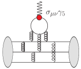
Figure 1: Calculating nEDM requires evaluating the interaction of the em current with the neutron. The contribution of connected and disconnected diagrams from the (left) qEDM and (right) $\Theta$-term.

Contributions from the CEDM and the next order in quark EDM arise due to the change in the action, ${\cal L}_{\rm QCD}\longrightarrow{\cal L}_{\rm QCD}^{\cancel{\text{CP}}}$. In an ideal world, the best way to calculate these effects would be to simulate the lattice theory using a discretized version of ${\cal L}_{\rm QCD}^{\cancel{\text{CP}}}$ and compute the matrix element $\left.\langle N\mid J^{\rm EM}_{\mu}\mid N\rangle\right|_{\cancel{\text{CP}}}$. This ideal approach is not practical because $\cancel{\text{CP}}$ interactions are complex and lattice simulations of theories with a complex action are not yet realistic.

The method of choice is to treat these $\cancel{\text{CP}}$ interactions as perturbations in the small couplings $d_{q}^{\gamma}$ and $d_{q}^{G}$, and expand the theory about ${\cal L}_{\rm QCD}$ (see Sec. 3). Then, the leading terms that contribute to the nEDM are the matrix elements of the product of the electromagnetic current $J^{\rm EM}_{\mu}$ and the 4-volume integral of the operators. For the CEDM operator, the matrix elements that have to be calculated are

$$\left.\langle N\mid J^{\rm EM}_{\mu}\mid N\rangle\right|_{\cancel{\text{CP}}}^{\rm CEDM} = \left\langle N\left|J^{\rm EM}_{\mu}\int d^{4}x[\left(d_{u}^{G}\bar{u}\Sigma_{\nu\kappa}u+d_{d}^{G}\bar{d}\Sigma_{\nu\kappa}d+d_{s}^{G}\bar{s}\Sigma_{\nu\kappa}s+\ldots\right)\tilde{G}^{\nu\kappa}]\right|N\right\rangle\,,$$ (4)

as discussed in Sec. 3. Similarly for the next order qEDM

$$\left.\langle N\mid J^{\rm EM}_{\mu}\mid N\rangle\right|_{\cancel{\text{CP}}}^{\rm qEDM,2} = \left\langle N\left|J^{\rm EM}_{\mu}\int d^{4}x[\left(d_{u}^{F}\bar{u}\Sigma_{\nu\kappa}u+d_{d}^{F}\bar{d}\Sigma_{\nu\kappa}d+d_{s}^{F}\bar{s}\Sigma_{\nu\kappa}s+\ldots\right)\tilde{F}^{\nu\kappa}]\right|N\right\rangle\,.$$ (5)

This second qEDM term has two electromagnetic interactions and is therefore expected to be smaller than the leading term given in Eq. (3). For this reason we neglect its contribution. Finally, the contribution of the $\Theta$-term requires calculating the matrix element:

$$\left.\langle N\mid J^{\rm EM}_{\mu}\mid N\rangle\right|_{\not{\rm CP}}^{\Theta}=\left\langle\left|J^{\rm EM}_{\mu}\ \int d^{4}x\ \Theta G^{\mu\nu}\tilde{G}^{\mu\nu}\right|n\right\rangle\,.$$ (6)

This correlation of $J_{\mu}$ with topological charge $\cal Q$ gives rise to the 2 diagrams shown in Fig. 1 (right).

3 Simulating QCD Including Complex $\cancel{\text{CP}}$ CEDM and $\gamma_{5}$ operators

$$\vbox{\hbox{\includegraphics[width=43.36464pt]{FIGS/qEDM} }}\left(\;\vbox{\hbox{\includegraphics[width=164.77771pt]{FIGS/cEDM_3pt_disc}}}+\vbox{\hbox{\includegraphics[width=164.77771pt]{FIGS/cEDM_3pt}}}\;\right)$$

Figure 2: CEDM contribution is the reweighting factor times the sum of connected and disconnected diagrams.

The QCD Lagrangian becomes complex with the addition of any CP violating interaction. A robust cost-effective method for simulating theories with complex actions does not exist. To calculate the contribution of the $\cancel{\text{CP}}$ interactions to the nEDM, we work within the framework of the Schwinger source method. We start by noting that the fermion part of the Lagrangian, ${\cal L}_{\rm QCD}^{\cancel{\text{CP}}}$ in Eq. (1), involves only quark bilinear operators in presence of the qEDM and CEDM interactions. The fermion fields in the path integral can, therefore, still be integrated out. There are, however, two modifications to the standard calculations of 3-point functions due to the presence of $\cancel{\text{CP}}$ interactions treated as sources. First, the Dirac operator, in the presence of say the CEDM term, becomes

$$\left.\not{D}+m-\frac{r}{2}D^{2}+c_{sw}\Sigma^{\mu\nu}G_{\mu\nu}\right.\mathbin{{\longrightarrow}}\left.\not{D}+m-\frac{r}{2}D^{2}+\Sigma^{\mu\nu}(c_{sw}G_{\mu\nu}+i\epsilon{\tilde{G}_{\mu\nu}})\right.\,.$$ (7)

Quark propagators calculated with this modified Dirac operator include the insertion of the CEDM operator at all space-time points. Second, the Boltzmann weight of all gauge configurations generated without the CEDM term in the action need to be modified by reweighting them by the ratio of the determinants of the Dirac operators for the two theories–with and without $\cancel{\text{CP}}$ terms:

$$\frac{\det(\not{D}+m-\frac{r}{2}D^{2}+\Sigma^{\mu\nu}(c_{sw}G_{\mu\nu}+i\epsilon{\tilde{G}_{\mu\nu}})}{\det(\not{D}+m-\frac{r}{2}D^{2}+c_{sw}\Sigma^{\mu\nu}G_{\mu\nu})}$$ (8)

$$= \exp\mathop{\rm Tr}\nolimits\ln\left[1+i\epsilon\,{\Sigma^{\mu\nu}\tilde{G}_{\mu\nu}}(\not{D}+m-\frac{r}{2}D^{2}+c_{sw}\Sigma^{\mu\nu}G_{\mu\nu})^{-1}\right]$$

$$\approx \exp\left[i\epsilon\mathop{\rm Tr}\nolimits{\Sigma^{\mu\nu}\tilde{G}_{\mu\nu}}(\not{D}+m-\frac{r}{2}D^{2}+c_{sw}\Sigma^{\mu\nu}G_{\mu\nu})^{-1}\right]\,.$$ (9)

Since the coupling $\epsilon$ for the CEDM term for all quark flavors is small, we expect the leading order reweighting factor to be a good approximation. This ‘reweighting factor’ for each gauge configuration is, to leading order, the integral over all spacetime points of the value of a closed quark loop with the insertion of the CEDM operator.

There is an additional challenge: The CEDM operator has an UV divergent mixing with the “$\gamma_{5}$-operator, $\overline{q}\gamma_{5}q/a^{2}$ Bhattacharya:2015rsa . Thus, one has to (i) calculate the matrix element of the “$\gamma_{5}$-operator”, which we do in the same way as for the CEDM operator, (ii) calculate a similar reweighting factor, and (iii) handle the $1/a^{2}$ divergent mixing. Since the reweighting is an overall phase, and configuration to configuration fluctuations can be large, it is therefore important to demonstrate the quality of the signal in $F_{3}(0)$ after reweighting for both the CEDM and $\gamma_{5}$ terms. In Sec. 5, we describe the progress we have made towards addressing these challenges. There is also a mixing of the CEDM operator with the $G^{\mu\nu}\tilde{G}^{\mu\nu}$ operator. Addressing this mixing is part of the calculation of the $\Theta-$term per Eq. (6) Bhattacharya:2015rsa .

The Schwinger source method has allowed us to recast the challenging calculation of 4-point functions given in Eq. (4) to the difficult calculation of 3-point functions Bhattacharya:2016oqm . The Feynman diagrams needed to calculate $\langle N|J_{\mu}^{\rm EM}(q)|N\rangle$ in the presence of CEDM and $\gamma_{5}$ interactions are illustrated in Fig. 2. Starting with an ensemble of gauge configurations generated with a standard lattice action, for example the Wilson-clover action, the steps in the calculation are:

• Calculate propagators, labeled $P$ in Fig. 2, using the standard Wilson-clover Dirac operator. We assume isospin symmetry so the propagators for $u$ and $d$ quarks are numerically the same.

• Calculate a second set of propagators with the CEDM term included with coefficient $\epsilon$ in the Wilson-clover matrix:

  $$\left(\not{D}+m-\frac{r}{2}D^{2}+c_{sw}\Sigma^{\mu\nu}G_{\mu\nu}\right)^{-1}\mathbin{{\longrightarrow}}\left(\not{D}+m-\frac{r}{2}D^{2}+\Sigma^{\mu\nu}(c_{sw}G_{\mu\nu}+i\epsilon{\tilde{G}_{\mu\nu}})\right)^{-1}\,.$$ (10)

  These propagators, labeled $P_{\epsilon}$, include the full effect of inserting the CEDM operator at all possible points along them. The cost of inversion increases by about $7\%$ with respect to $P$, however, using $P$ as the starting guess in the inversion for $P_{\epsilon}$ reduces the number of iterations required by 20–40% depending on the quark mass. The overall average cost of $P_{\epsilon}$ is found to be about 80% of $P$.

• Using $P$ and $P_{\epsilon}$, construct 4 kinds of sequential sources, labeled $P_{u}^{\rm seq}$, $P_{d}^{\rm seq}$, $P_{-\epsilon,u}^{\rm seq}$, and $P_{-\epsilon,d}^{\rm seq}$, at the sink time-slice corresponding to the insertion of a neutron at zero momentum. The subscripts $u$ or $d$ in $P_{u}^{\rm seq}$ and $P_{d}^{\rm seq}$, and similarly in $P_{-\epsilon,u}^{\rm seq}$ and $P_{-\epsilon,d}^{\rm seq}$, denote the flavor of the uncontracted spinor in the neutron source. The minus sign in the coupling, $-\epsilon$, accounts for the backward moving propagator.

• If using the coherent sequential source method, then $N$ sources at different time-slices for the $N$ different calculations being done simultaneously on that configuration, are added together. Sequential propagators with these (coherent) sequential sources are calculated by inverting the Dirac operator with and without the CEDM term as appropriate. The 4 types of (coherent) sequential propagators are shown by the block of 4 correlation functions in the right half of Fig. 2.

• Using the two original and the four sequential propagators, calculate the connected 3-point function. These contractions give the four 3-point functions shown on the right in Fig. 2. Note that a separate insertion of $J_{\mu}^{\rm EM}$ is done on the $u$ and $d$ quark lines.

• Calculate the disconnected quark loop with the insertion of electromagnetic current at zero momentum for each of the quark flavors, $u,\ d,\,s,\ c$ (and $b$ if needed) using the Dirac propagator with and without the CEDM term.

• Calculate the correlation of these quark loops with the appropriate nucleon 2-point correlation functions. The 4 types of disconnected Feynman diagrams required are illustrated in the left of Fig. 2.

• To correct for the omission of the chromo EDM operator in the action during the generation of the gauge configurations, calculate the volume integral of the quark loop with the CEDM insertion for each flavor. Multiply the sum of the connected and disconnected contributions by the reweighting factor–exponential of the estimate of the “CEDM loop” for the configuration with the appropriate coupling factor $i\epsilon$. This is shown by the overall factor in Fig. 2.

• Repeat the calculation for different values of $\epsilon$ that bracket the expected numerical values of the couplings $d_{q}^{G}$ for the various quark flavors.

• Repeat the whole calculation for the $\gamma_{5}$-operator instead of the CEDM operator.

4 Matrix Elements and Form Factors from 3-point Functions

The matrix elements, defined in Eqs. (3), (4) and (6), are extracted from the vacuum to vacuum 3-point correlation function: insertion of the electromagnetic current at times $t$ between the neutron source and sink operators at time $0$ and $T$:

$$\langle\Omega|{N(\vec{0},0)J^{\rm EM}_{\mu}(\vec{q},t)N^{\dagger}(\vec{p},T)}|\Omega\rangle=\sum_{N,N^{\prime}}u_{N}e^{-M_{N}t}\;{\langle N|J^{\rm EM}_{\mu}(q)|N^{\prime}\rangle}\;e^{-E_{N^{\prime}}(T-t)}{\overline{u}}_{N}^{\prime}\,.$$ (11)

where in the right hand side we have used the expansion in a complete basis of states $|N\rangle,|N^{\prime}\rangle,\ldots$ that couple to the neutron interpolating operator $N$. We use $N\equiv\epsilon^{abc}[{d}^{a{\rm T}}C\gamma_{5}(1+\gamma_{4})u^{b}]d^{c}$ where $C=\gamma_{0}\gamma_{2}$ is the charge conjugation matrix, $a,\ b,c$ are the color indices, $u,\ d$ are the quark flavors, $u_{N}$ is the free neutron spinor and $M_{N}$ is the neutron mass. In the presence of $\cancel{\text{CP}}$, the nucleon 2-point function is

$$\langle\Omega|{N(\vec{0},0)N^{\dagger}(\vec{p},t)}|\Omega\rangle|_{\lim{t\to\infty}}=A^{2}u_{N}\,e^{-p_{4}t}\,{\overline{u}}_{N}=A^{2}e^{-p_{4}t}{e^{i\alpha_{N}\gamma_{5}}}(i\not{p}+m_{N}){e^{i\alpha_{N}\gamma_{5}}}\,,$$ (12)

where the phase angle $\alpha_{N}$ arises due to the $\cancel{\text{CP}}$ coupling $\epsilon$ and depends on it. To determine the desired region of linearity of $\alpha$ versus $\epsilon$ we show the imaginary part of the neutron 2-point function in Fig. 3. It demonstrates the quality of the signal for $\alpha$ for appropriately small values of $\epsilon$ on two different ensembles. Fig. 4 shows the expected linear behavior of $\alpha$ versus $\epsilon$ over a range of small $\epsilon$.

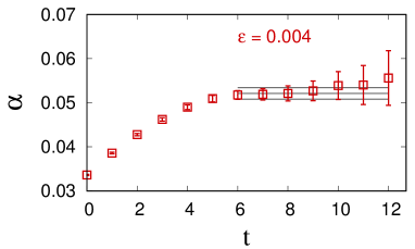
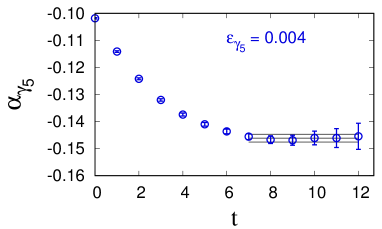
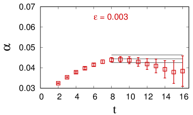
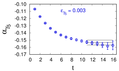
Figure 3: The phase $\alpha$ extracted from the plateau in the imaginary part of the neutron 2-point function with $\epsilon=0.004$ on the $a12m310$ ensemble (top) and $\epsilon=0.003$ on the $a09m310$ ensemble (bottom). The plots on the left are for the CEDM operator and on the right for the $\gamma_{5}$ mixing operator.

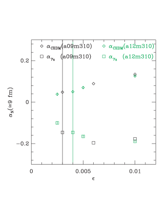
Figure 4: Linear behavior of the phase $\alpha$ versus $\epsilon$ with the insertion of the CEDM and the $\gamma_{5}$ operators.

Once the matrix element of the electromagnetic current, $J^{\rm EM}_{\mu}(q)$ defined in Eq. 2, within the nucleon state is extracted using Eq. (11), it is parameterized in terms of four Lorentz covariant form factors $F_{1}$, $F_{2}$, $F_{A}$ and $F_{3}$:

$$\langle N|J_{\mu}^{\rm EM}(q)|N\rangle = \overline{u}_{N}\left[\gamma_{\mu}\;F_{1}(q^{2})\quad+\quad i\sigma^{\mu\nu}\;q_{\nu}\;\frac{F_{2}(q^{2})}{2M_{N}}\right.$$ (13)

$$\left.+\quad{(2i\,M_{N}\gamma_{5}q_{\mu}-\gamma_{\mu}\gamma_{5}q^{2})\;\frac{F_{A}(q^{2})}{M_{N}^{2}}}\quad+\quad\sigma^{\mu\nu}\;q_{\nu}\gamma_{5}\;\frac{F_{3}(q^{2})}{2M_{N}}\right]u_{N}\,,$$

$F_{1}$ and $F_{2}$ are the standard Dirac and Pauli form factors. The anapole form factor $F_{A}$ violates parity P and the electric dipole form factor $F_{3}$ violates P and CP. $F_{3}$ is extracted from the different matrix elements by using different combinations of the momentum transfer $q_{\mu}$ and spin projections. The zero momentum limit of these form factors gives the charges and dipole moments: the electric charge is $F_{1}(0)=1$ and the anomalous magnetic dipole moment is $F_{2}(0)/2M_{N}$. The contribution of the matrix element of each $\cancel{\text{CP}}$ interaction defined in Eqs. (3), (4), and (6) to the electric dipole moment of the neutron is given by $d_{n}=\lim_{q^{2}\to 0}{F_{3}(q^{2})}/{2M_{n}}\,.$

5 Status of Numerical Calculations

So far, we have performed numerical calculations on two 2+1+1-flavor HISQ ensembles generated by the MILC collaboration Bazavov:2012xda . The first, labeled $a12m310$, has $a=0.12$ fm and $M_{\pi}=310$ MeV and the second, labeled $a09m310$, has $a=0.09$ fm and $M_{\pi}=310$ MeV. The correlation functions are constructed using Wilson-clover fermions. On the $a12m310$ ($a09m310$) ensemble we have analyzed 400 (270) configurations with 64 measurements on each configuration. The ensembles used and our strategy for the calculation of 2- and 3-point functions with this clover-on-HISQ approach are described in Ref. Bhattacharya:2016zcn .

In Fig. 5, we show the data for $F_{3}$ from the connected diagrams in the presence of the CEDM term, and in Fig. 6, the data for $F_{3}$ in the presence of the $\gamma_{5}$ term. The data are presented for three values of the source-sink separation $\mathop{t_{\rm sep}}\nolimits=8,10$ and $12$. The excited-state contamination in the matrix elements, and thus in $F_{3}$, is removed by taking the $\mathop{t_{\rm sep}\to\infty}\nolimits$ limit. These figures show that an acceptable signal-to-noise ratio can be obtained to estimate $F_{3}$ with $O(1)$ errors, our first goal for the CEDM calculations.

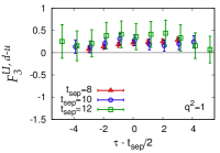
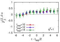
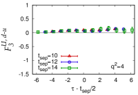
Figure 5: Illustration of the signal in $F_{3}$ with the inclusion of the CEDM term. The data in the top row are for $\vec{p}=(1,0,0)\times 2\pi/La$ in the following order: insertion on $u$ and $d$ quarks for the $a12m310$ ensemble followed by insertion on $u$ and $d$ quarks for the $a09m310$ ensemble. The plots in the second row are in the same order except with $\vec{p}=(2,0,0)\times 2\pi/La$.

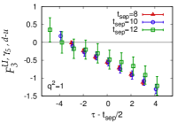
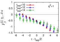
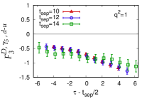
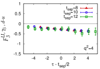
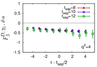
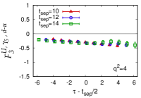
Figure 6: Illustration of the signal in $F_{3}$ with the inclusion of the $\gamma_{5}$ term. The data in the top row are for $\vec{p}=(1,0,0)\times 2\pi/La$ in the following order: insertion on $u$ and $d$ quarks for the $a12m310$ ensemble followed by insertion on $u$ and $d$ quarks for the $a09m310$ ensemble. The plots in the second row are in the same order except with $\vec{p}=(2,0,0)$.

There are theoretical reasons to expect that the connected contribution of the $\gamma_{5}$ operator is, with small corrections, proportional to that of the CEDM operator Bhattacharya:2016lat . In Fig. 7, we show the ratio of the two contributions and find that this expectation is actually realized.

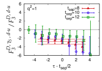
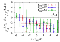
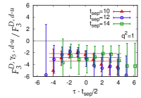
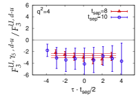
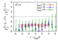
Figure 7: The ratio of the connected contribution of the $\gamma_{5}$ term to the CEDM term in the $F_{3}$ form factor. The rest is the same as in Fig. 5.

To conclude, the data so far show that an acceptable signal-to-noise ratio can be obtained in the connected contributions to $F_{3}$ for both the CEDM and $\gamma_{5}$ operator insertion. We also find that The ratio of the connected contribution of the $\gamma_{5}$ to CEDM term is a constant. This implies that the mixing of the $\gamma_{5}$ term with the CEDM term can be cast as part of the multiplicative renormalization of the CEDM operator. Controlling its $O(1/a^{2})$ UV divergent coefficient is a hurdle for lattice theories that respect chiral symmetry (domain wall or overlap fermions) and those that don’t such as Wilson-clover fermions. Work to address the full mixing of the CEDM operator and the calculation of the disconnected diagrams and the reweighting factors is under progress.

References

- (1) C. Bennett et al., Astrophys.J.Suppl. 148, 1-27 (2003).
- (2) E. W. Kolb and M. S. Turner, Front. Phys. 69, 1-547 (1990).
- (3) P. Coppi, eConf C040802, L017 (2004).
- (4) A.D. Sakharov, Pisma Zh. Eksp. Teor. Fiz. 5 32â35 ( 1967).
- (5) M. Kobayashi and T. Maskawa, Prog.Theor.Phys. 49 652-657 (1973).
- (6) H. Nunokawa, et al., Prog.Part.Nucl.Phys. 60, 338-402 (2008).
- (7) A. D. Dolgov, Phys. Rept. 222, 309â386 (1992).
- (8) T. Bhattacharya, et al., Phys. Rev. D92, 094511 (2015).
- (9) T. Bhattacharya, et al., Phys. Rev. Lett, 115 212002 (2015).
- (10) T. Bhattacharya, et al., Phys. Rev. D92, 114026 (2015).
- (11) T. Bhattacharya, et al., PoS LATTICE2015, 238 (2016).
- (12) T. Bhattacharya, et al., Phys. Rev. D94, 054508 (2016).
- (13) T. Bhattacharya, et al., PoS LATTICE2016, 001 (2016).
- (14) A. Bazavov, et al., Phys. Rev. D92, 114026 (2015).
- (15) R. G. Edwards and B. Joo, Nucl. Phys. Proc. Suppl. 140 832-837 (2005).