Quasi-stationary states in nonlocal stochastic growth models with infinitely many absorbing states

Abstract

We study a two parameter ($u,p$) extension of the conformally invariant raise and peel model. The model also represents a nonlocal and biased-asymmetric exclusion process with local and nonlocal jumps of excluded volume particles in the lattice. The model exhibits an unusual and interesting critical phase where, in the bulk limit, there are an infinite number of absorbing states. In spite of these absorbing states the system stays, during a time that increases exponentially with the lattice size, in a critical quasi-stationary state. In this critical phase the critical exponents depend only on one of the parameters defining the model ($u$). The endpoint of this critical phase, where the system changes from an active to an inactive frozen phase, belongs to a distinct universality class. This new behavior, we believe, is due to the appearance of Jordan cells in the Hamiltonian describing the time evolution. The dimensions of these cells increase with the lattice size. In a special case ($u=0$) where the model has no adsorptions we are able to calculate analytically the time evolution of some observables. A polynomial time dependence is obtained thanks to the appearance of Jordan cells structures in the Hamiltonian.

1 Introduction

Stochastic growth models of interfaces have been extensively studied along the years (see [1, 2, 3] for reviews). The most studied universality class of critical dynamics behavior of growing interfaces are the ones represented by the Edward-Wilkinson (EW) [4] and the Kardar-Parisi-Zhang (KPZ) [5] models whose dynamical critical exponents are equal to 2 and $3/2$, respectively. Differently from these models, where the absorption and desorption processes are local, the raise and peel model (RPM) [6], although keeping the adsorption process local, the desorption processes is nonlocal. This model is quite interesting, as it is the first example of an stochastic model with conformal invariance. The critical properties of the model depend on the parameter $u$ defined as the ratio among the adsorption and desorption rates. At $u=1$ the RPM is special, being exact integrable and conformally invariant. The dynamical critical exponent has the value $z=1$ and its time-evolution operator (Hamiltonian) is related to the XXZ quantum chain with $z$-anisotropy $\Delta=-\frac{1}{2}$ (Razumov-Stroganov point [7]). For $u<1$ (desorption rates greater than the adsorption ones) the model is noncritical, but for $u\geq 1$ the model is in a critical regime with continuously varying critical exponents $z=z(u)$, that decreases from $z(1)=1$ (conformally invariant) to $z(u\to\infty)=0$.

The configurations of the growing surface in the RPM are formed by sites whose heights define Dyck paths on a lattice with $L+1$ sites ($L$ even) and open boundaries. These are staircase walks with integer horizontal steps that go from $(x,y)=(0,0)$ to $(L/2,L/2)$ and are never lower than the ground $x=0$ or higher than the diagonal $x=y$[8]. In these surface configurations there are active sites where adsorption and desorption processes take place, and inactive sites where nothing happens during the time evolution.

An interesting extension of the RPM at $u=1$, proposed in [9], is the peak adjusted raise and peel model (PARPM). In this model an additional parameter $p$ that depends on the total number of inactive sites, controls the relative changes of a given configuration. The model at $p=1$ recovers the RPM. For $p\neq 1$ the model is not exact integrable anymore but still is conformally invariant [9]. The parameter $p$ in the PARPM has a limiting value ($p={p}_{1}=2$) where the configuration with only inactive sites (no adsorption or desorption) become an absorbing state. Surprisingly at this point, on spite of the presence of the absorbing state, that should be the true stationary state, the system stays in a quasi-stationary state during a time interval that grows exponentially with the system size [12]. This quasi-stationary state has similar properties as the stationary states of the conformally invariant region $p<{p}_{1}$.

Motivated by this unusual and interesting behavior we introduce in this paper an extension of the PARPM, where the parameter $p$ is extended so that when $p>{p}_{1}$ the number of absorbing states increases with the value of $p$. The results presented in this paper shows that a quasi-stationary state, with similar properties as in the conformally invariant region $p<{p}_{1}$, endures as the true stationary state even when the number of absorbing states is extensively large. Only at $p=p_{c}>{p}_{1}$ the model undergoes a transition to one of the infinitely many absorbing states.

In order to check if this unusual behavior is linked to the conformal invariance of the model for $p<{p}_{1}$ we study the PARPM in regions where $u\neq 1$, where the model is either gaped ($u<1$), or critical but not conformally invariant ($u>1$). An overview of our results is given in the schematic phase diagram of the model shown in Fig. 1.

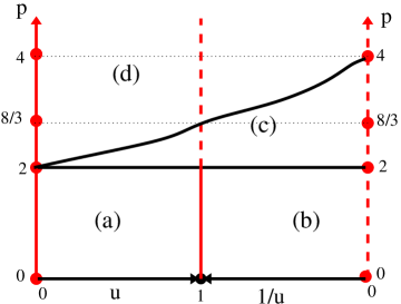
Figure 1: Schematic phase diagram of the PARPM in terms of the parameters $p$ and $u$ (or $1/u$). The phases are: (a) non critical with no absorbing states; (b) critical with no absorbing states; (c) critical with infinitely many absorbing states (active); (d) inactive phase where the system is frozen in one of the infinitely many absorbing states. Line $u=0$ ($0\leq p<2$): the model has a gap (massive) but with a behavior that resembles a critical system (see section 3). Line $u=1$ ($0\leq p<8/3$): the model is critical and conformally invariant (see section 4). Line $1/u=0$ ($0\leq p<4$): the model is related to an extended TASEP model with non-local jumps of particles (see section 5). The straight line $p=2$ ($0<u<\infty$) separates the phases (a) and (b), having no absorbing states, from the phase (c) with infinitely many absorbing states. The black line connecting $(u,p)=(0,2)$ to $(u,p)=(0,4)$ is a critical line separating the phase (c) with infinitely many absorbing states from the frozen phase (d).

In this paper we are going to restrict ourselves to the representative cases (red lines in Fig. 1), where $u=1$, $u=0$ (no adsorption) and $u=\infty$ (no desorption), with arbitrary values of $p$.

The RPM although originally defined in an open chain can also be defined in a periodic lattice [13]. In the periodic chain the model can be interpreted as a particular extension of the asymmetric exclusion process (ASEP) where the particles (excluded volume) are allowed to perform local as well nonlocal jumps. We are going also to consider in this paper the PARPM formulated in periodic lattices. We verified that when $u\to\infty$ (only adsorption processes) the extended PARPM is exactly related to a totally asymmetric exclusion process (TASEP) where the particles jumps only in one direction. At $p=1$, where the model recovers the RPM, the model is mapped to the standard TASEP [14, 15], and for $p\neq 1$ it can be interpreted as a TASEP whose transition rate to the neighboring sites depend on the total number of particle-vacancy pairs, in the configuration.

At $u=0$ (no adsorption) the model is gapped but shows interesting properties. The configuration where there are no sites available for desorption is an absorbing state, since there is not adsorption process. Although gapped the system stays during a large time, that increases polynomially with the lattice size, in a critical quasi-stationary state with dynamical critical exponent $z=1$. This phenomena is due to the appearance of an extensively large number of Jordan cells (or Jordan blocks), that for sufficiently large lattices produces a more important effect than the exponential decay induced by the gap. For some special initial conditions we are able to obtain analytically the Jordan cells and derive the time dependence of some of the observables. Actually Jordan cells are known to appear in models described by Temperley-Lieb algebra (TLA) and whose continuum limit are ruled by logarithmic conformal field theories [16, 17]. Although the time evolution operator of the RPM is given by the sum of generators of the (TLA), the introduction of the parameter $p$, producing the PARPM, destroys this connection due to the appearance of nonlocal terms that are not expressed in a simple way in terms of the generators of the TLA.

The paper is organized as follows. In the next section we introduce the extension of the PARPM studied in this paper, for open and periodic boundary conditions. We present our results separately in sections 3, 4 and 5 for the model with $u=0$, $u=1$ and $u\to\infty$, respectively. Finally in section 6 we present our conclusions.

2 The peak adjusted raise and peel model

The raise and peel model (RPM) and the peak adjusted model (PARPM) are models describing the stochastic time evolution of an interface defined by a set of integer heights in a discrete lattice of size $L$ (even). These heights are $\{h_{0},h_{1},\ldots,h_{L}\}$ and $\{h_{1},h_{2},\ldots,h_{L}\}$ for the case of open and periodic boundary conditions, respectively. The height configurations satisfy the restricted solid-on-solid conditions

$$|h_{i+1}-h_{i}|=1,\quad h_{i}\in Z.$$ (2.1)

The boundary condition imposes the additional constraints: (a) for the periodic case $h_{i}=h_{L+1}$ ($h_{i}\in Z$) and the configurations $\{h_{i}\}$ and $\{h_{i}+m\}$ ($m\in Z$)are the same, (b) for the open case $h_{0}=h_{L}=0$ and $h_{i}$ are non-negative integers ($h_{i}\geq 0$). The number of profile configurations of the surface is [13, 6]:

$$Z_{b}(L)=\frac{L!}{(\frac{L}{2})!(\frac{L}{2}+b)!},$$ (2.2)

where $b=0$ and $b=1$ for the periodic and open cases, respectively.

The configurations have a local minimum (valley) or a local maximum (peak) whenever $h_{i-1}>h_{i}<h_{i+1}$ or $h_{i-1}<h_{i}>h_{i+1}$, respectively. We call for convenience, the configuration with the maximum number of peaks $N_{p}=L/2$ as the substrate, and the configuration with the minimum number of peaks $N_{p}=1$ as pyramid. In Fig. 2 we show examples of these configurations for the case where the lattice has $L=6$ sites and open boundary conditions.

Figure 2: Special configuration of the PARPM with $L=6$ sites and open boundary conditions. a) The pyramid configuration. b) The substrate configuration.

In the dynamics of the RPM each site in a unit of time is visited with equal probability. The PARPM however has the additional parameter $p$ that has the net effect of increasing ($p>1$) or decreasing ($p<1$) the visiting probability for the sites with local peaks. For a given configuration the parameter $p\geq 0$ fix the probability that a particular peak is visited as $p_{p}=\frac{1}{L-b}p$, where $b=0,1$ for periodic and open ends. If a given configuration contains $N_{p}$ peaks, the probability $P_{p}$ that an arbitrary peak is visited is [9]

$$P_{p}=N_{p}p_{p}=\frac{N_{p}p}{L-b},$$ (2.3)

while the probability that the remaining $N_{np}=L-b-N_{p}$ sites (sites with no peaks) are visited is given by

$$P_{np}=1-P_{p}=\frac{L-b-N_{p}p}{L-b}=q\frac{N_{np}}{L-b},$$ (2.4)

where the parameter $q$ gives the probability that a particular site, which is not a peak, is visited. This is not a new parameter, it depends on the parameter $p$ and the number $N_{p}$ of peaks in the configuration:

$$q=\frac{L-b-N_{p}p}{L-b-N_{p}}.$$ (2.5)

Since the maximum number of peaks is $\frac{L}{2}$, $p$ should be restricted to the values:

$$0\leq p\leq{p}_{1},\mbox{ where }{p}_{1}=2\frac{L-b}{L},\quad(b=0,1).$$ (2.6)

For $p=1$ all the sites are visited with equal probability independently of being peaks or not and we recover the standard RPM. For values of $p>1$ ($p<1$) the peaks have a larger (smaller) chance to be visited in a time interval. At $p=0$ no peaks are visited in a unit of time. At $p={p}_{1}$ the visited sites in the configuration with $\frac{L}{2}$ peaks (substrate) are only the ones with peaks.

In this paper we generalize the definition of $p$ given in (2.3), producing a richer model as we shall see. Given a configuration with $N_{p}$ peaks we now extend (2.3) by imposing that in a unit of time the peaks are visited with probability

$$P_{p}=\mbox{Min}\left\{1,\frac{N_{p}}{L-b}p\right\},\quad b=0,1,$$ (2.7)

where, as before $b=0$ ($b=1$) for periodic (open) boundary conditions. The probability $q$ that a particular site that is not a peak is visited is given, using (2.7) and (2.4), by

$$q=\mbox{Max}\left\{\frac{L-b-N_{p}p}{L-b-N_{p}},0\right\}.$$ (2.8)

Now the parameter $p$ can be any non-negative number. For $p\geq{p_{1}}=2(L-b)/L$ all the configurations with number of peaks $N_{p}\geq\frac{L-b}{p}$ will be visited only at the sites containing peaks.

We now define the dynamical rules for the stochastic evolution of the PARPM model. We can imagine a height configuration as a surface separating a solid phase from a gaseous one formed by tilted blocks that hit the surface. In a unit of time the blocks hit the sites with peaks ($h_{i-1}<h_{i}>h_{i+1}$), valleys ($h_{i-1}>h_{i}<h_{i+1}$), positive slope ($h_{i-1}<h_{i}<h_{i+1}$) or negative slope ($h_{i-1}>h_{i}>h_{i+1}$). The probability $P_{p}$ that we hit the sites that have a peak is given by (2.7), while the probability that we reach the other non-peak sites is $P_{np}=1-P_{p}$. In a unit of time the following processes may occur (see Fig. 3), after a tile hits a site $i$:

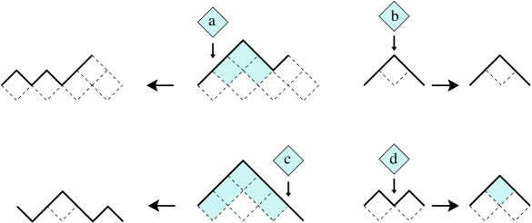
Figure 3: The dynamical processes in the PARPM. The tilted tile in the gaseous phase hit a positive slope (a), a peak in (b), a negative slope in (c) and a valley in (d) (see the text).

a) If we have a peak ($h_{i-1}<h_{i}>h_{i+1}$) the tile is reflected and the surface is unchanged (see Fig. 3b).

b) If we have a valley ($h_{i-1}>h_{i}<h_{i+1}$), with probability proportional to the adsorption rate $u_{a}$, the configuration is changed $h_{i}\to h_{i}+2$ by adsorbing the tile (see Fig. 3d).

c) If we have a positive slope ($h_{i-1}<h_{i}<h_{i+1}$), with a probability proportional to the desorption rate $u_{d}$, the tilted tile is reflected after desorbing ($h_{j}\to h_{j}-2$) a layer of $t-1$ tiles from the sites $\{j=i+1,\ldots,i+t-1\}$, where $h_{j}>h_{i}=h_{i+t}$ (see Fig. 3a), i.e. $t$ is the minimum number of added sites to the right where the original height is repeated $h_{i}=h_{i+t}$.

d) If we have a negative slope ($h_{i-1}>h_{i}>h_{i+1}$), with a probability proportional to the desorption rate $u_{d}$, the tilted tile is reflected after desorbing ($h_{j}\to h_{j}-2$) a layer of $t-1$ tiles from the sites $\{j=i-t+1,\ldots,i-1\}$, where $h_{j}>h_{i}=h_{i-t}$ (see Fig. 3c), i.e. $t$ is the minimum number of subtracted sites to the left where the original height is repeated $h_{i}=h_{i-t}$.

In a continuous time evolution, the probability $P_{c}(t)$ of finding the system in the configuration $c=1,2,\ldots,Z_{b}(L)$ in a given time is given by the master equation:

$$\frac{dP_{c}(t)}{dt}=-\sum_{c^{\prime}}H_{c,c^{\prime}}P_{c^{\prime}}(t),$$ (2.9)

that can be interpreted as an Schrödinger equation in imaginary time. The above defined stochastic rules give us the matrix elements $H_{c,c^{\prime}}$ of the $Z_{b}(L)$-dimensional Hamiltonian. The Hamiltonian is an intensity matrix, i.e., the non-diagonal elements are negative and $\sum_{c}H_{c,c^{\prime}}=0$. This imply that the ground state of the system $|0\rangle$ has eigenvalue 0 and its components give us the probabilities $P_{c}$ of the configurations in the stationary state, i.e.,

$$|0\rangle=\sum_{c}P_{c}|c\rangle,\quad P_{c}=\lim_{t\to\infty}P_{c}(t).$$

The matrix elements $H_{c,c^{\prime}}$ are calculated as follows. Only configurations that are connected through adsorption and desorption processes give non-zero values. This means that apart from a multiplicative constant, that can be absorbed in the time scale, the matrix elements of the Hamiltonian is only a function of the ratio $u=\frac{u_{a}}{u_{d}}$. A configuration $|c\rangle$ with $N_{p}(c)$ peaks have $L-b-N_{p}(c)=N_{np}(c)$ sites where the desorption or adsorption processes may occur. Each of these $N_{np}(c)$ sites are reached with probability $q(c)$ defined in (2.8). The non-diagonal elements $H_{c,c^{\prime}}$ are given by $-u_{a}q(c^{\prime})$, $-u_{d}q(c^{\prime})$, or $-2u_{d}q(c^{\prime})$, if the configuration $|c\rangle$ and $|c^{\prime}\rangle$ are connected by a single adsorption, one, or two distinct desorptions, respectively. The diagonal elements are calculated from the non-diagonal ones since $H_{c,c}=-\sum_{c\neq c^{\prime}}H_{c,c^{\prime}}$.

As an illustration let us consider the case of a lattice size $L=6$ with open ends ($b=1$). In this case there are $Z_{1}(6)=5$ configurations $|c\rangle$ ($c=1,\ldots,5$), that are shown in Fig. 4. The number of peaks in each configuration give us, using (2.8): $q(1)=[(5-p)/4]_{0}$, $q(2)=q(3)=q(4)=[(5-2p)/3]_{0}$ and $q(5)=[(5-3p)/2]_{0}$, where we denote hereafter the maximum value:

$$[x]_{0}=\mbox{Max}\{0,x\}.$$ (2.10)

Figure 4: The five configurations of the PARPM for a lattice with $L=6$ sites and open boundary conditions.

The configuration $|1\rangle$ ($|5\rangle$) with lowest (largest) number of peaks is the one we called pyramid (substrate). The name substrate come from the fact that all the configurations can be obtained from it by the successive additions of tilted tiles. The configuration $|1\rangle$ is connected to $|2\rangle$ by a desorption at site 2 or 4. The configuration $|2\rangle$ is connected to the configuration $|1\rangle$ by an adsorption at site 3 and to the configurations $|4\rangle$ and $|3\rangle$ by a desorption at site 1 and 5, respectively. Following similarly with the other configurations we obtain the $5\times 5$ Hamiltonian:

$$H=-\left(\begin{array}[]{c|rrrrr}&\langle 1|&\langle 2|&\langle 3|&\langle 4|&\langle 5|\\ \hline\cr|1\rangle&[4u_{d}\frac{5-p}{4}]_{0}&-[u_{a}\frac{5-2p}{3}]_{0}&0&0&0\\ |2\rangle&-[2u_{d}\frac{5-p}{4}]_{0}&[(u_{a}+2u_{d})\frac{5-2p}{3}]_{0}&-[u_{a}\frac{5-2p}{3}]_{0}&-[u_{a}\frac{5-2p}{3}]_{0}&0\\ |3\rangle&0&-[u_{d}\frac{5-2p}{3}]_{0}&[(u_{a}+2u_{d})\frac{5-2p}{3}]_{0}&0&-[u_{a}\frac{5-3p}{2}]_{0}\\ |4\rangle&0&-[u_{d}\frac{5-2p}{3}]_{0}&0&[(u_{a}+2u_{d})\frac{5-2p}{3}]_{0}&-[u_{a}\frac{5-3p}{2}]_{0}\\ |5\rangle&-[2u_{d}\frac{5-p}{4}]_{0}&0&-[2u_{d}\frac{5-2p}{3}]_{0}&-[2u_{d}\frac{5-2p}{3}]_{0}&[2u_{a}\frac{5-3p}{2}]_{0}\end{array}\right).$$ (2.17)

We observe that for arbitrary values of $p\geq 0$, when the adsorption (desorption) is absent $u_{a}=0$ ($u_{d}=0$) the matrix elements connecting the configuration $|5\rangle$ ($|1\rangle$) that we called substrate (pyramid) are zero. The configurations $|1\rangle$ and $|5\rangle$ are in this case absorbing states. This is valid for general lattice sizes. Once the system reaches these configurations it stays on them forever. The Hamiltonian (2.17) for $0\leq p\leq{p}_{1}=5/3$ and $u=1$ recovers the one in the original formulation of the PARPM, introduced in [9]. In the extended version of the model (2.17) we see that for arbitrary values of $u$ we have no absorbing states as long $0\leq p<{p}_{1}=5/3$. At $p={p}_{1}=5/3$ the configuration $|5\rangle$ (substrate) becomes an absorbing state. For ${p}_{1}\leq p<{p}_{2}=5/2$, the configuration $|5\rangle$ is the single absorbing state. For ${p}_{2}\leq p<{p}_{3}=5$, the configurations $|2\rangle$, $|3\rangle$ and $|4\rangle$ containing two peaks also become absorbing states. Finally for $p\geq{p}_{3}$ all the configurations are absorbing states.

The proliferation of absorbing states when $p\geq{p}_{1}$ is one of the main features of the PARPM. For arbitrary values of $u=u_{a}/u_{d}$ and lattice sizes $L$, it is convenient to define

$${p}_{i}=2\frac{L-b}{L+2-2i},\quad i=1,2,\ldots,L/2,$$ (2.19)

where $b=0,1$ for periodic and open boundaries. For ${p}_{i}\leq p<{p}_{i+1}$ all the configurations with $N_{p}\geq\frac{L}{2}-i+1$ are absorbing states. The number of configurations with $N_{p}=\frac{L}{2}-i+1$, grow very fast as $i$ increases and we should expect an interesting behavior once $p>{p}_{1}$.

The model at $u=1$ and for $p<{p}_{1}$ is known to be critical and conformally invariant [9]. At $p=1$, where the model recovers the standard RPM, the model in non-critical (gapped) for $u<1$ and gapless for $u\geq 1$. For an overview of the phase diagram of the model see Fig. 1. In the next sections we are going to study the model for arbitrary values of $p$, but considering only the three representative cases where $u=0$, $u=1$ and $u=\infty$ (red lines in Fig. 1), that we have distinct physical properties. In these sections we are going to measure several observables. The average height at time $t$ is defined as:

$$h_{L}(t)=\frac{1}{L}\sum_{i=1}^{L}<h_{i}(t)>,$$ (2.20)

where $<h_{i}(t)>$ is the average height at the site $i$. In a given configuration, we define as contact points the points where the profile touch the substrate. In the open boundaries case their average are:

$$K_{L}(t)=<\sum_{i=1}^{L-1}\delta_{h_{i}(t),0}>,$$ (2.21)

while for the periodic case:

$$K_{L}(t)=<\sum_{i=1}^{L}\delta_{h_{i}(t)-h_{\scriptsize{\mbox{min}}},0}>,$$ (2.22)

where $h_{\mbox{\scriptsize{min}}}$ is the minimum height in the configuration. Another interesting quantity is the number of peaks and valleys in the configuration. The related observable is:

$$\tau_{L}(t)=\frac{1}{L-b}\sum_{i=1}^{L-b}\left(1-\frac{|h_{i-1}-h_{i+1}|}{2}\right),\quad b=0,1.$$ (2.23)

3 The model with no adsorptions

We consider in this section the limiting case of the PARPM where we have no adsorptions, i. e., $u=u_{a}/u_{d}=0$. In this case by ordering the configurations according to their number or peaks, i. e., the first state is the pyramid ($N_{p}=1$) and the last one the substrate ($N_{p}=L/2$), the Hamiltonian in the master equation (2.9) is a lower triangular matrix. This happens because we have only desorptions and their effect in the configurations is the increase of the number of peaks. An example for $L=6$ with open boundary condition ($b=1$) is obtained by setting $u_{a}=0$ in (2.17). Since $H$ is a lower triangular matrix its $Z_{b}(L)$ eigenvalues are given by its diagonal elements $H_{c,c}$ ($c=1,\ldots,Z_{b}(L)$). The diagonal elements in the PARPM are given by

$$H_{c,c}=(N_{s}^{(c)}u_{d}+N_{v}^{(c)}u_{a})q(c),$$ (3.1)

where $N_{s}^{(c)}$ and $N_{v}^{(c)}$ are the number of sites where we have a nonzero slope and valleys, respectively. The $p$-dependent parameter $q(c)$ is given by (2.8). For the case of no adsorption, we then have the eigenvalues

$$E(N_{p},p,L,u_{d})=\mbox{Max}\left\{0,u_{d}(L-2N_{p})\frac{L-b-N_{p}p}{L-b-N_{p}}\right\},$$ (3.2)

where we have used (2.8) and the fact that $N_{s}=L-2N_{p}$.

The present case, where $u_{a}=0$, the results for the periodic case can be obtained from the open boundary case straightforwardly. We are going, in the rest of this section, to restrict ourselves to the open boundary case where $b=1$. It is convenient to label the energies (3.2) by the index $i=L/2-N_{p}$:

$$E_{i}=\mbox{Max}\left\{0,2iu_{d}\frac{(2-p)L+2(ip-1)}{L+2(i-1)}\right\},\quad i=0,1,\ldots,L/2$$ (3.3)

Let us restrict ourselves initially to the cases where the parameter $p\leq 2$. The stationary state of the system is the substrate, being the ground-state ($E_{0}=0$) of the Hamiltonian. In this no adsorption case the ground state is also an absorbing state. If the initial configuration is not the substrate, for sufficiently large times the dynamics will be ruled by the first gap of the Hamiltonian $E_{1}-E_{0}=E_{1}$, given by (3.3), and since $E_{1}$ is finite for any $L$, we do expect for any observable an exponential time-decay $\tau\sim 1/E_{1}$. However we need some care in this analysis since the eigenvalue $E_{1}$ has a degeneracy $d_{\frac{L}{2}-1}=(\frac{L}{2}-1)(\frac{L}{4})$. This is the number of configurations with $N_{p}=\frac{L}{2}-1$ peaks, obtained by adding tiles in the first layer ($h_{i}\leq 2$) above the substrate and with the tiles in the closest positions (no nonzero slopes between the added tiles) (see Fig. 5 for examples). For large $L$ the degeneracy grows as $L^{2}$ and as we shall see, an interesting physical behavior occurs.

Figure 5: Configurations $|N_{0},k\rangle$ with $(\frac{L}{2}-1)$ peaks obtained by adding, in the substrate configuration, $N_{0}$ tiles at the closest positions. The index $k$ indicate the valley position in the substrate where the initial tile is added. The substrate configuration $|SUBS\rangle$ is also shown.

To simplify our analysis we are going to consider as the initial state, for the evolution of our system, one of the configurations with $L/2-1$ peaks, and with $N_{0}$ tiles added in the substrate. There are $L/2-N_{0}$ configurations of this kind and we denote them as $|N_{0},k\rangle$, $k=1,\ldots,L/2-N_{0}$; $N_{0}=1,\ldots,L/2-1$. As an example, we show in Fig. 5 some of the configurations for a lattice size $L=14$, together with the substrate absorbing state $|\mbox{SUBS}\rangle$.

If we chose for $L=14$ the state $|3,2\rangle$ (see Fig. 5) as the initial state, the effective Hamiltonian is given by

$$H=-\left(\begin{array}[]{c|rrrrrrr}&|3,2\rangle&|2,2\rangle&|2,3\rangle&|1,2\rangle&|1,3\rangle&|1,4\rangle&|\mbox{SUBS}\rangle\\ \hline\cr\langle 3,2|&E_{1}&0&0&0&0&0&0\\ \langle 2,2|&-E_{1}/2&E_{1}&0&0&0&0&0\\ \langle 2,3|&-E_{1}/2&0&E_{1}&0&0&0&0\\ \langle 1,2|&0&-E_{1}/2&0&E_{1}&0&0&0\\ \langle 1,3|&0&-E_{1}/2&-E_{1}/2&0&E_{1}&0&0\\ \langle 1,4|&0&0&-E_{1}/2&0&0&E_{1}&0\\ \langle\mbox{SUBS}|&0&0&0&-E_{1}&-E_{1}&-E_{1}&0\\ \end{array}\right),$$ (3.12)

where $E_{1}$ is given by (3.3). It is interesting to note that $H$ in (3.12) has a Jordan-cell structure, since although the eigenvalue $E_{1}$ is 6 degenerated there are only 3 distinct eigenvectors. In the general case, for arbitrary $L$, if we start with an configuration with $L/2-1$ peaks and $N_{0}$ tiles added in the substrate, we have a Jordan-cell structure where instead of $N_{0}(N_{0}+1)/2$ eigenvectors with eigenvalue $E_{1}$, we have only $N_{0}$ distinct eigenvectors ($N_{0}(N_{0}-1)/2$ are missing!). If we start, for large $L$, with an initial state where $N_{0}\sim L$, the Jordan-cell will be of dimension $\sim L^{2}$.

Let us consider, as an example, the probability distribution $\{|P(t)\rangle\}$ for the configurations of the $L=14$ system considered in Fig. 5 when we take as initial state the configuration $|3,2\rangle$. Solving the set of coupled linear differential equations derived by inserting the effective Hamiltonian (3.12) in the master equation (2.9) we obtain:

$$|P(t)\rangle = (1-\sum_{k=0}^{2}\frac{(E_{1}t)^{k}}{k!}e^{-E_{1}t})|\mbox{SUBS}\rangle+\frac{e^{-E_{1}t}}{2!}|3,2\rangle+(E_{1}t)e^{-E_{1}t}\frac{|2,2\rangle+|2,3\rangle}{2}$$ (3.13)

$$+\frac{(E_{1}t)^{2}}{2!}e^{-E_{1}t}\frac{|1,2\rangle+2|1,3\rangle+|1,4\rangle}{2^{2}}.$$

We see that the missing 3 eigenvectors of the Jordan-cell structure produces besides the exponential decay also a polynomial time dependence. The configuration with $N_{0}-k$ tiles above the substrate has a time dependence $t^{k}e^{-E_{1}t}$.

We can generalize the above solution for $L$ arbitrary. Let us consider, as the initial state, one of the configurations $|N_{0},k\rangle$ (see Fig. 5) with $\frac{L}{2}-1$ peaks and $N_{0}$ tiles added in the first layer above the substrate. The probability of finding the system at time $t$ in a configuration with $(N_{0}-k)$ tiles is given by:

$$P_{k}(t)=\frac{(E_{1}t)^{k}}{k!}e^{-E_{1}t},\quad 1\leq k\leq N_{0}-1,$$ (3.14)

while the probability of finding the system in the substrate configuration is given by:

$$P_{\mbox{\scriptsize{SUBS}}}=1-\sum_{k=1}^{N_{o}-1}P_{k}(t).$$ (3.15)

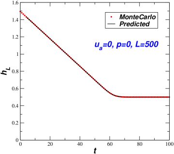
Figure 6: Average height $h_{L}(t)$ as a function of time for the PARPM with $u_{a}=0$, $p=0$ and lattice size $L=500$. The initial configuration is one of the $|N_{0},k\rangle$, with $N_{0}=249$ (see Fig. 5 for notation). The continuous curve is the prediction given by (3.18), and the discrete points are the results obtained from Monte Carlo simulations.

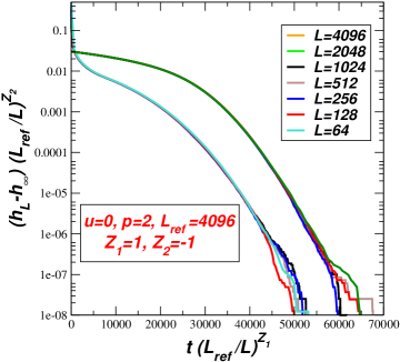
Figure 7: The finite-size scaling of the average height for the PARPM with $u=0$ and $p=p_{c}=2$. The two set of curves correspond to distinct initial conditions. In the lower set the initial configuration is $|N_{0},1\rangle$ (see Fig. 6) where we have $N_{0}=31$ tiles in the first row above the substrate. In the top curves the initial configuration is the one where we have a pyramid whose basis has $N_{0}=31$ in the first row, above the substrate configuration. The parameter $L_{ref}=4096$ was chosen to better present the results and the exponents are $z_{1}=z_{2}=1$.

From (3.14) and (3.15) we can calculate the time dependence of the observables (2.20)-(2.23). The average number of peaks and valleys $\tau_{L}(t)$, heights $h_{L}(t)$ and contact points $K_{L}(t)$ are given by

$$\tau_{L}(t)-\tau_{L}(\infty)=-\frac{2}{L-1}\sum_{k=0}^{N_{0}-1}\frac{(E_{1}t)^{k}}{k!}e^{-E_{1}t},$$ (3.16)

$$(h_{L}(t)-h_{L}(\infty))\frac{L}{2}=K_{L}(\infty)-K_{L}(t)=e^{-E_{1}t}\left\{\sum_{k=0}^{N_{0}-1}(N_{0}-k)\frac{(E_{1}t)^{k}}{k!}\right\},$$ (3.17)

where $\tau_{L}(\infty)=1-\frac{1}{L}$, $h_{L}(\infty)=\frac{1}{2}$ and $K_{L}(\infty)=\frac{1}{2}-\frac{1}{L}$ are the values of these quantities at the final substrate configuration. In both expressions, if $(E_{1}t)^{N_{0}-1}/(N_{0}-1)!>(E_{1}t)^{N_{0}}/N_{0}!$, i.e., $t<t_{0}=N_{0}/E_{1}$, we can approximate the sum by $\exp(E_{1}t)+O((E_{1}t)^{N_{0}}/N_{0})$. This is quite interesting since for times up to $t\mathchar 13358\relax t_{0}$ the exponential decay is totally canceled and the system behaves as if it was gapless. Only for $t\mathchar 13350\relax t_{0}$ the exponential decay will govern the time decay to the stationary state. In Fig. 6 we illustrate this behavior by comparing the average height $h_{L}(t)$ predicted by (3.17) with the results obtained by averaging $3200$ runs of a Monte Carlo simulation for the PARPM with $L=500$ (open ends), with parameters $u_{d}=1$, $p=0$ and having as the initial state the configuration containing $N_{0}=249$ tiles in the first layer above the substrate. The agreement is excellent, as expected. We also see in the figure that up to a transient time $t_{0}=N_{0}/E_{1}$ ($\sim 62$ in this case), $h_{L}(t)$ has a linear time dependence, and for $t\mathchar 13350\relax t_{0}$ the system finally decays to the substrate, where $h_{L}(\infty)=1/2$. This linear behavior is better seen by writing (3.17) as

$$<h_{L}(t)-h_{L}(\infty)>\frac{L}{2}=e^{-E_{1}t}\left\{\frac{N_{0}}{(N_{0}-1)!}(E_{1}t)^{N_{0}-1}+(N_{0}-E_{1}t)\sum_{n=0}^{N_{0}-2}\frac{(E_{1}t)^{n}}{n!}\right\},$$ (3.18)

where the linear behavior dominates up to $t\mathchar 13358\relax t_{0}=N_{0}/E_{1}$.

Let us analyze the time behavior for large lattices and $0<{p}<p_{1}=2$. From (3.3) the gap is finite and given by

$$E_{1}=2u_{p}(2-p+2(p-1)/L).$$ (3.19)

In order to do the limit $L\to\infty$ is necessary to define what are the initial states, as we change the lattice sizes. Two distinct limits give us quite different behavior. In the first one we consider a set of initial states where we have a fixed number of tiles $N_{0}$ above the substrate. In this case we have the linear time behavior up to the finite time $t_{0}=N_{0}/E_{1}$, but for $t\mathchar 13350\relax t_{0}$ the system exhibits its exponential-law decay. In the second case we consider the set of initial states that $N_{0}/L$ is fixed as $L\to\infty$. In this case $t_{0}=N_{0}/E_{1}\to\infty$, and the system behaves at all times as would not be gapped, similarly as happens in a critical system. This unusual and surprisingly behavior happens due to the infinite size Jordan-cell structure for the eigenvalue $E_{1}$ of the Hamiltonian.

Let us now consider the case $p={p_{1}}=2$. In this case we see from (3.19) that the gap vanishes as $E_{1}\sim 1/L$, when $L\to\infty$, and the system is critical. In order to see this critical behavior we must consider, as $L\to\infty$, a sequence of initial states with a fixed number $N_{0}$ of tiles above the substrate. In Fig. 7 we illustrate this critical behavior by considering, for several lattice sizes the average height $h_{L}(t)$ for two distinct sets of initial conditions. In the first one we take as the initial configurations the configurations $|N_{0},1\rangle$ given in Fig. 6, where we have $N_{0}=31$ tiles added in the first row above the substrate, while in the second one we take as initial configurations the ones where we have a pyramid whose basis contains $N_{0}=31$ tiles in the first row above the substrate. As we can see in Fig. 7 for both initial conditions, the curves for the several lattice sizes collapse in the finite-size scaling curve

$$\frac{h_{L}(t)}{h_{\infty}}-1=\frac{1}{L^{\alpha}}f(\frac{t}{L^{z}}),$$ (3.20)

with the dynamical critical exponents $\alpha=z=1$. For $p\geq 2$, the initial states we considered are already absorbing states and the system is already in the stationary state. It is simple to convince ourselves that even if we consider more general initial states, that are not absorbing states, since we have only desorption, after a relatively short time the system is trapped on one of the absorbing states. This means that for $u=u_{a}/u_{d}=0$ we have a phase transition in the PARPM at $p=p_{c}=2$, separating phases with single and multiple absorbing states. [2]. Knowing that $z=1$, we can write from (3.19) the gap $E_{1}\sim L^{-z}g(\Delta^{1/\nu_{\perp}})$, with $\Delta=p-p_{c}$, $z=\nu_{\perp}=1$, that is similar to the results obtained from the numerical diagonalization of the evolution operator of the contact process.

It is important to mention that although $z=1$ the model at $p=p_{c}=2$ is not conformally invariant. From (3.3) we see that, for $L\to\infty$, the gaps behave as $E_{i}\sim A_{i}/L$ with amplitudes $A_{i}=4iu_{d}(2i-1)$. These amplitudes does not give the conformal towers that are expected in the finite-size scaling limit of conformally invariant critical systems.

4 The model with equal rates of adsorption and
desorption

We consider in this section the PARPM for the special case where the absorption and desorption rates are equal, i. e, $u=u_{a}/u_{d}=1$. For this case the model with open boundary condition was studied in [12] for the values of the parameter $0\leq p<{p}_{1}=2-\frac{1}{L}$. The model is conformally invariant for $0\leq p<{p}_{1}$, with a $p$-dependent sound velocity. At $p={p}_{1}$ the substrate configuration becomes an absorbing state and is the stationary state. However, the system stays during a time interval which grows exponentially with the lattice size, in a quasi-stationary state with the same properties ($z=1$) as the conformal invariant phase $0<p<{p}_{1}$ of the model.

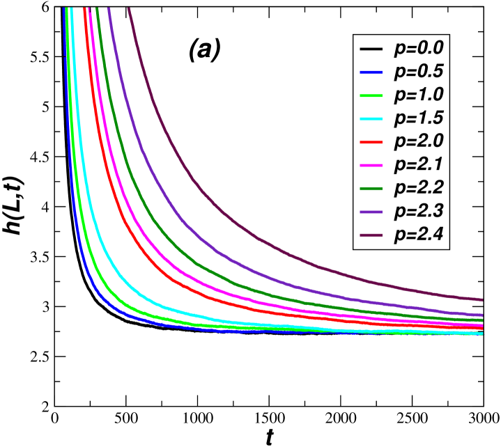
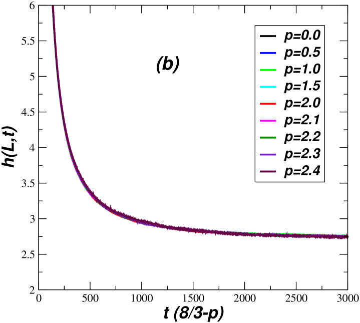
Figure 8: (a) Values of the average height $h_{L}(t)$ for the PARPM with $L=8192$ sites and open boundary conditions. The curves are for several values of the parameter $p$ and $u=1$. (b) Same as (a) but the time is now scaled by the factor $(8/3-p)$, which is proportional to the sound velocity.

We now consider the case where $p>{p}_{1}$. In Fig. 8a we show the time evolution of the average height $h_{L}(t)$ for the model with open boundary conditions, lattice size $L=8192$ and some values of $p$. In Fig. 8b we show that these curves, similarly as happens for $p<{p}_{1}$ [9], are collapsed in a single universal curve by re-scaling the time scale by a factor proportional to the sound velocity of the model $t\to t(\frac{8}{3}-p)$. Similar curves are also obtained for the other observables defined in (2.22)-(2.23). This is a surprise, since for $p>{p}_{1}$, as $p$ increase the number of absorbing states increases drastically. For $L\to\infty$, although the system has an infinite number of absorbing states, it stays in a quasi-stationary state with similar properties as the conformally invariant systems ($0\leq p<{p}_{1}$). The system prefers (independent of the value of $p$) to stay in configurations with number of peaks smaller than those of the absorbing states, and the net effect of the parameter $p$ is just a change in the time scale. To illustrate, we show in Fig. 9 the average distribution of heights $h_{L}(x)$ at site $x$ for the model in the quasi-stationary state. The data are for $L=8192$ sites, open boundary conditions and the values of $p=0,1$ and $2.1$. We see a nice collapse of the curves regardless $p<{p}_{1}$ or $p>{p}_{1}$. We also show in the figure (circles) the predicted curve [10] for the standard $u=1$ RPM:

$$h(L)=\gamma\ln[L\sin(\pi x/L)/\pi]+\beta,$$

with $\gamma=\sqrt{3}/2\pi\approx 0.2757$ and $\beta=0.77$. The coefficient $\gamma$ can be derived exploiting the conformal invariance of the model [11, 10]. We verified that the curves collapse up to $p=p_{c}=8/3$. At this point, from (2.19), all the configurations with $3L/8$ peaks are absorbing states, and the time scale disappears (the sound velocity is zero). For $p>p_{c}$ the system decays, after a short time, in one of the infinitely many absorbing states.

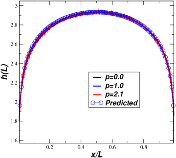
Figure 9: The average distribution of heights at the sites $x$ ($0\leq x\leq L$) in the stationary state of the PARPM with open boundary conditions. The lattice size is $L=8192$, $u=1$ and the parameters $p$ are shown in the figure. The predicted universal curve $h(L)=0.2757\ln[L\sin(\pi x/L)/\pi]+0.77$ is also shown (circles).

In order to calculate the decay time of the quasi-stationary state for ${p}_{1}<p\leq p_{c}$, we need to evaluate the eigenvalues of the Hamiltonian. In Fig. 10 we show the lowest 38 eigenvalues of the Hamiltonian as a function of $p$, for the model with $L=18$ sites and open boundary conditions. We see from this figure that at $p={p}_{1}=\frac{17}{9}=1.888\cdots$ the energy of the eigenstate that is the first excited state for $p<{p}_{1}$ has a large decrease. It degenerates with the ground state ($E_{0}=0$) exponentially with the lattice size, as $L\to\infty$. This is due to the appearance of the absorbing state whose configuration is the substrate, with 9 peaks. At $p={p}_{2}=\frac{17}{8}=2.125$ additional 36 excited states also degenerate with the ground state, since all the configurations with 8 peaks are also absorbing eigenstates. At $p={p}_{3}=\frac{17}{7}\approx 2.428$ additional degeneracies of the ground state happens due to the new absorbing states with 7 peaks. We also verify in Fig. 10 that the lowest gap is much lower in the region $p>{p}_{1}$ as compared with the one in the conformally invariant region $p<{p}_{1}$. In the region $p<{p}_{1}$ we verified from a finite-size extrapolation, using lattice sizes up to $L=28$, that the first excited state, as $L\to\infty$, is given by $E_{1}=E_{1}(p)=2\pi v_{s}(p)/L$ where $v_{s}(p)=9(\frac{8}{3}-p)\sqrt{3}/10$ is the sound velocity, in agreement with the prediction in Ref. [9]. This value of $E_{1}$ for $L\to\infty$ is represented as the dashed line in Fig. 10. The fact that even for $p>{p}_{1}$ the system has similar physical properties as $p<{p}_{1}$ is an indication that most probably the lowest gap above the quasi-stationary state is also given by the same last expression $E_{1}(p)=2\pi v_{s}(p)/L$.

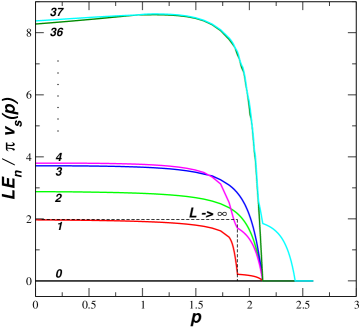
Figure 10: The ground state ($E_{0}$) and the lowest 37 excited eigenenergies, as a function of $p$, of the Hamiltonian of the PARPM, with $u=1$, lattice size $L=18$ and open boundary conditions. In the figure $v_{s}(p)=9(8/3-p)\sqrt{3}/10$ is the sound velocity. The dashed line is the prediction for the first excited state for $p<8/3$ when $L\to\infty$.

For $p\geq{p}_{1}$ it is not possible to obtain reasonable estimates for the lowest gap $E_{1}$, from direct diagonalizations of the Hamiltonian. In this case the finite-size effects are stronger and we need to consider lattices sizes larger than the ones we were able to diagonalize exactly ($L\sim 20$). In this case we extract $E_{1}$ from the time evolution of the average number of peaks and valleys

$$\tau_{L}(t)=\tau_{L}(\infty)[1-a\exp(-E_{1}t)],$$ (4.1)

where $a$ is a constant that depends on the initial condition considered. In order to test the precision of the estimates obtained from (4.1) we compare them with the exact results derived from direct diagonalizations of the Hamiltonian with small lattice sizes and $p={p}_{1}=2$. In table 1 we give the estimates obtained from both methods. As we can see for $L>8$ the difference among the estimated values are less that $1\%$.

In order to estimate $E_{1}$ using larger lattice sizes we chose, for a fixed value of $p=p_{i+1}$, a sequence of lattice sizes $L=L(i)$ such that, from (2.19), $p=(L-b)/(\frac{L}{2}-i)$, with $i$ an integer and $b=0$ or 1 for the periodic or open boundary conditions. For example for $p=2.2$ the lattice sizes are $L(i)=22i$ and $L(i)=12+22(i-1)$ for periodic and open boundary conditions.

$E_{1}(L)$	8	10	12	14	16	18
Exact	0.227	0.139	0.0922	0.0636	0.04481	0.0318
From (4.1)	0.231	0.140	0.0920	0.0638	0.04476	0.0320

Table 1: Estimated results for the lowest gap $E_{1}$ for the PARPM with $u=1$ and $p=2$ and lattice sizes $L=8-18$. In the first row we show the values obtained from the exact diagonalization of the Hamiltonian. In the second row the values are obtained from the large-time fit (using (4.1)) of $5\times 10^{5}$ samples in a Monte Carlo simulation.

In Fig. 11 we show the values obtained for the gap $E_{1}$, for the case of open (Fig. 11a) and periodic boundary conditions (Fig. 11b). The data are for lattice sizes up to $L=18292$. We see from these figures that the leading finite-size scaling behavior of the gap is given by:

$$E_{1}\sim\frac{1}{L^{z}}f(\Delta L^{1/\nu}),$$ (4.2)

where $\Delta=p_{c}-p$, with $p_{c}=8/3$, $z=0.563$ and $\nu=2.103$. We also see from the figure that the scaling function $f(0)\neq 0$ and decreases exponentially with the argument. This imply that the decay time $1/E_{1}$ of the quasi-stationary state increases exponentially as the lattice size increases. For $p>p_{c}$ we verified that the quasi-stationary state disappears and the system is trapped in one of the absorbing states. We then expect that $p=p_{c}$ is a critical point. The PARPM with the values $p={p}_{1}$ and $p={p}_{c}$ seems to be similar to the bimodal and spinodal limits of metastable systems [19]. Considering different values of $u$ for the PARPM we should have as the limiting values $p={p}_{1}=2$ and $p_{c}(u)$ for the region with absorbing sates. For $u=0$ we have seen in Sec. 4 that $({p}_{1},p_{c})=(2,2)$, and in Sec. 6 we are going to see that for $u\to\infty$, $({p}_{1},p_{c})=(2,4)$. We can then reach the critical point ($2,8/3$) at $u=1$ by considering $u\mathchar 13350\relax 1$ with the parameter $p=8/3$ fixed (see Fig. 1). In Fig. 12a this was done for the case of periodic boundaries, and we see that, as in Fig. 11a, the gap behaves as in (4.2). These results imply that at $u=1$ and $p=p_{c}=8/3$, the energy gap has the $L$-dependence $E_{1}\sim 1/L^{z}$, with the dynamical critical exponent $z\sim 0.51-0.57$. To improve this estimate we consider a sequence of periodic lattices with $712\leq L\leq 370944$. The results are shown in Fig. 12b and give us $z=0.561\pm 0.008$.

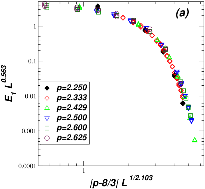
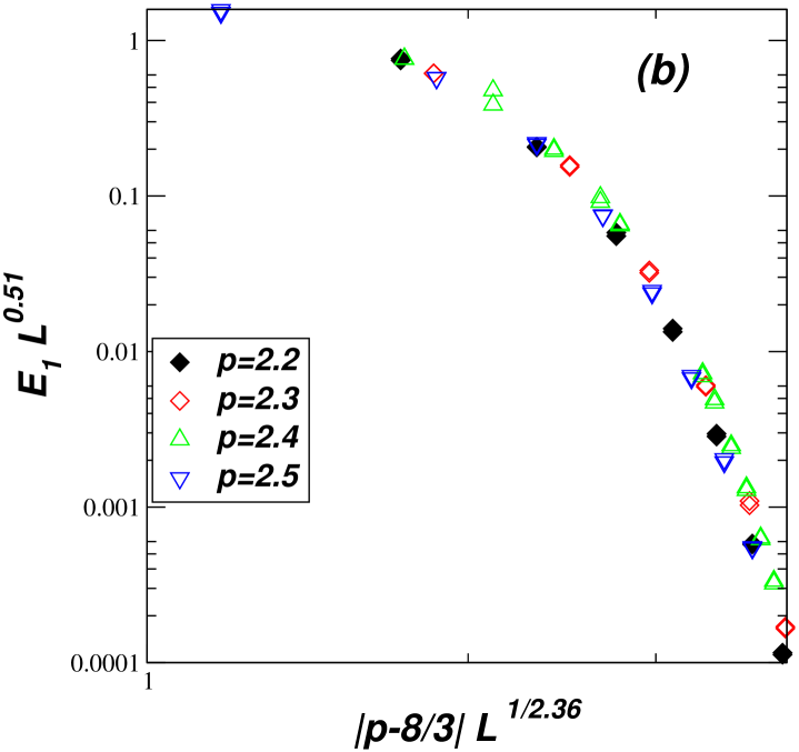
Figure 11: Finite-size scaling for the gap of the PARPM with $u=1$, for several values of $p$ and lattice sizes $L\leq 18292$ (compare with (4.1)). The lattice size values depend on the parameter $p$ (see the text). (a) Open boundary condition. b) Periodic boundary condition.

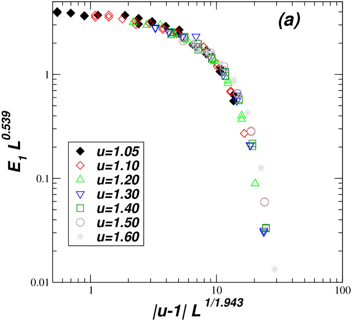
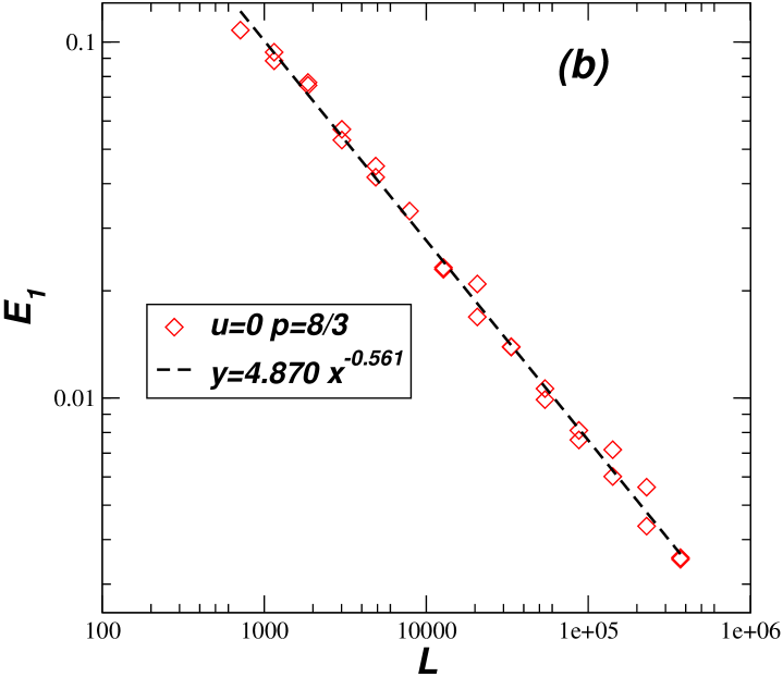
Figure 12: Energy gap $E_{1}$, as a function of $L$, for the PARPM with periodic boundary conditions for the parameter $p=8/3$ and in the region $u\geq 1$. (a) Data collapse using in (4.2) $\Delta=u-u_{c}$, with $u_{c}=1$. The lattice sizes are $104\leq L\leq 54120$. (b) Power-law behavior for the gap at $u=1$. The lattice sizes are $L=8.i$ ($712\leq L\leq 370944$), so that $p=L/(L/2-i)=p_{c}=8/3$.

In summary for $0\leq p<{p}_{1}$ the model is conformally invariant with dynamical critical exponent $z=1$. For ${p}_{1}\leq p<p_{c}$ the model is in a phase containing multiple absorbing states, but these absorbing states are only reached after a time interval that increases exponentially with the lattice size. In this phase the system stays in a quasi-stationary state with dynamical critical exponent $z=1$ and similar properties as in the conformally invariant phase $p<{p}_{1}$. The sound velocity for $0\leq p\leq p_{c}$ is proportional to $(p-8/3)$. At $p=8/3$ it vanishes and we have a new critical behavior with $z=0.561\pm 0.008$. A similar vanishing of the sound velocity happens in the XXZ quantum chain when we approach the ferromagnetic point ($z=1$) coming from the anti ferromagnetic conformally invariant phase ($z=1$) [20]. For values $p>p_{c}=8/3$ the model is frozen in one of the infinitely many absorbing states.

5 The model with no desorption ($u\to\infty$)

We consider in this section the PARPM in the case we have only adsorptions, i. e., $u_{d}=0$ and $u=u_{a}/u_{d}\to\infty$. In the stochastic evolution only the tilted tiles that hit sites with valleys ($h_{i-1}>h_{i}<h_{i+1}$) produce changes in the growing surface ($h_{i}\to h_{i}+2$). This model can be interpreted as a kind of a single step model [21, 22] without desorption.

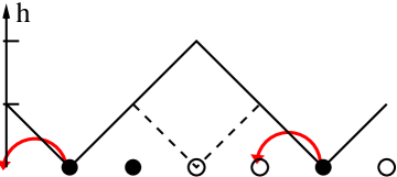
Figure 13: The correspondence among the configurations in the height and the particle-hole representations (circles) in the periodic PARPM. At $u\to\infty$ (no desorptions) the only allowed motions for the particles are shown in the figure.

It is interesting to map the configurations of the PARPM in terms of excluded volume particles and holes in the lattice, as in [13] (particle-hole representation). The particles (holes) are defined on the sites $i$ where $h_{i+1}>h_{i}$ ($h_{i+1}<h_{i}$). In this map the number of particles and holes are equal (see Fig. 13, as an example). The adsorptions in the sites with valleys correspond to the motion of a particle to the leftmost lattice position, provided it is empty (hole). For $u\to\infty$ this is the only allowed motion as happens in the totally asymmetric exclusion process (TASEP) [14, 15]. The PARPM with the choice $p=1$ recovers the standard RPM. In this case all the sites during the stochastic evolution are chosen with equal probability and the particle-hole mapping give us the standard TASEP model [14, 15]. In the case of open boundary conditions the model is noncritical. The stationary state, that corresponds to the pyramid configuration in the height representation is the configuration where the $L/2$ particles are in the left half of the $L$-sites lattice. However for periodic chains the model is critical and belongs to the Kardar-Parisi-Zhang (KPZ) universality class, whose dynamical critical exponent $z=3/2$.

For general values of the parameter $p$ the PARPM with no desorption ($u_{d}=0$) and adsorption rate $u_{a}$ will be related to a generalized TASEP whose transition rates for the particles hoppings depend non locally on the particles positions. As a consequence of our definition (2.7) the transition rates depend on the number of peaks (or valleys) in the height representation of the model. In the particle-hole representation this is the total number $N_{ph}^{c}$ of hole-particle pairs (hole in the left and a particle in the right), or equivalently is the number of particles’s clusters in the configuration. From (2.8) the transition rates for the particles in the generalized TASEP is $u_{a}q_{c}$ where

$$q_{c}=\mbox{Max}\left\{0,\frac{1-\frac{N_{ph}^{c}p}{L}}{1-\frac{N_{ph}^{c}}{L}}\right\},$$ (5.1)

where for $p=1$ we have the standard TASEP with transition rate $u_{a}$.

Since $N_{ph}^{c}=L/2$ is the maximum value, for $0\leq p<2$ the parameter $p$ acts as a nonlocal perturbation in the TASEP ($p=1$). When $p>1$ ($p<1$) the configurations with larger (smaller) number of pairs $N_{ph}^{c}$ are preferred. For $p\geq 2$ this perturbation introduces a new effect. At $p=2$ the two configurations with $N_{ph}^{c}=L/2$ (all the particles occupying the even or odd sites) become absorbing states. As we increase $p\geq 2$, the configurations $c$ with density of pairs $N_{ph}^{c}/L\geq 1/p$ also become absorbing states. For $p>2$ and $L\to\infty$ we have then an infinite number of absorbing states in a model with particle number conservation. This is similar as happen in other models like the Manna model, the conserved threshold transfer process (CTTP) and in the conserved lattice gas (CLG) [1, 3]. However, as we shall see, the phase transition to the frozen state in our model shows a dynamical critical exponent $z\approx 1$, different from the values $z=1.39$ for the Manna model and CTTP and $z=2$ for the CLG [1, 3].

As happened in the case $u=1$ our results indicate that for $0\leq p<{p}_{1}=2$, where the model has no absorbing states the dynamical critical exponent has the same value as in the $p=1$ standard TASEP where $z=3/2$. In the region $2<p<p_{c}$ the model, although having in the thermodynamical limit an infinite number of absorbing states, stays in a quasi-stationary state with the same critical properties as in the KPZ region $0\leq p<2$, i.e., $z=3/2$. The quasi-stationary state for $2\leq p<4$ decays in an absorbing state after a transient time that diverges exponentially with the lattice size of the system. The net effect of the parameter $p$, for $0\leq p<4$ is a change of the sound velocity of the model, that is proportional to $4-p$.

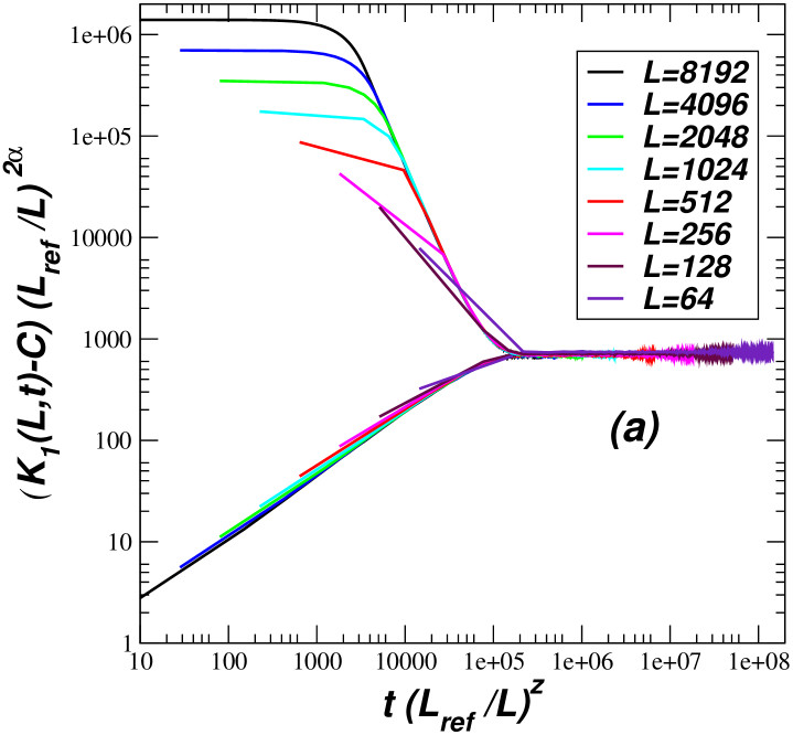
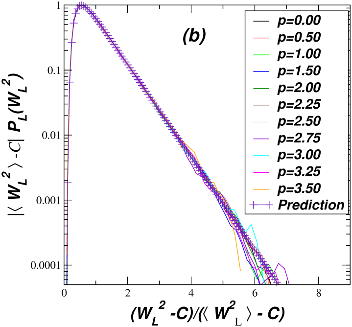
Figure 14: (a) The time evolution of the first cumulant $K_{1}(L,t)$ for the PARPM at $u\to\infty$ and the parameter $p=0.5$, for several lattice sizes. The top curves (bottom curves) are the ones where the initial configuration is the pyramid (substrate). The constant $L_{ref}=8192$ was introduced to better represent the data and $C=0.594$ is obtained as a result of the data collapse of the curves, as the time increases, and by fixing the KPZ exponents $z=3/2$ and $\alpha=1/2$. (b) Probability distribution of the second moment $W_{L}^{2}$ of the height distribution at the stationary ($p<{p}_{1}=2$) or quasi-stationary state ($p>2$) of the PARPM with no desorption ($u\to\infty$). It is also included (crosses) the theoretical KPZ prediction for this distribution [23].

In order to identify the universality class of the PARPM for general values of $p$ and $u_{d}=0$ we calculate the time evolution of the surface roughness

$$W_{L}(t)=\sqrt{\frac{1}{L}\sum_{i=1}^{L}(h(i,t)-\bar{h}(t))^{2}},$$ (5.2)

where $\bar{h}(t)=\frac{1}{L}\sum_{i}h(i,t)$ is the average height of the configuration at time $t$. In Fig. 14a we show the time evolution of the first cumulant of $W_{L}^{2}$, i. e., $K_{1}(L,t)=<W_{L}^{2}(t)>$, for the model with $p=0.5$. We consider as the initial conditions the configurations with a single peak (top curves) and $\frac{L}{2}$ peaks (bottom curves). The collapse of the curves in the infinite-size limit

$$<W_{L}(t)>\sim L^{\alpha}f(t/L^{z}),$$ (5.3)

give us $z=3/2$ and $\alpha=1/2$, indicates that the model belongs to the KPZ universality class of critical behavior. We also consider, for the lattice size $L=4096$, the probability distribution of $W_{L}^{2}$ in the stationary states for $p<{p}_{1}$, and also for ${p}_{1}\leq p<p_{c}$. This is shown in Fig. 14b. We also include in this last figure the theoretical prediction for the KPZ model [23] (crossed points). We clearly see a nice agreement, indicating that indeed for $0\leq p<p_{c}$ the model belongs to the KPZ universality class, where $z=3/2$ and $\alpha=1/2$. For all cases the probability distribution behaves as

$$P_{L}(W_{L}^{2})=\frac{1}{<W_{L}^{2}>-C}f\left(\frac{W_{L}^{2}-C}{<W_{L}^{2}>-C}\right),$$ (5.4)

where $C=0.594$ is a finite-size correction and $<\cdot>$ is the standard average over the configurations [24].

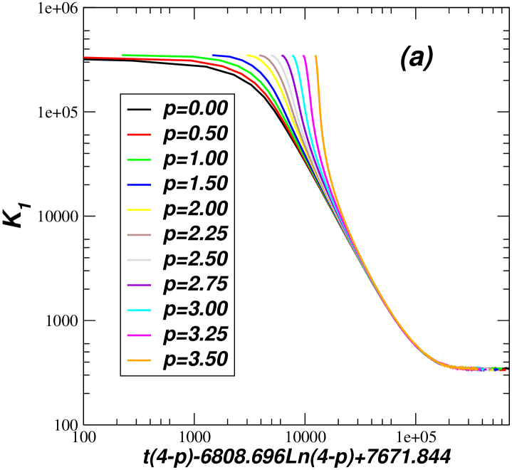
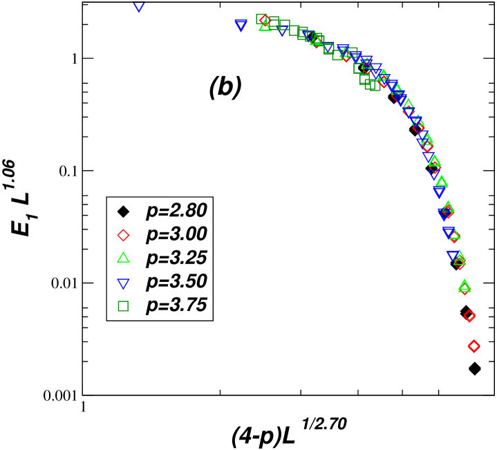
Figure 15: (a) The time evolution of the first cumulant $K_{1}(L,t)=<W_{L}^{2}>$ for the PARPM at $u\to\infty$ with several values of the parameter $p$ (shown in the figure) and for the lattice size $L=4096$. As time grows the curves collapse if the time is scaled by the factor $4-p$. (b) Finite-size scaling for the gap of the PARPM at $u\to\infty$, for several values of $p<4$. The gaps were estimated by fitting ($1-\tau/\tau_{\infty}$) with (4.2) and $\Delta=4-p$.

We want now to consider the limiting case $p=p_{c}=4$. In Fig. 15a we show the time evolution, for several values of $p<p_{c}$, of the average $K_{1}(L,t)$ for the lattice size $L=4096$. We see from the figure that the time scale changes as a function of $p-4$. We also notice the existence of a transient regime, that increases as we get closer to $p_{c}$. This is an indication that at $p_{c}$ the system may have a distinct behavior. In order to verify this possibility we need to evaluate the lowest gap $E_{1}$ for $p<p_{c}$. As we did in Sec. 4 for the case $u=1$, this gap could be calculated from the large-time dependence of the observable $\tau_{L}(t)$ (see (4.1)). In Fig. 15b we show the finite-size scaling obtained for the gap at $u\to\infty$.

In Fig. 16a we show in a semi-log plot the quantity $1-\tau_{L}(t)/\tau_{L}(\infty)$, starting with the system in the pyramid configuration. We clearly see from this figure that the exponential time dependence (4.1) is only obtained for short times. As we obtained in the $u=0$ case (see Sec. 3), if the eigenvalue $E_{1}$ has an associated Jordan-cell structure we may have instead of a simple exponential decay as in (4.1), the more general time dependence

$$1-\frac{\tau_{L}(t)}{\tau_{L}(\infty)}\sim t^{n}\exp(-E_{1}t),$$ (5.5)

where $n$ is an $L$-dependent integer and $E_{1}$ is the gap. In Fig. 16b we fit, using (5.5), the results obtained for the lattice $L=25552$. We obtained a good fitting for $t>5\times 10^{5}t$ giving us the value $E_{1}=1.81\times 10^{-4}$ and $n=85$. Repeating the same fitting for the lattice sizes $L=3728$, $6032$, $9760$ and $15792$ we obtain $E_{1}\sim 1/(0.22L-87.81)$ and $n\sim 0.213L^{0.59}$. This result indicates that indeed at $p=p_{c}$ we have a new critical behavior with the dynamical critical exponent $z=1$. From Fig. 16a we see that the simple exponential as in (4.1) give us the short-time behavior. Extracting the gap from the initial times, assuming (4.1) for the small lattices $208\leq L\leq 2304$ we obtain $E_{1}\sim 1/(0.66L-11.07)$. These results together with the ones obtained by using the fitting (5.5) for large times are shown in Fig. 17. There is however an apparent contradiction in these results since the gap calculated from the large time decay is greater than the one governing the short-time behavior. This is an indication that indeed at large times the lowest gap $E_{1}$ appearing in (5.5) should be replaced by a higher excited state $E_{i}>E_{1}$. This means that the Jordan-cell structure dominating the $n$-polynomial behavior at large times is not associated to the first excited state, but to a higher excited state. The large dimension of the Jordan cells associated to $E_{i}$ are enough to kill the exponential decays associated to the smaller gaps.

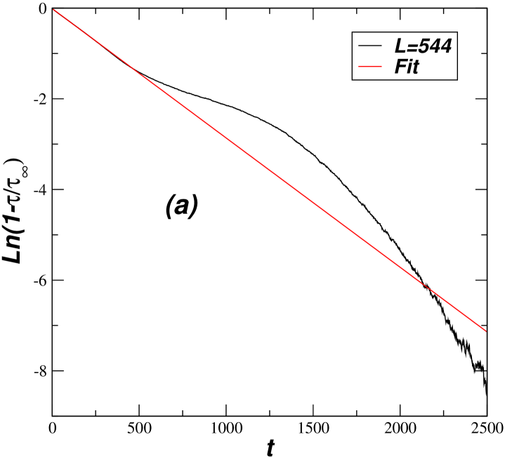
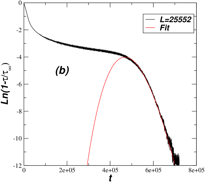
Figure 16: (a) Semi-log plot of the ratio $\tau_{L}(t)/\tau_{L}(\infty)$ (black curve),as a function of time, for the periodic PARPM with $L=544$ sites, no desorptions ($u\to\infty$) and at the critical point $p_{c}=4$. The initial state of the system is the pyramid configuration. The red line is the linear fit obtained for $t<500$, as expected from (4.1). (b) Same as in (a) with the larger lattice size $L=25552$. The curve in red is obtained by fitting, according to (5.5), the data for the larger times $t>5\times 10^{5}$.

In summary for $u=\infty$ the PARPM is in the KPZ universality class ($z=3/2,\alpha=1/2$) for all the values of $0\leq p<p_{c}=4$. For $2<p<p_{c}$, although there exist an infinite number of absorbing states, the system stays during a time interval that grow exponentially with the lattice size, in a quasi-stationary state sharing the critical properties of the KPZ universality class. For $0\leq p<p_{c}$ the large-time behavior has a simple exponential decay with a time decay $1/E_{1}$. However at $p=p_{c}=4$ our results indicate that a Jordan-cell structure associate to a higher gap $E_{i}>E_{1}$, dominates the large-time behavior. In this case the system stays in a quasi-stationary state with a dynamical critical exponent $z\approx 1$. For $p>p_{c}$ the model is in a frozen state, i.e., after a short time decays to one of the infinitely many absorbing states.

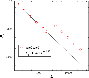
Figure 17: The gap estimates obtained from the time dependence of $\ln[1-\tau_{L}(t)/\tau_{L}(\infty)]$ of the PARPM with periodic boundaries, $u\to\infty$ and $p=p_{c}=4$. For $t<1500$ the estimates were obtained from the fitting with (4.1) and for large times the fitting was done by using (5.5).

6 Conclusions

The peak adjusted raise and peel model (PARPM) was studied in this paper. The model can describe the interface fluctuations of a growth model (height representation) or the particle density fluctuations in a nonlocal particle-hole exclusion process (particle-hole representation). The model has two parameters: $u$ and $p$. The parameter $u\geq 0$ controls the ratio between the rates of adsorption and desorption in the height representation, and in the particle-hole representation it gives the relative weight among the local and nonlocal hoppings of the particles. The parameter $p\geq 0$ distinguish, during the time evolution, the configurations according to the number of peaks, in the height representation, or the number of particle-hole pairs in the particle-hole representation. In the bulk limit ($L\to\infty$), for any value of $u$ and $p>2$, the model has an infinite number of absorbing states. An schematic phase diagram of the model is shown in 1. We study the model with open and periodic boundary conditions by choosing some special values of $u$ and general values of $p$.

a) At $u=0$ (Sec. 3) where we have no desorption in the height representation, the model is gapped for $p<2$, having an absorbing state as the stationary state. In the bulk limit the associated Hamiltonian has an infinite dimensional Jordan cell structure associated to the first excited state. Starting from some simple configurations we were able to derive the analytical time dependence of some observables for arbitrary time. Interestingly, if we consider in the $L\to\infty$, a sequence of initial configurations where the density of tiles in the first row is fixed and nonzero, the system stays an infinite time before decaying into the final absorbing state and, does not fell the system’s gap. At $p=2$ however, the model is critical with a dynamical critical exponent $z=1$. For $p>2$ the stationary state is one of the infinitely many absorbing states.

b) For $u=1$ we extend the results obtained in [9, 12] for $p\leq 2$, where the model is known to be conformally invariant (central charge $c=0$ and $z=1$). Our results show that for $2\leq p<8/3$, where the model has an infinite number of absorbing states, it stays in a critical quasi-stationary state during a time interval that grows exponentially with the lattice size. The quasi-stationary state has the same critical properties as the conformally invariant phase $p<2$. At $p=p_{c}=8/3$ our results give us a new critical behavior with dynamical critical exponent $z\sim 0.561$. For $p>p_{c}=8/3$ the system, after a short time, stays inactive in one of the infinitely many absorbing states. The phase transition at $p_{c}=8/3$ separates an active phase from an inactive phase of a system with an infinite number of absorbing states. We think that is the first time we see such a phase transition, i.e., a transition to a frozen inactive state coming from a critical phase, that although having infinitely many absorbing states, is ruled by an active quasi-stationary state.

c) For $u\to\infty$ the model has no desorption and it loses part of its non locality, since the adsorptions are local. In the particle-hole representation the model is equivalent to a TASEP where we have $L/2$ particles that can hop to the next-neighbor site at the left, provided it is empty (hole). For a given value of the parameter $p$ the rate of the hopping process depends on the number of particle-hole pairs in the configuration. In this limit the model is gapped or not depending if the boundary condition is open or periodic, respectively. At $p=1$ the motion of the particles are independent of the numbers of particle-hole pairs and the model recovers the standard critical TASEP with the dynamical critical exponent $z=3/2$ of the KPZ universality class. Our results indicate that for all values $0\leq p<p_{c}=4$, the model has the same critical behavior as the KPZ universality class. For $2\leq p<p_{c}=4$, similarly as happened in the case $u=1$, the model although having an infinite number of absorbing states, survives for a time interval that diverges exponentially with the lattice size, in a critical quasi-stationary state whose critical properties are the same as the ones on the region without absorbing states ($0\leq p<2$). At $p=p_{c}=4$, as in the cases $u=0$ and $u=1$, the model shows a new critical behavior with dynamical critical exponent $z=1$. We also noticed that this new critical behavior is a consequence of large dimensional Jordan cells associated not to the first excited state, but to a higher excited one.

To conclude it is interesting to see the PARPM as a generalized asymmetric exclusion process ASEP [15], with nonlocal jumps of excluded volume particles (controlled by $u$) whose rates are biased (controlled by $p$) by the number of particle-hole pairs in the configurations. The parameter $u$ is relevant since it changes the critical behavior. The parameter $p$, on the other hand, is irrelevant up to $p=p_{c}(u)$ ($p_{c}(0)=2,p_{c}(1)=8/3,p_{c}(\infty)=4$), although for $2\leq p\leq p_{c}(u)$ there exist an infinite number of absorbing states. At $p=p_{c}(u)$ the model has a new critical behavior with a $u$-dependent critical exponent $z=z(u)$.

7 Acknowledgments

We would like to thank José Abel Hoyos and Vladimir Rittenberg for useful discussions and a careful reading of the manuscript. This work was support in part by the Brazilian funding agencies: FAPESP, CNPq and CAPES.

References

-
[1]
SchmittmannB and Zia R K P, 1995 Phase Transitions and Critical
Phenomena vol 17, ed C Domb and J Lebowitz (London: Academic)
Halpin-HealyT and Zhang Y-Ch., 1995 Phys. Rep 254 215
Ódor G 2008 Universality in nonequilibrium lattice systems (World Scientific) - [2] Hinrichsen H 2000 Advances in physics 49 815–958
- [3] Henkel M, Hinrichsen H, Lübeck S and Pleimling M 2008 Non-equilibrium phase transitions vol 1 (Springer)
- [4] Edwards S F and Wilkinson D R, 1982 Proc. R. Soc. A 381 17
-
[5]
Kardar M, Parisi G and Zhang Y-C 1986 Phys. Rev. Lett. 56 889
Halpin-Healy T and Zhang Y-C, 1995 Phys. Rep. 254 215 -
[6]
De Gier J, Nienhuis B, Pearce P A and Rittenberg V 2004 J. Stat.
Mech. 114 1–35
Alcaraz F C, Levine E and Rittenberg V 2006 J. Stat. Mech. P08003
Alcaraz F C and Rittenberg V 2007 J. Stat. Mech. P07009
Alcaraz F C, Pyatov P and Rittenberg V 2008 J. Stat. Mech. P01006 - [7] Razumov A V and Stroganov Yu G 2001 J. Phys. A: Math. Gen. 34 3185
- [8] https://en.wikipedia.org/wiki/Catalannumbers
- [9] Alcaraz F C and Rittenberg V 2010 J. Stat. Mech. P12032
-
[10]
Alcaraz F C, Rittenberg V and Sierra G 2009 Phys. Rev. E 80 030102(R)
Alcaraz F C and Rittenberg V 2010 J. Stat. Mech. P03024 - [11] Jacobsen J L and Saleur H 2008 Phys. Rev. Lett. 100 087205
- [12] Alcaraz F C and Rittenberg V 2011 J. Stat. Mech. 2011 P09030
- [13] Alcaraz F C and Rittenberg V 2013 J. Stat. Mech. 2013 P09010
- [14] Derrida B, Evans M and Mukamel D 1993 J. Phys. A: Math. Gen. 26 4911
- [15] Derrida B and Mallick K 1997 J. Phys. A: Math. Gen. 30 1031
- [16] Pearce P A, Rasmussen J and Tartaglia E 2004 J. Stat. Mech. P05001
- [17] Morin-Duchesne A and Saint-Aubin Y 2013 J. Phys. A: Math. Gen. 46 494013
- [18] Family F and Vicsek T 1985 J. Phys. A: Math. Gen. 18 L75
- [19] Debenedetti P G 1996 Metastable liquids: concepts and principles (Princeton University Press)
- [20] Alcaraz F C, Barber M N and Batchelor M T 1988 Ann. Phys.(NY) 182 280
- [21] Barabási A L and Stanley H E 1995 Fractal concepts in surface growth (Cambridge university press)
- [22] Sasamoto T and Spohn H 2010 Phys. Rev. Lett. 104 230602
- [23] Antal T, Droz M, Györgyi G and Rácz Z 2002 Phys. Rev. E 65 046140
- [24] Oliveira T and Reis F A 2007 Phys. Rev. E 76 061601