Eigenvalue Dependence of Numerical Oscillations in Parabolic Partial Differential Equations

Abstract.

This paper investigates oscillation-free stability conditions of numerical methods for linear parabolic partial differential equations with some example extrapolations to nonlinear equations. Not clearly understood, numerical oscillations can create infeasible results. Since oscillation-free behavior is not ensured by stability conditions, a more precise condition would be useful for accurate solutions. Using Von Neumann and spectral analyses, we find and explore oscillation-free conditions for several finite difference schemes. Further relationships between oscillatory behavior and eigenvalues is supported with numerical evidence and proof. Also, evidence suggests that the oscillation-free stability condition for a consistent linearization may be sufficient to provide oscillation-free stability of the nonlinear solution. These conditions are verified numerically for several example problems by visually comparing the analytical conditions to the behavior of the numerical solution for a wide range of mesh sizes.

1. Introduction

Numerical methods are useful for constructing quick estimates of solutions to partial differential equations (PDEs). Error can, however, creep into the solution making results inaccurate and, at times, physically meaningless due to stability issues. Yet, ensuring the stability of the numerical solution to a well-posed PDE ensures convergence to the true solution of the PDE. Von Neumann [4] provided an analytical method for determining the stability of linear numerical schemes, which he refined from the stability analysis provided first by Crank and Nicolson [3]. Numerical oscillations can also occur, either as a small noise in the solution or as dramatic swings in the solution leading to an instability. Scientists have long been concerned with these oscillations, but have most often responded by damping all oscillations. For example, Britz et al. [5] developed a damping algorithm specifically for oscillations caused by discontinuous initial conditions for the Crank-Nicolson scheme based off the initial work by ï¿œsterby [6]. But simply damping these oscillations can change the nature of the solution itself, especially if the solution was naturally oscillatory to begin with. Rather, if we understand the nature of these oscillations and can identify why they occur, then we can avoid them altogether.

Previous work by Harwood [12] suggests there exists a more restrictive condition for oscillation-free conditions as noted by the eigenvalues of the time-step matrix. A spectral analysis would be appropriate to determine the appropriate conditions on the scheme, providing a necessary and sufficient condition for oscillation-free solutions.

Nonlinear problems provide a different challenge, but a consistent linearization technique could provide insight through spectral or Von Neumann analyses. Such PDEs have a range of application. Each of these models are prone to oscillation given certain conditions. This paper investigates the relationship between eigenvalues and oscillatory behavior and proposes necessary and sufficient conditions for oscillation-free stable numerical solutions.

2. Theory

2.1. Numerical Convergence

Convergence of a numerical solution to the exact solution of a given PDE is paramount to implementing a numerical method, but this form of convergence is hard to measure. Instead, a numerical method can be proven convergent indirectly by showing it to be consistent and stable. A numerical method is consistent if it converges to the given PDE as the step size all go to zero. Further, a method is stable if any errors are bound instead of being magnified.

Definition 1.

A two-level difference scheme, $U^{n+1}=MU^{n},$ is said to be stable with respect to the norm $||.||$ if there exist positive constants $\triangle t_{0},\ and\ \triangle x_{0},$ and non-negative constants K and $\beta$ so that

$$||U^{n+1}||\leq Ke^{\beta\triangle t}||U_{0}||,$$

for $0\leq t=(n+1)\triangle t,\ 0<\triangle x\leq\triangle x_{0}\ and\ 0<\triangle t\leq\triangle t_{0}$.

Since $||U^{n+1}||\leq||M^{n+1}||\cdot||U_{0}||$, $||M^{n+1}||\leq Ke^{\beta\Delta t}$ is sufficient for stability of the solution. To compensate for $\rho(M^{n+1})\leq||M^{n+1}||_{2}$ we force the Von Neumann criterion

(2.1) $$\rho(M)\leq 1+C\triangle t,$$

for some $C\geq 0$, so that $\rho(M^{n+1})\leq 1+C(n+1)\triangle t\leq Ke^{C(n+1)\triangle t}$, which is a necessary condition for stability. If the matrix is symmetric, $\rho(M^{n+1})=||M^{n+1}||\leq 1+C(n+1)\triangle t\leq e^{C(n+1)\triangle t}$, then the criterion is necessary and sufficient. Often $C=0$ is adequate to ensure a necessary and sufficient condition for stability, but with exponentially growing solutions, the Von Neumann criterion may require $C>0$. Solving for the amplification factor, $e^{\gamma\Delta t}=\frac{U_{m}^{n+1}}{U_{m}^{n}}$. The condition is applied such that $|e^{\gamma\triangle t}|\leq 1+C\triangle t$. However, if the eigenvalues are easily calculated, we can determine more accurately the stability and behavior of the solution.

Theorem 2.

Lax-Richtemeyer Theorem:

“Given a Partial Differential Equation and a consistent numerical method, a numerical method is convergent iff it is stable.”

And more specifically, for two-level numerical method, this can be restated as the Lax Equivalence theorem :

Theorem 3.

Lax Equivalence Theorem:

“A consistent, two-level difference scheme, $u^{n+1}=MU^{n}+\triangle t\cdot G^{n}$, for a well-posed linear (constant-coefficient) initial-value problem is convergent if and only if it is stable.”

Using consistent schemes, we can explore the stability bounds to indirectly verify convergence. Burden and Faires [2] define stability for a numerical system as:

2.2. Spectral Analysis

For linear PDEs, the eigenvalues of the transformation matrix indicate the stability of the solution and evidence suggests they also determine oscillatory behavior. Since $\rho(M)\leq||M||_{2}$, an analysis of the eigenvalues relates to the boundedness of the solution through the matrix [11]. Assuming that the solution to difference scheme is separable, we can show that the discrete error growth factors are the eigenvalues of M. Also, assuming the solution is separable, as is common for linear PDEs, the eigenvalues can be defined by:

(2.2) $$e^{\gamma\Delta t}\equiv\frac{\epsilon_{m}^{n+1}}{\epsilon_{m}^{n}}=\frac{U_{m}^{n+1}}{U_{m}^{n}}=\frac{T^{n+1}}{T^{n}}=\lambda,\ \mbox{where }U_{m}^{n}=X_{m}T^{n}.$$

This shows that when separation of variables can be assumed in the PDE, the eigenvalues of the matrix for the numerical scheme equals the error growth factor. This relationship is supported by the similarity of Von Neumann stability analysis to the Matrix Convergence Theorem proven in [10]:

Theorem 4.

(Matrix Convergence Theorem)$\lim_{n\rightarrow\infty}M^{n}$ exists iff $|\lambda_{i}|<1$ or $\lambda_{i}=1,\ \forall i$ and the multiplicity of $\lambda=1$ is equal to the dimension of the eigenspace, $E_{1}$.

Furthermore, $lim_{n\rightarrow\infty}M^{n}$ is bounded iff $|\lambda|\leq 1$ when $mult(1)=dim(E_{1})$ [10]. Because of this connection, a spectral analysis of the transformation matrix can reveal patterns in the orientation, spread, and balance of the growth of errors for various wave modes and unbalanced eigenvalues can lead to oscillations in the results.

These troublesome oscillations have several sources. Unstable oscillations stem from unstable methods, where the algorithm is either inconsistent or the discretization is too large. Other sources are discontinuities: in the initial condition, or between the initial condition and boundary condition. The Crank-Nicolson method can be susceptible to these discontinuities, which propagate oscillations (stable and unstable) in a normally consistent and stable method. The nature of the PDE itself can create oscillations, but these are generally more acceptable since these are expected and are part of the solution. However, we are concerned with stable oscillations. Theoretically, oscillations are hard to define. From a physical study of springs, one can define oscillations as a type of periodic movement or displacement from an equilibrium position [7]. While this is visually descriptive, it is lacking analytically. Mathematically defining oscillations is difficult, but numerically describing them can be easier. Since oscillations displace positively and negatively from the equilibrium, we implemented a working numerical definition for oscillation. By tracking the sign of the displacement, we could track if the signs of the spatial components flipped in time. Pearson [8] and Britz et al. [5] stated that preserved monotonicity in time could suggest oscillation-free behavior for a solution. While not an exact definition of oscillation, monotonicity provides a sufficient condition for oscillation-free stability. Thus, we used a theoretical definition for temporal monotonicity: $U_{m}^{n+1}\leq U_{m}^{n}$ or $U_{m}^{n+1}\geq U_{m}^{n}$ . Spatial monotonicity is defined in a similar manner where the lower index changes instead.

With this information, if a region of stable oscillations were to exist for a particular scheme, then it would have to be bounded above by the stability condition (obviously, since we wish to account for oscillations inside the stability bounds) and bounded below by the monotonicity condition.

Tridiagonal matrices create a very interesting special case. Each equation we investigated, under Dirichlet boundaries, created a tridiagonal matrix of a form whose eigenvalues were calculated by [12]. Furthermore we could reasonably restrict the eigenvalues further to an oscillation free condition, by forcing the real parts of the eigenvalues positive [12]. For notation, we will refer to the upper off diagonal entries as $a$, the diagonal as $b$ and the lower off diagonal as $c$. For such tridiagonal matrices, the eigenvectors with first component $u_{i}^{(1)}=\sin\left(\frac{i\pi}{N+1}\right),\ \forall i$, are defined by their $k^{th}$ component as:

$$u_{i}^{(k)}=\sin\left(\frac{ik\pi}{N+1}\right),\ \forall i$$

This method is effective in a spectral analysis of Dirichlet boundary conditions. The explicit Euler Heat equation is a prime example for tridiagonal matrices. In the explicit Heat Equation $a=c$, thus the eigenvalues and eigenvectors are independent of a square root and the equation is quickly simplified. Also note that in the Heat FTCS scheme, $b=1-2r$, where $r=\frac{\triangle t}{\triangle x^{2}}$. This means that the upper bound on the eigenvalues is 1, which is the upper bound to stability. We can calculate these eigenvalues with:

$$\lambda_{i}=1-4r\sin^{2}\left(\frac{i\pi}{2(N+1)}\right)$$

where $N$ is the size of the matrix.

By calculating the max and min we can definitively say that $\lambda_{i}\in(1-4r,1)$ but as $r$ increases in size, the eigenvalues leak into the negative real parts causing oscillations. Thus we can use eigenvalues to more restrictively bound oscillation-free stability. Other boundaries can change the nature of the matrix and make calculating the eigenvalues difficult. Neumann problems rid us of our tridiagonal assumption, making eigenvalues more difficult to analyze. In these cases, since we can assume a linear separable solution, the Von Neumann error factor can be used to determine the behavior of the eigenvalues. In analyzing the Heat Crank-Nicolson scheme matrix, a spectral analysis of the eigenvalues showed that Dirichlet problems for the Heat equation lie in the set $\lambda_{i}\in\left[\frac{1-2r}{1+2r},1\right)$. However the Neumann problem showed that the largest eigenvalue was always 1. This meant that Dirichlet problems could experience oscillations if the eigenvalues were to become negative, but all Neumann problems were going to be stable, regardless of the step sizes used for discretization.

2.3. Linearized Analysis of Nonlinear Problems

For nonlinear problems, we wished to investigate three main methods of calculating a numerical solution. An explicit scheme which doesn’t require any linearization but is very susceptible to numerical oscillations as well as instability due to the nonlinearities. A semi-implicit scheme allows us to explicitly solve for the linear portions of the equation, but tackle the nonlinearities implicitly. This creates problems computationally since the matrix requires updates in order to implicitly solve the nonlinearities, making it very costly to constantly update and resume solving. Instead, an implicit scheme which employs a linearization makes computation easier. For one technique, we chose a linear approximation of the nonlinear term:

(2.3) $$f(U_{m}^{n+1})\approx f(U_{m}^{n})+\triangle U\cdot\frac{\partial f(U^{n})}{\partial u}+....\approx f(U^{n})+(U^{n+1}-U^{n})\cdot f_{u}(U^{n})+...$$

This technique aims to approximate the nonlinear pieces independently, similar to the manner used for the finite differences schemes (both are based off of Taylor Series). Because this requires no updates and runs alongside the normal computation, we can solve this linearization scheme relatively easily. Our second technique is a nonlinear freezing technique, where we separate off a linear term from the nonlinear and treat the rest of the nonlinear term as a coefficient. For example, the Fisher-KPP equation:

$$u_{t}=u_{xx}+u(1-u)$$

we use an implicit scheme to get:

$$U_{m}^{n+1}-U_{m}^{n}=r(U_{m+1}^{n+1}-2U_{m}^{n+1}+U_{m}^{n+1})+\Delta t\cdot U_{m}^{n+1}(1-U_{m}^{n+1})$$

Then by freezing the nonlinearity we get:

$$U_{m}^{n+1}-U_{m}^{n}=r(U_{m+1}^{n+1}-2U_{m}^{n+1}+U_{m}^{n+1})+\Delta t\cdot U_{m}^{n+1}(1-\tilde{U})$$

Now that the nonlinearity is frozen, it is treated as some constant coefficient, and we estimate it by using a worst-case bounding for the solution. Determining the use of the maximum or minimum of the matrix $U$ depends on which makes the magnitude of the error factor greatest in the spectral analysis, Nonlinear freezing may be easier computationally, but by only bounding the solution, there is chance that the solution could contain stable oscillations.
Performing stability analysis requires the same techniques as used on a linear PDE plus an analysis of the error created to linearize the PDE. In this way we define stability conditions, oscillation free conditions and balanced eigenvalue conditions which we can compare to those used on linear problems.

Theoretical analysis provides us with a base which we can use to launch our numerical analysis from. Next, we will explain how we used what we knew theoretically, and how we applied that knowledge to create simulations with strong and sound tests, to accurately falsify or confirm our conjectures.

3. Methodology

During simulation, we wished to check three main components: Is the solution stable? Do positive eigenvalues dominate the matrix? And do oscillations appear in the solution? Creating numerical systems to check these conditions challenged us to use definitions for each of these components and implement them. Using the conditions provided by the theoretical analysis, we checked to see if the numerical tests measured up to each of these conditions. In our first steps, we numerically verified that the methods were consistent and usable with Linear PDEs. Using explicit, implicit, and semi-implicit numerical methods, we ran simulations on each numerical scheme for each equation By beginning with Linear PDEs we could develop sound methods which we could apply to more complicated nonlinear equations, after a linearization was applied.

3.1. Stability

Using Burden and Faire’s definition of stability (1), a Von Neumann analysis appropriately prescribed a condition for each scheme. Numerically tracking stability required us to cap the growth of the solution. Burden and Faires used the standard $l_{2}$ norm, but considering the computational strain it required, we sought for a better fit. We settled on the infinity norm (also known as a supremum norm) which is defined by the magnitude of the largest component of the matrix. We will prove that $||U^{n+1}||_{\infty}\leq||M^{n+1}||_{2}||U_{0}||_{2}$, which means that the infinity norm is a tighter condition than an $l_{2}$ norm, making it a necessary condition for stability.

Lemma 5.

$||U^{n+1}||_{\infty}\leq||M^{n+1}||_{2}||U_{0}||_{2}$

Proof.

We will prove this lemma by simplifying the right hand side. For a two-level difference scheme (Def. 1),

$$||M^{n+1}||_{2}||U_{0}||_{2}\geq||M^{n+1}U_{0}||_{2}=||U^{n+1}||_{2}$$

By definition of the 2-norm,

$$||U^{n+1}||_{2}^{2}=\sum_{m=1}^{m}(U_{m}^{n+1})^{2}\geq(U_{k}^{n+1})^{2}\ \forall k$$

which implies that

$$\sum_{m=1}^{m}(U_{m}^{n+1})^{2}\geq\max_{k}(U_{k}^{n+1})^{2},$$

which in turn implies that

$$||U^{n+1}||_{2}=\sqrt{\sum_{m=1}^{m}(U_{m}^{n+1})^{2}}\geq\sqrt{\max_{k}(U_{m}^{n+1})^{2}}=\max_{k}|U_{k}^{n+1}|=||U^{n+1}||_{\infty}.$$

Thus,

$$||U^{n+1}||_{\infty}\leq||M^{n+1}||_{2}||U_{0}||_{2},$$

so the infinity norm provides a tighter bound (3.1) ∎

Realizing that when M is powered up over each temporal step, we prescribed a numerical threshold on the growth of the matrix, U. At first, it seemed appropriate to track the norm of the solution vector U, but M’s growth implies the growth of U, i.e.

$$||U^{n+1}||_{\infty}\geq K||U_{0}||_{2}\mbox{ for }K\gg 1\implies||M^{n+1}||\geq K\gg 1$$

Tracking the matrix multiplier this way, allows us to cap the solution before it gets too big because we know that it is unstable.

3.2. Numerical Oscillations

Oscillations are very hard to track numerically. It requires knowing the behavior of a solution and then finding a manner to track things different than the prescribed behavior. The theoretical monotonicity condition (4) helped us develop a numerical monotonicity check. This definition allowed us to detect oscillations in several initial boundary value problems. A dispersion and dissipation analysis, allowed us to determine the PDE’s natural monotonic behavior (if it behaved monotonically), and thus we could prescribe a monotonicity test which would most appropriately detect oscillations. From our theoretical definition we developed the following numerical test:

(3.1) $$sign(U_{m}^{n+2}-U_{m}^{n+1})*sign(U_{m}^{n+1}-U_{m}^{n})\geq 0$$

By comparing the signs of differences between two previous temporal or spatial steps (depending on the behavior of the solution), we could determine if any oscillations occur by a “flip-flopping” of signs across an equilibrium position.
Our numerical test face some limitations with other PDEs. The Fisher-KPP failed the monotonicity check since, with most initial conditions, there is a diffusive stage before the wave can propagate. We are unable to differentiate physical waves from numerical oscillations by analyzing the solution itself, but have found that eigenvalues of the method can indicate such behavior well.

3.3. Eigenvalues

Preliminary investigation through simulations showed a correlation between positive dominant eigenvalues (a single large positive eigenvalue dominating the behavior of the matrix) and oscillation-free solutions. Since the eigenvalues of the matrix directly relate to the growth factor (2.2), we can conclude that if all of the eigenvalues are positive and have magnitude less than or equal to 1, we know that the solution will be stable and oscillation-free. This provides a lower bound on the oscillation-free condition, which we denote by calculating when $Re(\lambda_{i})>0.$ Qualitatively, we noticed as well that there was a positive and negative balance between eigenvectors for simulations of our Heat FTCS scheme. If a negative eigenvalue had a corresponding positive eigenvalue with approximately equal magnitude, their eigenvectors also correspond in magnitude. This lead us to believe that there existed an oscillation free condition when the eigenvalues must be balanced, or positively dominant, which we track numerically by calculating $\max(Re(\lambda_{i}))-\max(|Re(\lambda_{i})|)\geq 0$. We can calculate if there exists an eigenvalue greater in magnitude (but negative) than the maximum.

3.4. Equations for Analysis

We focused on bounded PDEs which presented Initial Boundary Value Problems (IBVPs), using Neumann and Dirichlet boundary conditions. We began running simulations with linear PDEs to create a foundation for nonlinear PDEs. Two second order spatial PDEs were chosen–Heat Equation and the Linear Reaction-Diffusion Equation. After initial results and analysis were mostly completed on linear PDEs we selected a couple nonlinear equations for analysis: Nonlinear Reaction-Diffusion and Fisher-KPP Equation. Each of these has a variety of nonlinear terms which would allow us to find patterns in the effectiveness of the linearizations.
We chose very simply three basic schemes for numerical analysis of the linear PDEs: an explicit scheme with Forward Euler, an implicit scheme using Backward Euler, and the time averaging Crank-Nicolson. These schemes are all very simple and relatively inexpensive to calculate. The Crank-Nicolson provides the advantage that, through the time averaging,
To tackle the nonlinear equations, we used similar schemes, but replaced Crank-Nicolson with a Semi-Implicit scheme. To effectively calculate the solution, we employed two forms of linearization. First, we used a Nonlinear Freezing technique. This breaks up the nonlinear terms into a linear term with the nonlinear factor treated as a constant coefficient, or frozen in time. This requires matrix updates for the estimations and can be very expensive computationally. For the second, we used a linear approximation method (2.3)which we can use to create an estimation for the nonlinear term. This is a computationally simple task, that tends to be very accurate, and promised to be the best estimator for each of the non-linear terms.

3.5. Program Algorithm

We used MATLAB for our analysis. Our primary program ran simulations for a range of $\triangle x$ and $\triangle t$ values such that $\Delta t,\Delta x\in[0.01,1]$. Nested for-loops stepped through each successive $\triangle x$ value and $\triangle t$ value. For each simulation, our program numerically tested for stability, positively dominated eigenvalues and oscillations (each test is described in their sections), storing each result in a binary matrix. Each equation with its respective scheme had a separate MATLAB file, which contained its matrix (or linearized matrix for the non-linear problems) and their theoretical conditions. After collecting this information and running the simulations, the primary analyzer compiles a visual output, color coded by which conditions were met–from red, meaning unstable, to dark blue, for oscillation-free (see Figure 4.1). The visual also graphed the theoretical and analytical condition curves, which allowed us to compare the numerical data with analysis data. Using another loop, we had the analyzer run through every single scheme file we produced for each of the equation’s numerical schemes.

4. Results

While our main analyzer function provides the majority of the experimental data, we used other simulation programs to visualize the solution located in a specific region on the main analyzer’s visual output. If we required further investigation, we simply exported the $\triangle x$ and $\triangle t$ values and ran the simulation for the scheme. The numerical evidence verified our conjectures. Below is a summary table for each of the equations and schemes we investigated and their results.

Heat Equation ($U_{t}=U_{xx}$)

The Heat Equation was our most basic equation that we focused on, and most of the results from the other equations vary predictably from the initial results presented here.We analyzed the equation and ran simulations using both Neumann and Dirichlet boundary conditions under the three main schemes. The explicit scheme for the Heat Equation produces the most quintessential picture. Each region beneath the stability curves is filled with a color corresponding to each of the expected conditions with a solid blue beneath the monotonicity condition and a small amount of unstable oscillations (marked by yellow) above it, turning into complete instability (marked by red) above. Using these simple linear PDEs we were able to test some of our numerical checks to see if they aligned with our analysis and their conditions.
The Heat Equation’s implicit scheme produced little of interest. Our numerical analysis predicted unconditional stability, and picture was consistent to our prediction, by a completely dark blue window. However, the Crank-Nicolson method produced a very intriguing picture.

The linear front (as seen in Figure 4.2), where stable oscillations began to form puzzled us. Considering that all of the analytical conditions were quadratic in nature due to the numerical schemes, we struggled to find an explanation for the linear front presented by the numerical analysis, since for every other file our tests performed suitably. Additionally, none of the analysis predicted the existence of stable oscillations forming in this particular scheme. Further efforts to devise a possible explanation should be made in the future.

Linear Reaction-Diffusion Equation ($U_{t}=U_{xx}-U$)

The Linear Reaction Diffusion differs only slightly from the Heat Equation. A reaction term makes the solution collapse to the end state much quicker, but not much else is changed otherwise. The analyzer program provided the exact same results as the Heat Equation. Reaction-Diffusion FTCS produced a beautiful spread of color each underneath their expected conditions, with the BTCS complete unstable and curious regions of oscillations occurring behind a linear front on the Crank-Nicolson scheme.

Nonlinear Reaction-Diffusion Equation ($U_{t}=U_{xx}-U^{2}$)

Under a stable and consistent linearization technique, the Nonlinear Reaction-Diffusion Equation behaves exactly like its linear cousin. Under a purely explicit scheme, the equation has nearly identical stability behavior to the linear version. Our analysis showed that with just a numerical estimation of the Non-Linear term in an explicit scheme, reasonable step-sizes can produce accurate and oscillation-free results. Using a Semi-Implicit scheme produced curious results. While stability was assured, oscillations still crept into the solution making this method unreliable.

Nonlinear Fisher-KPP Equation ($U_{t}=U_{xx}+(1-U)\cdot U$)

The Fisher Equation provides the greatest variance from the initial linear model of the Heat Equation. The Fisher Equation provided difficulties in tracking monotonicity and oscillations, considering the nature of the solution containing physical waves in 2D as well as diffusive then expansive behavior in single dimensional space. But with manual investigation, we found that there were stable oscillations that occurred between the balanced eigenvalue condition and the loose Von Neumann condition.

Below is a summary table of each of the equations with the results from each scheme included.

Possible Stability and Oscillatory Behaviors
for given equation and scheme

Key: U - Unstable, SO - Stable Oscillations, OFS - Oscillation Free Stable

Linear Equation	FTCS	CN	BTCS
Heat/Diffusion	OFS, U	OFS, SO	OFS
Linear Reaction Diffusion	OFS, SO, U	OFS	OFS

Nonlinear Equation	FTCS	Semi-Implicit	BTCS w/ Freeze	BTCS w/ LinApprox
Nonlinear Reaction Diffusion	OFS, SO, U	OFS	OFS	OFS
Fisher-KPP	OFS, U	OFS	OFS	OFS

The figures for our files are compared by scheme and represent, the Heat Equation, Nonlinear Reaction Diffusion Equation, and the Fisher-KPP Equation, respectively.

Figure 4.1.

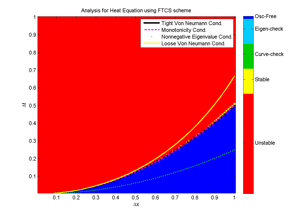
Figure 4.2.

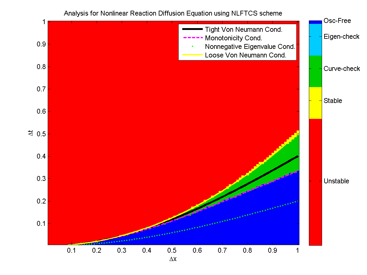
Figure 4.3.

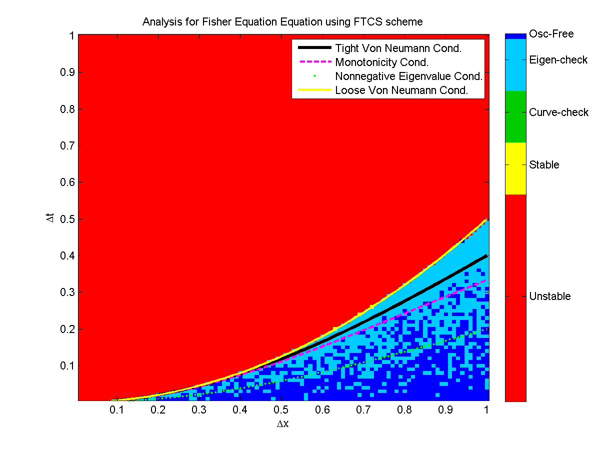
Figure 4.4.

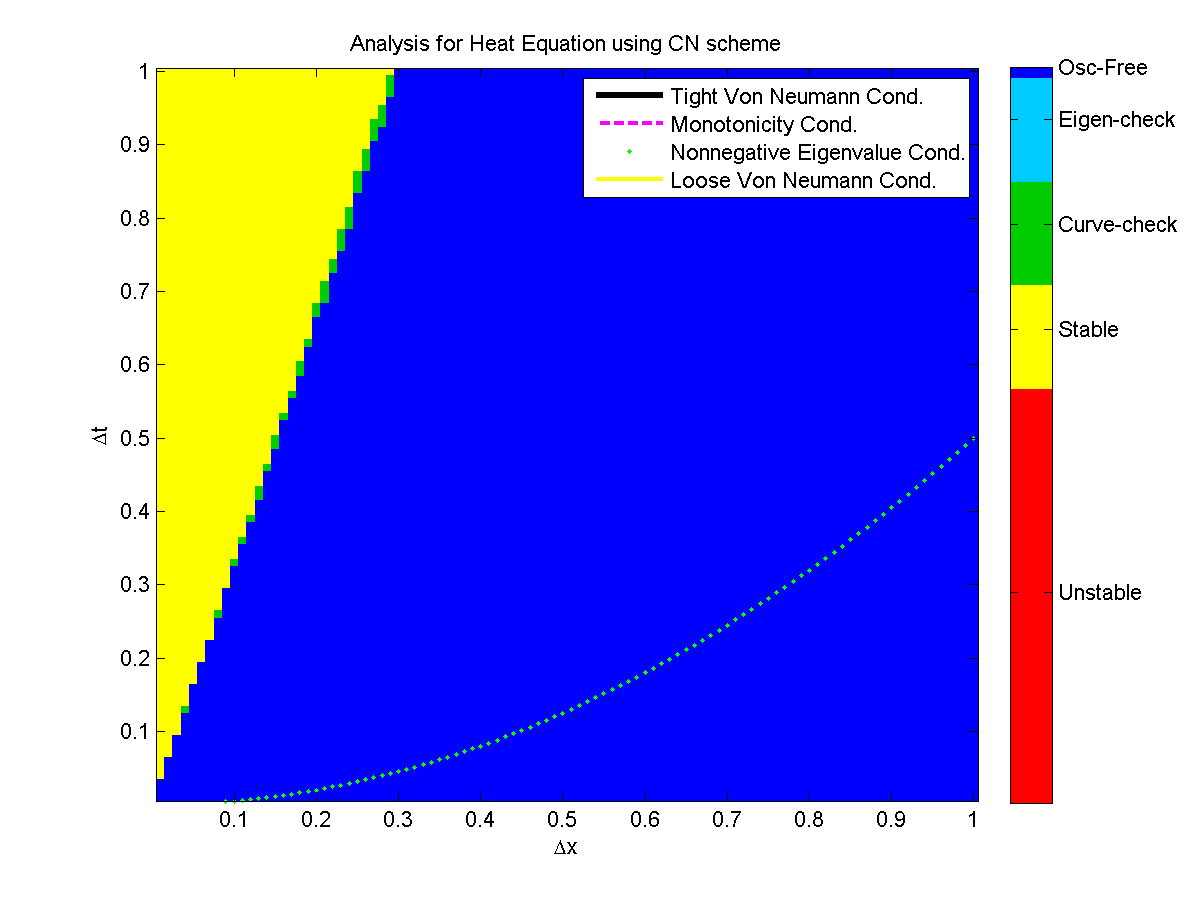
Figure 4.5.

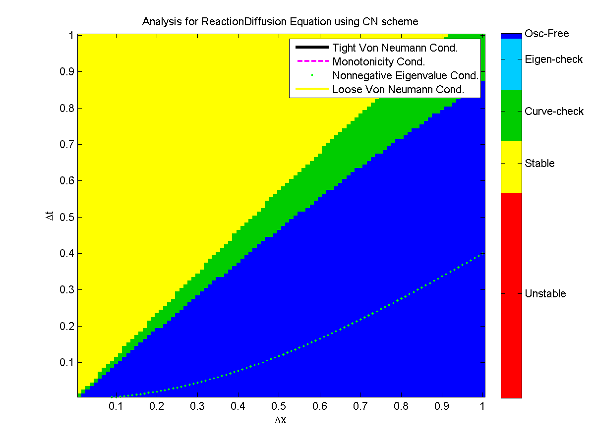
Figure 4.6.

5. Discussion

The diagnosis of numerical oscillations is important, since eliminating them can provide accurate representations of these descriptive and powerful equations, which are incredibly useful to us. The eigenvalues of linear problems provide a concrete connection to the stability and oscillations conditions of numerical schemes, and with a spectral analysis, we can force a condition on the real parts of the eigenvalues remaining positive. More usefully however is the connection between eigenvalues and the Von Neumann error factor, especially in semi-linear or non-linear PDEs. This error factor is a powerful tool in estimating the eigenvalues of these nonlinear PDEs. The following conjectures, backed up by numerical evidence, demonstrate that a consistent linearization of a problem may allow us to form conditions on the linearized scheme using the error factor. Thus, we would be able to contain these oscillations for nonlinear parabolic PDEs as well.

Conjecture 6.

Given a linear PDE with a symmetric positive difference scheme matrix, if there exists a region of numerically stable oscillations, it is bounded below by the positive eigenvalue condition

From preliminary investigation, a relation between the balance of eigenvalues and the monotonicity condition seems evident, most particularly from our data from the Heat FTCS analysis (see Figure 4.1). In analyzing the eigenvalues and eigenvectors, we noticed that if there were paired eigenvalues of similar magnitude by opposite sign, then the eigenvectors were of equal magnitude but opposite sign. This led us to a believe that the balance of these eigenvalues along with their eigenvectors had a place in an oscillation free condition. The balanced eigenvalues and eigenvectors seemed to “block” oscillations.

Conjecture 7.

Given a linear PDE with a well posed scheme and consistent scheme matrix, the solution will be oscillation-free iff there exists a dominating positive eigenvalue.

The numerical evidence for this is very convincing, since the monotonicity condition relates directly to this balanced eigenvalue condition. We have seen this in our numerical results, which is summarized in the Results section along with the visual representation of our data.

Conjecture 8.

Given a nonlinear partial differential equation, the stability and oscillation-free conditions for a consistent linearized form of a nonlinear numerical method is sufficient to ensure oscillation-free stability.

Tying this to the monotonicity condition leads us to the final conjecture. We believe that if a non-linear PDE is monotonic, then it is also oscillation-free. Since the monotonicity condition is a necessary condition on the eigenvalues of a method as well as the fact that it is sufficient for stability, then we believe that the solution will be oscillation-free and stable.

Conjecture 9.

Given a nonlinear partial differential equation with monotonic initial and asymptotic behavior, a numerical method is oscillation-free if it is monotonic. Further, this monotonicity condition matches the oscillation-free condition of the linearized form of the numerical method.

Containing oscillations in Initial Value Boundary Problems, which contain no physical oscillations, remained relatively easy, but exploration of those containing physical waves and oscillations, accurately damping numerical oscillation requires more refined investigation.

References

- [1] Thomas, J.W. “Texts in Applied Mathematics: Numerical Partial Differential Equations, Finite Difference Methods”. Springer-Verlag, 1995. Vol 22, pg. 74.
- [2] Burden, Richard L. and J. Faires, “Numerical Analysis.” Brooks, Cole Cengage Learning, 2011. Ninth Edition. pg. 34.
- [3] Crank, J., and P. Nicolson. "A Practical Method for Numerical Evaluation of Solutions of Partial Differential Equations of the Heat-conduction Type." ACMS University of Arizona. University of Arizona, n.d. Web. 25 June 2013.
- [4] CHARNEY, J. G., FJORTOFT, R. and Von NEUMANN, J. (1950), Numerical Integration of the Barotropic Vorticity Equation. Tellus, 2: 237–254. doi: 10.1111/j.2153-3490.1950.tb00336.x
- [5] D. Britz, O. Osterby, J. Strutwolf, Damping of Crank–Nicolson error oscillations, Computational Biology and Chemistry, Volume 27, Issue 3, July 2003, Pages 253-263, ISSN 1476-9271, http://dx.doi.org/10.1016/S0097-8485(02)00075-X. (http://www.sciencedirect.com/science/article/pii/S009784850200075X)
- [6] Osterby, Ole. "Five ways of reducing the Crank–Nicolson oscillations." BIT Numerical Mathematics 43.4 (2003): 811-822.
- [7] Peterson, Gary L., and James S. Sochacki. Linear Algebra and Differential Equations. Boston: Addison-Wesley, 2002. Print.
- [8] Pearson, Carl. “Impulsive End Condition for Diffusion Equation.” AMS, Mathematics of Computation, 19 : 570-576. ISSN 1088-6842 (online). http://www.ams.org/journals/mcom/1965-19-092/S0025-5718-1965-0193765-5/S0025-5718-1965-0193765-5.pdf
- [9] Lui, S.H. “Numerical Analysis of Partial Differential Equations.” John Wiley and Sons, 2011. First Edition.
- [10] Friedberg, Stephen H., Arnold J. Insel and Lawrence E. Spence.”Linear Algebra.” Prentice Hall, Pearson Education, Inc. Fourth Edition.
- [11] Horn, Roger A. and Charles R. Johnson. “Matrix Analysis.” Ports & Telecom Press, 2005. Second Edition. ## include either this one or Friedberg
- [12] Harwood, Richard C. “Operator Splitting Method and Applications for Semilinear Parabolic Partial Differential Equations.” Diss. Washington State University. 2011. PDF.