A split step Fourier/discontinuous Galerkin scheme for the Kadomtsev–Petviashvili equation

Abstract

In this paper we propose a method to solve the Kadomtsev–Petviashvili equation based on splitting the linear part of the equation from the nonlinear part. The linear part is treated using FFTs, while the nonlinear part is approximated using a semi-Lagrangian discontinuous Galerkin approach of arbitrary order.

We demonstrate the efficiency and accuracy of the numerical method by providing a range of numerical simulations. In particular, we find that our approach can outperform the numerical methods considered in the literature by up to a factor of five. Although we focus on the Kadomtsev–Petviashvili equation in this paper, the proposed numerical scheme can be extended to a range of related models as well.

1 Introduction

The Kadomtsev–Petviashvili (KP) equation has been proposed in [17]. It models wave propagation in dispersive and nonlinear media and is usually stated as follows

$$(u_{t}+6uu_{x}+\epsilon^{2}u_{xxx})_{x}+\lambda u_{yy}=0,$$ (1)

where $\lambda$ and $\epsilon$ are parameters. Although it is most well known to model the propagation of water waves [1] it has found applications in such diverse areas as ion-acoustic plasma waves [17, 22], the semiclassical description of motion for lattice bosons [9], and waves in compressible hyperelastic plates [5]. From a mathematical point of view the equation can be understood as a two-dimensional generalization of the Korteweg–de Vries equation (KdV) equation and it shares many interesting properties, such as soliton solutions and blow-up in finite time [20, 18, 19, 21], with that system.

It has been found that solving the KP equation poses significant challenges for numerical methods. While it is clear that explicit schemes suffer from a very severe stability restriction on the time step size (due to the third order derivative in space), it was found in [18] that implicit and implicit-explicit (IMEX) methods often do not converge (i.e. that the iterative linear or nonlinear solvers necessary for the efficient implementation of these schemes do not converge). Thus, exponential integrators have been suggested and successfully applied to the KP equation [18]. However, it has been realized recently that splitting schemes can be competitive especially in the low to medium precision regime most of interest in applications. The reason why splitting methods have been dismissed up to that point is that no efficient schemes were available to solve the Burgers’ type nonlinearity. In [13] this problem was solved by using a semi-Lagrangian method based on Lagrange interpolation. Nevertheless, employing Lagrange interpolation is perhaps the most significant weakness of that algorithm. It is well known that Lagrange interpolation is quite diffusive (see, for example, [25, 14]) which is certainly not ideal taking the Hamiltonian structure (i.e. dissipation free nature) of the KP equation into account. This is in particular true as for the exponential integrators (pseudo) spectral methods can be used in the nonlinear part as well.

In the context of the Vlasov equation semi-Lagrangian methods have a long tradition. In recent years, semi-Lagrangian discontinuous Galerkin methods have been studied extensively as these methods provide a local approximation (which facilitates parallelization) and are only slightly diffusive (see [23, 7, 24, 13, 11, 12, 6, 26, 2]). However, in this case only constant advection problems have to be solved. Position dependent problems have been considered both in the context of kinetic problems [8, 23] and in the context of tracer-particle transport phenomena [16, 4]. Some of these techniques have also been extended to second order equations [3]. A nonlinear problem with a constant advection has been considered in [2]. Let us duly note, however, that in all of the mentioned works the advection is still linear.

In the present paper we propose a semi-Lagrangian discontinuous Galerkin method for a nonlinear advection problem (more specifically, Burgers’ equation) that is used within a time splitting approach to solve the KP equation. The proposed algorithm can take arbitrarily large steps in time with only a very modest increase in the run time. The algorithm as well as some computational aspects are described in section 2. We then investigate the performance of the proposed method by conducting numerical simulations for a range of problems (section 3). Finally, we discuss some directions of future work and conclude in section 4.

2 Description of the numerical method

We consider the KP equation as stated in equation (1). In accordance with the literature we choose either $\lambda=1$ (weak surface tension) or $\lambda=-1$ (strong surface tension) and call the latter the KP I model and the former the KP II model.

Before a numerical scheme is applied we rewrite equation (1), assuming periodic boundary conditions, in evolution form

$$u_{t}+6uu_{x}+\epsilon^{2}u_{xxx}+\lambda\partial_{x}^{-1}u_{yy}=0,$$ (2)

where $\partial_{x}^{-1}$ is understood as the regularized Fourier multiplier of $-i/k_{x}$. That is, we use the Fourier multiplier

$$\frac{-i}{k_{x}+i\lambda\delta}$$

with $\delta=2^{-52}$ (the machine epsilon for double precision floating point arithmetic). In this work, as in [18], only classical solutions of the KP equation will be considered.

As a first step, we split equation (2) into a linear part

$$u_{t}=Au=-\epsilon^{2}u_{xxx}-\lambda\partial_{x}^{-1}u_{yy}$$ (3)

and a nonlinear part

$$u_{t}=B(u)=-6uu_{x}.$$ (4)

The former is solved using fast Fourier transform (FFT) techniques (we denote the solution for the initial value $u^{0}$ at time $\tau$ as $\mathrm{e}^{\tau A}u^{0}$). The numerical method proposed for the latter is described in detail in the remainder of this section (we denote the solution for the initial value $u^{0}$ at time $\tau$ as $\varphi_{\tau}^{B}(u^{0})$).

Before proceeding, let us emphasize that even if the solution to equation (2) is sufficiently regular, shocks (i.e. discontinuous solutions) can develop as equation (4) is integrated in time. Since our algorithm for Burgers’ equation is not equipped to handle such discontinuous solutions, this imposes a restriction on the step size $\tau$. Note, however, that this is not a CFL condition as the restriction only depends on properties of the solution (and not on the grid size). In any case, numerical simulations conducted in [13] show that for the KP equation, the problem we are ultimately interested in, this is not an issue. More precisely, the step size is dictated by accuracy constraints and we are able to take comparable or even larger time steps to what has been reported in the literature (for exponential integrators or implicit numerical methods, see for example [18]).

In the present work we will exclusively use the second order accurate Strang splitting scheme

$$u^{n+1}=\mathrm{e}^{\frac{\tau}{2}A}\varphi_{\tau}^{B}(\mathrm{e}^{\frac{\tau}{2}A}u^{n}),$$

where $u^{n}$ is an approximation to the exact solution $u(t^{n})$ at time $t^{n}=n\tau$. Let us note, however, that in [13] extensions to fourth order splitting methods have been discussed as well.

2.1 The semi-Lagrangian discontinuous Galerkin approach for the nonlinearity

Our goal in this section is to compute an approximation to the nonlinear part of the splitting procedure (given in equation (4)). That is, we consider Burgers’ equation

$$\partial_{t}u(t,x)+u(t,x)\partial_{x}u(t,x)=0,\qquad\qquad u(0,x)=u^{0}(x).$$

By using the method of characteristics (see, for example [27]) we obtain

$$X^{\prime}(t;t^{n+1},x) =U(t;t^{n},u^{0}(X(t^{n};t^{n+1},x)))$$

$$U^{\prime}(t;t^{n},u^{0}(x)) =0,$$

where $X(t;s,x)$ and $U(t;s,u)$ are the characteristic curves of the position and the solution, respectively, that satisfy $X(s;s,x)=x$ and $U(s;s,u)=u$. Note that since $x$ is known at time $t^{n+1}$ and $u^{0}$ is known at time $t^{n}$ we have to integrate $X$ backward in time and $U$ forward in time. However, since $U$ is constant in time we immediately obtain

$$U(t;t^{n},u^{0}(x)) =u^{0}(x)$$

which implies that

$$X^{\prime}(t;t^{n+1},x)=u^{0}(X(t^{n};t^{n+1},x)).$$ (5)

Therefore, we have eliminated $U$ and the desired solution of Burgers’ equation can be written as

$$u(t,x)=u^{0}(X(t^{n};t^{n+1},x)).$$ (6)

We still have to integrate $X$ (starting from $x$) backward in time in order to obtain the solution at $x$ (i.e. we have to solve equation (5)). However, since the right hand side is constant we can rewrite this differential equation as an algebraic equation

$$X(t^{n};t^{n+1},x)=x-\tau u^{0}(X(t^{n};t^{n+1},x)),$$ (7)

where $\tau=t^{n+1}-t^{n}$ is the time step size. Note that obtaining a unique solution of equation (7) is predicated on the assumption that the characteristics do not cross.

The most straightforward approach to compute an approximate solution of (7) is by conducting a fixed-point iteration. That is, we perform the following iteration

$$\alpha^{(k+1)}=x-\tau u^{0}(\alpha^{(k)}),\qquad\qquad\alpha^{(0)}=x.$$

Until now we have left space continuous. Thus, the only approximation made is due to the truncation of the fixed-point iteration. However, in order to implement a viable numerical scheme on a computer, a space discretization strategy has to be employed. As stated in the introduction we will perform the space discretization in the context of the semi-Lagrangian discontinuous Galerkin (sLdG) approach.

First, we divide our computational domain $[a,b]\subset\mathbb{R}$ into a number of cells $I_{i}=[x_{i-1/2},x_{i+1/2}]$ with size $h=x_{i+1/2}-x_{i-1/2}$. For simplicity, we only consider an equidistant grid here. However, the method described can be extended easily to the case of varying cell sizes. In the $i$th cell the function values at the points $x_{ij}$ are stored, where $x_{ij}=a+h(i-1/2+\xi_{j})$ and $\xi_{j}$ is the $j$th Gauss–Legendre quadrature node scaled to the interval $[0,1]$. The index $j$ runs from $0$ to $k$, where $k$ is the polynomial degree that is used in each cell (note that $o=k+1$ is the formal order of this approximation). Within this discretization an approximation of the analytic solution is expressed as follows

$$u^{n}(x)=\sum_{ij}u_{ij}^{n}\ell_{ij}(x),$$ (8)

where $\ell_{ij}$ is the $j$th Lagrange polynomial in cell $I_{i}$ based on the nodes $x_{i0},\dots,x_{ik}$ (i.e. the Gauss–Legendre quadrature nodes scaled and shifted to the $i$th cell). Note that this setup implies that $u_{ij}\approx u(x_{ij})$ (i.e. the degrees of freedom of the numerical scheme are approximations to the function values at the Gauss–Legendre quadrature nodes in each cell).

Now, we have to determine the coefficients at the next time step $u_{ml}^{n+1}$ from the coefficients $u_{ml}^{n}$. We start by multiplying the solution of (6) with $\ell_{ml}$ and integrate in order to obtain

$$\int_{I_{m}}u^{n+1}(x)\ell_{ml}(x)\,\mathrm{d}x=\int_{I_{m}}u^{n}(X(t^{n};t^{n+1},x))\ell_{ml}(x)\,\mathrm{d}x$$

which yields

$$\frac{h\omega_{l}}{2}u_{ml}^{n+1}=\int_{I_{m}}u^{n}(X(t^{n};t^{n+1},x))\ell_{ml}(x)\,\mathrm{d}x,$$

where $\omega_{l}$ are the quadrature weights. That is, we perform a projection of the analytic solution to the subspace of polynomials up to degree $k$ (in each cell). Evaluating this integral is not as straightforward as one might assume at first. This is due to the fact that the function $u^{n}$ is discontinuous and a direct application of Gauss–Legendre quadrature (or any other quadrature rule for that matter) would not give the (up to machine precision) exact result.

To remedy this situation we proceed as follows. First, we use (8) to write

$$u_{ml}^{n+1}=\frac{2}{h\omega_{l}}\int_{I_{m}}u^{n}(X(t^{n};t^{n+1},x))\ell_{ml}(x)\,\mathrm{d}x=\frac{2}{h\omega_{l}}\sum_{ij}u_{ij}^{n}\int_{I_{m}}\ell_{ij}(x^{b})\ell_{ml}(x)\,\mathrm{d}x,$$ (9)

where $x^{b}=X(t^{n};t^{n+1},x)$ is used as a shorthand to denote endpoint of the characteristic starting at $x$. Now, only a small minority of integrals in the sum will contribute a non-zero value to $u_{ml}^{n+1}$. To identify the indices $i$ for which this is true, we have to determine to what extend the support of $\ell_{ij}(x^{b})$ overlaps with $I_{m}$. There are two possibilities of nonempty intersection that we handle separately in the implementation of our numerical scheme:

• Full overlap ($\text{supp}\;\ell_{ij}(x^{b})\supset I_{m}$): In this case the function $\ell_{ij}(x^{b})$ is polynomial in $I_{m}$ and we can apply a Gauss–Legendre quadrature rule in order to compute the integral exactly;

• Partial overlap: In this case the function $\ell_{ij}(x^{b})$ has one or two discontinuities in the interval $I_{m}$. In this case we apply a Gauss–Legendre quadrature to $\text{supp}\;\ell_{ij}(x^{b})\cap I_{m}$.

To determine which of these cases apply (and in the latter case what the endpoints of integration should be) we follow the characteristics forward in time. That is, to obtain $\text{supp}\;\ell_{ij}(x^{b})=[a_{i},b_{i}]$ we have to compute

$$a_{i}=X(t^{n+1};t^{n},x_{i-1/2}),\qquad\qquad b_{i}=X(t^{n+1};t^{n},x_{i+1/2}).$$

Following the characteristics forward in time is less involved since we now have to solve

$$X^{\prime}(t;t^{n},x) =u^{0}(X(t^{n};t^{n},x))$$

which immediately yields

$$X(t^{n+1};t^{n},x)=x+\tau u^{n}(x).$$

Thus, we have

$$a_{i}=x_{i-1/2}+\tau u^{n}(x_{i-1/2}),\qquad\qquad b_{i}=x_{i+1/2}+\tau u^{n}(x_{i+1/2}).$$ (10)

The difficulty here is that $u^{n}(x_{i-1/2})$ and $u^{n}(x_{i+1/2})$ are not well defined due to the discontinuous approximation used for $u^{n}(x)$. Thus, we replace equation (10) by

$$a_{i}=x_{i-1/2}+\tau\tilde{u}^{n}(x_{i-1/2}),\qquad\qquad b_{i}=x_{i+1/2}+\tau\tilde{u}^{n}(x_{i+1/2})$$ (11)

with

$$\tilde{u}_{i-1/2}^{n}=\frac{u^{n}(x_{i-1/2}+)+u^{n}(x_{i-1/2}-)}{2},$$

here we have used $+$ and $-$ to denote the right-sided and left-sided limit, respectively. The choice made yields the shock speed consistent with the exact solution of the Riemann problem for Burgers’ equation. Note that although the discontinuity is on the order of the approximation error and thus the accuracy of the numerical scheme is not negatively impacted, we will see in section 2.4 that conservation of mass is lost.

In principle, we could use equation (9) as the basis of our numerical implementation. However, it is beneficial to consider

$$u_{ml}^{n+1}=\frac{2}{h\omega_{l}}\sum_{i}\int_{I_{m}}u_{i}^{n}(x^{b})\ell_{ml}(x)\,\mathrm{d}x=\frac{2}{h\omega_{l}}\sum_{i}\int_{I_{m}\cap I_{i}}u_{i}^{n}(x^{b})\ell_{ml}(x)\,\mathrm{d}x$$ (12)

where $u_{i}^{n}(x)=\sum_{j}u_{ij}^{n}\ell_{ij}(x)$. That is, $u_{i}^{n}(x)$ is equal to $u^{n}(x)$ in the cell $I_{i}$ and zero outside. Let us assume that $I_{m}\cap I_{i}=[c,d]$ then we have

$$\int_{[c,d]}u_{i}^{n}(x^{b})\ell_{ml}(x)\,\mathrm{d}x\approx\frac{d-c}{2}\sum_{r}\omega_{r}u_{i}^{n}((\xi_{r})^{b})\ell_{ml}(\xi_{r}),$$ (13)

where $\xi_{r}$ are the Gauss–Legendre quadrature points in the interval $[c,d]$. In the actual implementation we perform the algorithm in reverse to what (12) would suggest. That is, instead of setting one $u_{ml}^{n+1}$ at a time (using multiple $u_{i}^{n}$ in the process) we start with a fixed cell $i$ and then use $u_{i}^{n}$ to update multiple cells (i.e. update $u_{ml}^{n+1}$ for multiple $m$). This is illustrated with the pseudocode in Algorithm 1 and the pictures in Figure 1.

⬇

loop over all cells i

determine a_i,b_i from (2.6)

loop over all cells m that overlap with [a_i,b_i]

determine the interval of quadrature [c,d]

loop over the Gauss-Legendre points in [c,d]

follow characteristics backward in time

loop over all nodes l in the cell m

update u_{ml}^{n+1} using (2.7) and (2.8)

Algorithm 1 Pseudocode that illustrates the implementation of the semi-Lagrangian discontinuous Galerkin method for Burgers’ equation.

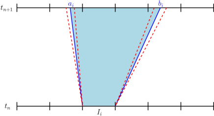
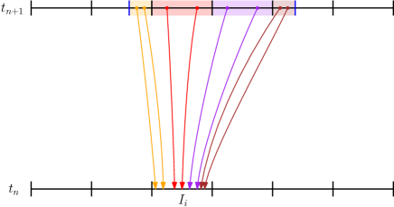
Figure 1: An illustration of the proposed algorithm is shown. First, a forward step (shown on the top) is conducted that determines the domain of influence of the cell $I_{i}$ (the blue lines). Note that as has been pointed out in the text, the true characteristics (dashed red lines) might cross and thus this only yields an approximation. Then in the backward step (shown on the bottom) the region between the two blue lines is divided into parts (illustrated with different colors) each of which overlap with a single cell. In these parts we integrate the characteristics back in time starting at the corresponding Gauss–Legendre quadrature points. The obtained values are then used to update the corresponding degrees of freedom. This backward step is exact up to the error committed in integrating the characteristics.

2.2 Computational complexity

The pseudocode in Algorithm 1 gives us a convenient vehicle to analyze the computational complexity of the present algorithm. In the second loop we iterate over all cells that have a nonempty overlap with the interval $[a_{i},b_{i}]$. In the constant advection case (see, for example, [23, 7, 24, 11, 12, 6, 26, 10]) this implies that we have to consider at most two adjacent cells. However, in the present case the number of cells we have to consider depends on $\tilde{u}^{n}(x_{i+1/2})$ and $\tilde{u}^{n}(x_{i-1/2})$. That is, it depends on how much the magnitude of the solution changes from one cell interface to the next. We note, however, that even for large CFL numbers it is uncommon that more than three cells are processed in that step. Since, except for the first loop (which iterates over the number of cells $n$), the remaining loops only iterate over nodes within a single cell, the numerical algorithms scales as $\mathcal{O}(n)$, i.e. linearly in the number of cells $n$.

Let us also consider what happens as we increase the order $o$ of the numerical scheme. The most computationally intensive part of the algorithm is, by a significant margin, to follow the characteristics backward in time. This function is called $o$ times (once for each quadrature point) and requires a single function evaluation of $u^{n}$ for each iteration of the fixed-point algorithm. Each of these function evaluations scales linearly in the order of the method. Thus, in total the numerical algorithms scales as $\mathcal{O}(o^{2})$. Thus, strictly speaking we do not have linear scaling in the degrees of freedom. However, let us note that on modern computer systems the algorithm (except for extremely large orders) is certainly memory bound. This is further reason for choosing the implementation illustrated in Figure 1 as it facilitates local memory access (both for reading and writing data).

2.3 Improving the fixed-point iteration

As mentioned in the previous section the most compute intensive part of the algorithm is to follow the characteristics backward in time. Thus, decreasing the number of iterations required for the fixed-point iteration would accordingly decrease the time required to run our algorithm. Our goal is still to solve the following fixed-point problem

$$\alpha=x-\tau u^{0}(\alpha).$$

Rewriting this as a root finding problem we obtain

$$f(\alpha)=x-\tau u^{0}(\alpha)-\alpha=0$$

to which we can apply Newton’s method

$$\alpha^{(k+1)}=\alpha^{(k)}+\frac{x-\tau u^{0}(\alpha^{(k)})-\alpha^{(k)}}{1+\tau(u^{0})^{\prime}(\alpha^{(k)})},\qquad\alpha^{(0)}=x.$$

One drawback of this method is that we have to compute $(u^{0})^{\prime}$. Although $(u^{0})^{\prime}$ can be precomputed and consequently the cost is independent of the number of iterations conducted, this is still expensive if only a few iterations are required. In addition, it increases the code complexity significantly. However, the main drawback is that we now require two function evaluations ($u^{0}(\alpha^{(k)})$ and $(u^{0})^{\prime}(\alpha^{(k)})$) per iteration. Nevertheless as we will see in the next section especially for large time steps Newton’s method is clearly superior to performing a fixed-point iteration.

We can, however, remove all of the deficiencies of Newton’s method, while still retaining the speed of convergence, by employing the secant method. In this case we start with a fixed-point iteration

$$\alpha^{(1)}=x-\tau u^{0}(x),\qquad\alpha^{(0)}=x$$

and then continue using the secant method

$$g^{(k)} =x-\tau u^{0}(\alpha^{(k)})-\alpha^{(k)},$$

$$\alpha^{(k+1)} =\alpha^{(k)}-\frac{\left(\alpha^{(k)}-\alpha^{(k-1)}\right)g^{(k)}}{g^{(k)}-g^{(k-1)}}.$$

Within this approach we can reuse the function evaluation from the previous iteration. Moreover, the speed of convergence compared to the fixed-point iteration is greatly improved. We will benchmark these three approaches in section 3.

2.4 Conservation of mass

Both the linear part (3) and the nonlinear part (4) conserve mass. For the latter this can be seen most easily by writing it as a conservation law

$$\partial_{t}u(t,x)+\partial_{x}(\tfrac{1}{2}u^{2}(t,x))=0.$$

This is still true if we replace the exact solution of the linear part by an approximation based on Fourier techniques. Now, let us briefly analyze conservation of mass for the nonlinear part. In previous work for advections that are independent of $u$ (for the case of position dependent advection see [8]; for the case of constant advection see, for example, [23, 7, 24, 13, 11, 12, 6, 26]) mass is preserved by the semi-Lagrangian discontinuous Galerkin scheme. However, this is not true in the present case as the approximation of $u$ is discontinuous at the cell interface. Although that jump is on the order of the discretization error (and thus does not negatively impact accuracy) it implies that either the characteristics cross (resulting in a shock wave) or fan out (resulting in a rarefaction wave). Note that in both cases the solution between the two red dashed lines in Figure 1 can not be (solely) determined by the method of characteristics. Furthermore, the solution is, in general, not smooth across this interface. Since this, in particular, implies that the quadrature is not exact in this region, the numerical scheme described is not mass conservative up to machine precision. It was already pointed out, in a slightly different context, that continuity across the cell interface for the advection speed is necessary in order to obtain a mass conservative semi-Lagrangian discontinuous Galerkin scheme [8].

In principle, this deficiency can be remedied by introducing an additional interval (between the two red dashed lines in Figure 1) on which we use the analytic solution of the Riemann problem to update the numerical solution. This adds additional computational cost but might still be beneficial for problems where, for example, long time integration is essential. We consider this as future work.

Strictly speaking there is one additional error made with respect to mass conservation. Since our scheme is based on the method of characteristics and we therefore do not approximate Burgers’ equation in its conservative form, conservation of mass is only guaranteed if the characteristics are solved exactly. However, in our opinion, this is only a minor issue as the numerical simulations in section 3 demonstrate that using the secant or Newton’s method only a few iterations are sufficient to obtain the characteristics up to machine precision.

3 Numerical simulations

The goal of this section is to both validate the implementation as well as to demonstrate its efficiency for the KP equation. We start in section 3.1 by considering only the nonlinear part of the splitting approach (i.e. Burgers’ equation). Then in section 3.2 we will consider a number of different problems in the context of the KP equation. Finally, in section 3.3 we perform a comparison of the proposed algorithm with the exponential type methods that are considered in [18].

3.1 Burgers’ equation

In this section we evaluate the accuracy and efficiency of the proposed algorithm for the Burgers’ equation by comparing it to a spectral implementation. More specifically, in the latter case we use the fast Fourier transform (FFT) to perform the space discretization and solve the resulting ordinary differential equation using the CVODE library where both the absolute and relative tolerance are set to $10^{-15}$. Of course, if we are only interested in solving Burgers’ equation this would mean that the spectral implementation (which performs many substeps as CVODE implements the fully implicit BDF methods) is orders of magnitude slower compared to our implementation which (as we will see in this section) requires at most a moderate number of iterations. Thus, in this context this is certainly not a sensible comparison. However, for the application we are interested in and which we will consider in the next section, i.e. solving the Kadomtsev–Petviashvili equation, this is still a good indicator of the space discretization error.

Let us start by considering Burgers’ equation on the interval $[0,2\pi]$ using periodic boundary conditions and the initial value

$$u^{0}(x)=\sin x.$$

For the remainder of this section we will refer to this as the sine initial value. The advantage of this choice is that the analytic solution can be expresses as follows

$$u(t,x)=-\sum_{k=0}^{\infty}\frac{2J_{k}(-kt)}{kt}\sin(kx),$$

where $J_{k}(x)$ are the Bessel functions of the first kind. This analytic solution is used to verify our implementation. Let us further remark that the initial value $u(0,x)$ is perfectly smooth but that at $t=1$ the solution develops a discontinuity. Thus, as we increase $t$ we obtain a progressively less regular solution which is more challenging for the higher order methods (including the spectral method).

The numerical results for four different times are shown in Figure 2. We remark that the FFT based approach is generally superior for very regular solutions. However, in all other cases, the eight order discontinuous Galerkin method is on par or superior for the tolerances that are usually of interest in practical applications (i.e. an error at or above $10^{-5}$). We also remark that the less regular the solution becomes the smaller the advantage of the eight order method is compared to the fourth order method. Nevertheless, some advantage with respect to accuracy persists even for $t=0.9$. We have also tried using discontinuous Galerkin methods of order higher than eight. However, those do not result in any additional improvement and we will therefore not consider them further.

In addition, we compare the discontinuous Galerkin method proposed in this paper to Lagrange interpolation of order 4 (as proposed in [13]) and order 6. These results are also shown in Figure 2. We observe that in all configurations considered here the discontinuous Galerkin method outperforms Lagrange interpolation, of the same order, by a significant margin.

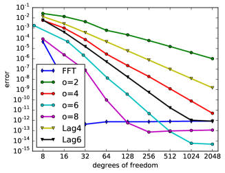
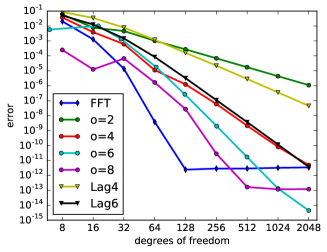
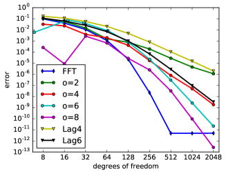
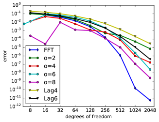
Figure 2: The error in the infinity norm as a function of the degrees of freedom is shown for the sine initial value. From top left to bottom right the error is evaluated at $t=0.1$, $0.5$, $0.8$, $0.9$ corresponding to progressively less regular solutions. For all simulations $10$ iterations with the secant method are conducted and the numerical solution is compared to the analytic solution in order to determine the error.

As a second example, we will consider Burgers’ equation on the interval $[-L,L]$ with periodic boundary conditions and the initial value

$$u^{0}(x)=\text{sech}\,x=\frac{1}{\text{cosh}\,z}.$$

For the remainder of this section we will refer to this as the sech initial value. Choosing this initial value is motivated by the fact that in many applications of the KP equation we consider initial values that decay to zero as $x\to\infty$ but are not exactly periodic on the truncated domain that we have to employ in a numerical simulation. This then usually means that we have to choose $L$ relatively large in order to render errors due to the truncation of the physical domain negligible.

In Figure 3 we investigate the performance of the discontinuous Galerkin approach as a function of regularity (i.e. as a function of the final time). We observe that the FFT implementation is, in general, superior to the discontinuous Galerkin approach. However, the difference in the number of degrees of freedom needed, for a given accuracy, for the 8th order discontinuous Galerkin method is always less than a factor of two. The discontinuous Galerkin approach outperforms Lagrange interpolation (except at tolerances below $10^{-2}$ and $t=0.2$).

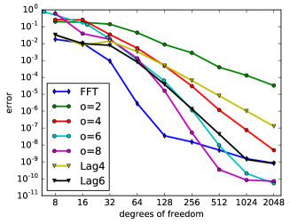
Figure 3: The error in the infinity norm as a function of the degrees of freedom is shown for the sech initial value. We consider a final time $t=0.2$ (left) and $t=1.1$ (right). In both cases the domain is truncated at $L=20$. For all simulations $10$ iterations with the secant method are conducted. The error is computed by comparing the numerical solution with a FFT based reference solution that uses $8192$ degrees of freedom.

As the third and final example we consider Burgers’ equation on the interval $[-1,1]$ with periodic boundary conditions and initial value

$$u^{0}(x)=\cos\left(\omega(\tfrac{1}{2}+|x|)x\right)\Psi(x)$$

with the bump function $\Psi(x)=\exp(-1/(1-x^{2}))$ and $\omega=20$. For the remainder of this section we will refer to this as the oscillating initial value. Once again we investigate the accuracy of the discontinuous Galerkin and FFT implementation as a function of the regularity of the solution. The corresponding numerical results are shown in Figure 4. As the regularity decreases the relative performance of the eight order discontinuous Galerkin scheme, compared to the FFT implementation, increases. For the configuration with $t=0.1$ the performance of these two methods is almost identical. As before, we observe that the discontinuous Galerkin method outperforms Lagrange interpolation by a significant margin.

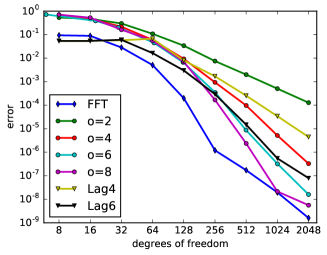
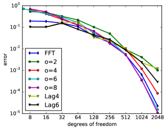
Figure 4: The error at $t=0.05$ (left) and $t=0.1$ (right) as a function of the degrees of freedom is shown for the oscillating initial value. For all simulations $10$ iterations with the secant method are conducted. The error is computed by comparing the numerical solution with a FFT based reference solution that uses $8192$ degrees of freedom.

The issue of domain truncation (as considered for the sech initial value) is particularly important for the KP (and other dispersive) equation and it thus deserves some additional comments. While we have shown here that the discontinuous Galerkin method can be very competitive compared to the FFT based implementation, this is certainly not the end of the story for this particular method. What can be done relatively easily for the discontinuous Galerkin method is to employ a grid where not all cells have the same size. Therefore, in the spirit of a block-structured mesh refinement scheme we would keep the present resolution in the center of the domain (where the majority of the dynamics happens) and use larger cells (with possible lower order) in the part of the domain where the solution is small. This would significantly reduce the computational effort with almost no loss in accuracy. Such an optimization is very difficult to do within the FFT framework and would thus further work in favor of the numerical scheme proposed in this paper. We consider this as future work.

To conclude this section, let us investigate how many iterations are required in order to obtain an accurate solution. For that purpose we consider the three methods described in section 2.3 (fixed-point iteration, secant method, and Newton’s method) and solve Burgers’ equation using the sine initial value. The numerical results are shown in Figure 5. We observe that, while the fixed-point iteration can converge slowly if we take excessively large time steps, for the secant method and Newton’s method no more than a couple of iterations are necessary. In fact, for these methods the number of iterations required to reach a certain precision is only weakly dependent on the time step size. Let us note that the secant method requires the same computational effort compared to fixed-point iteration while Newton’s method (which requires the construction of the derivative) is approximately twice as costly. Thus, in order to minimize the computational effort for a given accuracy we have chosen to exclusively use the secant method in the examples that are presented in the next section.

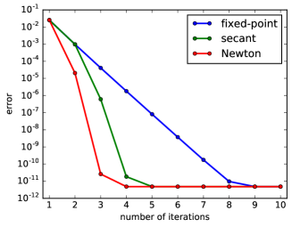
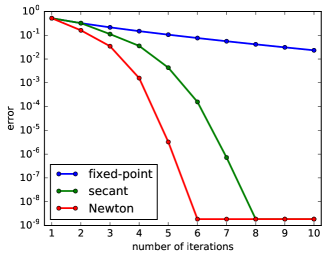
Figure 5: Error in the infinity norm as a function of the number of iterations is shown for the sine initial value at $t=0.05$ (left) and $t=0.8$ (right). The space discretization uses the fourth order method ($o=4$) with $512$ cells and the numerical solution is compared to the analytic solution in order to obtain the error.

3.2 Kadomtsev–Petviashvili equation

First let us consider numerical results for the KP I and KP II equations using the Schwartzian initial value

$$u(0,x,y)=-\partial_{x}\text{sech}^{2}\left(\sqrt{x^{2}+y^{2}}\right).$$

In all simulations we have chosen $\epsilon=0.1$ and use the computational domain $[-10\pi,10\pi]\times[-10\pi,10\pi]$. This is precisely the initial value that has been used in [18]. If not indicated otherwise we always use $5$ iterations with the secant method to determine the characteristic curves required in our algorithm.

First, let us consider the KP II equation (i.e. $\lambda=1$). The numerical results for final time $t=0.4$ are shown in Figure 6. This solution agrees very well with what has been reported in the literature (see, for example, [19]). In addition, we investigate the error as the number of degrees of freedom is increased as well as the error as we decrease the time step size (all errors are computed in the infinity norm and are compared to a reference solution with a sufficiently fine resolution). We find that for low to medium precision requirements the fifth and seventh order discontinuous Galerkin method yields the best performance, respectively.

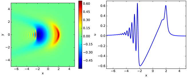
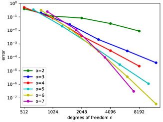
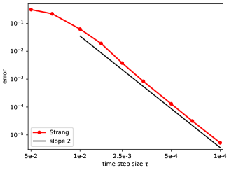
Figure 6: The numerical simulation for the KP II equation using the Schwartzian initial value is shown at $t=0.4$ for the two-dimensional domain (top-left) and for a one-dimensional slice with $y=0$ (top-right). The fourth order method (for Burgers’ equation) with a time step size of $\tau=10^{-3}$ has been used. In addition, the error for the discontinuous Galerkin methods is shown as a function of the degrees of freedom (bottom-left) and the error as a function of the time step size $\tau$ is shown (bottom-right). For the former the error is determined by comparing the numerical approximation to a reference solution with $o=7$ and $28672$ degrees of freedom in the $x$-direction, while for the latter a reference solution with time step size $\tau=5\cdot 10^{-5}$ is used.

Before proceeding, let us discuss the number of iterations $i$ required in the nonlinear solver. For the secant method it is generally sufficient to perform $i=3$ iterations. The same level of precision is achieved for the fixed-point iteration for $i=5$ iterations. We note that the advantage of the secant method increases significantly for more stringent tolerances. Thus, we conclude that while the relative difference is not as large as in the numerical simulations conducted in section 3.1 (due to the fact that the splitting error limits the time step size for a given accuracy), we can still obtain a significant saving in computational resources by employing the secant method.

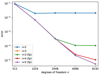
Figure 7: The error is shown as a function of the degrees of freedom for various numbers of iterations $i$ for the fixed-point (fp) and the secant method (note that the lines for the secant method with $i=3$ and the fixed-point iteration with $i=5$ are indistinguishable in the plot). The error is determined by comparing the numerical approximation to a reference solution with $i=20$ iteration using the secant method.

Second, we turn our attention to the KP I model (i.e. $\lambda=-1$). The numerical results for final time $t=0.4$ are shown in Figure 8. Once again we remark that these results agree very well with what has been reported in the literature. We find that for low to medium precision requirements the fourth and seventh order discontinuous Galerkin method yields the best performance, respectively.

For the KP equation the mass is an invariant. However, the discontinuous Galerkin method used to solve Burgers’ equation does not conserve mass exactly (see section 2.4). The error in mass is shown in Figure 8, where the problem is set up such that all numerical methods use $2048$ degrees of freedom in the $x$-direction. For the fourth, fifth, sixth, and seventh order method this corresponds to an error in the infinity norm of approximately $10^{-2}$. The error in mass for these methods, however, is on the order of $10^{-6}$. Thus, even though the proposed numerical method does not conserve mass exactly, the error is very small.

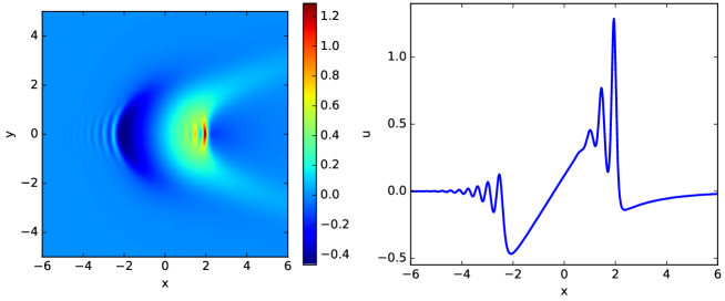
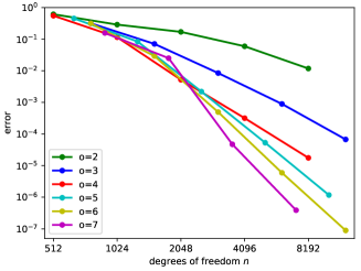
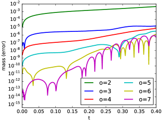
Figure 8: The numerical simulation for the KP I equation using the Schwartzian initial value is shown at $t=0.4$ for the two-dimensional domain (top-left) and for a one-dimensional slice with $y=0$ (top-right). The fourth order method with a time step size of $\tau=10^{-3}$ has been used. In addition, the error for the discontinuous Galerkin methods is shown as a function of the degrees of freedom (bottom-left). The error is determined by comparing the numerical approximation to a reference solution with $o=7$ and $28672$ degrees of freedom in the $x$-direction. The error in mass is shown as a function of time (bottom-right). In the latter all configurations use $2048$ degrees of freedom in the $x$-direction.

Next, let us consider the soliton solution

$$u(t,x,y)=c\,\text{sech}^{2}(a(x-bt)),$$ (14)

where $c=2$, $a=\epsilon\sqrt{c/2}$, and $b=2c\epsilon^{2}$. This solution maintains the same shape in space as time goes on and we will thus use it to test the long time behavior of our numerical method. In the following simulation, we impose $u(0,x,y)$ as the initial condition for the KP I equation with $\epsilon=1$. The soliton given by equation (14) is only an exact solution on the entire plane. In order to reproduce this situation as closely as possible we will use a sufficiently large computational domain with periodic boundary conditions.

For the present test we integrate the KP equation until time $t=500$. For each of the methods we employ $512$ degrees of freedom in the $x$-direction and a time step size $\tau=10^{-2}$ (which means that we perform a total of $5\cdot 10^{4}$ time steps). A slice of the solution (for $y=0$) at time $t=500$ is shown in Figure 9. We remark that no spurious oscillations are visible even for the higher order methods.

It should be duly noted that in this case our numerical method operates far away from the asymptotic regime (this is true for both the time integration and the space discretization). The described behavior is also apparent from Figure 9 as the predicted speed of advection (i.e. how far the numerical solution travels in a given time span) does not match that of the exact solution. As a consequence, the error in the infinity norm is large.

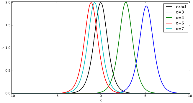
Figure 9: The slice $x\mapsto u(500,x,0)$ of the numerical approximation to equation (14) is shown. All numerical methods employ $512$ degrees of freedom in the $x$-direction and a time step size of $\tau=10^{-2}$ has been used. The exact solution can be computed analytically and at $t=500$ is identical to the initial value.

Nevertheless, the proposed numerical methods (in particular, the higher order variants) still show good qualitative agreement with the exact solution. For example, the amplitude and the shape of the soliton matches that of the exact solution very well. Thus, we will consider here how well the numerical method preserves certain qualitative features of the exact solution.

More specifically, the figure of merit we are looking at here is how well the amplitude (i.e. the maximum) and the mass of the soliton is preserved. The corresponding results are shown in Figure 10. We observe that employing higher order methods yields a significant decrease in the error of both quantities. In particular, we see a drastic improvement going from second to third, from third to fourth, and from fourth to fifth order, while keeping the degrees of freedom and thus (at least approximately) the computational cost the same.

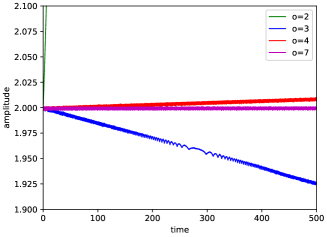
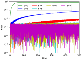
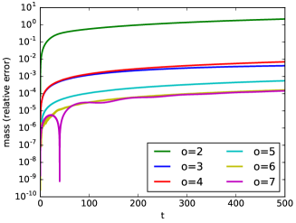
Figure 10: The amplitude of the numerical approximation to the soliton solution (see equation (14)) is shown as a function of time (top-left). In addition, the error in amplitude is plotted on a logarithmic scale (top-right). At the bottom, the relative error in mass is shown as a function of time. All numerical methods employ $512$ degrees of freedom in the $x$-direction and a time step size of $\tau=10^{-2}$ has been used.

3.3 Performance comparison

In this section we will compare the performance of the proposed numerical method to an approach based on exponential integrators. Exponential integrators were evaluated for this problem in [18] where they were shown to perform best compared to a range of numerical methods (in particular, fully implicit methods and IMEX schemes). The seductive property of these methods is that the space discretization can be done completely with FFTs. Assuming a smooth solution this implies superpolynomial convergence. Their disadvantage is that they treat the nonlinearity explicitly and that (for the same number of degrees of freedom) they are significantly more expensive compared to the splitting approach (see [13]).

Due to the significant difference between these two methods it is very difficult to obtain a meaningful comparison by simply looking at the run time of the two implementations we use in this paper. This is in part due to the fact that in both implementations much room is left for further optimizations (mainly from a computer science perspective). Furthermore, we have spent significantly more time optimizing the splitting/discontinuous Galerkin method compared to the exponential integrator based approach. In order to enable a meaningful comparison, we will now develop a model that gives us a good idea of how expensive these two algorithms are on a modern computer system.

Let us start with the splitting approach. In this case we will use an equidistant grid in the $y$-direction in order to facilitate the FFT that needs to be computed. However, for the $x$-direction we will use an equidistant grid for the linear part (where we have to take FFTs) and the discontinuous Galerkin approximation for the nonlinear part. The former will have $n_{x}n_{y}$ degrees of freedom, while for the latter we use $N_{x}n_{y}$ degrees of freedom (reflecting the fact that we might need more grid points to achieve the same accuracy for the dG method as compared to the FFT approach). We also need a method to transfer the results of the dG computation back to the equidistant grid (an interpolation procedure).

In addition, the splitting (as well as the exponential integrator) approach requires us to compute the action of the matrix exponential $\mathrm{e}^{\tau A}u$. This is done in Fourier space and requires the multiplication with a factor that depends on the step size $\tau$ and on the frequency. Since this factor involves an exponential, it is rather expensive to compute. However, we can precompute these quantities and store the result in an array. Before proceeding let us note that this situation is, in principle, the same for the exponential integrator. However, in the latter case more matrix functions are required, which increases the storage cost somewhat, and care has to be taken when evaluating the $\varphi_{k}$ functions in order to avoid large round off errors.

Our computational model will assume that all involved operations (FFT, interpolation, semi-Lagrangian discontinuous Galerkin scheme, array addition and multiplication) are memory bound. That is, the performance is dictated by how much data can be transferred to and from memory (and not by how many arithmetic operations have to be performed). This is a reasonable assumption on all modern computer systems. We should note, however, that achieving this level of performance requires an optimized implementation. In a sense this can be considered as a (realistic) best case for both algorithms.

Using this assumption we can count the number of memory accesses per time step that are required for the splitting/discontinuous Galerkin scheme. The results are shown in Table 1.

	number	memory accesses	total memory accesses
FFT	$2$	$2n_{x}n_{y}$	$4n_{x}n_{y}$
$\mathrm{e}^{\tau A}$	$1$	$3n_{x}n_{y}$	$3n_{x}n_{y}$
Interpolation	$1$	$2N_{x}n_{y}$	$2N_{x}n_{y}$
dG	$1$	$N_{x}n_{y}$	$N_{x}n_{y}$
Strang splitting			$(7n_{x}+3N_{x})n_{y}$

Table 1: The number of memory accesses required for one time step of the second order Strang splitting/discontinuous Galerkin scheme are listed. The number of grid points in the $y$-direction is denoted by $n_{y}$. The number of grid points in the $x$-direction is denoted by $n_{x}$/$N_{x}$ for the equidistant/dG grid.

Now, let us turn our attention to the exponential integrator of order $2$ which can be written as

$$U =\mathrm{e}^{\tau A}u^{n}+\tau\varphi_{1}(\tau A)B(u^{n})$$

$$u^{n+1} =U+\tau\varphi_{2}(\tau A)(B(U)-B(u^{n}))$$

or for our specific problem

$$U =\mathrm{e}^{\tau A}u^{n}-6\tau\varphi_{1}(\tau A)(u_{x}^{n}u^{n})$$

$$u^{n+1} =U-6\tau\varphi_{2}(\tau A)(UU_{x}-u_{x}^{n}u^{n}).$$

In the following we will refer to this method as exp2. It is seductive to just count how many FFTs, additions, etc., one has to compute but this would give an overestimation of the true computational cost (as certain operations can be combined which due to caching will reduce the number of memory transactions). For our performance analysis we will consider the implementation given in Table 2.

step	computation	mem acc	remark
1.	$\hat{u}^{n}=\mathcal{F}(u^{n})$	$0$	available from previous step
2.	$u_{x}^{n}=\mathcal{F}^{-1}(ik\hat{u}^{n})$	$4n_{x}n_{y}$
3.	$B=u_{x}^{n}\cdot u^{n}$	$3n_{x}n_{y}$
4.	$\hat{B}=\mathcal{F}(B)$	$2n_{x}n_{y}$
5.	$\hat{U}=\Phi_{0}\cdot\hat{u}^{n}+\Phi_{1}\cdot\hat{B}$	$5n_{x}n_{y}$
6.	$U=\mathcal{F}^{-1}(\hat{U})$	$2n_{x}n_{y}$
7.	$U_{x}=\mathcal{F}^{-1}(ik\hat{U})$	$4n_{x}n_{y}$
8.	$F=U\cdot U_{x}-B$	$4n_{x}n_{y}$
9.	$\hat{F}=\mathcal{F}(F)$	$2n_{x}n_{y}$
10.	$\hat{u}^{n+1}=\hat{U}+\Phi_{2}\cdot\hat{F}$	$4n_{x}n_{y}$
11.	$u^{n+1}=\mathcal{F}^{-1}(\hat{u}^{n+1})$	$2n_{x}n_{y}$
Total cost		$32n_{x}n_{y}$

Table 2: The different steps required for the second order exponential integrator are listed together with the number of memory accesses (mem acc). Note that $\mathcal{F}$ and $\mathcal{F}^{-1}$ denote the FFT and inverse FFT, respectively. The arrays $\Phi_{0},\Phi_{1},\Phi_{2}$ contain the precomputed factors required to apply the various matrix functions in Fourier space.

It is clear that the Strang splitting scheme has a decisive advantage for $N_{x}=n_{x}$ (as has already been pointed out in [13]). However, since the approximation error made by the Fourier transform converges superpolynomially this is often not a very realistic assumption. Furthermore, this does not take into account the difference in accuracy between the splitting method and the exponential integrator. In order to compare the two numerical methods on an equal footing we consider for both methods a range of tolerances. At these tolerances we balance the time and space discretization error (by choosing an appropriate time step size and the number of degrees of freedom) and then determine the computational cost according to the model described here. The corresponding results for the KP equation with the Schwartzian initial value (using precisely the setup from section 3.2) are shown in Figure 11.

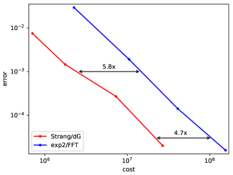
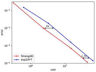
Figure 11: The error for the Strang splitting/discontinuous Galerkin ($o=5$) and the exp2 scheme as a function of the computational cost is shown for the KP I equation (left) and the KP II equation (right) using the Schwartzian initial value (the setup from section 3.2 is employed). The computational cost is in arbitrary units and is determined according to the model described in this section.

We can clearly see that the Strang splitting/discontinuous Galerkin scheme is superior for the small to medium accuracy requirements that are often important in practice. For tighter tolerances the exp scheme eventually becomes the method of choice (since the faster convergence of the Fourier transform eventually overcomes the disadvantage of the time integrator).

4 Conclusion & Outlook

In this paper we have proposed an arbitrary order (in space) numerical method to solve the Kadomtsev–Petviashvili equation based on time splitting. In particular, treating the nonlinearity with a semi-Lagrangian discontinuous Galerkin approach results in an unconditionally stable scheme. We have demonstrated the efficiency of this numerical method by providing a range of numerical examples. In particular, we have compared our approach to an exponential integrator (which has the advantage that the entire space discretization can be done using spectral methods) and observe superior performance for small to medium accuracy requirements (arguably the regime most important in applications).

Although we have exclusively focused on the KP equation in this paper, the proposed method can conceivably be extended to any partial differential equation which combines a stiff linear part with a Burgers’ type nonlinearity. To name just a few that are of interest in the sciences: the Kawahara equation, the (deterministic or stochastic) Kardar–Parisi–Zhang equation, the viscous Burgers’ equation (in particular its multi-dimensional generalizations [15]), the Korteweg–de Vries equation, and even the Navier–Stokes equation. In some sense the KP equation is more difficult than some of these other models as no diffusion is included (the KP equation is a purely hyperbolic system).

We also consider this work as a first step towards efficiently solving the KP equation (and other partial differential equations with higher order derivatives) on a non-tensor-product grid. In this case the dispersive part can not be solved using fast Fourier techniques (as is done in this paper). Nevertheless, within the splitting approach introduced, a preconditioned implicit method for the linear dispersion can be combined with our semi-Lagrangian discontinuous Galerkin method to solve Burgers’ equation. We consider this as future work.

References

- [1] M.J. Ablowitz and H. Segur. On the evolution of packets of water waves. J. Fluid Mech., 92(04):691–715, 1979.
- [2] O. Bokanowski, Y. Cheng, and C. Shu. Convergence of discontinuous Galerkin schemes for front propagation with obstacles. Math. Comput., 85(301):2131–2159, 2016.
- [3] O. Bokanowski and G. Simarmata. Semi-Lagrangian discontinuous Galerkin schemes for some first- and second-order partial differential equations. ESAIM: Math. Model. Numer. Anal., 50(6):1699–1730, 2016.
- [4] X. Cai, W. Guo, and J. Qiu. A high order conservative semi-Lagrangian discontinuous Galerkin method for two-dimensional transport simulations. J. Sci. Comput., 73(2):514–542, 2017.
- [5] R.M. Chen. Some nonlinear dispersive waves arising in compressible hyperelastic plates. Int. J. Eng. Sci., 44(18–19):1188–204, 2006.
- [6] N. Crouseilles, L. Einkemmer, and E. Faou. An asymptotic preserving scheme for the relativistic Vlasov–Maxwell equations in the classical limit. Comput. Phys. Commun., 209:13–26, 2016.
- [7] N. Crouseilles, M. Mehrenberger, and F. Vecil. Discontinuous Galerkin semi-Lagrangian method for Vlasov–Poisson. In ESAIM: Proceedings, volume 32, pages 211–230. EDP Sciences, 2011.
- [8] N. Crouseilles, M. Mehrenberger, and F. Vecil. A Discontinuous Galerkin semi-Lagrangian solver for the guiding-center problem. HAL preprint, hal–00717155, 2012.
- [9] E. Demler and A. Maltsev. Semiclassical solitons in strongly correlated systems of ultracold bosonic atoms in optical lattices. Ann. Phys., 326(7):1775–1805, 2011.
- [10] L. Einkemmer. High performance computing aspects of a dimension independent semi-Lagrangian discontinuous Galerkin code. Comput. Phys. Commun., 202:326–336, 2016.
- [11] L. Einkemmer. On the geometric properties of the semi-Lagrangian discontinuous Galerkin scheme for the Vlasov–Poisson equation. arXiv preprint, arXiv:1601.02280, 2016.
- [12] L. Einkemmer and A. Ostermann. Convergence analysis of a discontinuous Galerkin/Strang splitting approximation for the Vlasov–Poisson equations. SIAM J. Numer. Anal., 52(2):757–778, 2014.
- [13] L. Einkemmer and A. Ostermann. A splitting approach for the Kadomtsev–Petviashvili equation. J. Comput. Phys., 299:716–730, 2015.
- [14] F. Filbet and E. Sonnendrücker. Comparison of Eulerian Vlasov solvers. Comput. Phys. Commun., 150(3):247–266, 2003.
- [15] U. Frisch and J. Bec. Burgulence. In M. Lesieur, A. Yaglom, and F. David, editors, New trends in turbulence. Turbulence: nouveaux aspects. Les Houches - Ecole d’Ete de Physique Theorique, volume 74. Springer, Berlin, Heidelberg, 2001.
- [16] W. Guo, R.D. Nair, and J. Qiu. A conservative semi-Lagrangian discontinuous Galerkin scheme on the cubed sphere. Mon. Weather Rev., 142(1):457–475, 2014.
- [17] B.B. Kadomtsev and V.I. Petviashvili. On the stability of solitary waves in weakly dispersing media. Sov. Phys. Dokl., 15:539–541, 1970.
- [18] C. Klein and K. Roidot. Fourth order time-stepping for Kadomtsev–Petviashvili and Davey–Stewartson equations. SIAM J. Sci. Comput., 33(6):3333–3356, 2011.
- [19] C. Klein and J.C. Saut. Numerical study of blow up and stability of solutions of generalized Kadomtsev–Petviashvili equations. J. Nonlinear Sci., 22(5):763–811, 2012.
- [20] C. Klein, C. Sparber, and P. Markowich. Numerical study of oscillatory regimes in the Kadomtsev–Petviashvili equation. J. Nonlinear Sci., 17(5):429–470, 2007.
- [21] A.A. Minzoni and N.F. Smyth. Evolution of lump solutions for the KP equation. Wave Motion, 24(3):291–305, 1996.
- [22] Y. Ohno and Z. Yoshida. Nonlinear ion acoustic waves scattered by vortexes. Commun. Nonlinear Sci., 38:277–287, 2016.
- [23] J.M. Qiu and C.W. Shu. Positivity preserving semi-Lagrangian discontinuous Galerkin formulation: theoretical analysis and application to the Vlasov–Poisson system. J. Comput. Phys., 230(23):8386–8409, 2011.
- [24] J.A. Rossmanith and D.C. Seal. A positivity-preserving high-order semi-Lagrangian discontinuous Galerkin scheme for the Vlasov–Poisson equations. J. Comput. Phys., 230(16):6203–6232, 2011.
- [25] E. Sonnendrücker, R. Jean, P. Bertrand, and A. Ghizzo. The semi-Lagrangian method for the numerical resolution of the Vlasov equation. J. Comput. Phys., 149(2):201–220, 1999.
- [26] C. Steiner, M. Mehrenberger, and D. Bouche. A semi-Lagrangian discontinuous Galerkin convergence. HAL preprint, hal–00852411, 2013.
- [27] E. Zauderer. Partial differential equations of applied mathematics. John Wiley & Sons, 2011.