X-ray and gamma-ray emission from middle-aged supernova remnants in cavities: 1. Spherical symmetry

Abstract

We present analytical and numerical studies of models of supernova-remnant (SNR) blast waves expanding into uniform media and interacting with a denser cavity wall, in one spatial dimension. We predict the nonthermal emission from such blast waves: synchrotron emission at radio and X-ray energies, and bremsstrahlung, inverse-Compton emission (from cosmic-microwave-background seed photons; ICCMB), and emission from the decay of $\pi^{0}$ mesons produced in inelastic collisions between accelerated ions and thermal gas, at GeV and TeV energies. Accelerated particle spectra are assumed to be power-laws with exponential cutoffs at energies limited by the remnant age or (for electrons, if lower) by radiative losses. We compare the results with those from homogeneous (“one-zone”) models. Such models give fair representations of the 1-D results for uniform media, but cavity-wall interactions produce effects for which one-zone models are inadequate. We study the time evolution of SNR morphology and emission with time. Strong morphological differences exist between ICCMB and $\pi^{0}$-decay emission; at some stages, the TeV emission can be dominated by the former and the GeV by the latter, resulting in strong energy-dependence of morphology. Integrated gamma-ray spectra show apparent power-laws of slopes that vary with time, but do not indicate the energy distribution of a single population of particles. As observational capabilities at GeV and TeV energies improve, spatial inhomogeneity in SNRs will need to be accounted for.

1. Introduction

Supernova remnants, along with pulsar-wind nebulae, are the most obvious examples of Galactic fast-particle production. GeV electrons have been known to be present since the widespread adoption of Shklovsky’s 1953 suggestion of synchrotron emission as the process producing radio emission from SNRs (Shklovsky 1953). The range of observable electron energies was extended to the TeV range with the discovery of X-ray synchrotron emission from SN 1006 (Reynolds & Chevalier 1981; Koyama et al. 1995). A dozen or so Galactic shell supernova remnants (SNRs) now show evidence for X-ray synchrotron emission at least in localized areas. See Reynolds (2008), R08, for a review.

The advent of GeV/TeV astronomy has made possible the more detailed characterization of relativistic-particle populations in SNRs. Of the remnants showing X-ray synchrotron emission, TeV emission with a shell morphology is observed from G347.3-0.5 (RX J1713.7-3946), SN 1006, RCW 86, G266.2-1.2 (“Vela Jr.”), and HESS J1731-347 (see Rieger et al. (2013) for a review), along with unresolved or complex emission from Cassiopeia A and Tycho (Acciari et al. 2010; Giordano et al. 2012). This emission could be due to leptonic processes (bremsstrahlung or inverse-Compton [IC] emission) or hadronic processes (inelastic pp scattering producing pions, of which $\pi^{0}$’s decay to photons) (see R08 for a review). Firm evidence for hadronic emission would demonstrate directly that SNRs produce cosmic-ray ions, and would be an important advance. While various authors (e.g., Morlino & Caprioli 2012; Berezhko & Völk 2008) suggest that this is the case in several of the above objects, the one-zone models typically used are sufficiently oversimplified that there is still room for debate (e.g., Atoyan & Dermer (2012) for Tycho). The Fermi LAT instrument has added considerably to the observational constraints that models must meet; GeV observations of G347.3-0.5 (Abdo et al. 2011) appear to disfavor hadronic models (e.g., Ellison et al. 2012), while those of Cas A can support a hybrid model involving both mechanisms (e.g., Araya & Cui 2010).

Fermi has also demonstrated the existence of a largely unanticipated class of SNR sources, older objects interacting with molecular clouds (e.g., Abdo et al. 2010). In these cases, X-ray synchrotron emission is absent, as the shock waves are currently too slow to accelerate electrons to the required TeV energies. However, GeV protons can easily produce GeV photons through the $\pi^{0}$ process, and these objects have been successfully modeled this way (e.g., IC 443 and W44 Ackermann et al. 2013). Even here, though, it is not absolutely clear if newly accelerated protons are necessary; simple compression of ambient cosmic-ray protons may be sufficient (Uchiyama et al. 2010).

A potential third class of Fermi SNR sources may exist: middle-aged ($t\mathrel{\mathchoice{\lower 3.1pt\vbox{\halign{$\m@th\displaystyle\hfil#\hfil$\cr>\crcr\sim\crcr}}}{\lower 3.1pt\vbox{\halign{$\m@th\textstyle\hfil#\hfil$\cr>\crcr\sim\crcr}}}{\lower 3.1pt\vbox{\halign{$\m@th\scriptstyle\hfil#\hfil$\cr>\crcr\sim\crcr}}}{\lower 3.1pt\vbox{\halign{$\m@th\scriptscriptstyle\hfil#\hfil$\cr>\crcr\sim\crcr}}}}2000$ yr) SNRs which are interacting with low-density media (e.g., Pup A; Hewitt et al. 2012). The Cygnus Loop (Fig. 1) could belong to this class. Here the ambient or internal gas densities may not be sufficient for a hadronic explanation, especially since the Cygnus Loop appears to have resulted from an explosion in a wind-blown cavity. In this paper we explore the GeV/TeV emission to be expected from a SNR exploding in a low-density cavity, subsequently interacting with the cavity wall.

Cavity explosions have been the subject of theoretical investigation for many years. Early 1-D numerical hydrodynamic studies were done by Tenorio-Tagle et al. (1990, 1991) focusing on realistic stellar-wind environments, and on SNRs that had reached the radiative phase. These studies predicted optical and thermal X-ray emission from such interactions. Dwarkadas (2005) examined this problem, focusing on earlier stages of evolution, and on thermal X-ray emission.

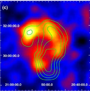
Figure 1.— Fermi image of the Cygnus Loop, with radio contours (Katagiri et al. 2011).

Simulations of the interaction of a fast Wolf-Rayet (WR) wind with a slower, previous red supergiant (RSG) wind show that the shocked fast wind can occupy the bulk of the cavity volume, with material of roughly constant density, bounded by a thin shell with very much higher density (van Marle & Keppens 2012). Such cavities can be as large as 10 pc or greater (van Marle et al. 2015). Since we are interested in later stages of SNR evolution in which any unshocked stellar wind has already been swept up, and for which the SNR blast wave is in the Sedov phase, we shall assume that the remaining cavity with which the blast wave interacts has constant density. We shall also assume that the shell bounding the cavity is sufficiently thick that the blast wave has not emerged by the time our simulations end. Unlike most previous studies, we focus on nonthermal emission, in particular that produced just before and for some time after the interaction.

A few calculations of SNR evolution have been published using numerical hydrodynamics coupled with realistic shock-acceleration physics, predicting both thermal and nonthermal emission (e.g., Lee et al. 2013). However, such models are computationally expensive and have been reported for only a few cases. Most GeV/TeV modeling of SNRs has been done in a “one-zone” (or zero-dimensional) context: a spatially homogeneous source (although often with considerable sophistication in the spectral modeling , e.g., Abdo et al. (2009) among many others). An important question is the extent to which such modeling reflects realistic sources. Here we begin an investigation of this question with a suite of spherically symmetric (1-D) models of cavity explosions. These models are compared with one-zone and analytic models, and with 1-D models of expansion into a uniform medium. A larger range of models, with parameter studies, is given in Tang (2016; PhD thesis, in preparation).

2. Dynamics, Particle Acceleration, and Magnetic-Field Evolution

We consider two cases: evolution in a uniform medium, and evolution in a cavity of uniform density ($n_{0}=0.25$ cm^-3) bounded by a wall (at $R=2.67\times 10^{19}$ cm) of much higher but still uniform density (20 times higher). In the uniform case, we assume all ejecta have been reheated by the reverse shock, corresponding to the Sedov self-similar solution. In the cavity case, the interaction of the blast wave with the cavity wall drastically slows the blast wave while creating a reflected shock wave that moves back toward the remnant center. In one dimension, the reflected shock is eventually reflected back out and returns to the blast wave. However, we do not include cooling in our simulations, so we consider only shock velocities above about 300 km s^-1 (see below), and for the parameter ranges we consider, by the time the blast wave speed has dropped to this value, the reflected shock has not reached the center yet. We treat the uniform case both analytically and numerically; the cavity case is treated numerically only. We use the versatile grid-based hydrodynamics code VH-1, a conservative, finite-volume code for solving the equations of ideal hydrodynamics, based on the Lagrangian remap version of the Piecewise Parabolic Method (Colella & Woodward 1984). The code is third order in space and second order in time. We assume that the blast wave dynamics are not affected by cosmic-ray pressure (the low-efficiency limit). The grid of 1000 linearly spaced radial zones expands to follow the moving blast wave.

We neglect cooling in these simulation. Blondin et al. (1998) give the characteristic time for the cooling transition for a blast wave in a uniform medium as

$$t_{\rm tr}=2.9\times 10^{4}\,E_{51}^{4/17}\,n_{0}^{-9/17}\ {\rm yr}$$ (1)

where $E_{51}$ is the explosion energy in units of $10^{51}$ erg, and $n_{0}$ is the upstream number density (assuming cosmic abundances). At this time, the blast-wave velocity is

$$v_{\rm shock}(t_{\rm tr})=260\,E_{51}^{1/17}\,n_{0}^{2/17}.$$ (2)

We use the second criterion, since for a cavity explosion, the blast wave will reach the cavity wall rapidly, then decelerate fairly quickly. The material in the cavity will have a much longer cooling time. We follow our simulations to blast-wave speeds of about 320 km s^-1, slightly higher than $v_{\rm shock}(t_{\rm tr})\sim 310$ km s^-1 for an upstream density $n_{0}=5$ cm^-3 and $E_{51}=1$.

2.1. Particle acceleration

Relativistic particles are assumed accelerated at the shock front to a maximum energy limited by either the finite remnant age or (for electrons) radiative losses, if that limitation is more restrictive. A constant fraction $\zeta=10^{-4}$ of ions with momentum above some value (here taken to be ten times the thermal proton momentum $m_{p}v_{\rm shock}$) is assumed to be accelerated, with a power-law distribution of specified slope. The same spectrum of electrons, with a normalization lower by a factor $k_{ei}=0.02$, is assumed to be produced. (These values are typical of shock-acceleration models; see, e.g., Lee et al. (2013)). Maximum energies are calculated for each fluid element, and the particle population then evolves by adiabatic (and for electrons, synchrotron) losses. Diffusion is neglected. This treatment of the particle populations is similar to that used in Reynolds (1998), R98, differing slightly only in now normalizing the accelerated-particle distributions by $\zeta$ and $k_{ei}$.

We consider accelerated ions to have a simple power-law momentum distribution, $N_{i}({\bf p})=K_{p}{\bf p}^{-\sigma}$. In standard test-particle DSA, $\sigma=3r/(r-1)$ where $r$ is the shock compression ratio. Then for the magnitude of momentum, $N_{i}(p)dp=(4\pi p^{2}dp)N_{i}({\bf p})dp=4\pi K_{p}\,p^{2-\sigma}\,dp$. Then the energy distribution is

$$N_{i}(E)=N_{i}(p){dp\over dE}\equiv K_{i}E^{-b}\ \Rightarrow\ K_{i}=4\pi K_{p}\,{dp\over dE}\,p^{2-\sigma}\,E^{b}.$$ (3)

The index $b$ will take on different values in the nonrelativistic (NR) and extreme-relativistic (ER) regimes, because of the different dependence of $p(E)$. We approximate the distribution as two straight power-laws with energy indices $q$ and $s$, respectively, joined at $m_{p}c^{2}$. For the NR regime, $dp/dE=\sqrt{m/2E}$ and

$$K_{i}({\rm NR})=4\pi K_{p}\,m^{(3-\sigma)/2}\,2^{(1-\sigma)/2}\,E^{s+(1-\sigma)/2}\ \Rightarrow\ q=(\sigma-1)/2$$ (4)

in order that $K_{i}$ be constant. For the ER regime, $dp/dE=1/c$ and

$$K_{i}({\rm ER})=4\pi K_{p}\,c^{\sigma-3}\,E^{s+2-\sigma}$$ (5)

giving $s=\sigma-2$ and $q=(s+1)/2$. Eliminating $K_{p}$,

$$K_{i}({\rm NR})=2^{(1-\sigma)/2}\left(mc^{2}\right)^{(3-\sigma)/2}K_{i}({\rm ER}).$$ (6)

The total number density of accelerated protons is

$$N_{i}=\int_{E_{l}}^{m_{p}c^{2}}K_{i}({\rm NR})E^{-q}dE$$ (7)

where we have assumed that $s>2$ so that we may neglect the relativistic protons, and count as “accelerated” all those protons with energies above $E_{l}$. If the upstream number density is $n_{H}$, the number flux crossing the shock is $n_{H}u_{\rm shock}$, and we assume a fraction $\zeta$ of those become accelerated protons, convecting away at the postshock speed $u_{2}=u_{\rm shock}/r$. This gives

$$\zeta\,n_{H}\,u_{\rm shock}=N_{i}u_{2}={u_{2}\over q-1}\,E_{l}^{1-q}\,K_{i}({\rm NR}).$$ (8)

Finally, we obtain the coefficient of the assumed power-law distribution of relativistic proton energies:

$$K_{i}({\rm ER})=2^{(s+1)/2}(m_{p}c^{2})^{(s-1)/2}\,{s-1\over 2}\,r\,\zeta\,n_{H}\,E_{l}^{(s-1)/2}.$$ (9)

This formulation is slightly approximate; at $E=m_{p}c^{2}$, $N_{i}({\rm NR})/N_{i}({ER})=2^{-(s+1)/2}$. For $s=2$, this factor is 2.83. We take $E_{l}$ to be ten times the thermal momentum of protons, $E_{l}=10\,m_{p}\,u_{\rm shock}$. The integrated fluxes we calculate just scale with these uncertain parameters.

In R98, we considered three possible limitations to the maximum energy particles could reach: finite remnant age, an abrupt increase in the diffusion coefficient at some energy scale (basically a free parameter), and, for electrons only, radiative losses. Here we neglect possible sudden changes in diffusive properties of the medium. For the remnant ages we consider here, ions are essentially always age-limited. As in R98, we write the particle diffusion coefficient as $\kappa_{0}$ for a parallel shock (${\bf B}$ parallel to the shock normal) and $\kappa(\theta_{\rm Bn})=\kappa_{0}R_{J}(\theta_{\rm Bn})$, with $\theta_{\rm Bn}$ the angle between the upstream shock normal and B, for arbitrary obliquity. In the standard DSA assumptions of Bohm-like diffusion, $\kappa_{0}=\eta Ec/3eB$, with $\eta$ the “gyrofactor”, the mean free path in units of the particle gyroradius. In the absence of turbulent rearrangement of B, the parallel component is unchanged while the tangential one is compressed by $r$, so the upstream and downstream values of $B$ are related by $B_{2}/B_{1}\equiv r_{B}$ (with $1\leq r_{B}\leq r$). Furthermore, B is “refracted” so that $B_{1}\cos\theta_{\rm Bn}=B_{2}\cos\theta_{\rm Bn2}$, where $\theta_{\rm Bn2}$ is the downstream angle of B with respect to the shock normal. Then $R_{J}$ is given in R98 as

$$R_{J}\equiv{{\cos^{2}\theta_{\rm Bn}+\left[\sin^{2}\theta_{\rm Bn}/(1+\eta^{2})\right]+r(\cos\theta_{\rm Bn2}/\cos\theta_{\rm Bn})\left\{\cos^{2}\theta_{\rm Bn2}+\left[\sin^{2}\theta_{\rm Bn2}/(1+\eta^{2})\right]\right\}}\over{1+r}}$$ (10)

$\eta,$ $R_{J}$ can be much less than 1 (much more rapid acceleration in perpendicular shocks; Jokipii 1987), although both obliquities produce slower acceleration than for smaller $\eta$. If turbulence is strong ($\eta\sim 1$), the distinction between parallel and perpendicular shocks disappears.

Then R98 shows that the energy gain $dE$ in DSA in a time $dt$ is given by

$$dE={r-1\over r(r+1)}\,{eB_{1}\over\eta c}\,{1\over R_{J}}\,u_{\rm shock}^{2}\,dt$$ (11)

where $B_{1}$ is the upstream magnetic field. We integrate this equation numerically in parallel with the hydrodynamics to obtain $E_{m}({\rm age})$. If the Sedov phase begins at time $t_{1}$, the shock velocity $u_{\rm shock}(t)=u_{\rm shock}(t_{1})(t/t_{1})^{-0.6}$. Then the time-dependence of $E_{m}({\rm age})$ is given by

$$\int_{t_{1}}^{t}u_{\rm shock}^{2}\,dt=5[u_{\rm shock}(t_{1})]^{2}\,t_{1}\left[1-\left(t\over t_{1}\right)^{-0.2}\right]$$ (12)

which is nearly constant.

In the evolutionary stages we consider, electron energies are always limited by losses. If $B>3.3\ \mu$G, as is always the case here (except for the region near the poles in model SA; see below), losses are dominated by synchrotron (rather than inverse-Compton upscattering of cosmic microwave background photons, ICCMB). R98 gives the maximum energy as

$$E_{m}({\rm loss})=0.32\,C_{l}(r,\theta_{Bn})(\eta R_{J}B_{1})^{-1/2}{u_{\rm shock}\over 10^{8}\ {\rm cm\ s}^{-1}}$$ (13)

where $C_{l}(r,\theta_{\rm Bn})$ is a factor of order unity depending on the compression ratio and obliquity angle $\theta_{\rm Bn}$.

We then assume our particle distributions immediately behind the shock are given by

$$N_{i}=K_{i}({\rm ER})\,E^{-s}\,e^{-E/E_{mi}}\ \ ({\rm ions})\ \ {\rm and}\ \ N_{e}=k_{\rm ei}\,K_{i}({\rm ER})\,E^{-s}\,e^{-E/E_{me}}\ \ ({\rm electrons})$$ (14)

with $k_{ei}=0.02$, and where $E_{\rm mi}$ and $E_{\rm me}$ are the lowest maximum energy applicable to ions or electrons, respectively – but as mentioned above, in the current work $E_{\rm mi}$ is always due to the age limitation and $E_{\rm me}$ to losses.

2.2. Magnetic-field evolution

In our limit, the magnetic and cosmic-ray energy densities are small compared to the post-shock pressure. We consider two cases for the magnetic field: a constant magnetic field (uniform in strength and direction) for the analytic Sedov case, and a magnetic field assumed to be isotropized with a strength proportional to the square root of gas density (both upstream and downstream) in the numerical cases. No magnetic-field amplification is assumed.

In the analytic-dynamics case, it is possible to follow the evolution of the radial and tangential components of magnetic field separately, under the assumption of flux freezing (no further turbulent or cosmic-ray amplification). If the immediate postshock radial and tangential components of B are $B_{2r}$ and $B_{2t}$, and $r_{i}(r)$ is the radius at which a fluid element currently at $r$ was shocked, then $B_{r}=B_{2r}(r_{i}/r)^{2}$ and $B_{t}=B_{2t}(\rho(r)/\rho_{2})(r/r_{i})$, with $\rho_{2}$ the immediate postshock density (Duin & Strom 1975; Reynolds & Chevalier 1981). This means that while the dynamics in this case is one-dimensional, the images reflect the anisotropic evolution of magnetic field and will depend on the aspect angle $\phi$ between the upstream magnetic field, assumed constant in this case, and the line of sight. In the numerical cases, the magnetic field is assumed isotropized everywhere, so the predicted images are also spherically symmetric. Again, the analytic case is similar to that described in R98.

3. Radiative processes

Synchrotron emission is calculated from standard formulae (e.g., Pacholczyk 1970), again as in R98. To calculate the contributions to the intensity by inverse-Compton scattering, nonthermal electron-ion bremsstrahlung, nonthermal electron-electron bremsstrahlung, and neutral pion decay, we implemented the emissivities outlined in Houck & Allen (2006), with one difference. Instead of the exact (to first order in perturbation theory) differential cross-section for electron-electron of Haug (1975), we used the approximate parameterization of Baring et al. (1999). We made this choice because the expression for the electron-electron cross-section of Haug (1975) is awkward and computationally expensive. On the other hand, the approximation of Baring et al. (1999) is straightforward to implement, requires less computational effort, and agrees with the exact result to better than 10 % for electron energies $\gtrsim 5$ MeV (or equivalently, $\gamma_{e}\gtrsim 10$) (Baring et al. 1999). Since the electrons responsible for gamma-ray emission in our simulations have $E_{e}\gg 5$ MeV, this prescription is more than suitable for our purposes.

Figure 2 shows the emissivities for the four processes (given as fluxes from a homogeneous source). (Electron-electron bremsstrahlung, negligible for nonrelativistic electrons, is included but not shown; it tracks electron-ion bremsstrahlung but weaker by a factor of a few.) The parameters, shown in Table 1, are chosen to match those for a Sedov model described below. In a one-zone (“zero-D”) model, the fluxes simply scale as these emissivities. Fig. 2 shows fluxes assuming a spherical remnant with a specified radius, and a volume filling factor for emission of 1/4, at a distance of 5 kpc. The radius chosen for the fluxes in Fig. 2 is $2.5\times 10^{19}$ cm for comparison with other models (see below).

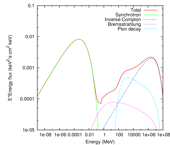
Figure 2.— Emissivities for the four principal processes producing X-ray to gamma-ray emission. Parameters are shown in Table 1.

Table 1Model Parameters: Uniform Medium

Model	$n_{0}$	$s$	$B_{2}$	$\zeta$	$R_{s}$	$t$	$u_{s}$	$E_{me}$	$E_{mi}$
	(cm-3)		($\mu$G)		(cm)	(yr)	(km s-1)	(TeV)	(TeV)
Homogeneous	0.97	2.2	4.5	$10^{-4}$	$2.5\times 10^{19}$	1700	1850	54	137
Sedov analytic (SA)	0.25	2.2	4.5	$10^{-4}$	$2.5\times 10^{19}$	1700	1850	51	429
U1	0.25	2.2	4.5	$10^{-4}$	$2.0\times 10^{19}$	972	2590	76	123
U2	0.25	2.2	4.5	$10^{-4}$	$2.5\times 10^{19}$	1700	1850	54	137
U3	0.25	2.2	4.5	$10^{-4}$	$6.6\times 10^{19}$	21,000	427	43	203

Note. — Models U1, U2, and U3 use the 1-D hydrodynamic simulations.

Table 2Model Parameters: Standard Collision

Model	$n_{0}$	$s$	$B_{2}$	$\zeta$	$R_{s}$	$t$	$u_{s}$	$E_{me}$	$E_{mi}$
	(cm-3)		($\mu$G)		(cm)	(yr)	(km s-1)	(TeV)	(TeV)
Justbefore (JB)	0.25	2.2	4.5	$10^{-4}$	$2.50\times 10^{19}$	1700	1850	54	137
A1	5.0	2.2	20	$10^{-4}$	$2.67\times 10^{19}$	2027	737	22	141
A2	5.0	2.2	20	$10^{-4}$	$2.71\times 10^{19}$	2236	586	14	141
A3	5.0	2.2	20	$10^{-4}$	$2.80\times 10^{19}$	2740	499	12	142
A4	5.0	2.2	20	$10^{-4}$	$2.92\times 10^{19}$	3541	413	9.7	143
A5	5.0	2.2	20	$10^{-4}$	$3.13\times 10^{19}$	5350	318	7.4	143

Note. — In all cavity models, the wall is located at $R_{w}=2.67\times 10^{19}$ cm, with a density jump there of a factor of 20, unless otherwise noted. The collision occurs at a time of about 2000 yr, when the shock velocity is 1690 km s^-1.

4. Results

Images and spectra were calculated for both classes of model: those encountering a uniform medium and those interacting with a cavity wall. In the former case, the remnant dynamics are just those of a Sedov blast wave. Two types of Sedov models are described: one using the analytical Sedov solution and including anisotropies due to magnetic-field variations; and one suitable for the hydrodynamic simulations, in which the magnetic field is assumed isotropized with a strength simply proportional to the square root of density at all times. The former model will be referred to as Sedov, and the latter, models U1, U2, and U3 of Table 1. (Model U2 will be described in particular; it has an age corresponding to a time just before collision with the wall, and is also listed as JB (“just before”) in Table 2.)

For cavity models, we focus on a “standard collision” (SC) scenario, with model parameters given in Table 2. We exhibit results at five times after the collision. More extensive parameter studies can be found in Tang (PhD thesis, in preparation).

4.1. Dynamics

The familiar Sedov dynamical quantities and the radial dependence of magnetic fields are plotted in Figure 3. The field strength governs the electron distribution (through synchrotron losses), and therefore affects the inverse-Compton emissivity as well as the synchrotron emissivity. The total strength assuming flux-freezing (dashed, or blue, or third curve from the top in Fig. 3) is always smaller than that from the simple assumption $B^{2}\propto\rho$, used in the hydrodynamic simulations.

   

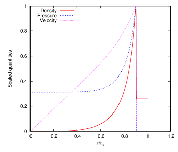
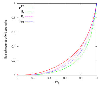
Figure 3.— Left: Scaled profiles of dynamical quantities for Sedov dynamics. Right: Scaled profiles of magnetic-field components for Sedov density profiles. The total magnetic-field strength assuming evolution only due to flux-freezing is the blue (short-dashed) curve, while the approximation of $B\propto\rho^{1/2}$ is shown in red (top, solid curve). Note that the latter is always larger than the former.

4.2. Emission from Sedov-phase remnants

We first compare the analytic Sedov model (SA) with the homogeneous (zero-D) model, then with the numerical model U2.

4.2.1 Spectra

Figure 2 shows spectral fluxes for a homogeneous, spherical remnant with properties shown in Table 2, to be compared with Figure 4. The evolution of magnetic-field strength in the latter model brings about differences of factors of $\sim 3$: while the synchrotron flux at low frequencies is very close to that from a one-zone model, the cutoff frequency (actually a function of position in the SA model) is higher by about a factor of 3. All the gamma-ray fluxes are lower in the SA model by factors of about 3 (a slightly larger factor for inverse-Compton), due to the density dropoff behind the shock and the $n^{2}$ density dependences of those processes. The combination of higher rolloff frequency for the synchrotron component and lower IC normalization makes the ratio of peak synchrotron and IC fluxes differ considerably from that in the one-zone model.

   

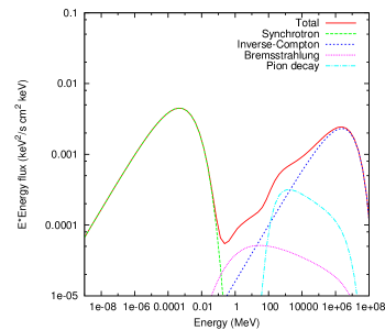
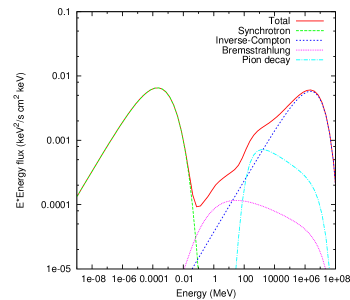
Figure 4.— Left: Fluxes for a model based on Sedov analytic dynamics (parameters shown in Table 1). The magnetic-field spatial variation is the primary reason for differences between this model and the one-zone (zero-D) spectra (Fig. 2). See text for details. Right: Fluxes for the numerical Sedov model with the same input parameters, differing only in the treatment of magnetic field.

The hydrodynamic model before the blast wave encounters the cavity wall (model U2, or JB) is also basically a Sedov model, but differs in the treatment of magnetic field. As Fig. 3 shows, that difference in the remnant interior is substantial. Figure 4 compares the spatially integrated fluxes in the two models. The differences are surprisingly small; the hydrodynamic model does have a higher synchrotron flux, as expected from the somewhat higher magnetic field in the remnant interior. But all flux differences are of order a factor 3 or less.

4.2.2 Images

The anisotropy of the magnetic field in the SA model allows departure from circular symmetry in the images, if not in the dynamics, since the magnetic-field strength affects the maximum energies to which electrons or ions can be accelerated. See Reynolds (2008) for a review. For electrons, if synchrotron losses limit the maximum energy (as is the case for the relatively mature cases considered here), the maximum electron energy $E_{me}$ (actually the $e$-folding energy of a roughly exponential cutoff to the power-law, in simple cases) obeys $E_{me}\propto B^{-1/2}$, so the characteristic synchrotron frequency emitted by such electrons, $\nu_{c}$, obeys $\nu_{c}\propto E_{me}^{2}B$ which is independent of $B$. However, the strength of the synchrotron component does of course depend on the magnetic-field strength. For ions, the most likely mechanism limiting acceleration is the finite size or age of the remnant (roughly equivalent criteria), resulting in $E_{mi}\propto B$ – so higher ion energies can be achieved where the magnetic field is higher. However, higher fields produce lower electron maximum energies since those are loss-limited for the models considered here.

Images for the SA model are shown in Fig. 5. The uniform upstream magnetic field is in the vertical direction in the plane of the figures. The synchrotron emission is brightest near the equators, in a “belt” (as opposed to a “cap”) geometry, simply due to higher synchrotron emissivity where the magnetic field is larger due to compression of the tangential component. The synchrotron emission is confined to a thin region, that becomes thinner for higher photon energies due to downstream energy losses by the electrons (the “thin rims” phenomenon; see R08). The 1 GeV images of IC, electron-ion bremsstrahlung, and $\pi^{0}$ emission are all circularly symmetric. Since the IC emission represents interaction of the electrons with a uniform photon sea (the CMB), there is a slower radial dropoff of emission toward the center than is true for either of the other processes, in which both primary and target populations drop steeply in density toward the remnant center, resulting in a density-squared dependence. (The synchrotron emission varies as the electron density times $B^{1+\alpha}$, and with $\alpha=0.6$ and $B\propto\rho^{1/2}$ in the numerical models, synchrotron emission is also roughly proportional to density squared.)

At 10 TeV, the lower post-shock magnetic field at the poles results in slightly lower maximum ion energies, reducing emission there. Electron maximum energies would be higher (Equation (13)), but the field drops below the value at which the magnetic energy density equals that in CMB photons, so there is a ceiling to electron energies, and the shell emission has a minimum at the poles for very high photon energies. That minimum disappears for larger magnetic-field strengths. Fig. 6 shows radial profiles of those images. The inflection in the IC profile is an artifact, but the general property of much broader profiles in IC than in pion-decay emission is robust and true over a wide range of energies.

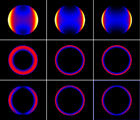
Figure 5.— Images of SA model due to different radiative processes, at different photon energies. Top row: Synchrotron emission at 1 GHz, 1 keV, and 10 keV. Note the thinning of the rim at higher energies. Middle row: IC, bremsstrahlung, and $\pi^{0}$ emission at 1 GeV. The IC shell is broader because the photon target field is uniform, while both bremsstrahlung and $\pi^{0}$ emission targets also scale with density, so the emissivity varies as density squared in the interior. (The apparent smaller size of the IC image is an illusion.) Bottom row: Same processes at 10 TeV. The magnetic field is lowest ($1.4\ \mu$G) at position angles 0 and $180^{\circ}$, so maximum ion energy is lowest there. However, $B$ there is so low that the energy density in CMB photons dominates over magnetic-field energy density, and electron energy losses are dominated by ICCMB interactions. This reduces the maximum electron energy, causing the lower IC emission there.

     

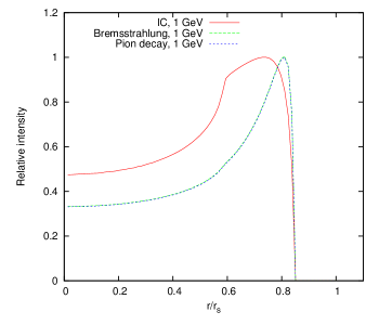
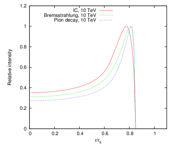
Figure 6.— Left: Radial profiles (along a horizontal or equatorial radius) of the three 1 GeV images in Fig. 5. Right: Same, for 10 TeV images. The bremsstrahlung and $\pi^{0}$ profiles are virtually identical at 1 GeV, but the broader IC profile might make it distinguishable observationally.

4.3. Time evolution

   

   

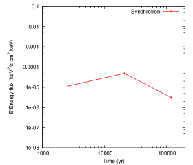
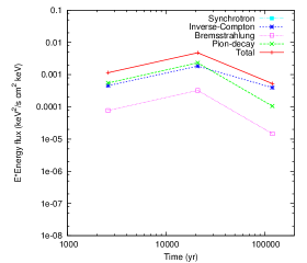
Figure 7.— Fluxes $E^{2}F(E)$ as a function of time, for the uniform-density model. Upper left: 1 GHz. Upper right: 1.33 keV. Lower left: 1 GeV. Lower right: 1 TeV.

Figure 7 shows the time evolution of fluxes (shown as $E^{2}F(E)$ keV² cm^-2 s^-1 keV^-1, where $F(E)$ is the number flux of photons, or $ES(E)$ where $S(E)$ is the energy flux) due to the different radiative processes, for the case of expansion into a uniform medium. While the dynamics are self-similar, the evolution of the electron distribution is not, and there is some structure to the flux evolution, though the variations are not large. At late times, the slowing shock results in both a lower maximum energy for ions, and in fewer relativistic particles. Figure 8 shows SEDs for the three models U1, U2, and U3.

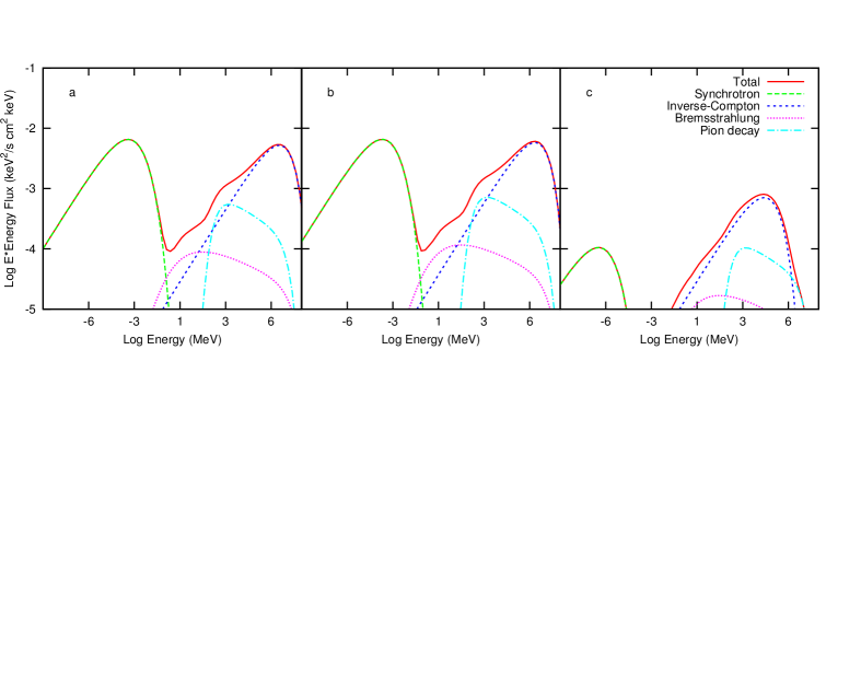
Figure 8.— Spectra of models U1 (a), U2 (b), and U3 (c)). Only at very late times, as exhibited in (c), is there a substantial difference in the spectrum, as the much lower shock velocity greatly reduces the populations of accelerated ions and electrons.

4.4. Collision with cavity wall

For the standard collision model parameters, the collision with the cavity wall occurs at a time of 1990 yr. Figure 9 shows profiles of density, pressure, and velocity just before and just after the collision with the wall. The reflected shock (negative velocities) moves back into the shocked material, while the blast wave moves forward at a much lower velocity, roughly lower as the square root of the higher density.

   

   

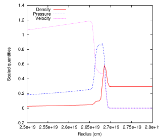
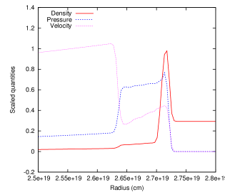
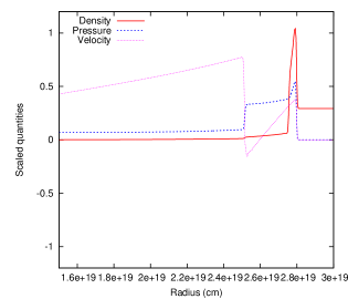
Figure 9.— Four snapshots of the blast wave just after reaching the wall where the density jumps by a factor of 20. The times are 2070, 2210, 2650, and 3530 yr. Densities are in units of $4\times 10^{-23}$ cm^-3, pressures in units of $4\times 10^{-8}$ dyn cm^-2, and velocities in units of $1000$ km s^-1. Note the scale change between the third and fourth panels. The reflected shock accelerates rapidly back toward the remnant center.

4.4.1 Time evolution of spectra

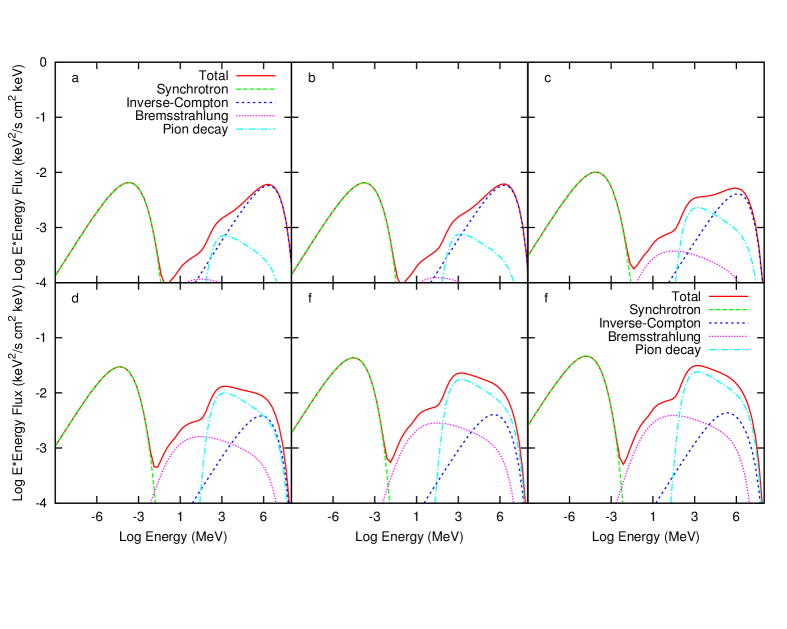
Figure 10.— Spectra as a function of time, for the standard collision model. (a) JB (just before; age 1700 yr); (b) model A1 (2027 yr); (c) model A2 (2236 yr); (d) model A3 (2740 yr); (e) model A4 (3541 yr); (f) model A5 (5350 yr). Note the change in relative strengths of IC and $\pi^{0}$-decay processes with time, causing dramatic changes in the summed spectrum at GeV to TeV energies.

Figure 10 shows the individual spectra at the six times of the standard-collision model listed in Table 2. The synchrotron peak strengthens and moves to lower energies as the shock velocity decreases. However, the major change is in the shape of the GeV-TeV emission, where the increasing relative prominence of $\pi^{0}$ and bremsstrahlung emission relative to inverse-Compton emission causes the shape of the total spectrum to change dramatically with time, from a positive slope (in $E^{2}F(E)$ space) to a steeply negative slope. Since the former two processes basically vary as density squared while the latter only as the first power of density, the much greater density in the wall is responsible for this change.

The SEDs after the collision show significant differences from the JB model shown in Fig. 4, mainly in the gamma-ray regime. The much greater density for targets increases the importance of $\pi^{0}$ emission and bremsstrahlung relative to ICCMB, and the sum actually mimics a power-law with a softer spectrum than that of $\pi^{0}$ emission alone. At a significantly later time, model A5 shows the effects of a slower shock velocity and greater volume of shocked denser material. The slower shock has reduced the maximum electron energy, since it is limited by radiative losses. The maximum ion energy continues to rise, but only slowly, with the increased age almost completely canceled by the slowing shock. The total emission has a significantly steeper slope between 1 GeV and 10 TeV than in model A2, closer to that of $\pi^{0}$-decay alone (but not yet as steep).

4.4.2 Images

Figs. 11 – 15 show model images and profiles. In model A1 (Fig. 11), the emission is dominated by material in the cavity; the shocked wall region is still very thin. The X-ray synchrotron emission is confined to a thinner shell than the radio emission, due to electron energy losses. The IC emission occupies more of the remnant interior because of the dependence on only one power of density. The images at 1 GeV and 1 TeV are very similar and the latter are not shown. The next two sets of images, for models A2 and A3, show the effects of the rapidly increasing emission from shocked wall material. The synchrotron emission is almost totally confined to the region containing shocked wall material, but that emission is much brighter than before; the emission from shocked cavity material is much less prominent by contrast. The $\pi^{0}$ emission (and bremsstrahlung, not shown but indistinguishable from the $\pi^{0}$ morphology) are similarly confined to a thin rim, since their emissivities also depend on the square of density. However, the inverse-Compton emission, which varies only with the first power of density, has a much stronger presence in the remnant interior. In the later models A4 and A5 (Figs. 14 and 15), there are substantial differences in the IC emission between 1 GeV and 1 TeV; at 1 TeV the IC emission actually peaks at the interface between shocked wall material and shocked cavity material, instead of at the outer blast wave, and has a much larger center-to-limb ratio in brightness. The profiles of Figs. 11 – 15 show these effects more clearly.

Model A1 (age 2027 yr)

   

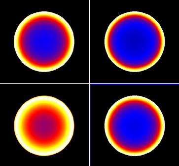
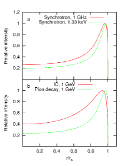
Figure 11.— Images and profiles due to different radiative processes, for model A1. Top row: Synchrotron emission at 1 GHz and 1.33 keV, and profiles (a). Bottom row: IC and $\pi^{0}$ emission at 1 GeV, and profiles (b). The images and profiles for IC and $\pi^{0}$ emission at 1 TeV are indistinguishable from those at 1 GeV, and the bremsstrahlung image is very similar to the $\pi^{0}$-decay image throughout. The color scale is relative to each image maximum.

Model A2 (age 2236 yr)

   

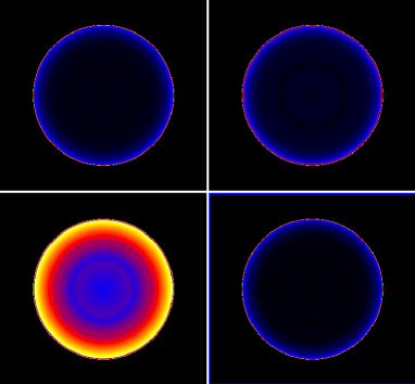
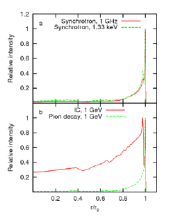
Figure 12.— Images and profiles due to different radiative processes, for model A2. Top row: Synchrotron emission at 1 GHz and 1.33 keV, and profiles (a). Bottom row: IC and $\pi^{0}$ emission at 1 GeV, and profiles (b) (indistinguishable from those at 1 TeV). The small ripples in the IC image are artifacts of the numerical interpolations. Again, the color scale is relative to each image maximum.

Model A3 (age 2740 yr)

   

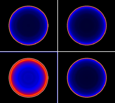
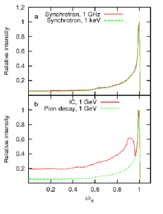
Figure 13.— Images and profiles due to different radiative processes, for model A3. Top row: Synchrotron emission at 1 GHz and 1.33 keV, and profiles (a). Bottom row: IC and $\pi^{0}$ emission at 1 GeV, and profiles (b).

Model A4 (age 3541 yr)

   

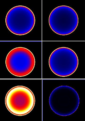
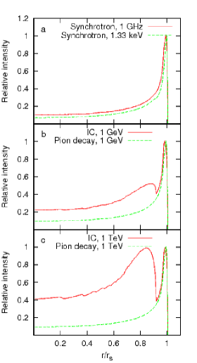
Figure 14.— Images and profiles due to different radiative processes, for model A4. Top row: Synchrotron emission at 1 GHz and 1.33 keV, and profiles (a). Middle row: IC and $\pi^{0}$ emission at 1 GeV, and profiles (b). Bottom row: IC and $\pi^{0}$ emission at 1 TeV, and profiles (c).

Model A5 (age 5350 yr)

   

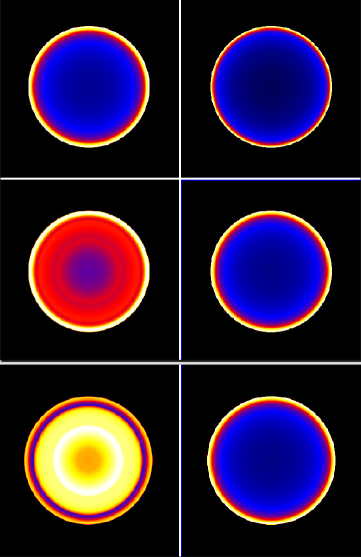
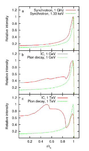
Figure 15.— Images and profiles due to different radiative processes, for model A5. Top row: Synchrotron emission at 1 GHz and 1.33 keV, and profiles (a). Middle row: IC and $\pi^{0}$ emission at 1 GeV, and profiles (b). Bottom row: IC and $\pi^{0}$ emission at 1 TeV, and profiles (c). The bump near $r/r_{s}=0.5$ for IC emission at 1 TeV is an artifact of the numerical interpolations, visible only at the highest energies.

4.5. Time evolution of fluxes

For the standard-collision case, the time variation of fluxes is of course quite different from the uniform-medium case. The fluxes due to the different processes as a function of time are shown in Fig. 16. The time of the collision is 1990 yr, just after the first datapoint. Fluxes rise rapidly thereafter for a few thousand years, eventually resuming the decline due to expansion and slowing shock velocity. At the latest times, the IC process has the slowest decline rate and comes to dominate the integrated spectrum, as also shown in the spectra (Fig. 10). At those times, the synchrotron peak has moved to low enough energies that there is negligible X-ray synchrotron emission, though the gamma-ray emission is still quite significant.

   

   

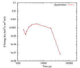
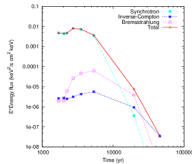
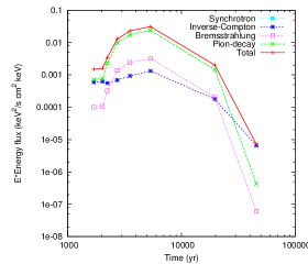
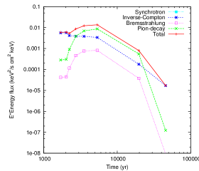
Figure 16.— Fluxes as a function of time, for the standard collision model. Upper left: 1 GHz. Upper right: 1.33 keV. Lower left: 1 GeV. Lower right: 1 TeV.

5. Discussion

The comparison of one-zone to 1-D models shows significant differences, and not just in the obvious shell morphology of the latter. Even in the uniform-medium case, variations in integrated fluxes of factors of several occur, as described above. However, with the interaction with the cavity wall, much greater differences appear. In morphology, the four processes fall into three classes: (1) synchrotron, (2) bremsstrahlung and $\pi^{0}$-decay, and (3) IC. Differences betweeen the first two are slight, since the emissivity of synchrotron emission varies approximately as density squared, as do those of bremsstrahlung and $\pi^{0}$-decay. IC from CMB photons, however, depends on only one power of density. Thus, as the remnant encounters the cavity wall, emission from the cavity material becomes essentially negligible for all but IC, but the latter shows enough central emission that a double-shell structure can even emerge (Figs. 14 and 15). Note that unless the self-generated radiation field of the remnant is extremely intense, this would still be true even in the presence of IC from optical-IR seed photon fields in addition to the CMB, as those radiation energy densities are not expected to vary much over the remnant volume.

This strong morphological difference has spectral consequences as well. Figure 17 compares the emission after the collision with the wall (model A3, age 2740 yr) with that from a homogeneous (one-zone) model with the parameters of the current blast wave. The cavity in the past of model A3 substantially reduces the emission at all wavelengths, but also changes the relative weights of the different processes. The higher relative weight of IC emission in model A3 causes the slope of the GeV-TeV part of the spectrum to be substantially flatter than for the one-zone model. Clearly, attempting to describe a radially varying source with the properties of the current blast wave would result in incorrect inferences of several parameters.

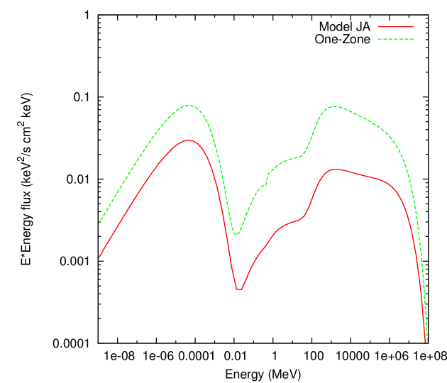
Figure 17.— Comparison of the integrated spectrum of model A3 with that from a homogeneous (one-zone) model using the parameters of the forward blast wave (in the dense medium).

Figure 10 shows that the total gamma-ray emission from model A2 is dominated by $\pi^{0}$-decay at GeV energies and by IC at TeV energies. This implies also a strong morphological variation of the source with energy. Fig. 18 shows the total emission at 1 GeV and at 1 TeV, along with radial profiles of each. While the thin shell of shocked wall material is distinguishable in these high-resolution calculations, such angular resolution will not be available in this spectral regime for the foreseeable future. However, even very coarse angular resolution can distinguish the much greater central emission from the 1 TeV image, and such morphological differences between GeV and TeV-range images are powerful clues to the importance of hadronic vs. leptonic processes in cavity SNRs.

   

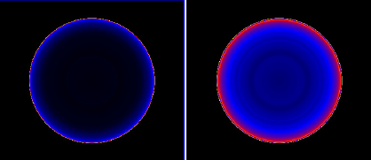
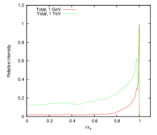
Figure 18.— Images of the total emission from model A2 (age 2236 yr) at 1 GeV (left) and 1 TeV (center), and profiles of each (right). Images have $768\times 768$ resolution.

6. Summary and conclusions

As angular resolutions and sensitivities of gamma-ray observations of supernova remnants continue to improve, models will need to increase in sophistication to allow appropriate interpretation of such new observations. We have systematically investigated the differences between homogeneous (one-zone) models and those with radial variations (spherical symmetry), for the remnant phases starting with times when ejecta emission becomes unimportant, through the onset of radiative cooling (Sedov blast waves, for power-law external media). For the case of a uniform external medium, analytic dynamics were used and compared with results from hydrodynamic simulations. For an explosion in a constant-density cavity bounded by a wall of constant density 20 times larger, hydrodynamic simulations in spherical symmetry were performed using the VH-1 code. In both cases, the blast wave was assumed to accelerate $10^{-4}$ of the ions with momenta greater than ten times thermal (i.e., $10m_{p}v_{\rm shock}$) to a power-law energy distribution with power-law index 2.2; electrons were assumed to have the same energy distribution with a normalization of 0.02 times that of ions. Both distributions were cut off exponentially at a maximum energy limited by the remnant age, or for electrons, at a maximum energy limited by radiative losses if lower. Emission from these distributions was calculated due to synchrotron radiation, electron-ion and electron-electron bremsstrahlung, and inverse-Compton upscattering of cosmic microwave background photons (ICCMB). More extensive sets of models, also showing the effects of variations of parameters, are included in Tang (2016; PhD thesis, in preparation).

We find that for a uniform external medium, aside from obvious morphological differences, one-zone models differ from 1-D spherical models in integrated fluxes by factors of several. Ratios of emission due to different processes could differ by a somewhat larger factor.

We followed the time evolution of spectra, total fluxes, and remnant morphology as the blast wave interacted with the cavity wall. Here, use of the current shock wave properties (shock speed and immediate postshock density) in a one-zone model would produce substantially different predictions compared to those of the cavity model. Furthermore, the time evolution of the spectrum at GeV – TeV energies is such that apparent power-laws of different slope (and even different sign, in $E^{2}F(E)$ space) appear at different times, even though the basic input spectrum does not change. Interpretation of slopes of power-law fits at gamma-ray energies should be undertaken with great care; such slopes may not reflect the energy distribution of a single underlying particle population.

Cavity-wall interactions produced striking morphological effects, from significant variations of morphology with energy, to double-shell structures which could potentially be resolvable. Even with shock velocities as low as a few hundred km s^-1, significant gamma-ray emission, diagnostic of interactions with material with radially varying density, can occur in older SNRs. Such objects should be targets of future observations with both current observatories such as Fermi and H.E.S.S., and future ones such as CTA.

We would like to thank NASA for support of this project through Fermi Guest Investigator Program award 61101. We gratefully acknowledge assistance from John Blondin on VH-1 issues.

References

- Abdo et al. (2009) Abdo, A. A., Ackermann, M., Ajello, M., et al. 2009, ApJ, 706, L1
- Abdo et al. (2010) —. 2010, ApJ, 718, 348
- Abdo et al. (2011) —. 2011, ApJ, 734, 28
- Acciari et al. (2010) Acciari, V. A., Aliu, E., Arlen, T., et al. 2010, ApJ, 714, 163
- Ackermann et al. (2013) Ackermann, M., Ajello, M., Allafort, A., et al. 2013, Science, 339, 807
- Araya & Cui (2010) Araya, M., & Cui, W. 2010, ApJ, 720, 20
- Atoyan & Dermer (2012) Atoyan, A., & Dermer, C. D. 2012, ApJ, 749, L26
- Baring et al. (1999) Baring, M. G., Ellison, D. C., Reynolds, S. P., Grenier, I. A., & Goret, P. 1999, ApJ, 513, 311
- Berezhko & Völk (2008) Berezhko, E. G., & Völk, H. J. 2008, A&A, 492, 695
- Blondin et al. (1998) Blondin, J. M., Wright, E. B., Borkowski, K. J., & Reynolds, S. P. 1998, ApJ, 500, 342
- Colella & Woodward (1984) Colella, P., & Woodward, P. R. 1984, J.Comp.Phys., 54, 174
- Duin & Strom (1975) Duin, R. M., & Strom, R. G. 1975, A&A, 39, 33
- Dwarkadas (2005) Dwarkadas, V. V. 2005, ApJ, 630, 892
- Ellison et al. (2012) Ellison, D. C., Slane, P., Patnaude, D. J., & Bykov, A. M. 2012, ApJ, 744, 39
- Giordano et al. (2012) Giordano, F., Naumann-Godo, M., Ballet, J., et al. 2012, ApJL, 744, L2
- Haug (1975) Haug, E. 1975, Z.Naturforsch.A, 30, 1099
- Hewitt et al. (2012) Hewitt, J. W., Grondin, M.-H., Lemoine-Goumard, M., et al. 2012, ApJ, 759, 89
- Houck & Allen (2006) Houck, J. C., & Allen, G. E. 2006, ApJS, 167, 26
- Jokipii (1987) Jokipii, J. R. 1987, ApJ, 313, 842
- Katagiri et al. (2011) Katagiri, H., Tibaldo, L., Ballet, J., et al. 2011, ApJ, 741, 44
- Koyama et al. (1995) Koyama, K., Petre, R., Gotthelf, E. V., et al. 1995, Nature, 378, 255
- Lee et al. (2013) Lee, S.-H., Slane, P. O., Ellison, D. C., Nagataki, S., & Patnaude, D. J. 2013, ApJ, 767, 20
- Morlino & Caprioli (2012) Morlino, G., & Caprioli, D. 2012, A&A, 538, A81
- Pacholczyk (1970) Pacholczyk, A. G. 1970, Radio astrophysics. Nonthermal processes in galactic and extragalactic sources (San Franciso: Freeman)
- Reynolds (1998) Reynolds, S. P. 1998, ApJ, 493, 375
- Reynolds (2008) —. 2008, ARA&A, 46, 89
- Reynolds & Chevalier (1981) Reynolds, S. P., & Chevalier, R. A. 1981, ApJ, 245, 912
- Rieger et al. (2013) Rieger, F. M., de Oña-Wilhelmi, E., & Aharonian, F. A. 2013, Frontiers of Physics, 8, 714
- Shklovsky (1953) Shklovsky, I. S. 1953, Doklady Akad.Nauk.SSR, 91, 475
- Tenorio-Tagle et al. (1990) Tenorio-Tagle, G., Bodenheimer, P., Franco, J., & Rozyczka, M. 1990, MNRAS, 244, 563
- Tenorio-Tagle et al. (1991) Tenorio-Tagle, G., Rozyczka, M., Franco, J., & Bodenheimer, P. 1991, MNRAS, 251, 318
- Uchiyama et al. (2010) Uchiyama, Y., Blandford, R. D., Funk, S., Tajima, H., & Tanaka, T. 2010, ApJ, 723, L122
- van Marle & Keppens (2012) van Marle, A. J., & Keppens, R. 2012, A&A, 547, A3
- van Marle et al. (2015) van Marle, A. J., Meliani, Z., & Marcowith, A. 2015, A&A, 584, A49