Orthogonal Tree Decompositions of Graphs

Vida Dujmović   Gwenaël Joret   Pat Morin   Sergey Norin   David R. Wood 

Abstract. This paper studies graphs that have two tree decompositions with the property that every bag from the first decomposition has a bounded-size intersection with every bag from the second decomposition. We show that every graph in each of the following classes has a tree decomposition and a linear-sized path decomposition with bounded intersections: (1) every proper minor-closed class, (2) string graphs with a linear number of crossings in a fixed surface, (3) graphs with linear crossing number in a fixed surface. Here ‘linear size’ means that the total size of the bags in the path decomposition is $O(n)$ for $n$-vertex graphs. We then show that every $n$-vertex graph that has a tree decomposition and a linear-sized path decomposition with bounded intersections has $O(\sqrt{n})$ treewidth. As a corollary, we conclude a new lower bound on the crossing number of a graph in terms of its treewidth. Finally, we consider graph classes that have two path decompositions with bounded intersections. Trees and outerplanar graphs have this property. But for the next most simple class, series parallel graphs, we show that no such result holds.

1 Introduction

A tree decomposition represents the vertices of a graph as subtrees of a tree, so that the subtrees corresponding to adjacent vertices intersect. The treewidth of a graph $G$ is the minimum taken over all tree decompositions of $G$, of the maximum number of pairwise intersecting subtrees minus 1. Treewidth measures how similar a given graph is to a tree. It is a key measure of the complexity of a graph and is of fundamental importance in algorithmic graph theory and structural graph theory. For example, treewidth is a key parameter in Robertson–Seymour graph minor theory [48], and many NP-complete problems are solvable in polynomial time on graphs of bounded treewidth [14].

The main idea in this paper is to consider two tree decompositions of a graph, and then measure the sizes of the intersection of bags from the first decomposition with bags from the second decomposition. Intuitively, one can think of the bags from the first decomposition as being horizontal, and the bags from the second decomposition as being vertical, so that the two tree decompositions are ‘orthogonal’ to each other. We are interested in which graphs have two tree decompositions such that every bag from the first decomposition has a bounded-size intersection with every bag from the second decomposition. This idea is implicit in recent work on layered tree decompositions (see Section 2), and was made explicit in the recent survey by Norin [44].

Grid graphs illustrate this idea well; see Figure 1. Say $G$ is the $n\times n$ planar grid graph. The sequence of consecutive pairs of columns determines a tree decomposition, in fact, a path decomposition with bags of size $2n$. Similarly, the sequence of consecutive pairs of rows determines a path decomposition with bags of size $2n$. Observe that the intersection of a bag from the first decomposition with a bag from the second decomposition has size 4. It is well known [34] that $G$ has treewidth $n$, which is unbounded. But as we have shown, $G$ has two tree decompositions with bounded intersections. This paper shows that many interesting graph classes with unbounded treewidth have two tree decompositions with bounded intersections (and with other useful properties too).

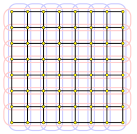
Figure 1: Two 4-orthogonal path decompositions of the grid graph.

Before continuing, we formalise these ideas. A tree decomposition of a graph $G$ is given by a tree $T$ whose nodes index a collection $(T_{x}\subseteq V(G):x\in V(T))$ of sets of vertices in $G$ called bags, such that (1) for every edge $vw$ of $G$, some bag $T_{x}$ contains both $v$ and $w$, and (2) for every vertex $v$ of $G$, the set $\{x\in V(T):v\in T_{x}\}$ induces a non-empty (connected) subtree of $T$. For brevity, we say that $T$ is a tree decomposition (with the bags $T_{x}$ implicit). The width of a tree decomposition $T$ is $\max\{|T_{x}|-1:x\in V(T)\}$, and the treewidth $\operatorname{tw}(G)$ of a graph $G$ is the minimum width of the tree decompositions of $G$. A path decomposition is a tree decomposition in which the underlying tree is a path. We describe a path decomposition simply by the corresponding sequence of bags. The pathwidth $\operatorname{pw}(G)$ of a graph $G$ is the minimum width of the path decompositions of $G$. Two tree decompositions $A$ and $B$ of a graph $G$ are $c$-orthogonal if $|A_{x}\cap B_{y}|\leqslant c$ for all $x\in V(A)$ and $y\in V(B)$.

It turns out that not only the size of bag intersections is important when considering orthogonal tree decompositions. A key parameter is the total size of the bags in a tree decomposition $T$, which we call the magnitude, formally defined to be $\sum_{x\in V(T)}|T_{x}|$. For example, consider the complete bipartite graph $K_{n,n}$. Say $V=\{v_{1},\dots,v_{n}\}$ and $W=\{w_{1},\dots,w_{n}\}$ are the two colour classes. Then

$$P =(V\cup\{w_{1}\},V\cup\{w_{2}\},\dots,V\cup\{w_{n}\})\text{ and }$$

$$Q =(W\cup\{v_{1}\},W\cup\{v_{2}\},\dots,W\cup\{v_{n}\})$$

are path decompositions of $K_{n,n}$, such that the intersection of each bag of $P$ with each bag of $Q$ has exactly two vertices. However, both $P$ and $Q$ have magnitude $n(n+1)$. On the other hand, we prove in Section 3 that if two tree decompositions of a graph $G$ have bounded intersections and one has linear magnitude, then $G$ has a linear number of edges. Here ‘linear’ means $O(n)$ for $n$-vertex graphs.

Our main results show that every graph in each of the following classes has a tree decomposition and a linear-magnitude path decomposition with bounded intersections:

• every proper minor-closed class (Section 4),

• string graphs with a linear number of crossings in a fixed surface (Section 5),

• graphs with linear crossing number in a fixed surface (Section 6),

The latter two examples highlight that orthogonal decompositions are of interest well beyond the world of minor-closed classes. We also show that every graph that has a tree decomposition and a linear-magnitude path decomposition with bounded intersections has $O(\sqrt{n})$ treewidth. This result is immediately applicable to each of the above three classes. As a corollary, we conclude a new lower bound on the crossing number of a graph in terms of its treewidth (Section 6).

Treewidth is intrinsically related to graph separators. A set $S$ of vertices in a graph $G$ is a separator of $G$ if each component of $G-S$ has at most $\tfrac{1}{2}|V(G)|$ vertices. Graphs with small treewidth have small separators, as shown by the following result of Robertson and Seymour [49]:

Lemma 1 ([49]).

Every graph $G$ has a separator of size at most $\operatorname{tw}(G)+1$.

Our treewidth bounds and Lemma 1 give $O(\sqrt{n})$ separator results for each of the above three classes. Also note that a converse to Lemma 1 holds: graphs in which every subgraph has a small separator have small treewidth [23, 47].

The paper then considers graph classes that have two path decompositions with bounded intersections. Trees and outerplanar graphs have this property. But for the next most simple class, series parallel graphs, we show that no such result holds (Section 7). The paper concludes by discussing connections between orthogonal tree decompositions and boxicity (Section 8) and graph colouring (Section 9).

2 Layered Treewidth

The starting point for the study of orthogonal tree decompositions is the notion of a layered tree decomposition, introduced independently by Dujmović et al. [22] and Shahrokhi [55]. Applications of layered treewidth include nonrepetitive graph colouring [22], queue layouts, track layouts and 3-dimensional graph drawings [22], book embeddings [21], and intersection graph theory [55].

A layering of a graph $G$ is a partition $(V_{0},V_{1},\dots,V_{t})$ of $V(G)$ such that for every edge $vw\in E(G)$, if $v\in V_{i}$ and $w\in V_{j}$, then $|i-j|\leqslant 1$. Each set $V_{i}$ is called a layer. For example, for a vertex $r$ of a connected graph $G$, if $V_{i}$ is the set of vertices at distance $i$ from $r$, then $(V_{0},V_{1},\dots)$ is a layering of $G$.

The layered width of a tree decomposition $(T_{x}:x\in V(T))$ of a graph $G$ is the minimum integer $\ell$ such that, for some layering $(V_{0},V_{1},\dots,V_{t})$ of $G$, each bag $T_{x}$ contains at most $\ell$ vertices in each layer $V_{i}$. The layered treewidth of a graph $G$ is the minimum layered width of a tree decomposition of $G$. Note that the trivial layering with all vertices in one layer shows that layered treewidth is at most treewidth plus 1. The layered pathwidth of a graph $G$ is the minimum layered width of a path decomposition of $G$; see [3].

While $n$-vertex planar graphs may have treewidth as large as $\sqrt{n}$, Dujmović et al. [22] proved the following:

Theorem 2 ([22]).

Every planar graph has layered treewidth at most $3$. More generally, every graph with Euler genus $g$ has layered treewidth at most $2g+3$.

Layered treewidth is related to local treewidth, which was first introduced by Eppstein [25] under the guise of the ‘treewidth-diameter’ property. A graph class $\mathcal{G}$ has bounded local treewidth if there is a function $f$ such that for every graph $G$ in $\mathcal{G}$, for every vertex $v$ of $G$ and for every integer $r\geqslant 0$, the subgraph of $G$ induced by the vertices at distance at most $r$ from $v$ has treewidth at most $f(r)$; see [32, 15, 17, 25]. If $f(r)$ is a linear function, then $\mathcal{G}$ has linear local treewidth. Dujmović et al. [22] observed that if every graph in some class $\mathcal{G}$ has layered treewidth at most $k$, then $\mathcal{G}$ has linear local treewidth with $f(r)\leqslant k(2r+1)-1$. Dujmović et al. [22] also proved the following converse result for minor-closed classes, where a graph $G$ is apex if $G-v$ is planar for some vertex $v$. (Earlier, Eppstein [25] proved that (b) and (d) are equivalent, and Demaine and Hajiaghayi [17] proved that (b) and (c) are equivalent.)

Theorem 3 ([22, 17, 25]).

The following are equivalent for a minor-closed class $\mathcal{G}$ of graphs:

1. $\mathcal{G}$ has bounded layered treewidth.

2. $\mathcal{G}$ has bounded local treewidth.

3. $\mathcal{G}$ has linear local treewidth.

4. $\mathcal{G}$ excludes some apex graph as a minor.

Dujmović et al. [20] observed that such a converse result does not hold for non-minor-closed classes. In particular, 3-dimensional grid graphs have quadratic local treewidth and unbounded layered treewidth.

A number of non-minor-closed classes also have bounded layered treewidth. Dujmović et al. [20] gave the following two examples. A graph is $(g,k)$-planar if it can be drawn in a surface of Euler genus at most $g$ with at most $k$ crossings on each edge. Dujmović et al. [20] determined an optimal bound on the layered treewidth and treewidth of such graphs.

Theorem 4 ([20]).

Every $(g,k)$-planar graph $G$ has layered treewidth at most $(4g+6)(k+1)$ and treewidth at most $2\sqrt{(4g+6)(k+1)n}$. Conversely, for all $g,k\geqslant 0$ and infinitely many $n$ there is an $n$-vertex $(g,k)$-planar graph with treewidth $\Omega(\sqrt{(g+1)(k+1)n})$ and layered treewidth $\Omega((g+1)(k+1))$.

Map graphs are defined as follows. Start with a graph $G_{0}$ embedded in a surface of Euler genus $g$, with each face labelled a ‘nation’ or a ‘lake’, where each vertex of $G_{0}$ is incident with at most $d$ nations. Define a graph $G$ whose vertices are the nations of $G_{0}$, where two vertices are adjacent in $G$ if the corresponding faces in $G_{0}$ share a vertex. Then $G$ is called a $(g,d)$-map graph. A $(0,d)$-map graph is called a (plane) $d$-map graph; such graphs have been extensively studied [28, 12, 16, 13, 11]. It is easily seen that $(g,3)$-map graphs are precisely the graphs of Euler genus at most $g$ [13, 20]. So $(g,d)$-map graphs provide a natural generalisation of graphs embedded in a surface. Note that if a vertex of $G_{0}$ is incident with $d$ nations, then $G$ contains $K_{d}$, which need not be bounded by a function of $g$. Dujmović et al. [20] determined an optimal bound on the layered treewidth and treewidth of such graphs.

Theorem 5 ([20]).

Every $(g,d)$-map graph on $n$ vertices has layered treewidth at most $(2g+3)(2d+1)$ and treewidth at most $2\sqrt{(2g+3)(2d+1)n}$. Moreover, for all $g\geqslant 0$ and $d\geqslant 8$, for infinitely many integers $n$, there is an $n$-vertex $(g,d)$-map graph with treewidth at least $\Omega(\sqrt{(g+1)dn})$ and layered treewidth at least $\Omega((g+1)d)$.

Theorem 3 leads to further results. A tree decomposition is domino if every vertex is in at most two bags [7, 6, 60].

Lemma 6.

Every graph $G$ with layered treewidth $k$ has a domino path decomposition $P$ and a tree decomposition $T$ such that for every vertex $v$ of $G$, if $G_{v}$ is the subgraph of $G$ induced by the union of the bags of $P$ that contain $v$, then $T$ restricted to $G_{v}$ has width at most $3k-1$.

Proof.

Let $T$ be a tree decomposition of $G$ with layered width $k$ with respect to some layering $V_{1},\dots,V_{t}$ of $G$, where $V_{t}=\emptyset$. Then $P:=(V_{1}\cup V_{2},V_{2}\cup V_{3},\dots,V_{t-1}\cup V_{t})$ is a path decomposition of $G$. Consider a vertex $v\in V_{i}$ for some $i\in[t-1]$. Then $v$ is in exactly two bags, $V_{i-1}\cup V_{i}$ and $V_{i}\cup V_{i+1}$. Thus $P$ is domino. The union of the bags that contain $v$ is $V_{i-1}\cup V_{i}\cup V_{i+1}$, which contains at most $3k$ vertices in each bag of $T$. ∎

Theorems 3 and 6 imply:

Theorem 7.

For every fixed apex graph $H$, there is a constant $k$, such that every $H$-minor-free graph $G$ has a domino path decomposition $P$ and a tree decomposition $T$ such that for every vertex $v$ of $G$, if $G_{v}$ is the subgraph of $G$ induced by the union of the bags of $P$ that contain $v$, then $T$ restricted to $G_{v}$ has width at most $3k-1$.

This result is best possible in the following sense. Let $G$ be obtained from the $n\times n$ grid graph by adding one dominant vertex $v$. Say $T_{1}$ and $T_{2}$ are tree decompositions of $G$. The bags of $T_{1}$ that contain $v$ induce a subgraph that contains the $n\times n$ grid, and therefore has treewidth at least $n$, which is unbounded.

3 Extremal Questions and Treewidth Bounds

We start this section by considering the natural extremal question: what is the maximum number of edges in an $n$-vertex graph that has two orthogonal tree decompositions of a particular type? Dujmović et al. [22] proved that every $n$-vertex graph with layered treewidth $k$ has minimum degree at most $3k-1$ and thus has at most $(3k-1)n$ edges, which is tight up to a lower order term. More general structures allow for quadratically many edges. For example, $K_{n,n}$ has two 2-orthogonal path decompositions, as shown in Section 1. Note that each of these decompositions has quadratic magnitude. We now show that a limit on the magnitude of one decomposition leads to a linear bound on the number of edges, even for tree decompositions.

Lemma 8.

Let $S$ and $T$ be $k$-orthogonal tree decompositions of a graph $G$, where $S$ has magnitude $s$. Then $|E(G)|\leqslant(k-1)s$. In particular, if $s\leqslant c|V(G)|$ then $|E(G)|\leqslant c(k-1)|V(G)|$.

Proof.

Each edge of $G$ is in $G[S_{x}]$ for some $x\in V(S)$. Since $T$ restricted to $G[S_{x}]$ has treewidth at most $k-1$, it follows that $G[S_{x}]$ has less than $(k-1)|S_{x}|$ edges. Thus

$$|E(G)|\leqslant\sum_{x}|E(G[S_{x}])|\leqslant\sum_{x}(k-1)|S_{x}|=(k-1)s.\qed$$

One application of layered treewidth is that it leads to $O(\sqrt{n})$ treewidth bounds.

Theorem 9 (Norine; see [22]).

For every $n$-vertex graph $G$ with layered treewidth $k$,

$$\operatorname{tw}(G)\leqslant 2\sqrt{kn}-1.$$

As an example, Theorems 2 and 9 imply that graphs with bounded Euler genus have treewidth $O(\sqrt{n})$. Dujmović et al. [20] observed that a standard trick applied with Theorem 9 implies:

Theorem 10 ([20]).

For every $n$-vertex graph $G$ with layered treewidth $k$,

$$\operatorname{pw}(G)\leqslant 11\sqrt{kn}-1.$$

We now generalise these results to the setting of orthogonal decompositions. A weak path decomposition of a graph $G$ is a sequence $P_{1},\dots,P_{t}$ of sets of vertices of $G$ called bags, such that $P_{1}\cup\dots\cup P_{t}=V(G)$, for every vertex $v$ of $G$ the set of bags that contain $v$ forms a subsequence, and for every edge $vw$ of $G$, both $v$ and $w$ are in $P_{i}\cup P_{i+1}$ for some $i\in\{1,\dots,t\}$ (where $P_{t+1}$ means $\emptyset$). Note that a path decomposition is a weak path decomposition in which the final condition is strengthened to say that both $v$ and $w$ are in $P_{i}$ for some $i\in\{1,\dots,t\}$. If $P_{1},\dots,P_{t}$ is a weak path decomposition, then $P_{1}\cup P_{2},P_{2}\cup P_{3},\dots,P_{t-1}\cup P_{t}$ is a path decomposition with at most twice the width of $P_{1},\dots,P_{t}$. In this sense, there is little difference between weak path decompositions and path decompositions. The magnitude of a weak path decomposition $P_{1},\dots,P_{t}$ is $\sum_{i\in[n]}|P_{i}|$.

Observe that a layering is a weak path decomposition in which each vertex is in exactly one bag. Thus weak path decompositions with linear magnitude generalise the notion of a layering. In a weak path decomposition, each bag $P_{i}$ separates $P_{1}\cup\dots\cup P_{i-1}$ and $P_{i+1}\cup\dots\cup P_{t}$; that is, there is no edge between $P_{1}\cup\dots\cup P_{i-1}$ and $P_{i+1}\cup\dots\cup P_{t}$. This property is the key to the next lemma, which generalises Theorem 9 to the setting of weak path decompositions. A tree decomposition $T$ and weak path decomposition $P_{1},\dots,P_{t}$ of a graph $G$ are $c$-orthogonal if $|T_{x}\cap P_{i}|\leqslant c$ for all $x\in V(T)$ and $i\in[t]$.

Lemma 11.

Suppose that $T$ is a tree decomposition and $P$ is a weak path decomposition of a graph $G$, where $T$ and $P$ are $k$-orthogonal and $P$ has magnitude $s$. Then

$$\operatorname{tw}(G)\leqslant 2\sqrt{ks}-1.$$

Proof.

Let $t:=\lceil{\sqrt{s/k}}\rceil$. Label the bags of $P$ in order by $1,\dots,t,1,\dots,t,\dots$. Since the magnitude of $P$ is $s$, for some $i\in\{1,\dots,t\}$ the bags labelled $i$ have total size at most $s/t$. Let $G^{\prime}$ be the subgraph of $G$ obtained by deleting the bags labelled $i$. Since each bag of $P$ separates the bags of $P$ before and after it, each connected component of $G^{\prime}$ is contained within $t-1$ consecutive bags of $P$. Thus $G^{\prime}$ has a tree decomposition with bags of size at most $(t-1)k$. Add all the vertices in bags of $P$ labelled $i$ to every bag of this tree decomposition of $G^{\prime}$. We obtain a tree decomposition of $G$ with bag size at most $(t-1)k+s/t\leqslant 2\sqrt{ks}$. Thus $\operatorname{tw}(G)\leqslant 2\sqrt{ks}-1$. ∎

Several comments on Lemma 11 are in order.

First we show that Lemma 11 cannot be strengthened for two tree decompositions with bounded intersections. Let $G$ be a bipartite graph with bipartition $(A,B)$ and maximum degree $\Delta$. Let $S$ be the star decomposition of $G$ with root bag $A$ and a leaf bag $N[w]$ for each vertex $w\in B$. Symmetrically, let $T$ be the star decomposition of $G$ with root bag $B$ and a leaf bag $N[v]$ for each vertex $v\in A$. Observe that $S$ and $T$ are $\Delta$-orthogonal and both have magnitude $|V(G)|+|E(G)|$. Now, apply this construction with $G$ a random cubic bipartite graph on $n$ vertices. We obtain two $3$-orthogonal tree decompositions of $G$ both with magnitude $\frac{5}{2}n$. But it is well known that $G$ has treewidth $\Omega(n)$; see [33] for example. Thus Lemma 11 does not hold for two tree decompositions with bounded intersections.

We now show that Lemma 11 proves that certain graph classes have bounded expansion. A graph class $\mathcal{C}$ has bounded expansion if there exists a function $f$ such that for every graph $G\in\mathcal{C}$, for every subgraph $G^{\prime}$ of $G$, and for all pairwise disjoint balls $B_{1},\dots,B_{s}$ of radius at most $r$ in $G^{\prime}$, the graph obtained from $G^{\prime}$ by contracting each $B_{i}$ into a vertex has average degree at most $f(r)$. If $f(r)$ is a linear or polynomial function, then $\mathcal{C}$ has linear or polynomial expansion, respectively. See [43] for background on graph classes with bounded expansion. Dujmović et al. [22] proved that graphs with bounded layered treewidth have linear expansion. In particular, in a graph of layered treewidth $k$ contracting disjoint balls of radius $r$ gives a graph of layered treewidth at most $(4r+1)k$, and thus with average degree $O(rk)$. This result can be extended as follows. A class $\mathcal{G}$ of graphs is hereditary if for every graph $G\in\mathcal{G}$ every induced subgraph of $G$ is in $\mathcal{G}$. Dvořák and Norin [24] proved that for a hereditary graph class $\mathcal{G}$, if every graph $G\in\mathcal{G}$ has a separator of order $O(|V(G)|^{1-\epsilon})$ for some fixed $\epsilon>0$, then $\mathcal{G}$ has polynomial expansion. Lemmas 11 and 1 then imply the following.

Proposition 12.

Let $\mathcal{G}_{k}$ be the class of graphs $G$ such that every subgraph $G^{\prime}$ of $G$ has a path decomposition with magnitude at most $k|V(G^{\prime})|$ and a tree decomposition that are $k$-orthogonal. Then $\mathcal{G}_{k}$ has polynomial expansion.

We now show that Proposition 12 cannot be extended to the setting of two tree decompositions with bounded intersections. Let $G$ be the 1-subdivision of $K_{n,n}$, which has $N=n^{2}+2n$ vertices. Say the bipartition classes of $K_{n,n}$ are $V:=\{v_{1},\dots,v_{n}\}$ and $W:=\{w_{1},\dots,w_{n}\}$. Let $x_{i,j}$ be the division vertex for edge $v_{i}w_{j}$. Let $S$ be the star decomposition of $G$ with root bag $\{v_{1},\dots,v_{n}\}$, and for each $j\in[n]$ have a leaf bag $V\cup\{w_{j},x_{1,j},\dots,x_{n,j}\}$. Similarly, let $T$ be the star decomposition of $G$ with root bag $W$, and for each $i\in[n]$ have a leaf bag $W\cup\{v_{i},x_{i,1},\dots,x_{i,n}\}$. Then the intersection of a bag from $S$ and a bag from $T$ has size at most $3$. Each of $S$ and $T$ have magnitude $O(N)$. On the other hand, contracting the edges incident to each vertex $v_{i}$ gives $K_{n,n}$ which has unbounded average degree. Thus the class of 1-subdivisions of balanced complete bipartite graphs does not have bounded expansion, but every graph in the class has two tree decompositions with bounded intersections and linear magnitude.

Finally, we consider bounds on pathwidth. It is well known that hereditary graph classes with treewidth $O(n^{\epsilon})$, for some fixed $\epsilon\in(0,1)$, have pathwidth $O(n^{\epsilon})$; see [5, 20] for example. In particular, Lemma 11 and Lemma 6.1 of Dujmović et al. [20] imply the following.

Lemma 13.

Let $\mathcal{G}$ be a hereditary class of graphs, such that every $n$-vertex graph $G$ in $\mathcal{G}$ has a tree decomposition $T$ and a weak path decomposition $P$, such that $T$ and $P$ are $k$-orthogonal and $P$ has magnitude at most $cn$. Then for every $n$-vertex graph $G$ in $\mathcal{G}$,

$$\operatorname{pw}(G)\leqslant 11\sqrt{ckn}-1.$$

4 Minor-Closed Classes

This section shows that graphs in a fixed minor-closed class have a tree decomposition and a linear-magnitude path decomposition with bounded intersections. The following graph minor structure theorem by Robertson and Seymour is at the heart of graph minor theory. In a tree decomposition $T$ of a graph $G$, the torso of a bag $T_{x}$ is the subgraph obtained from $G[T_{x}]$ by adding, for each edge $xy\in E(T)$, all edges $vw$ where $v,w\in T_{x}\cap T_{y}$. A graph $G$ is $(g,p,k,a)$-almost-embeddable if there is set $A$ of at most $a$ vertices in $G$ such that $G-A$ can be embedded in a surface of Euler genus $g$ with at most $p$ vortices of width at most $k$. (See [22] for the definition of vortex, which will not be used in the present paper.)  A graph is $k$-almost-embeddable if it is $(k,k,k,k)$-almost-embeddable. If $G_{1}$ and $G_{2}$ are disjoint graphs, where $\{v_{1},\dots,v_{k}\}$ and $\{w_{1},\dots,w_{k}\}$ are cliques of equal size respectively in $G_{1}$ and $G_{2}$, then a clique-sum of $G_{1}$ and $G_{2}$ is a graph obtained from $G_{1}\cup G_{2}$ by identifying $v_{i}$ with $w_{i}$ for each $i\in\{1,\dots,k\}$, and possibly deleting some of the edges $v_{i}v_{j}$.

Theorem 14 ([50]).

For every fixed graph $H$ there are constants $g,p,k,a$ such that every $H$-minor-free graph is obtained by clique-sums of $(g,p,k,a)$-almost-embeddable graphs. Alternatively, every $H$-minor-free graph has a tree decomposition in which each torso is $(g,p,k,a)$-almost embeddable.

Dujmović et al. [22] introduced the following definition to handle clique sums. Say a graph $G$ is $\ell$-good if for every clique $K$ of size at most $\ell$ in $G$ there is a tree decomposition of $G$ of layered width at most $\ell$ with respect to some layering of $G$ in which $K$ is the first layer. Dujmović et al. [22] proved the $\ell=(k+1)(2g+2p+3)$ case of the following result; the proof when $\ell>(k+1)(2g+2p+3)$ is identical.

Theorem 15 ([22]).

For every integer $\ell\geqslant(k+1)(2g+2p+3)$, every $(g,p,k,0)$-almost-embeddable graph $G$ is $\ell$-good.

Dujmović et al. [22] actually proved a result stronger than Theorem 15 that allowed for apex vertices only adjacent to vertices in the vortices, but we will not need that. Dujmović et al. [22] proved that for $\ell\geqslant k$, if $G$ is a $(\leqslant k)$-clique-sum of $\ell$-good graphs $G_{1}$ and $G_{2}$, then $G$ is $\ell$-good. Lemma 16 below generalises this result allowing for apex vertices. We first need the following definition. Define $\omega(g,p,k,a)$ to be the maximum size of a clique in a $(g,p,k,a)$-embeddable graph. Joret and Wood [37] proved that $\omega(g,p,k,a)\in\Theta(a+(k+1)\sqrt{g+p})$. Define

$$\ell(g,p,k):=\max\{\omega(g,p,k,0),(k+1)(2g+2p+3)\}.$$

Lemma 16.

Let $G$ be a graph that has a tree decomposition $T$, such that $T_{\alpha}\cap T_{\beta}$ is a clique of $G$ for each edge $\alpha\beta\in E(T)$, and $G[T_{\alpha}]$ is $(g,p,k,a)$-almost embeddable for each node $\alpha\in V(T)$. Then $G$ has a set of vertices $A$, such that $G-A$ is $\ell$-good, where $\ell:=\ell(g,p,k)$. Moreover, for every non-empty clique $K$ in $G$ there is a tree decomposition $T^{*}$ of $G$, such that:

• $T^{*}$ restricted to $G-A$ has layered width at most $\ell$ with respect to some layering $L$ of $G-A$ in which $K-A$ is the first layer,

• $T^{*}$ restricted to $A$ has width at most $a-1$.

Proof.

We proceed by induction on $|E(T)|$. In the base case with $|E(T)|=0$, $G$ is $(g,p,k,a)$-almost embeddable, implying $G$ contains a set $A$ of at most $a$ vertices, such that $G-A$ is $(g,p,k,0)$-embeddable. Theorem 15 implies that $G-A$ is $\ell$-good. Since $K-A$ is a clique in $G-A$ of size at most $\omega(g,p,k,0)\leqslant\ell$, there is a tree decomposition $T^{*}$ of $G-A$, such that $T^{*}$ has layered width at most $\ell$ with respect to some layering $L$ of $G-A$ in which $K-A$ is the first layer. Add $A$ to every bag of $T^{*}$. We obtain the desired tree decomposition of $G$, in which $T^{*}$ restricted to $A$ has width at most $a-1$ since $|A|\leqslant a$. This proves the base case.

Now assume that $|E(T)|>0$. Let $xy$ be an edge of $T$. Let $Q:=T_{x}\cap T_{y}$. By assumption, $Q$ is a clique of $G$. Let $T^{1}$ and $T^{2}$ be the component subtrees of $T-xy$, where each node of $T^{1}$ and $T^{2}$ inherits its bag from the corresponding node of $T$. For $i\in\{1,2\}$, let $G^{i}$ be the subgraph of $G$ induced by the union of the bags in $T^{i}$. Then $T^{i}$ is a tree decomposition of $G^{i}$, such that $T_{\alpha}\cap T_{\beta}$ is a clique of $G^{i}$ for each edge $\alpha\beta\in E(T^{i})$, and $G^{i}[T^{i}_{\alpha}]$ is $(g,p,k,a)$-almost embeddable for each node $\alpha\in V(T^{i})$. Note that $G$ is obtained by pasting $G^{1}$ and $G^{2}$ on $Q$.

Without loss of generality, the given clique $K$ of $G$ is in $G^{1}$. By induction, $G^{1}$ has a set of vertices $A^{1}$ and a tree decomposition $T^{1}$, such that $T^{1}$ restricted to $G^{1}-A^{1}$ has layered width at most $\ell$ with respect to some layering $L^{1}$ of $G^{1}-A^{1}$ in which $K-A^{1}$ is the first layer of $L^{1}$, and $T^{1}$ restricted to $A^{1}$ has width at most $a-1$. In $L^{1}$, the clique $Q-A^{1}$ is contained in one layer or in two consecutive layers. Let $Q^{\prime}$ be the subclique of $Q-A^{1}$ contained in the first layer of $L^{1}$ that intersects $Q-A^{1}$. Note that if $(K\cap Q)\setminus A^{\prime}\neq\emptyset$ then $Q^{\prime}=(K\cap Q)\setminus A^{1}$.

By induction, $G^{2}$ has a set of vertices $A^{2}$ and a tree decomposition $T^{2}$, such that $T^{2}$ restricted to $G^{2}-A^{2}$ has layered width at most $\ell$ with respect to some layering $L^{2}$ of $G^{2}-A^{2}$ in which $Q^{\prime}-A^{2}$ is the first layer of $L^{2}$, and $T^{2}$ restricted to $A^{2}$ has width at most $a-1$. Since $Q^{\prime}\setminus A^{2}$ is the first layer, $(Q\setminus Q^{\prime})\setminus A^{2}$ is contained within the second layer.

Let $T^{*}$ be obtained from $T^{1}$ and $T^{2}$ by adding an edge between a bag of $T^{1}$ that contains $Q$ and a bag of $T^{2}$ that contains $Q$. Since $Q$ is a clique, such bags exist. Now $T^{*}$ is a tree decomposition of $G$. Let $A:=A^{1}\cup A^{2}$. Then $T^{*}$ restricted to $A$ has width at most $a-1$, since $T^{1}$ restricted to $A^{1}$ has width at most $a-1$ and $T^{2}$ restricted to $A^{2}$ has width at most $a-1$.

Delete each vertex in $A^{2}$ from each layer of $L^{1}$, and delete each vertex in $A^{1}$ from each layer of $L^{2}$. Now, no vertex in $A$ appears in a layer of $L^{1}$ or $L^{2}$. In particular, the first layer of $L^{1}$ equals $K\setminus A$.

Construct a layering $L$ of $G-A$ by overlaying $L^{1}$ and $L^{2}$ so that the layer of $L^{1}$ that contains $Q^{\prime}$ is merged with the first layer of $L^{2}$ (which equals $Q^{\prime}-A^{2}$), and the layer of $L^{1}$ that contains $(Q\setminus Q^{\prime})\setminus A^{1}$ is merged with the second layer of $L^{2}$ (which contains $(Q\setminus Q^{\prime})\setminus A^{2}$). Then $L$ is a layering of $G-A$, since the vertices in common between $G^{1}-A$ and $G^{2}-A$ are exactly the vertices in $Q-A$.

Consider the first layer of $L$, which consists of $K\setminus A$, plus any vertices added in the construction of $L$. If no such vertices are added, then the first layer of $L$ equals $K\setminus A$, as desired. Now assume that some vertices are added. Then the first layer of $L^{1}$ was merged with the first layer of $L^{2}$. Thus, by construction, the first layer of $L^{1}$ contains $Q^{\prime}$. Thus $Q^{\prime}\subseteq K\setminus A^{1}$ and $Q^{\prime}\setminus A^{2}\subseteq K\setminus A$. Thus the first layer of $L^{2}$ is a subset of the first layer of $L^{1}$, and the first layer of $L$ equals the first layer of $L^{1}$, which equals $K\setminus A$, as desired.

For each bag $T^{*}_{\alpha}$ of $T^{*}$ the intersection of $T^{*}_{\alpha}$ with a single layer of $L$ is a subset of the intersection of $T^{*}_{\alpha}$ and the corresponding layer in $L^{1}$ or $L^{2}$. Hence $T^{*}$ restricted to $G-A$ has layered width at most $\ell$ with respect to $L$. ∎

Lemma 16 leads to the following theorem.

Theorem 17.

For every fixed graph $H$ there is a constant $k$, such that every $H$-minor-free graph $G$ has a tree decomposition $T^{*}$, a weak path decomposition $P$ of magnitude at most $k|V(G)|$, and a set of vertices $A$, such that

• $T^{*}$ and $P$ are $k$-orthogonal,

• $T^{*}$ restricted to $A$ has width at most $k$,

• $P$ restricted to $G-A$ is a layering $L$, and

• $T^{*}$ restricted to $G-A$ has layered width at most $k$ with respect to $L$.

Proof.

Theorem 14 says there are constants $g,p,k,a$ such that $G$ has a tree decomposition $T$ in which each torso is $(g,p,k,a)$-almost embeddable. Add edges to $G$ so that the intersection of any two adjacent bags in $T$ is a clique. Now, $G[T_{\alpha}]$ is $(g,p,k,a)$-almost embeddable for each node $\alpha\in V(T)$. By Lemma 16, $G$ has a set of vertices $A$ and a tree decomposition $T^{*}$, such that $T^{*}$ restricted to $G-A$ has layered width at most $\ell=\ell(g,p,k,a)$ with respect to some layering $L$ of $G-A$, and $T^{*}$ restricted to $A$ has width at most $a-1$.

For each node $\alpha\in V(T)$, add every vertex in $T_{\alpha}\cap A$ to every layer of $L$ that intersects $T_{\alpha}$. This produces a weak path decomposition $P$ of $G$, since in the proof of Lemma 16, if $A\cap Q\neq\emptyset$ then $A$ is added to the at most two layers containing $Q\setminus A$, implying that each vertex in $A$ is added to a consecutive subset of the layers. Moreover, $|T^{*}_{x}\cap P_{y}|\leqslant\ell+a$ for each node $x\in V(T^{*})$ and node $y\in V(P)$, since $T^{*}_{x}$ contains at most $\ell$ vertices in the layer corresponding to $y$, and at most $a$ vertices in $T^{*}_{x}\cap A$ are added to $P_{y}$. Finally, we bound the magnitude of $P$. Since each vertex of $G-A$ is in exactly one layer of $L$, the size of $L$ equals $|V(G-A)|$. For each node $\alpha\in V(T)$, the bag $T_{\alpha}$ uses at least two layers, and except for the first layer used by $T_{\alpha}$, there is at least one vertex in $T_{\alpha}\setminus A$ in each layer used by $T_{\alpha}$. For each such layer, at most $a$ vertices in $T_{\alpha}\cap A$ are added to this layer in the construction of $P$. Thus there at most $2a|T_{\alpha}\setminus A|$ occurences of vertices in $T_{\alpha}\cap A$ in $P$. Thus the total number of occurrences in $P$ of vertices in $A$ is at most $2a|V(G-A)|$. Hence the magnitude of $P$ is at most $(2a+1)|V(G-A)|\leqslant(2a+1)|V(G)|$.

The result follows with $k:=\max\{\ell+a,2a+1\}$. ∎

Lemmas 1, 11, 13 and 17 imply the following result due to Alon et al. [1], reproved by Grohe [32] and Kawarabayashi and Reed [38]. It is interesting that our approach using orthogonal decompositions also reproves this result.

Theorem 18.

For every fixed graph $H$, every $H$-minor-free graph on $n$ vertices has treewidth and pathwidth at most $O(\sqrt{n})$ and has a separator of order $O(\sqrt{n})$.

5 String Graphs

A string graph is the intersection graph of a set of curves in the plane with no three curves meeting at a single point [46, 53, 52, 39, 30, 31]. For an integer $k\geqslant 2$, if each curve is in at most $k$ intersections with other curves, then the corresponding string graph is called a $k$-string graph. Note that the maximum degree of a $k$-string graph might be much less than $k$, since two curves might have multiple intersections. A $(g,k)$-string graph is defined analogously for curves on a surface of Euler genus at most $g$.

Theorem 19.

Every $(g,k)$-string graph has layered treewidth at most $2(k-1)(2g+3)$.

Proof.

Let $X$ be a set of curves in a surface of Euler genus at most $g$, such that no three curves meet at a point and each curve is in at most $k$ intersections with other curves in $X$. Let $G$ be the corresponding $(g,k)$-string graph. Let $G^{\prime}$ be the graph obtained from $G$ by replacing each intersection point of two curves in $X$ by a vertex, where each curve is now a path on at most $k$ vertices. Thus $G^{\prime}$ has Euler genus at most $g$. By Theorem 2, $G^{\prime}$ has a tree decomposition $T^{\prime}$ with layered width at most $2g+3$ with respect to some layering $V^{\prime}_{0},V_{1}^{\prime},\dots,V_{t}^{\prime}$. For each vertex $v$ of $G$, if $x_{1},\dots,x_{\ell}$ is the path representing $v$ in $G^{\prime}$, then $\ell\leqslant k$ and $x_{1},\dots,x_{\ell}$ is contained in at most $k$ consecutive layers of $G^{\prime}$.

For each vertex $x$ of $G^{\prime}$, let $T^{\prime}_{x}$ be the subtree of $T$ formed by the bags that contain $x$. Let $T$ be the decomposition of $G$ obtained by replacing each occurrence of a vertex $x$ in a bag of $T^{\prime}$ by the two vertices of $G$ that correspond to the two curves that intersect at $x$. We now show that $T$ is a tree decomposition of $G$. For each vertex $v$ of $G$, let $T_{v}$ be the subtree of $T$ formed by the bags that contain $v$. If $x_{1},x_{2},\dots,x_{\ell}$ is the path in $G^{\prime}$ representing a vertex $v$ of $G$, then $T_{v}=T^{\prime}_{x_{1}}\cup\dots\cup T^{\prime}_{x_{\ell}}$, which is connected since each $T^{\prime}_{i}$ is connected, and $T^{\prime}_{i}$ and $T^{\prime}_{i+1}$ have a node in common (containing $x_{i}$ and $x_{i+1}$). For each edge $vw$ of $G$, if $x$ is the vertex of $G^{\prime}$ at the intersection of the curves representing $v$ and $w$, then $T_{v}$ and $T_{w}$ have $T^{\prime}_{x}$ in common. Thus there is a bag containing both $v$ and $w$. Hence $T$ is a tree decomposition of $G$.

For each vertex $v$ of $G$, let $f(v)$ be the minimum integer $i$ such that $V^{\prime}_{i}$ contains a vertex $x$ of $G^{\prime}$ in the curve corresponding to $v$. For $i\geqslant 0$, let $V_{i}:=\{v\in V(G):i(k-1)\leqslant f(v)\leqslant(i+1)(k-1)-1\}$. Then $V_{0},V_{1},\dots$ is a partition of $V(G)$. Consider an edge $vw$ of $G$ with $f(v)\leqslant f(w)$ and $v\in V_{i}$. Then the path in $G^{\prime}$ representing $v$ is contained in layers $V^{\prime}_{f(v)},V^{\prime}_{f(v)+1},\dots,V^{\prime}_{f(v)+k-1}$. Thus $f(w)\leqslant f(v)+k-1\leqslant(i+1)(k-1)-1+(k-1)\leqslant(i+2)(k-2)-1$. Since $f(w)\geqslant f(v)\geqslant i(k-1)$ we have $w\in V_{i}\cup V_{i+1}$. Hence $V_{0},V_{1}.\dots$ is a layering of $G$.

Since each layer in $G$ is formed from at most $k-1$ layers in $G^{\prime}$, and each layer in $G^{\prime}$ contains at most $2g+3$ vertices in a single bag, each of which is replaced by two vertices in $G$, the layered treewidth of this decomposition is at most $2(2g+3)(k-1)$. ∎

Every intersection graph of segments in the plane with maximum degree $k\geqslant 2$ is a $(0,k)$-string graph. Thus Theorems 9, 10 and 19 (since $(0,k)$-string graphs are a hereditary class) imply:

Corollary 20.

Every intersection graph of $n$ segments in the plane with maximum degree $k\geqslant 2$ has layered treewidth at most $6(k-1)$ and treewidth at most $2\sqrt{6(k-1)n}$ and pathwidth at most $11\sqrt{6(k-1)n}$.

We now show that this corollary is asymptotically tight.

Proposition 21.

For $k\geqslant 6$ and for infinitely many values of $n$, there is a set of $n$ segments in the plane, whose intersection graph has maximum degree $k$, layered treewidth at least $\tfrac{1}{256}(k-5)$, and treewidth at least $\tfrac{1}{8}\sqrt{(k-5)n}-1$.

Proof.

Let $G$ be a planar graph such that $\deg(v)+\deg(w)\leqslant k$ for every edge $vw$. By Fáry’s Theorem [26], there is a crossing-free drawing of $G$ with each edge a segment. Then the intersection graph of $E(G)$ is the line graph of $G$, denoted by $L(G)$. Note that the degree of a vertex in $L(G)$ corresponding to an edge $vw$ in $G$ equals $\deg(v)+\deg(w)$.

Let $r:=\lfloor{\frac{k-2}{4}}\rfloor$. Infinitely many values of $n$ satisfy $n=4q^{2}r$ for some integer $q\geqslant 1$. Let $Y^{\prime}_{q,r}$ be the plane graph obtained from the $(q+1)\times(q+1)$ grid graph by subdividing each edge $r$ times, then adding a vertex of degree $4r$ inside each internal face adjacent to the subdivision vertices, and finally deleting the grid edges and the non-subdivision vertices of the grid. Note that $\deg(v)+\deg(w)\leqslant 4r+2\leqslant k$ for each edge $vw$ of $Y^{\prime}_{q,r}$.

Observe that the line graph $L(Y^{\prime}_{q,r})$ has $n$ vertices, and is exactly the graph $Z_{q,q,r}$ introduced by Dujmović et al. [20] and illustrated in the lower part of Figure 3 in [20]. By Lemma 5.6 in [20], every separator of $L(Y^{\prime}_{q,r})$ has size at least $\frac{qr}{2}=\tfrac{1}{4}\sqrt{rn}\geqslant\tfrac{1}{8}\sqrt{(k-5)n}$. By Lemma 1, the treewidth of $L(Y^{\prime}_{p,q,r})$ is at least $\tfrac{1}{8}\sqrt{(k-5)n}-1$. As shown above, $L(Y^{\prime}_{p,q,r})$ is the intersection graph of $n$ segments in the plane, whose intersection graph has maximum degree $k$.

It follows from Theorem 9 that $L(Y^{\prime}_{p,q,r})$ has layered treewidth at least $\tfrac{1}{256}(k-5)$. ∎

The next result shows that Theorem 19 is asymptotically tight for all $g$ and $k$. The proof is omitted, since it is almost identical to the proof of Theorem 5.7 in [20] (which is equivalent to the second half of Theorem 5).

Proposition 22.

For all $g\geqslant 0$ and $k\geqslant 8$, for infinitely many integers $n$, there is an $n$-vertex $(g,k)$-string graph with layered treewidth $\Omega(k(g+1))$ and treewidth $\Omega(\sqrt{(k(g+1)n})$.

Theorems 9 and 19 imply that every $(g,k)$-string graph on $n$ vertices has treewidth at most $2\sqrt{2(k-1)(2g+3)n}$ and pathwidth $11\sqrt{2(k-1)(2g+3)n}$ (since $(g,k)$-string graphs are a hereditary class). However, this result is qualitatively weaker than the following theorem, which can be concluded from a recent result of Dvořák and Norin [23] and a separator theorem for string graphs by Fox and Pach [29]. See [34] for a thorough discussion on the connections between separators and treewidth.

Theorem 23 ([23, 29]).

For every collection of curves on a surface of Euler genus $g$ with $m$ crossings in total, the corresponding string graph has a separator of order $O(\sqrt{(g+1)m})$ and treewidth $O(\sqrt{(g+1)m})$.

Fox and Pach [30] conjectured that Theorem 23 can be improved in the $g=0$ case, with the assumption of “$m$ crossings” replaced by “$m$ crossing pairs”. Equivalently, they conjectured that every string graph with $m$ edges has a $O(\sqrt{m})$ separator. Fox and Pach [30] proved that every string graph with $m$ edges has a $O(m^{3/4}\sqrt{\log m})$ separator; see [31] for related results. The conjecture was almost proved by Matoušek [41, 42], who showed an upper bound of $O(\sqrt{m}\log m)$. Recently, Lee [40] announced a proof of this $O(\sqrt{m})$ conjecture.

We now give an alternative proof of Theorem 23 with explicit constants. The key is the following structure theorem of interest in its own right. The proof is analogous to that of Theorem 19.

Lemma 24.

For every collection of curves on a surface of Euler genus $g$ with $m$ crossings in total (where no three curves meet at a point), the corresponding string graph has a tree decomposition $T$ and a path decomposition $P$ such that $|T_{x}\cap P_{y}|\leqslant 2(2g+3)$ for all $x\in V(T)$ and $y\in V(P)$, and $P$ has magnitude $2m$.

Proof.

Let $X$ be a collection of curves on a surface of Euler genus $g$ with $m$ crossings in total. Let $G$ be the corresponding string graph. Let $G^{\prime}$ be the graph obtained from $G$ by replacing each intersection point of two curves in $X$ by a vertex, where each curve crossed by $k$ other curves corresponds to a path on $k$ vertices in $G^{\prime}$. Thus $G^{\prime}$ has Euler genus at most $g$. By Theorem 2, $G^{\prime}$ has a tree decomposition $T^{\prime}$ with layered width at most $2g+3$ with respect to some layering $V^{\prime}_{0},V_{1}^{\prime},\dots,V_{t}^{\prime}$.

For each vertex $x$ of $G^{\prime}$, let $T^{\prime}_{x}$ be the subtree of $T$ formed by the bags that contain $x$. Let $T$ be the decomposition of $G$ obtained by replacing each occurrence of a vertex $x$ in a bag of $T^{\prime}$ by the two vertices of $G$ that correspond to the two curves that intersect at $x$. We now show that $T$ is a tree decomposition of $G$. For each vertex $v$ of $G$, let $T_{v}$ be the subtree of $T$ formed by the bags that contain $v$. If $x_{1},x_{2},\dots,x_{k}$ is the path in $G^{\prime}$ representing a vertex $v$ of $G$, then $T_{v}=T^{\prime}_{x_{1}}\cup\dots\cup T^{\prime}_{x_{k}}$, which is connected since each $T^{\prime}_{i}$ is connected, and $T^{\prime}_{i}$ and $T^{\prime}_{i+1}$ have a node in common (containing $x_{i}$ and $x_{i+1}$). For each edge $vw$ of $G$, if $x$ is the vertex of $G^{\prime}$ at the intersection of the curves representing $v$ and $w$, then $T_{v}$ and $T_{w}$ have $T^{\prime}_{x}$ in common. Thus there is a bag containing both $v$ and $w$. Hence $T$ is a tree decomposition of $G$.

Construct a weak path decomposition $V_{0},\dots,V_{t}$ as follows. For each vertex $x$ in $V^{\prime}_{i}$ corresponding to the crossing point of two curves in $X$ corresponding to two vertices $v$ and $w$ in $G$, add $v$ and $w$ to $V_{i}$. For each vertex $v$ of $G$, if $(x_{1},x_{2},\dots,x_{k})$ is the path in $G^{\prime}$ representing $v$, then since $(x_{1},x_{2},\dots,x_{k})$ is connected in $G^{\prime}$, the set of bags that contain $v$ are consecutive. For each edge $vw$ of $G$, if $x$ is the crossing point between $v$ and $w$, then both $v$ and $w$ are in the bag $V_{i}$ where $x$ is in $V^{\prime}_{i}$. Thus $V_{0},\dots,V_{t}$ is a path decomposition of $G$.

Since each layer in $G^{\prime}$ contains at most $2g+3$ vertices in a single bag, each of which is replaced by two vertices in $G$, we have $|T_{x}\cap P_{y}|\leqslant 2(2g+3)$ for all $x\in V(T)$ and $y\in V(P)$. Observe that $\sum_{y}|P_{y}|=2|V(G^{\prime})|=2m$. ∎

Note that Lemma 24 cannot be strengthened to say that string graphs with $O(n)$ crossings have bounded layered treewidth. For example, the graph obtained by adding a dominant vertex to the line graph of a $\sqrt{n}\times\sqrt{n}$ grid is a string graph with $O(n)$ crossings, but the layered treewidth is $\Omega(n)$ (since the diameter is 2). This says that we need a path decomposition (rather than a layering) to conclude Lemma 24. Lemmas 1, 11 and 24 imply:

Theorem 25.

For every collection of curves on a surface of Euler genus $g$ with $m$ crossings in total (where no three curves meet at a point), the corresponding string graph has treewidth at most $4\sqrt{(2g+3)m}-1$ and has a separator of order $4\sqrt{(2g+3)m}$.

6 Crossing Number

Throughout this section we assume that in a drawing of a graph, no three edges cross at a single point. The crossing number of a graph $G$ is the minimum number of crossings in a drawing of $G$ in the plane. See [51] for background on crossing numbers. This section shows that graphs with given crossing number have orthogonal decompositions with desirable properties. From this we conclude interesting lower bounds on the crossing number that in a certain sense, improve on known lower bounds. All the results generalise for drawings on arbitrary surfaces.

Theorem 26.

Suppose that some $n$-vertex graph $G$ has a drawing on a surface of Euler genus $g$ with $m$ crossings in total. Then $G$ has a tree decomposition $T$ and a weak path decomposition $P$, such that $T$ and $P$ are $(4g+6)$-orthogonal and $P$ has magnitude $2m+n$.

Proof.

Orient each edge of $G$ arbitrarily. Let $G^{\prime}$ be the graph obtained from $G$ by introducing a vertex at each crossing point. So $G^{\prime}$ has $n+m$ vertices, and has Euler genus at most $g$. For a vertex $z$ of $G^{\prime}-V(G)$ that corresponds to the crossing point of directed edges $v_{1}v_{2}$ and $w_{1}w_{2}$ in $G$, we say that $z$ belongs to $v_{1}$ and $w_{1}$. Each vertex of $G$ belongs to itself.

By Theorem 2, $G^{\prime}$ has layered treewidth at most $2g+3$. That is, $G^{\prime}$ has tree decomposition $T^{\prime}$ and a layering $P^{\prime}$ such that $|T^{\prime}_{x}\cap P^{\prime}_{y}|\leqslant 2g+3$ for each bag $T^{\prime}_{x}$ and layer $P^{\prime}_{y}$. For each vertex $z$ of $G^{\prime}$ that belongs to $v_{1}$ and $w_{1}$ replace each occurrence of $z$ in $T^{\prime}$ and in $P^{\prime}$ by both $v_{1}$ and $w_{1}$. Let $T$ and $P$ be the decompositions of $G$ obtained from $T^{\prime}$ and $P^{\prime}$ respectively.

For each vertex $v$ of $G$ the set of vertices of $G^{\prime}$ that belong to $v$ form a (connected) star centred at $v$. Thus the set of bags in $P$ that contain $v$ forms a (connected) subpath of $P$. Similarly, the set of bags in $T$ that contain $v$ forms a (connected) subtree of $T$. For each directed edge $vw$ of $G$, if $z$ is the last vertex in $G^{\prime}$ before $w$ on the path from $v$ to $w$ corresponding to $vw$ (possibly $z=v$), then $zw\in E(G^{\prime})$ and thus $z$ and $w$ are in a bag of $T^{\prime}$, which implies that $v$ and $w$ are in a bag in $T$. Similarly, $z$ and $w$ are in a common bag of $P^{\prime}$ or are in adjacent bags in $P^{\prime}$, which impies that $v$ and $w$ are in a common bag of $P$ or are in adjacent bags in $P$.

Hence $T$ is a tree decomposition and $P$ is a weak path decomposition of $G$, such that $|T_{x}\cap P_{y}|\leqslant 4g+6$ for $x\in V(T)$ and $y\in V(P)$. The total number of vertices in $P$ is $2|V(G^{\prime})\setminus V(G)|+|V(G)|=2((n+m)-n)+n=2m+n$. ∎

Lemmas 11 and 26 imply that if $G$ is a graph with a drawing on a surface of Euler genus $g$ with $m$ crossings in total, then

$$\operatorname{tw}(G) \leqslant 2\sqrt{(4g+6)(2m+n)}-1.$$ (1)

Let $\operatorname{cr}(G)$ be the crossing number of a graph $G$ (in the plane). Inequality (1) with $g=0$ can be rewritten as the following lower bound on $\operatorname{cr}(G)$:

$$\operatorname{cr}(G)+\frac{1}{2}|V(G)| \geqslant\frac{1}{48}(\operatorname{tw}(G)+1)^{2}.$$ (2)

Of course, (2) generalises to the crossing number on any surface. We focus on the planar case since this is of most interest. Inequality (2) is similar to the following lower bounds on the crossing number in terms of bisection width $\operatorname{bw}(G)$ (due to Pach et al. [45] and Syḱora and Vrt’o [58]) and cutwidth $\operatorname{cw}(G)$ and pathwidth $\operatorname{pw}(G)$ (due to Djidjev and Vrt’o [19]):

$$\operatorname{cr}(G)+\frac{1}{16}\sum_{v\in V(G)}\deg(v)^{2}\geqslant\frac{1}{40}\operatorname{bw}(G)^{2}$$

$$\operatorname{cr}(G)+\frac{1}{16}\sum_{v\in V(G)}\deg(v)^{2}\geqslant\frac{1}{1176}\operatorname{cw}(G)^{2}$$

$$\operatorname{cr}(G)+\sum_{v\in V(G)}\deg(v)^{2}\geqslant\frac{1}{81}\operatorname{pw}(G)^{2}.$$

In one sense, inequality (2) is stronger than these lower bounds, since it replaces a $\sum_{v}\deg(v)^{2}$ term by a term linear in $|V(G)|$. On the other hand, $\operatorname{bw}(G)$ and $\operatorname{cw}(G)$ might be much larger than $\operatorname{tw}(G)$. For example, the star graph has treewidth and pathwidth 1, but has linear bisection width and linear cutwidth. And $\operatorname{pw}(G)$ might be much larger than $\operatorname{tw}(G)$. For example, the complete binary tree of height $h$ has treewidth 1 and pathwidth $\lceil{h/2}\rceil$.

7 Two Path Decompositions

This section considers graphs that have two path decompositions with bounded intersections. This property can be interpreted geometrically as follows:

Observation 27.

A graph $G$ has two $k$-orthogonal path decompositions if and only if $G$ is a subgraph of an intersection graph of axis-aligned rectangles with maximum clique size at most $k$.

Of course, every bipartite graph is a subgraph of an intersection graph of axis-aligned lines with at most two lines at a single point. So every bipartite graph has two 2-orthogonal path decompositions. This is essentially a restatement of the construction for $K_{n,n}$ in Section 1.

The following result of Bannister et al. [3] is relevant.

Theorem 28 ([3]).

Every tree has layered pathwidth $1$ and every outerplanar graph has layered pathwidth at most 2.

This result implies that every tree has two 2-orthogonal path decompositions, and every outerplanar graph has two 4-orthogonal path decompositions. (The sequence of consecutive pairs of layers defines the second path decomposition, as described in Section 3.)  After trees and outerplanar graphs the next simplest class of graphs to consider are series parallel graphs, which are the graphs with treewidth 2, or equivalently those containing no $K_{4}$ minor. Every outerplanar graph is series parallel. However, we now prove that series parallel graphs behave very differently compared to trees and outerplanar graphs.

Theorem 29.

There is no constant $c$ such that every series parallel graph has two $c$-orthogonal path decompositions.

The edge-maximal series parallel graphs are precisely the 2-trees, which are defined recursively as follows. $K_{2}$ is a 2-tree, and if $vw$ is an edge of a 2-tree $G$, then the graph obtained from $G$ by adding a new vertex adjacent only to $v$ and $w$ is also a 2-tree. To prove the above theorem, we show in Theorem 34 below that for every integer $k$ there is a 2-tree graph $G$ such that every intersection graph of axis-aligned rectangles that contains $G$ as a subgraph also contains a $k$-clique.

Throughout this paper, the word rectangle means open axis-aligned rectangle: a subset $R$ of $\mathbb{R}^{2}$ of the form $(x_{1},x_{2})\times(y_{1},y_{2})$, where $x_{1}<x_{2}$ and $y_{1}<y_{2}$. The rectangle $R$ has four corners $(x_{1},y_{1})$, $(x_{1},y_{2})$, $(x_{2},y_{1})$ and $(x_{2},y_{2})$. And $R$ has four sides (closed vertical or horizontal line segments whose endpoints are corners) called the left, top, right and bottom sides of $R$ in the obvious way. A rectangle intersection graph is a graph whose vertices are rectangles and the edge between two rectangles $u$ and $w$ is present if and only $u\cap w\neq\emptyset$. The boundary of $R$—the union of its four sides—is denoted by $\partial R$.

We make use of the fact that the set of rectangles in the plane is a Helly family (of order 2) [8, Chapter 11]:

Observation 30.

If $u$, $v$, and $w$ are rectangles that pairwise intersect, then $u\cap v\cap w\neq\emptyset$.

30 follows from Helly’s Theorem for real intervals and the observation that a rectangle is the Cartesian product of two real intervals (see [8, Page 83] or [9]).

Let $v$ and $w$ be two rectangles with $R=v\cap w\neq\emptyset$ and such that $w$ does not contain any corner of $v$. We say that $(v,w)$ is an h-pair if the left or right side of $R$ is contained in $\partial v$. We say that $(v,w)$ is a v-pair if the top or bottom side of $R$ is contained in $\partial v$. If $(v,w)$ is not an h-pair or a v-pair, then we call it an o-pair. Note that, since $w$ does not contain a corner of $v$, $(v,w)$ is exactly one of a v-pair, an h-pair or an o-pair. See Figure 2.

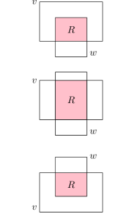
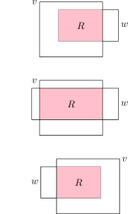
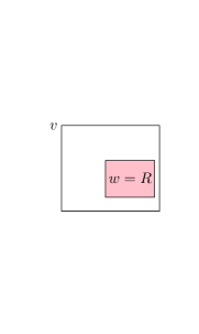
v-pairs	h-pairs	o-pair

Figure 2: Examples of v-pairs, h-pairs, and an o-pair.

Our proof works by finding a path in a rectangle intersection graph $G$ that defines a sequence of rectangles having properties that ensure that these rectangles form a clique.

See Figure 3 for an illustration of the following definition: Let $v_{1},\ldots,v_{k}$ be a sequence of rectangles and let $R_{i}=\bigcap_{j=1}^{i}v_{j}$. We say that $v_{1},\ldots,v_{k}$ is hvo-alternating if

1. for each $i\in\{2,\ldots,k\}$, $v_{i}\cap R_{i-1}\neq\emptyset$;

2. for each $i\in\{2,\ldots,k\}$, $v_{i}$ does not contain any corner of $R_{i-1}$; and

3. for each $i\in\{2,\ldots,k-1\}$, $(R_{i-1},v_{i})$ and $(R_{i},v_{i+1})$ are not both h-pairs and not both v-pairs.

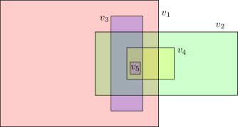
Figure 3: An hvo-alternating sequence of rectangles.

Note that Property 1 with $i=k$ ensures that $\bigcap_{j=1}^{k}v_{i}\neq\emptyset$. Therefore, if $v_{1},\ldots,v_{k}$ are vertices in a rectangle intersection graph $G$, then these vertices form a $k$-clique in $G$. Our proof attempts to grow an hvo-alternating sequence of vertices in $G$. The following lemma shows that an hvo-alternating sequence is neatly summarized by its last two elements:

Lemma 31.

If $v_{1},\ldots,v_{k}$ is an hvo-alternating sequence of rectangles then $\bigcap_{i=1}^{k}v_{i}=v_{k-1}\cap v_{k}$.

Proof.

The case $k=2$ is trivial, so we first consider the case $k=3$. Recall that, for any two sets $A$ and $B$, $A\supseteq B$ if and only if $A\cap B=B$. Therefore, it is sufficient to show that $v_{1}\supseteq v_{2}\cap v_{3}$.

If $(v_{1},v_{2})$ is an o-pair, then $v_{1}\supseteq v_{2}\supseteq v_{2}\cap v_{3}$ and we are done. Otherwise, assume without loss of generality that $(R_{1},v_{2})=(v_{1},v_{2})$ is an h-pair, so that $(R_{2},v_{3})$ is not an h-pair. Refer to Figure 4. In this case, $v_{2}\cap v_{3}$ is contained in the rectangle $R^{*}$ whose top and bottom sides coincide with those of $v_{2}$ and whose left and right sides coincide with those of $v_{1}$. We finish by Observing that $v_{1}\supseteq R^{*}\supseteq v_{2}\cap v_{3}$, as required.

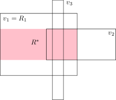
Figure 4: The proof of Lemma 31.

Next consider the general case $k>3$. By Lemma 31, the three element sequence $R_{k-2},v_{k-1},v_{k}$ is an hvo-alternating sequence so, applying the result for $k=3$, we obtain

$$\bigcap_{j=1}^{k}v_{j}=R_{k-2}\cap v_{k-1}\cap v_{k}=v_{k-1}\cap v_{k}\enspace.\qed$$

Sometimes the process of growing our hvo-alternating sequence stalls. The following lemma shows that, when this process stalls, we can at least replace the last element in the sequence.

Lemma 32.

Let $v_{1},\ldots,v_{k}$ be an hvo-alternating sequence of rectangles and define $R_{i}=\bigcap_{j=1}^{i}v_{i}$. Let $v$ be a rectangle such that

1. $v\cap R_{k}\neq\emptyset$;

2. $v$ contains no corner of $R_{k}$; and

3. $v_{1},\ldots,v_{k},v$ is not hvo-alternating.

Then $v_{1},\ldots,v_{k-1},v$ is hvo-alternating.

Proof.

Notice that $v_{1},\ldots,v_{k},v$ satisfies all the conditions to be hvo-alternating except that $(R_{k-1},v_{k})$ and $(R_{k},v)$ are both h-pairs or both v-pairs. Without loss of generality assume that they are both h-pairs.

It is sufficient to show that $(R_{k-1},v)$ is not a v-pair so that, by replacing $v_{k}$ with $v$ we are replacing the h-pair $(R_{k-1},v_{k})$ with an h-pair or an o-pair. But this is immediate, since $v$ intersects $R_{k}$ but does not intersect the top or bottom side of $R_{k}$. Therefore $v$ cannot intersect the top or bottom side of $R_{k-1}\supseteq R_{k}$, so $(R_{k-1},v)$ is not a v-pair. ∎

If our process repeatedly stalls, then the hvo-alternating sequence we are growing never gets any longer; we only repeatedly change the last element in the sequence. Next we describe the sequences of rectangles that appear during these repeated stalls and show that such sequences (if long enough) also determine large cliques in $G$.

A sequence $v_{1},\ldots,v_{k}$ of rectangles is h-nesting with respect to a rectangle $R$ if, for each $i\in\{1,\ldots,k\}$, $(R,v_{i})$ is an h-pair and, for each $i\in\{2,\ldots,k\}$, $(R\cap v_{i-1},v_{i})$ is an h-pair; see Figure 5. A v-nesting sequence is defined similarly by replacing h-pair with v-pair.

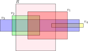
Figure 5: Rectangles $v_{1},\ldots,v_{4}$ that are h-nesting with respect to $R$.

Lemma 33.

If $v_{1},\ldots,v_{k}$ is an h-nesting sequence or a v-nesting sequence with respect to $R$, then there exists a point $x\in R$ such that $|\{i:x\in v_{i}\}|\geqslant\lceil k/2\rceil$.

Proof.

Assume, without loss of generality, that $v_{1},\ldots,v_{k}$ is an h-nesting sequence with respect to $R$. Consider the sequence of horizontal strips $s_{1},\ldots,s_{k}$, where each $s_{i}=(-\infty,\infty)\times(y_{i,1},y_{i,2})$ has top and bottom sides that coincide with those of $v_{i}$. Since, for each $i\in\{2,\ldots,k\}$, $(R,v_{i-1})$ and $(R\cap v_{i-1},v_{i})$ are both h-pairs, $s_{1}\supseteq s_{2}\supseteq\cdots\supseteq s_{k}$. Let $\ell$ be a point on the left side of $R$ contained in $s_{k}$ and let $r$ be a point on the right side of $R$ contained in $s_{k}$. Since $(R,v_{i})$ is an h-pair, $v_{i}$ contains at least one of $\ell$ or $r$, for each $i\in\{1,\ldots,k\}$. Therefore, at least one of $\ell$ or $r$ is contained in at least $\lceil k/2\rceil$ rectangles in $v_{1},\ldots,v_{k}$. Since rectangles are open, there is a point $x$, in the neighbourhood of $\ell$ or $r$ (as appropriate) that is contained in $R$ and is also contained in $\lceil k/2\rceil$ rectangles in $v_{1},\ldots,v_{k}$. ∎

We now introduce a particular 2-tree. The height-$h$ $d$-branching universal 2-tree, $T_{h,d}$ is defined recursively as follows:

• $T_{-1,d}$ is the empty graph;

• $T_{0,d}$ is a two-vertex graph with a single edge;

• For $h\geqslant 1$, $T_{h,d}$ is obtained from $T_{h-1,d}$ by adding, for each edge $vw\in E(T_{h-1,d})\setminus E(T_{h-2,d})$, $d$ new vertices $v_{1,vw},\ldots,v_{d,vw}$ each adjacent to both $v$ and $w$.

The root edge of $T_{h,d}$ is the single edge of $T_{0,d}$. For each $i\in\{0,\ldots,h\}$, the level-$i$ vertices of $T_{h,d}$ are the vertices in $V(T_{i,d})\setminus V(T_{i-1,d})$. The level-$i$ edges of $T$ are the edges that join a level-$i$ vertex to a level-$j$ vertex for some $j<i$.

Note that the number of level-$i$ edges in $T_{h,d}$ is given by the recurrence

$$m_{i}=\begin{cases}1&\text{if $i=0$}\\ 2dm_{i-1}&\text{otherwise}\end{cases}$$

which resolves to $(2d)^{i}$. Thus, the total number of edges in $T_{h,d}$ is less than $(2d)^{h+1}$.

We are now ready to prove the main result of this section.

Theorem 34.

For each $k\in\mathbb{N}$, every rectangle intersection graph that contains $T_{4k-7,(k-1)^{2}}$ as a subgraph contains a clique of size $k$.

Proof.

The cases $k=1$ and $k=2$ are trivial so, for the remainder of the proof we assume that $k\geqslant 3$.

Let $G$ be a rectangle intersection graph that contains $T=T_{4k-7,(k-1)^{2}}$ as a spanning subgraph. We use the convention that $V(G)=V(T)$ so that vertices of $T$ are rectangles in $V(G)$. We will attempt to define a path $v_{1},\ldots,v_{k}$ in $T$ such that $v_{1},\ldots,v_{k}$ is hvo-alternating.

Let $r_{0}r_{1}$ be the root edge of $T$. We set $v_{1}=r_{0}$ and use the convention that $v_{0}=r_{1}$. We will perform $(k-1)^{2}$ iterations, each of which tries to add another vertex, $v_{i+1}$, to a partially constructed hvo-alternating path $v_{1},\ldots,v_{i}$. During iteration $t$, for each $t\in\{1,\ldots,(k-1)^{2}\}$, the procedure will consider a level-$t$ vertex, $v$, of $T$ to include in the path. At the end of iteration $t$, the last vertex in the partially constructed sequence is always $v$, a level-$t$ vertex.

At the beginning of iteration $t$, $v_{i}$ is a level-$(t-1)$ vertex, so $v_{i-1}$ and $v_{i}$ are both adjacent to a set $S$ of $4k-7$ level-$t$ vertices. Each of the rectangles in $S$ intersects $v_{i-1}$ and $v_{i}$ so, by 30, each rectangle in $S$ intersects $v_{i-1}\cap v_{i}$. Therefore, by Lemma 31, each of the rectangles in $S$ intersects $R_{i}=\bigcap_{j=1}^{i}v_{j}$.

If each rectangle in $S$ contains at least one corner of $R_{i}$, then some corner of $R_{i}$ is contained in at least

$$\left\lceil(4k-7)/4\right\rceil=k-1$$

rectangles. Since these rectangles are open, there is a point $x$ contained in these $k-1$ rectangles and in $v_{i}$. The resulting set of $k$ rectangles therefore form a $k$-clique in $G$ and we are done.

Otherwise, some rectangle $v\in S$ does not contain a corner of $R_{i}$. Notice that the sequence $v_{1},\ldots,v_{i},v$ is hvo-alternating except, possibly, that the pairs $(R_{i-1},v_{i})$ and $(R_{i},v)$ are both h-pairs or both v-pairs. There are two cases to consider:

1. $v_{1},\ldots,v_{i},v$ is hvo-alternating. In this case we say that the procedure succeeds in iteration $t$ and we set $v_{i+1}=v$.

2. $v_{1},\ldots,v_{i},v$ is not hvo-alternating. In this case, we say that the procedure stalls in iteration $t$. In this case, we change $v_{i}$ by setting $v_{i}=v$. By Lemma 32 the resulting sequence is hvo-alternating,

   Note that in this case we have failed to make our path any longer. Instead, we have only replaced the last element with a level-$t$ vertex. Regardless, the next iteration will try to extend the path with the new value of $v_{i}$.

If we allow this procedure to run sufficiently long, then one of two cases occurs:

1. At least $k-1$ iterations are successes. In this case, we find $v_{2},\ldots,v_{k}$, so that $v_{1},\ldots,v_{k}$ is an hvo-sequence whose vertices form a $k$-clique in $G$.

2. Some element of our sequence, $v_{i}$ takes on a sequence $S_{i}=v_{i,0},\ldots,v_{i,2(k-i)}$ of $2(k-i)+1$ different values because the procedure stalls $2(k-i)$ times while trying to select $v_{i+1}$. In this case, $S_{i}$ is either h-nesting or v-nesting with respect to $R_{i-1}$ so, by Lemma 33, some subset $\{w_{0},\ldots,w_{k-i}\}\subset S_{i}$ of rectangles in $S_{i}$ all have a common intersection that includes a point of $R_{i-1}$. But $R_{i-1}$ is the common intersection of $v_{1},\ldots,v_{i-1}$. Therefore $v_{1},\ldots,v_{i-1},w_{0},\ldots,w_{k-i}$ all have a point in common and form a $k$-clique in $G$.

The number of iterations required before this procedure finds a $k$-clique in $G$ is at most

$$h=\sum_{i=2}^{k}(2(k-i)+1)=k+(k-2)(k+1)=(k-1)^{2}\enspace.$$

During these $h$ iterations, the procedure selects a level-$j$ vertex of $T$ for $j=1,2,\ldots,h$. Since $T$ has height $(k-1)^{2}=h$, the procedure succeeds in finding a $k$-clique before running out of levels. ∎

This completes the proof of Theorem 29.

We now give an application of Theorem 29 in the setting of graph partitions.

Proposition 35.

There is no constant $c$ such that every series-parallel graph has a vertex-partition into two induced subgraphs each with pathwidth at most $c$.

Proof.

Suppose that every series-parallel graph $G$ has such a partition $\{V_{1},V_{2}\}$ of $V(G)$, where $P_{1}$ and $P_{2}$ are path decompositions of $G[V_{1}]$ and $G[V_{2}]$ respectively, each with width at most $c$. Adding $V_{2}$ to every bag of $P_{1}$ and $V_{1}$ to every bag of $P_{2}$ gives two $(2c+2)$-orthogonal path decompositions of $G$, contradicting Theorem 29. ∎

This result is in contrast to a theorem of DeVos et al. [18], which says that for every fixed graph $H$ there is a constant $c$, such that every $H$-minor-free graph has a vertex-partition into two induced subgraphs each with treewidth at most $c$.

8 Boxicity Connections

Section 7 attempts to understand which graphs have two path decompositions with bounded intersections. This turns out to be equivalent to the more geometric problem of understanding which graphs are subgraphs of rectangle intersection graphs of bounded clique size. There are several other ways we could generalize these problems.

Does adding extra dimensions help? A $d$-dimensional box intersection graph is a graph whose vertices are $d$-dimensional axis-aligned boxes and for which two vertices are adjacent if and only if they intersect. For a graph, $G$, the smallest $d$ such that $G$ is a $d$-dimensional box intersection graph is known as the boxicity of $G$.

Open Problem 1.

For each $d\in\mathbb{N}$, what is the smallest value of $r=r_{d}$ for which the following statement is true: For every $k\in\mathbb{N}$ there exists an $r$-tree $T$ such that every graph $G$ of boxicity $d$ that contains $T$ as a subgraph contains a $k$-clique?

Theorem 34 shows that $r_{2}\leqslant 2$, and the obvious representation of trees (1-trees) as rectangle intersection graphs shows that $r_{2}>1$, so $r_{2}=2$. For $d>2$, we now show that $r_{d}\leqslant 2d$.

Proposition 36.

For every $k\geqslant 2$ and $d\geqslant 1$, there exists a $2d$-tree $T_{k}$ such that every intersection graph of $d$-dimensional boxes that contains $T_{k}$ as a subgraph contains a $k$-clique.

Proof.

The $2d$-tree $T_{k}$ is defined inductively: $T_{0}$ is a $(2d+1)$-clique. To obtain $T_{i}$, attach a vertex adjacent to each $2d$-clique in $T_{i-1}$.

Now consider some box representation of a graph $G$ that contains $T_{r}$ as a subgraph, so that the vertices of $G$ are $d$-dimensional boxes. We find the desired clique inductively by constructing two sequences of sets $S_{0},\dots,S_{r}$ and $X_{0}\subseteq\dots\subseteq X_{r}$ that satisfy the following conditions for each $i\in\{0,1,\dots,r\}$:

1. $|S_{i}|=2d$,

2. $S_{i}\subseteq X_{i}\subseteq V(T_{i})$,

3. $S_{i}$ forms a clique in $T_{i}$,

4. $\cap X_{i}=\cap S_{i}$ (so $X_{i}$ is a $(2d+1+i)$-clique in $G$).

Let $X_{0}:=V(T_{0})$. To find $S_{0}$, look at the common intersection $\cap X_{0}$. At least one of the boxes $x$ in $X_{0}$ is redundant in the sense that $\cap X_{0}=\cap(X_{0}\setminus{x})$. Let $S_{0}:=X_{0}\setminus\{x\}$. Observe that $X_{0}$ and $S_{0}$ satisfy Conditions 1–4.

Now for the inductive step. By Conditions 1 and 3, the vertices of $S_{i}$ form a $2d$-clique in $T_{i}$, so there is some vertex $v$ in $T_{i+1}$ that is adjacent to all the vertices in $S_{i}$. Let $X_{i+1}:=X_{i}\cup\{v\}$ and let $S_{i+1}$ be the subset of $S_{i}\cup\{v\}$ obtained by removing one redundant box. Then $X_{i+1}$ and $S_{i+1}$ satisfy Conditions 1–4.

Set $r:=\max\{0,k-2d-1\}$. Then every graph of boxicity at most $d$ that contains $T_{r}$ contains a $k$-clique. ∎

On the lower-bound side, a result of Thomassen [59] states that every planar graph has a boxicity at most 3. Since every 2-tree is planar, this implies $r_{d}\geqslant 3$ for $d\geqslant 3$. More generally, Chandran and Sivadasan [10] show that every graph $G$ has boxicity at most $\operatorname{tw}(G)+2$, so every $(d-2)$-tree has boxicity at most $d$. This implies that $r_{d}\geqslant d-1$.

Returning to two dimensions, recall that the Koebe–Andreev–Thurston theorem states that every planar graph is a subgraph of some intersection graph of disks for which no point in the plane is contained in more than two disks. 2-trees are a very special subclass of planar graphs, so Theorem 34 shows that axis-aligned rectangles are very different than disks in this respect. Thus, we might ask how expressive other classes of plane shapes are.

For a set $C$ of lines, we can consider intersection graphs of $C$-oriented convex shapes: convex bodies whose boundaries consist of linear pieces, each of which is parallel to some line in $C$. (Axis-aligned rectangles are $C$-oriented where $C$ is the set consisting of the x-axis and y-axis.) For a set $C$ of lines, let $\mathcal{G}_{C}$ denote the class of intersection graphs of $C$-oriented convex shapes. For an integer $c$, let $\mathcal{G}_{c}=\bigcup_{C:|C|=c}\mathcal{G}_{C}$.

Open Problem 2.

For each $c\in\mathbb{N}$, what is the smallest value of $r=r_{c}$ such that the following statement is true: For every $k\in\mathbb{N}$, there exists an $r$-tree $T$ such that every graph $G\in\mathcal{G}_{c}$ that contains $T$ as a subgraph contains a $k$-clique?

As in the proof of Proposition 36, we can use the fact that, for any set $B$ of $C$-oriented convex shapes, there is a subset $B^{\prime}\subset B$ with $|B^{\prime}|\leqslant 2|C|$ and $\cap B=\cap B^{\prime}$ to establish that $r_{c}\leqslant 2c$. We do not know a lower bound better than $r_{c}>1$.

9 Colouring Connections

The tree-chromatic number of a graph $G$, denoted by $\text{tree-}\chi(G)$, is the minimum integer $k$ such that $G$ has a tree decomposition in which each bag induces a $k$-colourable subgraph. This definition was introduced by Seymour [54]; also see [36, 4]. For a graph $G$, define the 2-dimensional treewidth of $G$, denoted $\operatorname{2-tw}(G)$, to be the minimum integer $k$ such that $G$ has two $k$-orthogonal tree decompositions $S$ and $T$. For each bag $B$ of $S$, note that $T$ defines a tree decomposition of $G[B]$ with width $k-1$, implying $G[B]$ is $k$-colourable. Thus

$$\operatorname{2-tw}(G)\geqslant\text{tree-}\chi(G)\geqslant\omega(G).$$ (3)

Obviously, $\operatorname{2-tw}(G)\geqslant\omega(G)$ and $\text{tree-}\chi(G)\geqslant\omega(G)$. Equation 3 leads to lower bounds on $\operatorname{2-tw}(G)$. For example, Seymour [54] showed that tree-chromatic number is unbounded on triangle-free graphs. Thus $\operatorname{2-tw}$ is also unbounded on triangle-free graphs.

On the other hand, we now show that there are graphs with bounded tree-chromatic number (even path-chromatic number) and unbounded $\operatorname{2-tw}$. The shift graph $H_{n}$ has vertex set $\{(i,j):1\leqslant i<j\leqslant n\}$ and edge set $\{(i,j)(j,\ell):1\leqslant i<j<\ell\leqslant n\}$. It is well known that $H_{n}$ is triangle-free with chromatic number at least $\log_{2}n$; see [35]. Seymour [54] constructed a path decomposition of $H_{n}$ such that each bag induces a bipartite subgraph. We prove the following result that separates $\text{tree-}\chi$ and $\operatorname{2-tw}$.

Theorem 37.

For every $k$ there exists $n$ such that the shift graph $H_{n}$ does not admit two $k$-orthogonal tree decompositions.

Lemma 38.

For every integer $\ell\geqslant 1$ there exists an even integer $m>\ell$ such that for every tree decomposition $T$ of the shift graph $H=H_{m}$,

(i)

$\chi(H[T_{x}])>\ell$ for some $x\in V(T)$, or

(ii)

there exists $x\in V(T)$, $A\subseteq\{1,2,\ldots,\frac{m}{2}\}$, and $B\subseteq\{\frac{m}{2}+1,\ldots,m\}$, such that $|A|,|B|>\ell$, and $(a,b)\in T_{x}$ for all $a\in A$ and $b\in B$.

Proof of Theorem 37 assuming Lemma 38..

Let $\ell=m(k)$, and let $n=m(\ell)$, where $m$ is as in Lemma 38. Then $n>\ell>k$. We show that $n$ satisfies the theorem. Suppose not, and let $T$ and $T^{\prime}$ be two $k$-orthogonal tree decompositions of $H_{n}$. Each bag $T_{x}$ induces a subgraph of treewidth at most $k-1$ in $H_{n}$. Thus $\chi(H[T_{x}])\leqslant k\leqslant\ell$. Thus outcome (i) of Lemma 38 applied to $\ell$ and $H$ does not hold for $T$, and so outcome (ii) holds. Let $x$, $A$ and $B$ be as in this outcome. We may assume that $|A|=|B|$. Let $H^{\prime}$ be the subgraph of $H$ induced by $\{(a,b)\in V(H):a,b\in A\cup B\}$. Then $H^{\prime}\cong H_{|A\cup B|}$. Apply Lemma 38 to $H^{\prime}$ and the tree decomposition $T^{\prime\prime}$ of $H^{\prime}$ induced by $T^{\prime}$. Each bag of $T^{\prime\prime}$ induces a $k$-colourable subgraph of $H^{\prime}$. Since $k<\ell$, outcome (ii) occurs. Thus there exist $A^{\prime}\subseteq A$ and $B^{\prime}\subseteq A$ and $x^{\prime}\in V(T^{\prime})$ such that $|A^{\prime}|,|B^{\prime}|\geqslant k+1$ and $(a,b)\in T^{\prime}_{x^{\prime}}$ for all $a\in A^{\prime}$ and $b\in B^{\prime}$. Thus $|T_{x}\cap T^{\prime}_{x^{\prime}}|\geqslant(k+1)^{2}>k$, yielding the desired contradiction. ∎

Proof of Lemma 38..

Define $m:=2^{4\ell+1}+2$. Let $T$ be a tree decomposition of the shift graph $H=H_{m}$. By splitting vertices of $T$, if necessary, we may assume that $T$ has maximum degree at most 3. Let $H^{1}$ be the subgraph of $H$ induced by pairs $(a,b)$ such that $a,b\leqslant\frac{m}{2}$, and let $H^{2}$ be the subgraph induced by pairs $(a,b)$ with $a,b>\frac{m}{2}$. Then $H^{1}\cong H^{2}\cong H_{m/2}$. For a subtree $X$ of $T$ and $i\in\{1,2\}$, let $H^{i}(X)$ denote the subgraph of $H^{i}$ induced by $V(H^{i})-\bigcup\{T_{x}:x\in V(T)\setminus V(X)\}$; that is, by those vertices of $H^{i}$ that only belong to the bags of $T$ corresponding to vertices of $X$. We may assume that (i) does not hold.

Suppose that there does not exist an edge $e\in E(T)$ such that $\chi(H^{1}(X))\geqslant\ell+1$ and $\chi(H^{1}(Y))\geqslant\ell+1$, where $X$ and $Y$ are the components of $T-e$. That is, $\chi(H^{1}(X))\leqslant\ell$ or $\chi(H^{1}(Y))\leqslant\ell$. Orient $e$ towards $X$ if $\chi(H^{1}(X))\leqslant\ell$ and towards $Y$ otherwise. Do this for every edge of $T$. Let $v$ be a source node in this orientation of $T$. Then $\chi(H^{1}(Z))\leqslant\ell$ for each subtree $Z$ of $T$ with $v\not\in V(Z)$. Let $Z_{1}$, $Z_{2}$ and $Z_{3}$ be the (at most) three maximal subtrees of $T-v$. Then $H^{1}(Z_{1})$, $H^{1}(Z_{2})$, $H^{1}(Z_{3})$ and $H^{1}[T_{v}]$ are four induced subgraphs of $H^{1}$ covering the vertex set of $H^{1}$, each with chromatic number at most $\ell$. Thus $\log_{2}\frac{m}{2}\leqslant\chi(H^{1})\leqslant 4\ell$, contradicting the choice of $m$.

Thus there exists an edge $e\in E(T)$ such that $\chi(H^{1}(X))\geqslant\ell+1$ and $\chi(H^{1}(Y))\geqslant\ell+1$, where $X$ and $Y$ are the components of $T-e$. Repeating the argument in the previous paragraph for $H^{2}$, we may assume without loss of generality that $\chi(H^{2}(Y))\geqslant\ell+1$. Let $A$ be the set of all $a$ such that $(b,a)\in V(H^{1}(X))$ for some $b<a$. Then $|A|\geqslant\ell+1$, since $H^{1}(X)$ can be properly coloured using one colour for each element of $A$. Similarly, if $B$ is the set of all $b$ such that $(b,a)\in V(H^{2}(Y))$ for some $a>b$, then $|B|\geqslant\ell+1$. Consider $(a,b)\in V(H)$ with $a\in A$ and $b\in B$. Then $(a,b)$ has a neighbour in $V(H^{1}(X))$ and therefore $(a,b)\in T_{x}$ for some $x\in V(X)$. Similarly, $(a,b)\in T_{y}$ for some $y\in V(Y)$. If $z$ is an endpoint of $e$, then $z$ lies on the $xy$-path in $T$, and thus $(a,b)\in T_{z}$ and (ii) holds. ∎

The above results suggest a positive answer to the following question.

Open Problem 3.

Is there a function $f$ such that every graph that has two $k$-orthogonal tree decompositions is $f(k)$-colourable? That is, is $\chi(G)\leqslant f(\operatorname{2-tw}(G))$ for every graph $G$?

This question asks whether graphs that have two tree decompositions with bounded intersections have bounded chromatic number. Note that graphs that have two path decompositions with bounded intersections have bounded chromatic number (since rectangle intersection graphs are $\chi$-bounded, as proved by Asplund and Grünbaum [2]). Also note that the converse to this question is false: there are 3-colourable graph classes with $\operatorname{2-tw}$ unbounded. Suppose the complete tripartite graph $K_{n,n,n}$ has two $k$-orthogonal tree decompositions. Then each decomposition has at least $2n+1$ vertices in some bag (since $\operatorname{tw}(K_{n,n,n})=2n$). The intersection of these two bags has size at least $n+2$. Thus $k\geqslant n+2$ and $\operatorname{2-tw}(K_{n,n,n})\geqslant n+2$.

Note.

Independently of this paper, Stavropoulos [56, 57] introduced the $i$-medianwidth of a graph for each $i\geqslant 1$. It is easily seen that $\operatorname{2-tw}(G)$ equals the 2-medianwidth of $G$. Following the initial release of this paper, Felsner et al. [27] answered 3 in the negative.

References

- Alon et al. [1990] Noga Alon, Paul Seymour, and Robin Thomas. A separator theorem for nonplanar graphs. J. Amer. Math. Soc., 3(4):801–808, 1990. doi: 10.2307/1990903. MR: 1065053.
- Asplund and Grünbaum [1960] Edgar Asplund and Branko Grünbaum. On a colouring problem. Math. Scand., 8:181–188, 1960.
- Bannister et al. [2015] Michael J. Bannister, William E. Devanny, Vida Dujmović, David Eppstein, and David R. Wood. Track layouts, layered path decompositions, and leveled planarity, 2015. arXiv: 1506.09145.
- Barrera-Cruz et al. [2017] Fidel Barrera-Cruz, Stefan Felsner, Tamás Mészáros, Piotr Micek, Heather Smith, Libby Taylor, and William T. Trotter. Separating tree-chromatic number from path-chromatic number. 2017. arXiv: 1703.03973.
- Bodlaender [1998] Hans L. Bodlaender. A partial -arboretum of graphs with bounded treewidth. Theoret. Comput. Sci., 209(1-2):1–45, 1998. doi: 10.1016/S0304-3975(97)00228-4.
- Bodlaender [1999] Hans L. Bodlaender. A note on domino treewidth. Discrete Math. Theor. Comput. Sci., 3(4):141–150, 1999. https://dmtcs.episciences.org/256. MR: 1691565.
- Bodlaender and Engelfriet [1997] Hans L. Bodlaender and Joost Engelfriet. Domino treewidth. J. Algorithms, 24(1):94–123, 1997. doi: 10.1006/jagm.1996.0854. MR: 1453952.
- Bollobás [1986] Béla Bollobás. Combinatorics: Set Systems, Hypergraphs, Families of Vectors, and Combinatorial Probability. Cambridge University Press, 1986.
- Bollobás and Duchet [1979] Béla Bollobás and Pierre Duchet. Helly families of maximal size. J. Comb. Theory, Ser. A, 26(2):197–200, 1979. doi: 10.1016/0097-3165(79)90071-2.
- Chandran and Sivadasan [2007] L. Sunil Chandran and Naveen Sivadasan. Boxicity and treewidth. J. Comb. Theory, Ser. B, 97(5):733–744, 2007. doi: 10.1016/j.jctb.2006.12.004.
- Chen [2001] Zhi-Zhong Chen. Approximation algorithms for independent sets in map graphs. J. Algorithms, 41(1):20–40, 2001. doi: 10.1006/jagm.2001.1178.
- Chen [2007] Zhi-Zhong Chen. New bounds on the edge number of a -map graph. J. Graph Theory, 55(4):267–290, 2007. doi: 10.1002/jgt.20237.
- Chen et al. [2002] Zhi-Zhong Chen, Michelangelo Grigni, and Christos H. Papadimitriou. Map graphs. J. ACM, 49(2):127–138, 2002. doi: 10.1145/506147.506148.
- Cygan et al. [2015] Marek Cygan, Fedor V. Fomin, Łukasz Kowalik, Daniel Lokshtanov, Dániel Marx, Marcin Pilipczuk, Michał Pilipczuk, and Saket Saurabh. Parameterized algorithms. Springer, 2015. doi: 10.1007/978-3-319-21275-3.
- Demaine et al. [0405] Erik D. Demaine, Fedor V. Fomin, MohammadTaghi Hajiaghayi, and Dimitrios M. Thilikos. Bidimensional parameters and local treewidth. SIAM J. Discrete Math., 18(3):501–511, 2004/05. doi: 10.1137/S0895480103433410. MR: 2134412.
- Demaine et al. [2005] Erik D. Demaine, Fedor V. Fomin, Mohammadtaghi Hajiaghayi, and Dimitrios M. Thilikos. Fixed-parameter algorithms for -center in planar graphs and map graphs. ACM Trans. Algorithms, 1(1):33–47, 2005. doi: 10.1145/1077464.1077468.
- Demaine and Hajiaghayi [2004] Erik D. Demaine and MohammadTaghi Hajiaghayi. Equivalence of local treewidth and linear local treewidth and its algorithmic applications. In Proc. 15th Annual ACM-SIAM Symposium on Discrete Algorithms (SODA ’04), pp. 840–849. SIAM, 2004. http://dl.acm.org/citation.cfm?id=982792.982919.
- DeVos et al. [2004] Matt DeVos, Guoli Ding, Bogdan Oporowski, Daniel P. Sanders, Bruce Reed, Paul Seymour, and Dirk Vertigan. Excluding any graph as a minor allows a low tree-width 2-coloring. J. Combin. Theory Ser. B, 91(1):25–41, 2004. doi: 10.1016/j.jctb.2003.09.001. MR: 2047529.
- Djidjev and Vrt’o [2003] Hristo N. Djidjev and Imrich Vrt’o. Crossing numbers and cutwidths. J. Graph Algorithms Appl., 7(3):245–251, 2003. doi: 10.7155/jgaa.00069.
- Dujmović et al. [2017] Vida Dujmović, David Eppstein, and David R. Wood. Structure of graphs with locally restricted crossings. SIAM J. Disc. Math., 31(2):805–824, 2017. doi: 10.1137/16M1062879. MR: 3639571.
- Dujmovic and Frati [2016] Vida Dujmovic and Fabrizio Frati. Stacks and queue layouts via layered separators. In Martin Nöllenburg and Yifan Hu, eds., Proc. 24th International Symposium on Graph Drawing and Network Visualization (GD ’16), vol. 9801 of Lecture Notes in Computer Science, pp. 511–518. Springer, 2016. arXiv: 1608.06458.
- Dujmović et al. [2017] Vida Dujmović, Pat Morin, and David R. Wood. Layered separators in minor-closed graph classes with applications. J. Combin. Theory Ser. B, 127:111–147, 2017. doi: 10.1016/j.jctb.2017.05.006. MR: 3704658.
- Dvořák and Norin [2014] Zdeněk Dvořák and Sergey Norin. Treewidth of graphs with balanced separations. 2014. arXiv: 1408.3869.
- Dvořák and Norin [2016] Zdeněk Dvořák and Sergey Norin. Strongly sublinear separators and polynomial expansion. SIAM J. Discrete Math., 30(2):1095–1101, 2016. doi: 10.1137/15M1017569.
- Eppstein [2000] David Eppstein. Diameter and treewidth in minor-closed graph families. Algorithmica, 27(3-4):275–291, 2000. doi: 10.1007/s004530010020. MR: 1759751.
- Fáry [1948] István Fáry. On straight line representation of planar graphs. Acta Univ. Szeged. Sect. Sci. Math., 11:229–233, 1948.
- Felsner et al. [2017] Stefan Felsner, Gwenaël Joret, Piotr Micek, William T. Trotter, and Veit Wiechert. Burling graphs, chromatic number, and orthogonal tree-decompositions. In Proc. Eurocomb 2017, vol. 61 of Electronic Notes in Discrete Math., pp. 415–420. 2017. doi: 10.1016/j.endm.2017.06.068. arXiv: 1703.07871.
- Fomin et al. [2012] Fedor V. Fomin, Daniel Lokshtanov, and Saket Saurabh. Bidimensionality and geometric graphs. In Proc. 23rd Annual ACM-SIAM Symposium on Discrete Algorithms, pp. 1563–1575. 2012. doi: 10.1137/1.9781611973099.124. arXiv: 1107.2221.
- Fox and Pach [2008] Jacob Fox and János Pach. Separator theorems and Turán-type results for planar intersection graphs. Adv. Math., 219(3):1070–1080, 2008. doi: 10.1016/j.aim.2008.06.002.
- Fox and Pach [2010] Jacob Fox and János Pach. A separator theorem for string graphs and its applications. Combin. Probab. Comput., 19(3):371–390, 2010. doi: 10.1017/S0963548309990459.
- Fox and Pach [2014] Jacob Fox and János Pach. Applications of a new separator theorem for string graphs. Combin. Probab. Comput., 23(1):66–74, 2014. doi: 10.1017/S0963548313000412.
- Grohe [2003] Martin Grohe. Local tree-width, excluded minors, and approximation algorithms. Combinatorica, 23(4):613–632, 2003. doi: 10.1007/s00493-003-0037-9. MR: 2046826.
- Grohe and Marx [2009] Martin Grohe and Dániel Marx. On tree width, bramble size, and expansion. J. Combin. Theory Ser. B, 99(1):218–228, 2009. doi: 10.1016/j.jctb.2008.06.004. MR: 2467827.
- Harvey and Wood [2017] Daniel J. Harvey and David R. Wood. Parameters tied to treewidth. J. Graph Theory, 84(4):364–385, 2017. doi: 10.1002/jgt.22030. MR: 3623383.
- Hell and Nešetřil [2004] Pavol Hell and Jaroslav Nešetřil. Graphs and homomorphisms. Oxford University Press, Oxford, 2004. doi: 10.1093/acprof:oso/9780198528173.001.0001.
- Huynh and Kim [2017] Tony Huynh and Ringi Kim. Tree-chromatic number is not equal to path-chromatic number. J. Graph Theory, 86(2):213–222, 2017. doi: 10.1002/jgt.22121. MR: 3684783.
- Joret and Wood [2013] Gwenaël Joret and David R. Wood. Complete graph minors and the graph minor structure theorem. J. Combin. Theory Ser. B, 103:61–74, 2013. doi: 10.1016/j.jctb.2012.09.001.
- Kawarabayashi and Reed [2010] Ken-ichi Kawarabayashi and Bruce Reed. A separator theorem in minor-closed classes. In Proc. 51st Annual Symposium on Foundations of Computer Science, FOCS ’10, pp. 153–162. IEEE, 2010. doi: 10.1109/FOCS.2010.22.
- Kratochvíl [1991] Jan Kratochvíl. String graphs. II. Recognizing string graphs is NP-hard. J. Combin. Theory Ser. B, 52(1):67–78, 1991. doi: 10.1016/0095-8956(91)90091-W.
- Lee [2016] James R. Lee. Separators in region intersection graphs. 2016. arXiv: 1608.01612.
- Matoušek [2014] Jiří Matoušek. Near-optimal separators in string graphs. Combin. Probab. Comput., 23(1):135–139, 2014. doi: 10.1017/S0963548313000400. MR: 3197972.
- Matoušek [2015] Jiří Matoušek. String graphs and separators. In Geometry, structure and randomness in combinatorics, vol. 18 of CRM Series, pp. 61–97. Ed. Norm., Pisa, 2015. MR: 3362300.
- Nešetřil and Ossona de Mendez [2012] Jaroslav Nešetřil and Patrice Ossona de Mendez. Sparsity, vol. 28 of Algorithms and Combinatorics. Springer, 2012. doi: 10.1007/978-3-642-27875-4. MR: 2920058.
- Norin [2015] Sergey Norin. New tools and results in graph minor structure theory. In Surveys in Combinatorics 2015, pp. 221–260. Cambridge University Press, 2015. doi: 10.1017/CBO9781316106853.008.
- Pach et al. [1996] János Pach, Farhad Shahrokhi, and Mario Szegedy. Applications of the crossing number. Algorithmica, 16(1):111–117, 1996. doi: 10.1007/BF02086610.
- Pach and Tóth [2002] János Pach and Géza Tóth. Recognizing string graphs is decidable. Discrete Comput. Geom., 28(4):593–606, 2002. doi: 10.1007/s00454-002-2891-4.
- Reed [1997] Bruce A. Reed. Tree width and tangles: a new connectivity measure and some applications. In Surveys in combinatorics, vol. 241 of London Math. Soc. Lecture Note Ser., pp. 87–162. Cambridge Univ. Press, 1997. doi: 10.1017/CBO9780511662119.006.
- Robertson and Seymour [2010] Neil Robertson and Paul Seymour. Graph minors I–XXIII. J. Combin. Theory Ser. B, 1983–2010.
- Robertson and Seymour [1986] Neil Robertson and Paul Seymour. Graph minors. II. Algorithmic aspects of tree-width. J. Algorithms, 7(3):309–322, 1986. doi: 10.1016/0196-6774(86)90023-4.
- Robertson and Seymour [2003] Neil Robertson and Paul Seymour. Graph minors. XVI. Excluding a non-planar graph. J. Combin. Theory Ser. B, 89(1):43–76, 2003. doi: 10.1016/S0095-8956(03)00042-X.
- Schaefer [2014] Marcus Schaefer. The graph crossing number and its variants: A survey. Electron. J. Combin., #DS21, 2014. http://www.combinatorics.org/DS21.
- Schaefer et al. [2003] Marcus Schaefer, Eric Sedgwick, and Daniel Štefankovič. Recognizing string graphs in NP. J. Comput. System Sci., 67(2):365–380, 2003. doi: 10.1016/S0022-0000(03)00045-X.
- Schaefer and Štefankovič [2004] Marcus Schaefer and Daniel Štefankovič. Decidability of string graphs. J. Comput. System Sci., 68(2):319–334, 2004. doi: 10.1016/j.jcss.2003.07.002.
- Seymour [2016] Paul Seymour. Tree-chromatic number. J. Combinat. Theory Series B, 116:229–237, 2016. doi: 10.1016/j.jctb.2015.08.002.
- Shahrokhi [2013] Farhad Shahrokhi. New representation results for planar graphs. In 29th European Workshop on Computational Geometry (EuroCG 2013), pp. 177–180. 2013. arXiv: 1502.06175.
- Stavropoulos [2015] Konstantinos Stavropoulos. On the medianwidth of graphs. 2015. arXiv: 1512.01104.
- Stavropoulos [2016] Konstantinos Stavropoulos. Cops, robber and medianwidth parameters. 2016. arXiv: 1603.06871.
- Syḱora and Vrt’o [1994] Ondrej Syḱora and Imrich Vrt’o. On VLSI layouts of the star graph and related networks. Integration VLSI J., 17 (1):83–93, 1994.
- Thomassen [1986] Carsten Thomassen. Interval representations of planar graphs. J. Comb. Theory, Ser. B, 40(1):9–20, 1986. doi: 10.1016/0095-8956(86)90061-4.
- Wood [2009] David R. Wood. On tree-partition-width. European J. Combin., 30(5):1245–1253, 2009. doi: 10.1016/j.ejc.2008.11.010. MR: 2514645.