Nucleon Charges from 2+1+1-flavor HISQ and 2+1-flavor clover lattices
Abstract:
Precise estimates of the nucleon charges , and are needed in many phenomenological analyses of SM and BSM physics. In this talk, we present results from two sets of calculations using clover fermions on 9 ensembles of 2+1+1-flavor HISQ and 4 ensembles of 2+1-flavor clover lattices. We show that high statistics can be obtained cost-effectively using the truncated solver method with bias correction and the coherent source sequential propagator technique. By performing simulations at 4–5 values of the source-sink separation , we demonstrate control over excited-state contamination using 2- and 3-state fits. Using the high-precision 2+1+1-flavor data, we perform a simultaneous fit in , and to obtain our final results for the charges.
1 Introduction
In this talk, we highlight three areas in which significant progress has been made to extract matrix elements of quark bilinear operators within nucleon states. (i) cost-effective increase of statistics using the truncated solver method with bias correction and the coherent source sequential propagator technique; (ii) inclusion of up to 4-states (3-states) in the analysis of 2-point (3-point) correlation functions; and (iii) a simultaneous fit in , and to data at different , and to get the physical value. The results presented here are based on Refs. [10, 3, 11]. A summary of the lattice ensembles used and measurements made in the clover-on-HISQ study is given in Table 1 and in the clover-on-clover study in Table 2. Associated results for the isovector form factors: , ,, and were presented by Yong-Chull Jang at this conference [8].
2 Increasing Statisitics Cost-effectively
The various systematic uncertainties in the calculation of matrix elements (ME) of local quark bilinear operators within nucleon states are at the 5% level [3]. In order to isolate, understand and address these systematics, one needs data with statistical errors that are significantly smaller. To reduce statistical errors, one needs to make measurements on significant numbers of decorrelated lattices that adequately importance sample the phase space of the path integral. We have found the following three techniques to be cost-effective ways of reducing the statistical errors.
Lattices with can be regarded as consisting of a large number of uncorrelated regions, i.e., measurements of nucleon correlation functions in different sub-regions are statistically uncorrelated. Since the generation of lattices with dynamical fermions is expensive, one should assess the dimensions of these sub-regions. For ME within nucleon states we find that measurements per lattice of size are cost-effective [10]. Furthermore, choosing the source points randomly within these sub-regions of a lattice and between lattices reduces correlations.
Computer time can be reduced significantly by using the coherent source sequential propagator method [10]. For example, if measurements on a given lattice are done in a single computer job, then the number of quark propagators that need to be calculated using coherent sources reduces to from in the standard approach.
Lastly, in a given measurement, one has the freedom to choose the precision with which quark propagators are calculated. The truncated solver method [1] with bias correction [5] significantly reduces the computational time. In Ref. [3], we show that a stopping residue reduces cost by a factor of about 17 compared to . Possible bias is corrected for using
where and are the 2- and 3-point correlation functions calculated in low- (LP) and high-precision (HP), respectively, and and are the two kinds of source positions. Bias, given by the second term, if present, was much smaller than the statistical errors. Speedup is achieved because we need 1 HP and LP measurement for bias correction for every 32 LP used for statisitcs.
| Ensemble ID | (fm) | (MeV) | (MeV) | |||||
| a12m310 | 0.1207(11) | 305.3(4) | 310(3) | 4.55 | 1013 | 8104 | 64832 | |
| a12m220S | 0.1202(12) | 218.1(4) | 225(2) | 3.29 | 1000 | 24000 | ||
| a12m220 | 0.1184(10) | 216.9(2) | 228(2) | 4.38 | 958 | 7664 | ||
| a12m220L | 0.1189(9) | 217.0(2) | 228(2) | 5.49 | 1010 | 8080 | 68680 | |
| a09m310 | 0.0888(8) | 312.7(6) | 313(3) | 4.51 | 881 | 7048 | ||
| a09m220 | 0.0872(7) | 220.3(2) | 226(2) | 4.79 | 890 | 7120 | ||
| a09m130 | 0.0871(6) | 128.2(1) | 138(1) | 3.90 | 883 | 7064 | 84768 | |
| a06m310 | 0.0582(4) | 319.3(5) | 320(2) | 4.52 | 1000 | 8000 | 64000 | |
| a06m220 | 0.0578(4) | 229.2(4) | 235(2) | 4.41 | 650 | 2600 | 41600 | |
| a06m135 | 0.0568(1) | 135.5(2) | 136(2) | 3.74 | 229 | 1145 | 36640 |
| Ensemble ID | (fm) | (MeV) | |||||
|---|---|---|---|---|---|---|---|
| a127m285 | 0.127(2) | 285(3) | 5.85 | 1000 | 4020 | 128480 | |
| a094m280 | 0.094(1) | 278(3) | 4.11 | 1005 | 3015 | 96480 | |
| a091m170 | 0.091(1) | 166(2) | 3.7 | 629 | 2516 | 80512 | |
| a091m170L | 0.091(1) | 172(6) | 5.08 | 467 | 2335 | 74720 |
3 Reducing Systematic Uncertainties
The above techniques allowed us to make, on each ensemble, measurements on lattices. In these measurements of 2- and 3-point correlation functions, two systematics need to be addressed in order to extract the charges, form factors, and other ME: removing excited-state contamination (ESC) and precise determination of the renormalization factor connecting the lattice operator to some phenomenological scheme such as the scheme at .
ESC arises because typical interpolating operators used to create and annihilate meson and baryon states on the lattice couple to the ground state, all its excitations and multiparticle states with the same quantum numbers. Thus, contributions of all higher states have to be removed to obtain the desired ME within the ground state. The behavior of the 2- and 3-point correlation functions, given by the spectral decomposition, has contributions from a tower of intermediate states in terms of unknown amplitudes , energies and ME that are extracted from fits. Formally, the ground state ME can be obtained by calculating the 3-point functions with very large source-sink separation . For baryons, the signal in 2- and 3-point function degrades exponentially, and for values of accessible with measurements, the ESC is found to be significant. Thus, methods to miminize ESC in calculations with fm are needed.
We demonstrate control over ESC by (i) constructing the interpolating operators using tuned smeared sources in the generation of the quark propagators; (ii) performing the calculation at multiple values of ; (iii) inserting the operator at all intermediate timeslices between the source and sink; (iv) analyzing the 2- and 3-point correlators by including increasing number of intermediate states. For example, the 2-state truncation of the zero-momentum correlation functions is
| (1) | ||||
| (2) |
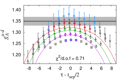
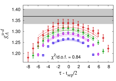
where is the operator insertion time and in the 3-point function calculation. The states and represent the ground and “first excited” nucleon states, respectively. In 2-state analysis, the four parameters, , , and are estimated first from fits to the 2-point data and then used as input in fits to 3-point functions to obtain the three ME , and . The estimate of the charge improves with number of , the precision of the data, and the number of states included in the fits. We find that with measurements, fits with 4 states (3 states) to the 2-point (3 point) functions with full covariance matrix can be made. Stable and consistent estimates of the charges in the limit are obtained using data with 4–5 values of in the range 1–1.5 fm. A comparison of the 2- and 3-state fits, and the consistency of the value obtained for the isovector axial charge is illustrated in Fig. 1.
Results for the various ME are then renormalized by multiplicative factors calculated using the RI-sMOM scheme as discussed in Ref. [3]. Errors in the ME and are combined in quadratures. This gives us a set of renomalized lattice estimates as functions of , and .

4 Simultaneous fit in , and
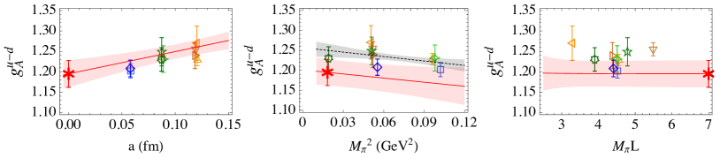
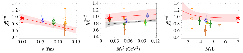
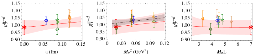
With the renormalized estimates, calculated as functions of , and , in hand, results in the limit , MeV and , are obtained using a simultaneous fit in the three variables. With the current 9 clover-on-HISQ data points, fits are sensitive to only the lowest order correction terms [3]:
| (3) | ||||
| (4) |
Adding next order terms such as chiral logs did not improve the fits (based on the Akaike Information Criteria) and their coefficients were poorly determined. Variation in estimates on including chiral logs were, nevertheless, used to obtain first estimates of the possible systematic uncertainty due to using the lowest order fit ansatz. Our final fits using Eqs. (3)and (4) are shown in Fig. 2.
The Clover-on-clover esimates on 4 ensembles are consistent with those from clover-on-HISQ at similar values of the lattice parameters. To perform analogous fits to obtain results at and MeV, clover-on-clover calculations are being extended to additional values of and .
5 Results: Nucleon Charges to quark EDM
(I) Our results for the isovector nucleon charges, using the simultaneous fit ansatz defined in Eqs. (3) and (4) to the 9 clover-on-HISQ data points, are shown in Fig. 2 and give [3]
| (5) |
(II) Using the conserved vector current relation , lattice estimates of given by FLAG [9], and our result for we obtain
| (6) |
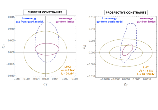
(III) Constraints on novel scalar and tensor couplings,
and , at the TeV scale using low-energy experiments and our
and are derived and compared with those
from the LHC in Fig. 3.
(IV) The leading opertors in a low-energy effective
theory that contribute to the neutron electric dipole moment (nEDM)
are the -term, the quark EDM operator and the quark chromo EDM
operators. The ME of the quark EDM operator, same as the flavor
diagonal tensor charges , are determined to be [2]
| (7) |
In these estimates, the disconnected contributions to and have been neglected as they were (smaller than the quoted errors) and poorly determined. Using these results and the experimental bound on the neutron EDM, we performed a first analysis of constraints on possible quark EDM couplings generated at the TeV scale and implications for a split SUSY model in Ref. [2, 4].
6 Conclusions and Outlook
Our goal is to calculate the charges and the form factors with uncertainty on each ensemble and obtain results in the , MeV limit with a total error of . This will require simulations with measurements at 4–5 values of the lattice spacing and on multiple values of the light quark masses close to the physical pion mass. To achieve this goal over the next 5–10 years will require further improvements in algorithms for generating lattices, physics analysis, and the calculation of renormalization factors. Work towards these three goals is ongoing.
Acknowledgments
We thank the MILC Collaboration for providing the 2+1+1-flavor HISQ ensembles and the JLab/W&M collaboration for the 2+1 clover lattices. Simulations were carried out on computer facilities of (i) Oak Ridge Leadership Computing Facility at the Oak Ridge National Laboratory, which is supported by the Office of Science of the U.S. Department of Energy under Contract No. DE-AC05-00OR22725; (ii) the USQCD Collaboration, which are funded by the Office of Science of the U.S. Department of Energy; (iii) the National Energy Research Scientific Computing Center, a DOE Office of Science User Facility supported by the Office of Science of the U.S. Department of Energy under Contract No. DE-AC02-05CH11231; and (iv) Institutional Computing at Los Alamos National Laboratory; and (v) the Extreme Science and Engineering Discovery Environment (XSEDE), which is supported by the NSF Grant No. ACI-1053575. The calculations used the Chroma software suite [6]. Work supported by the U.S. Department of Energy, NSF and the LANL LDRD program.
References
- [1] Gunnar S. Bali, Sara Collins, and Andreas Schafer. Effective noise reduction techniques for disconnected loops in Lattice QCD. Comput.Phys.Commun., 181:1570–1583, 2010.
- [2] T. Bhattacharya, V. Cirigliano, S. Cohen, R. Gupta, A. Joseph, H-W. Lin, and B. Yoon. Iso-vector and Iso-scalar Tensor Charges of the Nucleon from Lattice QCD. Phys. Rev., D92(9):094511, 2015.
- [3] T. Bhattacharya, V. Cirigliano, S. Cohen, R. Gupta, H-W. Lin, and B. Yoon. Axial, Scalar and Tensor Charges of the Nucleon from 2+1+1-flavor Lattice QCD. Phys. Rev., D94(5):054508, 2016.
- [4] T. Bhattacharya, V. Cirigliano, R. Gupta, H-W. Lin, and B. Yoon. Neutron Electric Dipole Moment and Tensor Charges from Lattice QCD. Phys. Rev. Lett., 115(21):212002, 2015.
- [5] Thomas Blum, Taku Izubuchi, and Eigo Shintani. New class of variance-reduction techniques using lattice symmetries. Phys.Rev., D88(9):094503, 2013.
- [6] Robert G. Edwards and Balint Joo. The Chroma software system for lattice QCD. Nucl.Phys.Proc.Suppl., 140:832, 2005.
- [7] P. Herczeg. Beta decay beyond the standard model. Prog. Part. Nucl. Phys., 46:413–457, 2001.
- [8] Y.C. Jang et al. ibid, 2016.
- [9] The Flavor Lattice Averaging Group (FLAG), 2016.
- [10] B. Yoon et al. Controlling Excited-State Contamination in Nucleon Matrix Elements. Phys. Rev., D93(11):114506, 2016.
- [11] B. Yoon et al. Isovector charges of the nucleon from 2+1-flavor QCD with clover fermions, 2016.