Fragmentation to a jet in the large $z$ limit

Abstract

We consider the fragmentation of a parton into a jet with small radius $R$ in the large $z$ limit, where $z$ is the ratio of the jet energy to the mother parton energy. In this region of phase space, large logarithms of both $R$ and $1-z$ can appear, requiring resummation in order to have a well defined perturbative expansion. Using soft-collinear effective theory, we study the fragmentation function to a jet (FFJ) in this endpoint region. We derive a factorization theorem for this object, separating collinear and collinear-soft modes. This allows for the resummation using renormalization group evolution of the logarithms $\ln R$ and $\ln(1-z)$ simultaneously. We show results valid to next-to-leading logarithmic order for the global Sudakov logarithms. We also discuss the possibility of non-global logarithms that should appear at two-loops and give an estimate of their size.

I Introduction

The fragmentation function (FF) Collins:1981uw , which describes an energetic splitting of a parton into a final state, is a very important ingredient in understanding high-energy hadron production. Using the FF we can systematically separate short- and long-distance interactions related to the production. For instance, inclusive hadron production for $e^{+}e^{-}$ annihilation can be factorized as

$$\frac{d\sigma(e^{+}e^{-}\to hX)}{dE_{h}}=\int^{1}_{z_{h}}\frac{dz}{z}\frac{d\sigma_{i}(z_{h}/z,\mu)}{dE_{i}}D_{h/i}(z,\mu),$$ (1)

where $i$ denotes the flavor of the produced parton, $z_{h}=2E_{h}/E_{cm}$, and $z=E_{h}/E_{i}$. Here, $E_{cm}$ is the center of the mass energy of the collision. The partonic scattering cross section $\sigma_{i}$ includes the hard interactions for $e^{+}e^{-}\to iX$. Long-distance interactions describing the fragmenting process from parton $i$ to hadron $h$ are encoded in the FF, $D_{h/i}(z)$. The FF is universal in the sense that it is independent of the hard process and can be applied to other scattering processes. Hence, the FF has long been studied in order to understand its properties. (For details we refer to a recent review Metz:2016swz and the references therein.)

Because we can directly observe a jet using well-defined jet algorithms such as the ones introduced in Refs. Catani:1993hr ; Ellis:1993tq ; Dokshitzer:1997in ; Salam:2007xv ; Cacciari:2008gp , it is possible to describe the fragmentation function to a jet (FFJ), as long as the the jet radius, $R$, is enough small Dasgupta:2014yra . (For a recent review of jet physics see, for example, Sapeta:2015gee .) Moreover, once the FFJ for the isolated jet is given, we can systematically investigate its substructures (e.g. hadron and subjet fragmentations Procura:2011aq ; Baumgart:2014upa ; Kaufmann:2015hma ; Chien:2015ctp ; Dai:2016hzf ; Kang:2016ehg , and jet mass Idilbi:2016hoa and transverse momentum Bain:2016rrv ; Neill:2016vbi distributions), constructing factorization theorems in connection with the frgmenting jet functions Procura:2009vm ; Jain:2011xz ; Ritzmann:2014mka .

Analytical results of the FFJ have been calculated up to the next-to-leading order (NLO) in $\alpha_{s}$ Kaufmann:2015hma ; Kang:2016mcy ; Dai:2016hzf . Unlike the hadron FF, the FFJ does not have any infrared (IR) divergence due to the finite size of the jet radius $R$. However, the presence of large logarithms of $R$ does not give a reliable result in perturbation theory and requires resummation to all order in $\alpha_{s}$. As shown in Refs. Dasgupta:2014yra ; Kaufmann:2015hma ; Kang:2016mcy ; Dai:2016hzf , resumming logarithms of $R$ is equivalent to running down to a scale $\mu\sim QR$ using Dokshitzer-Gribov-Lipatov-Altarelli-Parisi (DGLAP) evolution equations, where $Q$ is a hard energy comparable to the jet energy, $E_{J}$. This resummed result of the FFJ has been successfully applied to inclusive jet Kang:2016mcy ; Dasgupta:2016bnd and hadron Kang:2016ehg production, where the effects of various values of $R$ have been investigated in detail.

If we observe a highly energetic jet, we would expect that most of the energetic splitting processes are captured within the jet radius $R$ since these processes favor small angle radiation. This implies that the large $z$ region gives the dominant contribution to the FFJ, where $z$ is the ratio of the jet energy fraction over the mother parton energy. Accordingly, in the perturbative result for the FFJ there are large logarithms of $1-z$, which need to be resummed to all order in $\alpha_{s}$. Already at one loop order there appears a double logarithm $\ln(1-z)/(1-z)_{+}\sim L^{2}$, where $L$ schematic represents a large logarithm. At leading logarithm (LL) accuracy, the resummed can be represented as $\sum_{k=0}C_{k}(\alpha_{s}L^{2})^{k}\sim\exp(Lf_{0}(\alpha_{s}L))$, which gives the dominant correction to the perturbative expansion of the FFJ.

Thus, for a proper description of the FFJ in the large $z$ limit, we have to systematically handle large logarithms of $1-z$ as well as large logarithms of $R$. In general, if some quantity involves several distinct scales, we try to factorize it so that each factorized part can be well described at one properly chosen scale. Then performing evolutions between these largely separated scales, we resum the large logarithms. For the FFJ, soft-collinear effective theory (SCET) Bauer:2000ew ; Bauer:2000yr ; Bauer:2001yt ; Bauer:2002nz provides the appropriate framework for factorization and enable us to resum large logarithms automatically by solving the renormalization group (RG) equations for the factorized parts.

Near the endpoint where $z\to 1$, the FFJ consists of dynamics with two well-separated scales. Since an observed jet carries most of energy of the mother parton, radiation outside the jet should be soft with energy $\sim E_{J}(1-z)$. Therefore the jet splitting process can be initiated by soft dynamics, while radiation inside the jet is described dominantly by collinear interactions. However, in the effective theory approach wide angle soft interactions are not adequate for explaining the radiation outside the narrow jet because they cannot effectively recognize the jet boundary characterized by the small radius $R$. Instead, we introduce a more refined soft mode, namely the collinear-soft mode Bauer:2011uc ; Procura:2014cba , which can resolve the narrow jet boundary and can consistently describe the lower energy, out-of-jet radiations. The collinear-soft mode has previously been used to factorize the cross sections for a narrow jet at a low energy scale Becher:2015hka ; Chien:2015cka ; Becher:2016mmh ; Kolodrubetz:2016dzb .

In this paper, using SCET we construct a factorization theorem for the FFJ near the endpoint considering collinear and collinear-soft interactions. Then we resum the large logarithms of $1-z$ and $R$ simultaneously. In sec. II we discuss the characteristics of large-$z$ physics for the FFJ and factorize it into the collinear and the collinear-soft pieces. Then, we confirm our factorized result through NLO by an explicit calculation of each factorized part. In sec. III, based on the factorization, we resum the large logarithms by performing RG evolution. We also discuss large nonglobal logarithms (NGLs) that possibly contribute to NLL accuracy. In sec. IV the numerical results of the FFJ to the accuracy of NLL plus NLO in $\alpha_{s}$ are shown. Finally in sec. V we conclude.

II The FFJ in the limit $z\to 1$

Using SCET, the FFJ can be defined as Dai:2016hzf

$$D_{J_{k}/q}(z,\mu) = \sum_{X_{\notin J},X_{J-1}}\frac{z^{D-3}}{2N_{c}}\mathrm{Tr}\langle 0|\delta\Bigl{(}\frac{p_{J}^{+}}{z}-\mathcal{P}_{+}\Bigr{)}\frac{{\overline{n}}\!\!\!/}{2}\Psi_{n}|J_{k}(p_{J}^{+},R)X_{\notin J}\rangle\langle J_{k}(p_{J}^{+},R)X_{\notin J}|\bar{\Psi}_{n}|0\rangle,$$ (2)

$$D_{J_{k}/g}(z,\mu) = \sum_{X_{\notin J},X_{J-1}}\frac{z^{D-3}}{p_{J}^{+}(D-2)(N_{c}^{2}-1)}$$

$$\times\mathrm{Tr}\langle 0|\delta\Bigl{(}\frac{p_{J}^{+}}{z}-\mathcal{P}_{+}\Bigr{)}\mathcal{B}_{n}^{\perp\mu,a}|J_{k}(p_{J}^{+},R)X_{\notin J}\rangle\langle J_{k}(p_{J}^{+},R)X_{\notin J}|\mathcal{B}_{n\mu}^{\perp a}|0\rangle_{.}$$

Here $\Psi_{n}=W_{n}^{\dagger}\xi_{n}$ and $\mathcal{B}_{n}^{\perp\mu,a}=i\overline{n}^{\rho}g_{\perp}^{\mu\nu}G_{n,\rho\nu}^{b}\mathcal{W}_{n}^{ba}=i\overline{n}^{\rho}g_{\perp}^{\mu\nu}\mathcal{W}_{n}^{\dagger,ba}G_{n,\rho\nu}^{b}$ are gauge invariant collinear quark and gluon field strength respectively. $W_{n}$ ($\mathcal{W}_{n}$) is a collinear Wilson line in the fundamental (adjoint) representation Bauer:2000yr ; Bauer:2001yt . These collinear fields have momentum scaling $p_{n}^{\mu}=(p_{+},p_{\perp},p_{-})=Q(1,\lambda,\lambda^{2})$, where $\lambda$ is a small parameter comparable to small jet radius $R$. $p_{\pm}$ are denoted as $p_{+}\equiv\overline{n}\cdot p=p_{0}+\hat{{\bf{n}}}_{J}\cdot{\bf{p}}$ and $p_{-}\equiv n\cdot p=p_{0}-\hat{{\bf{n}}}_{J}\cdot{\bf{p}}$, where $\hat{{\bf{n}}}_{J}$ is a unit vector in the jet direction and two lightcone vectors $n^{\mu}=(1,\hat{{\bf{n}}}_{J})$ and $\overline{n}^{\mu}=(1,-\hat{{\bf{n}}}_{J})$ have been employed. The expressions for the FFJs in Eqs. (2) and (II) are valid in the jet frame where the transverse momentum of the observed jet, ${\bf{p}}^{\perp}_{J}$, is zero.

In this paper, we will consider inclusive $\mathrm{k_{T}}$-type algorithms Catani:1993hr ; Ellis:1993tq ; Dokshitzer:1997in ; Cacciari:2008gp , where the merging condition of two light particles is given by

$$\theta<R^{\prime}.$$ (4)

Here $\theta$ is the angle between the two particles, and $R^{\prime}=R$ for an $e^{+}e^{-}$ collider and $R^{\prime}=R/\cosh y$ for a hadron collider, where $y\sim\mathcal{O}(1)$ is the rapidity for the central region.

The definitions of the FFJs in Eqs. (2) and (II) hold for $z\sim\mathcal{O}(1)$, but are not reliable near the endpoint where $z$ goes to 1. In the limit $z\to 1$, the observed jet takes most of the energy from the mother parton and hence the jet splitting (out-jet) contributions should be described by soft gluon radiation. If $1-z$ is power counted as $\mathcal{O}(\eta)$ with $\eta\ll 1$, the relevant soft mode would have momentum scaling $k\sim(k_{+},k_{\perp},k_{-})\sim Q(\eta,\eta,\eta)$. However, for the proper resummation of $\ln R$, we need a mode that can probe the jet boundary expressed in terms of $R$. This mode would have a lower resolution than the soft mode while the $k_{+}$ component should still be power counted as $\mathcal{O}(\eta)$. Because the jet merging criterion for the soft gluon radiation is given by Ellis:2010rwa

$$\tan^{2}\frac{R^{\prime}}{2}>\frac{k_{-}}{k_{+}}\ ,$$ (5)

the proper mode should allow for the hierarchy, $k_{-}\sim k_{+}\lambda^{2}\ll k_{+}$, where $\lambda\sim R$. Thus this mode should have scaling $k\sim Q\eta(1,\lambda,\lambda^{2})$. From now on we will call this mode the collinear-soft mode.

We can consistently separate the usual soft mode $\sim Q(\eta,\eta,\eta)$ and the collinear-soft mode as was first done in the di-jet scattering cross section Becher:2015hka ; Chien:2015cka . Furthermore, the separation of the collinear-soft mode from the collinear fields has been performed in the formulation of $\mathrm{SCET_{+}}$ Bauer:2011uc . Because the collinear-soft mode can be considered as a subset of the usual soft mode, we have to subtract the overlapped of the collinear-soft contribution from the soft contribution in loop calculations similar to the usual zero-bin subtractions Manohar:2006nz .

If we apply this process to the FFJ with $z\to 1$, we see that the soft contributions can be cancelled by the collinear-soft subtractions. Since the soft mode with a scaling $(k_{+},k_{-})\sim Q(\eta,\eta)$ cannot resolve the jet boundary in Eq. (5), the real soft gluon radiation does not contribute to the in-jet contribution of the FFJ, while the out-jet contribution from real radiation covers the full phase space of $(k_{+},k_{-})$. Thus, independent of $R$, the total soft contributions will be expressed as a function of $1-z$, namely $S(1-z)$. For the collinear-soft contribution that needs to be subtracted from the soft contribution, we apply the same boundary conditions used for the soft mode. Hence the real collinear-soft radiation have only the out-jet contributions, which are the same as the soft mode. Therefore the net result of the collinear-soft contributions that are to be subtracted are the same as $S(1-z)$, canceling the soft contribution.

Finally we are left with a collinear-soft mode at the lower energy scale. When we apply this to the FFJ, we have to keep the jet boundary constraint in Eq. (5). As a result the active collinear-soft contributions can be expressed in terms of $1-z$ and $R$ simultaneously. As we will see, the one loop collinear-soft contributions involve double logarithms of $\ln\mu/((1-z)E_{J}R^{\prime})$. This fact indicates that the collinear-soft interactions are responsible for large logarithms of $1-z$ and its resummation would give the dominant contribution to the FFJ near the endpoint.

II.1 Factorization of the FFJ when $z\to 1$

With the above reasoning, we can systematically extend the FFJs to the endpoint region including collinear-soft interactions. We first decouple the soft mode $\sim Q(\eta,\eta,\eta)$ from the collinear mode $\sim Q(1,R,R^{2})$. Then we introduce the collinear-soft mode $\sim Q\eta(1,R,R^{2})$ in the collinear sector, classifying collinear and collinear-soft gluons as $A_{n}^{\mu}\to A_{n}^{\mu}+A_{n,cs}^{\mu}$. Accordingly the covariant derivative in the collinear sector decomposes as $iD^{\mu}=iD_{c}^{\mu}+iD_{cs}^{\mu}=\mathcal{P}^{\mu}+gA_{n}^{\mu}+i\partial^{\mu}+gA_{n,cs}^{\mu}$, where $\mathcal{P}^{\mu}~{}(i\partial^{\mu})$ returns collinear (collinear-soft) momentum. In this decomposition, the commutation relations, $[\mathcal{P}^{\mu},A_{n,cs}^{\nu}]=[\mathcal{\partial}^{\mu},A_{n}^{\nu}]=0$, hold. For the factorization of the FFJ, our strategy is simple: after the decomposition into the collinear and collinear-soft modes, we first integrate out collinear interactions with $p_{c}^{2}\sim Q^{2}R^{2}$. As we shall see, this gives an integrated jet function inside a jet. Then at the lower scale $\mu_{cs}\sim Q\eta R$ we will consider the collinear-soft interactions for the jet splitting.

As performed in Ref. Bauer:2011uc , at low energy we can additionally introduce so called ‘ultra-collinear’ modes after integrating out the collinear interactions with offshellness $p_{c}^{2}\sim Q^{2}R^{2}$. These modes have energy of the same order as the collinear mode, but their fluctuations are much smaller than $Q^{2}R^{2}$. Then at the low energy scale an external collinear field $\phi(=\xi,A)_{n}$ would be matched onto the ultra-collinear fields, $\phi_{n}=\phi_{n_{1}}+\phi_{n_{2}}+\cdots$, where the lightcone vectors $n_{i=1,2,\cdots}$ reside inside the jet with radius $R$. Note that collinear interactions between different ultra-collinear modes are forbidden since we have already integrated out the large collinear fluctuations $\sim Q^{2}R^{2}$. Moreover, as these ultra-collinear modes reside within the collinear interactions, they cannot resolve the jet boundary. Therefore their interactions do not contribute to the FFJs, at least to NLO in $\alpha_{s}$. So for simplicity we will not consider ultra-collinear interactions in the FFJ. However, in a more refined jet observable identifying subjets, these modes may have to be included.

Adding the collinear-soft mode, the quark initiated FFJ can be more generically expressed as

$$D_{J_{k}/q}(z,\mu)=\sum_{X_{\notin J},X_{J-1}}\frac{z^{D-3}}{2N_{c}}\mathrm{Tr}\langle 0|\delta\Bigl{(}\frac{p_{J}^{+}}{z}-\overline{n}\cdot iD\Bigr{)}\frac{{\overline{n}}\!\!\!/}{2}\xi_{n}|J_{k}(p_{J}^{+},R)X_{\notin J}\rangle\langle J_{k}(p_{J}^{+},R)X_{\notin J}|\bar{\xi}_{n}|0\rangle.$$ (6)

Compared to Eq. (2), $W_{n}\delta(p_{J}^{+}/z-\mathcal{P}_{+})W_{n}^{\dagger}=\delta(p_{J}^{+}/z-\overline{n}\cdot iD_{c})$ has been replaced with $\delta(p_{J}^{+}/z-\overline{n}\cdot iD)$ in Eq. (6).

In order to satisfy gauge invariances at each order in $\lambda\sim\mathcal{O}(R)$ and $\eta$, following the procedure considered in Ref. Bauer:2003mga , we redefine the collinear gluon field,

$$A_{n}^{\mu}=\hat{A}_{n}^{\mu}+\hat{W}_{n}[iD_{cs}^{\mu},\hat{W}_{n}^{\dagger}]_{,}$$ (7)

where $\hat{A}_{n}$ are newly defined collinear gluon fields and $\hat{W}_{n}$ is the collinear Wilson line expressed in terms of $\hat{A}_{n}$. As a consequence the covariant derivative in Eq. (6) can be rewritten as

$$iD^{\mu}=iD_{c}^{\mu}+W_{n}iD_{cs}^{\mu}W_{n}^{\dagger},$$ (8)

where collinear fields on the right-hand side are the redefined fields and we removed the hat for simplicity. Employing Eq. (8), the delta function in Eq. (6) can be rewritten as

$$\delta\Bigl{(}\frac{p_{J}^{+}}{z}-\overline{n}\cdot iD\Bigr{)}=W_{n}\delta\Bigl{(}\frac{p_{J}^{+}}{z}-\mathcal{P}_{+}-\overline{n}\cdot iD_{cs}\Bigr{)}W^{\dagger}_{n~{}.}$$ (9)

Similar to the decoupling of leading ultrasoft interactions from collinear fields Bauer:2001yt , we can remove collinear-soft interactions through the term $gn\cdot A_{cs}$ in the Lagrangian of the collinear sector. To accomplish this, the collinear quark and gluon fields can be additionally redefined as

$$\xi_{n}\to Y_{n}^{cs}\xi_{n},~{}~{}~{}A_{n}^{\mu}\to Y_{n}^{cs}A_{n}^{\mu}Y_{n}^{cs\dagger},$$ (10)

where $Y_{n}^{cs}$ is the collinear-soft Wilson line that satisfies $n\cdot iD_{cs}Y_{n}^{cs}=Y_{n}^{cs}n\cdot i\partial$ and has the usual form Bauer:2001yt ; Chay:2004zn

$$Y_{n}^{cs}(x)=\mathrm{P}~{}\exp\Biggl{[}ig\int^{\infty}_{x}dsn\cdot A_{cs}(sn)\Biggr{]}\ .$$ (11)

Using Eqs. (8) and (10) we rewrite Eq. (6) as

$$D_{J_{k}/q}(z,\mu) = \sum_{X_{\notin J},X_{J-1}}\frac{z^{D-3}}{2N_{c}}\mathrm{Tr}\langle 0|\delta\Bigl{(}\frac{p_{J}^{+}}{z}-\mathcal{P}_{+}-i\partial_{+}\Bigr{)}\frac{{\overline{n}}\!\!\!/}{2}Y_{\overline{n}}^{cs\dagger}Y_{n}^{cs}W_{n}^{\dagger}\xi_{n}|J_{k}(p_{J}^{+},R)X_{\notin J}\rangle$$ (12)

$$\qquad\times\langle J_{k}(p_{J}^{+},R)X_{\notin J}|\bar{\xi}_{n}W_{n}Y_{n}^{cs\dagger}Y_{\overline{n}}^{cs}|0\rangle_{,}$$

where we used the relation $\overline{n}\cdot iD_{cs}=Y_{\overline{n}}^{cs}i\partial_{+}Y_{\overline{n}}^{cs\dagger}$ and $Y_{\overline{n}}^{cs}$ has the same form as Eq. (11) with replacement of $n\to\overline{n}$. We also used the crossing symmetry $\phi\cdots|X_{\phi}\rangle=\langle X_{\phi}|\cdots\phi$, where $\phi=W_{n},~{}Y_{\overline{n}}^{cs}$. The FFJ in Eq. (12) can describe regions of ordinary $z\sim{\cal O}(1)$ and $z\to 1$. If $z$ is ordinary and not too close to 1, we can suppress $i\partial_{+}$ in the argument of the delta function, since $p_{J}^{+}/z-\mathcal{P}_{+}\sim\mathcal{O}(Q)$ is power counted much larger than $i\partial_{+}\sim\mathcal{O}(Q\eta)$. Thus the collinear-soft Wilson lines cancel by unitarity and we recover the form in Eq. (2). However, when $z\to 1$, $p_{J}^{+}/z-\mathcal{P}_{+}$ becomes the same size as $i\partial_{+}$, and we cannot ignore the term $i\partial_{+}$ in the delta function, which gives nonzero contributions of collinear-soft interactions.

Since $\mathcal{P}_{+}$ returns collinear (label) momentum in Eq. (12), $\mathcal{P}_{+}$ can be fixed as $p_{J}^{+}$ near the endpoint. Further, it means that collinear interactions are relevant only for jet merging (in-jet) contribution to the FFJ. Therefore the FFJ in the limit $z\to 1$ can be expressed as

$$D_{J_{q}/q}(z\to 1,\mu) = \sum_{X_{\notin J},X_{J-1}}\frac{z^{D-3}}{2N_{c}}\mathrm{Tr}\langle 0|Y_{\overline{n}}^{cs\dagger}Y_{n}^{cs}\frac{{\overline{n}}\!\!\!/}{2}W_{n}^{\dagger}\xi_{n}|J_{q}(p_{J}^{+},R)X_{\notin J}\rangle$$ (13)

$$\qquad\times\langle J_{q}(p_{J}^{+},R)X_{\notin J}|\bar{\xi}_{n}W_{n}\delta\Bigl{(}\frac{p_{J}^{+}}{z}-\mathcal{P}_{+}^{\dagger}+i\partial_{+}\Bigr{)}Y_{n}^{cs\dagger}Y_{\overline{n}}^{cs}|0\rangle$$

$$= \sum_{X_{c}\in J}\frac{1}{2N_{c}}\mathrm{Tr}\langle 0|\frac{{\overline{n}}\!\!\!/}{2}W_{n}^{\dagger}\xi_{n}|qX_{c}\in J\rangle\langle qX_{c}\in J|\bar{\xi}_{n}W_{n}|0\rangle\cdot\sum_{X_{cs}}\frac{1}{N_{c}}\mathrm{Tr}\langle 0|Y_{\overline{n}}^{cs\dagger}Y_{n}^{cs}|X_{cs}\rangle$$

$$\qquad\times\langle X_{cs}|\delta\bigl{(}(1-z)p_{J}^{+}+\Theta(\theta-R^{\prime})i\partial_{+}\bigr{)}Y_{n}^{cs\dagger}Y_{\overline{n}}^{cs}|0\rangle_{,}$$

where $\Theta$ is the step function and we reorganized the final states into collinear states $(qX_{c})$ in the jet and collinear-soft states $X_{cs}$ in order to factorize collinear and collinear-soft interactions. In the second equality we fixed the collinear label momentum $\mathcal{P}^{\dagger}$ as $p_{J}^{+}$, and then we put the jet splitting constraint in front of $i\partial_{+}$ because only the out-jet collinear-soft radiation gives a nonzero contribution for the region $z<1$. From Eq. (5), the jet splitting constraint $\Theta(\theta-R^{\prime})$ is equivalent to $\tan^{2}R^{\prime}/2<k_{-}/k_{+}$, where $k$ is the collinear-soft momentum.

Eq. (13) shows that the quark FFJ in the limit $z\to 1$ is factorized as

$$D_{J_{q}/q}(z\to 1,\mu;E_{J}R^{\prime},(1-z)E_{J}R^{\prime})=\mathcal{J}_{q}(\mu;E_{J}R^{\prime},\theta<R^{\prime})\cdot S_{q}(z,\mu;(1-z)E_{J}R^{\prime}),$$ (14)

where $\mathcal{J}_{q}$ is the integrated jet function for the in-jet contribution, defined as

$$\mathcal{J}_{q}(\mu;E_{J}R^{\prime},\theta<R^{\prime})=\sum_{X_{c}\in J}\frac{1}{2N_{c}~{}p_{J}^{+}}\mathrm{Tr}\langle 0|\frac{{\overline{n}}\!\!\!/}{2}W_{n}^{\dagger}\xi_{n}|qX_{c}\in J(E_{J},R^{\prime})\rangle\langle qX_{c}\in J|\bar{\xi}_{n}W_{n}|0\rangle_{.}$$ (15)

$S_{q}$ is the dimensionless collinear-soft function. When we rewrite $S_{q}=p_{J}^{+}\tilde{S}_{q}$, the dimensionful collinear-soft function $\tilde{S}_{q}$ can be expressed as

$$\tilde{S}_{q}(\ell_{+},\mu;\ell_{+}t)=\sum_{X_{cs}}\frac{1}{N_{c}}\mathrm{Tr}\langle 0|Y_{\overline{n}}^{cs\dagger}Y_{n}^{cs}|X_{cs}\rangle\langle X_{cs}|\delta\bigl{(}\ell_{+}+\Theta(\theta-R^{\prime})i\partial_{+}\bigr{)}Y_{n}^{cs\dagger}Y_{\overline{n}}^{cs}|0\rangle_{,}$$ (16)

where $t\equiv\tan R^{\prime}/2$, and $\ell_{+}t$ is the scale that will minimize large logarithms in the higher order corrections, as we will see later.

Using the adjoint representation and taking a similar procedure as we did with the quark case, we obtain the factorization formula for the gluon FFJ,

$$D_{J_{g}/g}(z\to 1,\mu)=\mathcal{J}_{g}(\mu;E_{J}R^{\prime},\theta<R^{\prime})\cdot S_{g}(z,\mu;(1-z)E_{J}R^{\prime}),$$ (17)

where $\mathcal{J}_{g}$ is the gluon integrated jet function, and $S_{g}$ is the collinear-soft function defined similar to Eq. (16), with the Wilson lines in the adjoint representation replacing $Y_{n,\overline{n}}^{cs}$.

II.2 NLO calculation of the FFJ near the endpoint

The integrated jet functions shown in Eqs. (14) and (17) have been explicitly computed at NLO Cheung:2009sg ; Ellis:2010rwa ; Chay:2015ila and partially computed at NNLO Chien:2015cka ; Becher:2016mmh . The NLO results with the constraint of Eq. (4) read

$$\mathcal{J}_{q}(\mu;E_{J}R^{\prime},\theta<R^{\prime}) = 1+\frac{\alpha_{s}C_{F}}{2\pi}\Biggl{[}\frac{1}{\epsilon_{\mathrm{UV}}^{2}}+\frac{1}{\epsilon_{\mathrm{UV}}}\Bigl{(}\frac{3}{2}+\ln\frac{\mu^{2}}{p_{J}^{+2}t^{2}}\Bigr{)}$$ (18)

$$~{}~{}~{}~{}~{}~{}~{}~{}~{}~{}~{}+\frac{3}{2}\ln\frac{\mu^{2}}{p_{J}^{+2}t^{2}}+\frac{1}{2}\ln^{2}\frac{\mu^{2}}{p_{J}^{+2}t^{2}}+\frac{13}{2}-\frac{3\pi^{2}}{4}\Biggr{]}\ ,$$

$$\mathcal{J}_{g}(\mu;E_{J}R^{\prime},\theta<R^{\prime}) = 1+\frac{\alpha_{s}C_{A}}{2\pi}\Biggl{[}\frac{1}{\epsilon_{\mathrm{UV}}^{2}}+\frac{1}{\epsilon_{\mathrm{UV}}}\Bigl{(}\frac{\beta_{0}}{2C_{A}}+\ln\frac{\mu^{2}}{p_{J}^{+2}t^{2}}\Bigr{)}+\frac{\beta_{0}}{2C_{A}}\ln\frac{\mu^{2}}{p_{J}^{+2}t^{2}}$$ (19)

$$~{}~{}~{}~{}~{}~{}~{}~{}~{}~{}~{}+\frac{1}{2}\ln^{2}\frac{\mu^{2}}{p_{J}^{+2}t^{2}}+\frac{67}{9}-\frac{23n_{f}}{18C_{A}}-\frac{3\pi^{2}}{4}\Biggr{]}\ ,$$

where $p_{J}^{+}t\sim E_{J}R^{\prime}$, $\beta_{0}=11N_{c}/3-2n_{f}/3$, $C_{A}=N_{c}=3$, and $n_{f}$ is the number of flavors.

For the NLO computation of the collinear-soft function in Eq. (16) we consider virtual and real gluon contributions respectively. Separating ultraviolet (UV) and infrared (IR) divergences carefully, the virtual contributions are given by

$$M_{V}^{S}=-\frac{\alpha_{s}C_{F}}{\pi}\Bigl{(}\frac{1}{\epsilon_{\mathrm{UV}}}-\frac{1}{\epsilon_{\mathrm{IR}}}\Bigr{)}^{2}\delta(\ell_{+}).$$ (20)

The real contributions at one loop can be written as

$$M_{R}^{S} = \frac{\alpha_{s}C_{F}}{\pi}\frac{(\mu^{2}e^{\gamma_{E}})^{\epsilon}}{\Gamma(1-\epsilon)}\int^{\infty}_{0}dk_{+}dk_{-}(k_{+}k_{-})^{-1-\epsilon}\Bigl{[}\delta(\ell_{+}-k_{+})\Theta(k_{-}-t^{2}k_{+})$$ (21)

$$+\delta(\ell_{+})\Theta(t^{2}k_{+}-k_{-})\Bigr{]}\equiv M_{R1}^{S}+M_{R2}^{S},$$

where $k$ is the momentum of the outgoing collinear-soft gluon and $M_{R1}^{S}~{}(M_{R2}^{S})$ indicates the contribution from the first (second) term in the square brackets.

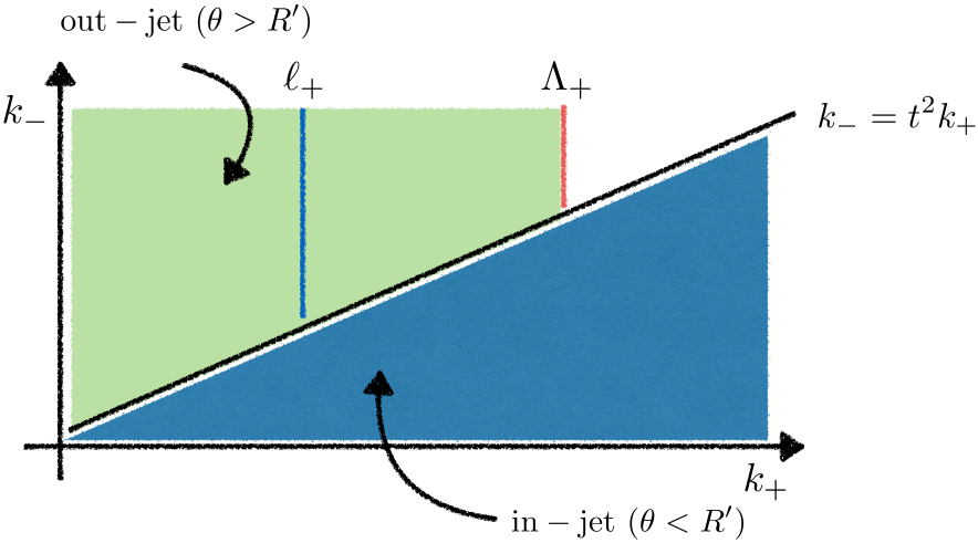
Figure 1: Phase space for the real gluon emission in the collinear-soft function. In the $(k_{+},k_{-})$ plane, the region above the border line $k_{-}=t^{2}k_{+}$ gives the out-jet contribution and the region below gives the in-jet contribution. $\Lambda_{+}$ is the maximum value for the distribution of $\ell_{+}$ and can be chosen arbitrarily.

In Fig. 1 we show the possible phase space for the emitted collinear-soft gluon after the integration over ${\bf{k}}_{\perp}$. $M_{R2}^{S}$ covers region below the jet border line $(k_{-}=t^{2}k_{+})$. Hence the result is

$$M_{R2}^{S} = \frac{\alpha_{s}C_{F}}{\pi}\frac{(\mu^{2}e^{\gamma_{E}})^{\epsilon}}{\Gamma(1-\epsilon)}\delta(\ell_{+})\int^{\infty}_{0}dk_{+}\int^{t^{2}k_{+}}_{0}dk_{-}(k_{+}k_{-})^{-1-\epsilon}$$ (22)

$$= \frac{\alpha_{s}C_{F}}{2\pi}\Biggl{[}\left(\frac{1}{\varepsilon_{\mathrm{UV}}}-\frac{1}{\varepsilon_{\mathrm{IR}}}\right)^{2}-\left(\frac{1}{\varepsilon_{\mathrm{UV}}}-\frac{1}{\varepsilon_{\mathrm{IR}}}\right)\ln t^{2}\Biggr{]}\delta(\ell_{+})_{.}$$

For $M_{R1}^{S}$, $k_{+}$ is fixed to be $\ell_{+}$ by the delta function, and the possible phase space has been denoted as a blue line in the upper plane in Fig 1. However we need to extract the IR divergences as $\ell_{+}\to 0$. In order to do so, we introduce the so called $\Lambda_{+}$-distribution, which is defined as

$$\int_{0}^{L}d\ell_{+}[g(\ell_{+})]_{\Lambda_{+}}f(\ell_{+})=\int_{0}^{L}d\ell_{+}g(\ell_{+})f(\ell_{+})-\int_{0}^{\Lambda_{+}}d\ell_{+}g(\ell_{+})f(0),$$ (23)

where $f(\ell_{+})$ is an arbitrary smooth function at $\ell_{+}=0$. $\Lambda_{+}$ is an arbitrary upper limit for $\Lambda_{+}$-distribution and is power counted to have the same size as $\ell_{+}$. We can write $M_{R1}^{S}$ using this distribution,

$$M_{R1}^{S} = \frac{\alpha_{s}C_{F}}{\pi}\frac{(\mu^{2}e^{\gamma_{E}})^{\epsilon}}{\Gamma(1-\epsilon)}~{}\ell_{+}^{-1-\epsilon}\int^{\infty}_{t^{2}\ell_{+}}dk_{-}k_{-}^{-1-\epsilon}$$ (24)

$$= \delta(\ell_{+})I_{R1}(\Lambda_{+},t)+\frac{\alpha_{s}C_{F}}{\pi}\frac{(\mu^{2}e^{\gamma_{E}})^{\epsilon}}{\Gamma(1-\epsilon)}\Biggl{[}\ell_{+}^{-1-\epsilon}\int^{\infty}_{t^{2}\ell_{+}}k_{-}^{-1-\epsilon}\Biggr{]}_{\Lambda_{+}}\ ,$$

where the integration region for $I_{R1}$ corresponds to the green region in Fig. 1. Integrating over this region, we get

$$I_{R1} = \frac{\alpha_{s}C_{F}}{\pi}\frac{(\mu^{2}e^{\gamma_{E}})^{\epsilon}}{\Gamma(1-\epsilon)}\Biggl{[}\int^{\infty}_{0}dk_{+}\int^{\infty}_{t^{2}k_{+}}dk_{-}(k_{+}k_{-})^{-1-\epsilon}-\int^{\infty}_{\Lambda_{+}}dk_{+}\int^{\infty}_{t^{2}k_{+}}dk_{-}(k_{+}k_{-})^{-1-\epsilon}\Biggr{]}$$

$$= \frac{\alpha_{s}C_{F}}{2\pi}\Biggl{[}\left(\frac{1}{\epsilon_{\mathrm{UV}}}-\frac{1}{\epsilon_{\mathrm{IR}}}\right)^{2}+\left(\frac{1}{\epsilon_{\mathrm{UV}}}-\frac{1}{\epsilon_{\mathrm{IR}}}\right)\ln t^{2}$$

$$~{}~{}~{}~{}~{}~{}-\left(\frac{1}{\epsilon_{\mathrm{UV}}^{2}}+\frac{1}{\epsilon_{\mathrm{UV}}}\ln\frac{\mu^{2}}{\Lambda_{+}^{2}t^{2}}+\frac{1}{2}\ln^{2}\frac{\mu^{2}}{\Lambda_{+}^{2}t^{2}}-\frac{\pi^{2}}{12}\right)\Biggr{]}\ .$$

The second term in Eq. (24) is given by

$$\frac{\alpha_{s}C_{F}}{\pi}\frac{(\mu^{2}e^{\gamma_{E}})^{\epsilon}}{\Gamma(1-\epsilon)}\Biggl{[}\ell_{+}^{-1-\epsilon}\int^{\infty}_{t^{2}\ell_{+}}k_{-}^{-1-\epsilon}\Biggr{]}_{\Lambda_{+}}=\frac{\alpha_{s}C_{F}}{\pi}\Biggl{[}\frac{1}{\ell_{+}}\Bigl{(}\frac{1}{\epsilon_{\mathrm{UV}}}+\ln\frac{\mu^{2}}{\ell_{+}^{2}t^{2}}\Bigr{)}\Biggr{]}_{\Lambda_{+}}\ .$$ (26)

Finally combining Eqs. (20), (22), (II.2) and (26) we obtain the bare one loop result of $\tilde{S}_{q}$,

$$M_{S} = M_{V}^{S}+M_{R1}^{S}+M_{R2}^{S}$$

$$= \frac{\alpha_{s}C_{F}}{\pi}\Biggl{\{}\delta(\ell_{+})\Biggl{(}-\frac{1}{2\epsilon_{\mathrm{UV}}^{2}}-\frac{1}{2\epsilon_{\mathrm{UV}}}\ln\frac{\mu^{2}}{\Lambda_{+}^{2}t^{2}}-\frac{1}{4}\ln^{2}\frac{\mu^{2}}{\Lambda_{+}^{2}t^{2}}+\frac{\pi^{2}}{24}\Biggr{)}$$

$$~{}~{}~{}~{}~{}~{}~{}~{}~{}~{}+\Biggl{[}\frac{1}{\ell_{+}}\Bigl{(}\frac{1}{\epsilon_{\mathrm{UV}}}+\ln\frac{\mu^{2}}{\ell_{+}^{2}t^{2}}\Bigr{)}\Biggr{]}_{\Lambda_{+}}\Biggr{\}}\ .$$

The one loop result of the collinear-soft function for gluon FFJ is the same if we replace $C_{F}$ with $C_{A}=N_{c}$ in Eq. (II.2).

Since the dimensionless soft-collinear function, $S_{k=q,g}(z)=p_{J}^{+}\tilde{S}_{k}(\ell_{+})$, is a function of $z$, we need to express the $\Lambda_{+}$-distribution in terms of the standard plus distribution of $z$. From Eq. (23) we obtain the relation

$$[\tilde{g}(\ell_{+})]_{\Lambda_{+}}=\frac{1}{p_{J}^{+}}[g(z)]_{+}+\frac{1}{p_{J}^{+}}\delta(1-z)\int^{b}_{0}dz^{\prime}g(z^{\prime}),$$ (28)

where $\ell_{+}=p_{J}^{+}(1-z)$ and $g(z)=p_{J}^{+}\tilde{g}(\ell_{+})$. In the $\Lambda_{+}$-distribution, $\Lambda_{+}$ has been replaced with $p_{J}^{+}(1-b)$, where $b$ is a dimensionless parameter close to 1.

Finally, the dimensionless collinear-soft functions at NLO can be written as follows:

$$S_{k=q,g}(z,\mu;(1-z)E_{J}R^{\prime}) = \delta(1-z)+\frac{\alpha_{s}C_{k}}{2\pi}\Biggl{\{}\delta(1-z)\Bigl{(}-\frac{1}{2}\ln^{2}\frac{\mu^{2}}{p_{J}^{+2}t^{2}}+\frac{\pi^{2}}{12}\Bigr{)}$$ (29)

$$~{}~{}~{}~{}~{}~{}~{}~{}~{}~{}~{}~{}+2\Bigl{[}\frac{1}{(1-z)}\Bigl{(}\ln\frac{\mu^{2}}{p_{J}^{+2}t^{2}}-2\ln(1-z)\Bigr{)}\Bigr{]}_{+}\Biggr{\}}\ ,$$

where $C_{q}=C_{F}$ and $C_{g}=C_{A}$. As can be seen in Eq. (29), the scale necessary to minimize the large logarithms in the collinear-soft functions is $(1-z)E_{J}R^{\prime}$. In the limit $z\to 1$, running the collinear-soft function will be required to obtain a precise estimate of the FFJ.

In Eqs. (14) and (17) we have shown the factorization theorem near the endpoint. Combining Eqs. (18), (19) and (29) we can easily check that the fixed NLO results of Eqs. (14) and (17) recover the NLO results of FFJs for the full range Dai:2016hzf ; Kaufmann:2015hma ; Kang:2016mcy when we take the limit $z\to 1$.

III Renormalization Group Evolution and Resummation of Large Logarithms

III.1 RG evolution from the factorization of the FFJ

Based on the factorized results in Eqs. (14) and (17), we can systematically resum the large logarithms of $\ln R$ and $\ln(1-z)$ in the FFJ using the RG evolutions of the integrated jet function $\mathcal{J}_{k}$ and the collinear-soft functions $S_{k}$. The FFJ in the limit $z\to 1$ can be factorized at an arbitrary factorization scale $\mu_{f}$. Then $\mathcal{J}_{k}$ can be evolved from $\mu_{f}$ to collinear scale $\mu_{c}\sim E_{J}R^{\prime}$, where the large logarithms at the higher order in $\alpha_{s}$ are minimized and the perturbative expansion is safely convergent. Simultaneously we can evolve $S_{k}$ from $\mu_{f}$ to $\mu_{cs}\sim(1-z)E_{J}R^{\prime}$ to minimize the large logarithms at $\mu_{cs}$.

The anomalous dimensions of the integrated jet functions and the collinear-soft functions defined by

$$\frac{d}{d\ln\mu}\mathcal{J}_{k}(\mu) = \gamma_{c,k}(\mu)\mathcal{J}_{k}(\mu),$$ (30)

$$\frac{d}{d\ln\mu}S_{k}(x,\mu) = \int^{1}_{x}\frac{dz}{z}\gamma_{cs,k}(z,\mu)S_{k}(x/z,\mu),$$ (31)

where $k=q,~{}g$, are obtained from Eqs. (18), (19), and (29) at one loop,

$$\gamma_{c,q}^{(0)} = \frac{\alpha_{s}C_{F}}{2\pi}\Bigl{(}2\ln\frac{\mu^{2}}{E_{J}^{2}R^{{}^{\prime}2}}+3\Bigr{)}\ ,~{}~{}~{}\gamma_{c,g}^{(0)}=\frac{\alpha_{s}C_{A}}{2\pi}\Bigl{(}2\ln\frac{\mu^{2}}{E_{J}^{2}R^{{}^{\prime}2}}+\frac{\beta_{0}}{C_{A}}\Bigr{)},$$ (32)

$$\gamma_{cs,k}^{(0)}(z) = \frac{\alpha_{s}C_{k}}{2\pi}\Bigl{(}-2\ln\frac{\mu^{2}}{E_{J}^{2}R^{{}^{\prime}2}}\delta(1-z)+\frac{4}{(1-z)_{+}}\Bigr{)}\ ,$$ (33)

where $p_{J}^{+}t$ is approximated as $E_{J}R^{\prime}$. When we combine Eqs. (32) multiplied by $\delta(1-z)$ and Eq. (33), the logarithmic terms cancel and the well-known DGLAP splitting kernels in the limit $z\to 1$ are reproduced:

$$\delta(1-z)\gamma_{c,k}^{(0)}+\gamma_{cs,k}^{(0)}(z)=\frac{\alpha_{s}}{\pi}P_{kk}^{(0)}(z\to 1).$$ (34)

Logarithmic terms in the leading anomalous dimensions indicate the presence of the cusp anomalous dimension. Beyond LL accuracy, the anomalous dimensions can be expressed as

$$\gamma_{c,k} = A_{c}\Gamma_{C,k}(\alpha_{s})\ln\frac{\mu^{2}}{E_{J}^{2}R^{{}^{\prime}2}}+\hat{\gamma}_{c,k}(\alpha_{s}),$$ (35)

$$\gamma_{cs,k}(z) = \delta(1-z)\Bigl{[}A_{cs}\Gamma_{C,k}(\alpha_{s})\ln\frac{\mu^{2}}{E_{J}^{2}R^{{}^{\prime}2}}+\hat{\gamma}_{cs,k}(\alpha_{s})\Bigr{]}-\kappa_{cs}A_{cs}\frac{\Gamma_{C,k}(\alpha_{s})}{(1-z)_{+}}\ ,$$ (36)

where $\Gamma_{C,k}=\sum_{n=0}\Gamma_{n,k}(\alpha_{s}/4\pi)^{n+1}$ are the cusp anomalous dimensions obtained from calculations of light-like Wilson loops Korchemsky:1987wg ; Korchemskaya:1992je . The first two coefficients are given by

$$\Gamma_{0,k}=4C_{k},~{}~{}~{}\Gamma_{1,k}=4C_{k}\Biggl{[}\Bigl{(}\frac{67}{9}-\frac{\pi^{2}}{3}\Bigr{)}C_{A}-\frac{10}{9}n_{f}\Biggr{]}\ .$$ (37)

From the LO results in Eqs. (32) and (33) we extract $\{A_{c},A_{cs},\kappa_{cs}\}=\{1,-1,2\}$ and the noncusp anomalous dimensions $\hat{\gamma}_{c,q}=3\alpha_{s}C_{F}/(2\pi)+\mathcal{O}(\alpha_{s}^{2})$, $\hat{\gamma}_{c,g}=\alpha_{s}\beta_{0}/(2\pi)+\mathcal{O}(\alpha_{s}^{2})$, and $\hat{\gamma}_{cs,k}=\mathcal{O}(\alpha_{s}^{2})$.

Using Eqs. (35) and (36) we perform RG evolutions of the integrated jet functions and the collinear-soft functions up to next-to-leading logarithmic (NLL) accruarcy. For $\mathcal{J}_{k}$ the result of the RG evolution from $\mu_{f}$ to $\mu_{c}$ can be written as

$$\mathcal{J}_{k}(\mu_{f})=\exp\Bigl{[}2A_{c}S_{\Gamma}(\mu_{f},\mu_{c})+A_{c}\ln\frac{\mu_{f}^{2}}{E_{J}^{2}R^{{}^{\prime}2}}a[\Gamma_{C,k}](\mu_{f},\mu_{c})+a[\hat{\gamma}_{c,k}](\mu_{f},\mu_{c})\Bigr{]}\mathcal{J}_{k}(\mu_{c}).$$ (38)

Here $S_{\Gamma}$ and $a[f]$ are

$$S_{\Gamma}(\mu_{f},\mu_{c})=\int^{\alpha_{f}}_{\alpha_{c}}\frac{d\alpha_{s}}{b(\alpha_{s})}\Gamma_{C,k}(\alpha_{s})\int^{\alpha_{s}}_{\alpha_{f}}\frac{d\alpha_{s}^{\prime}}{b(\alpha_{s}^{\prime})},~{}~{}~{}a[f](\mu_{f},\mu_{c})=\int^{\alpha_{f}}_{\alpha_{c}}\frac{d\alpha_{s}}{b(\alpha_{s})}f(\alpha_{s}),$$ (39)

where $\alpha_{f,c}\equiv\alpha_{s}(\mu_{f,c})$ and $b(\alpha_{s})=d\alpha_{s}/(d\ln\mu)$ is QCD beta function.

For the evolution of $S_{k}$, following the conventional method introduced in Refs. Neubert:2005nt ; Becher:2006nr , we obtain

$$S_{k}(z,\mu_{f}) = \exp\Bigl{[}2A_{cs}S_{\Gamma}(\mu_{f},\mu_{cs})+a[\hat{\gamma}_{cs,k}](\mu_{f},\mu_{cs})\Bigr{]}\left(\frac{\mu_{f}^{2}}{E_{J}^{2}R^{{}^{\prime}2}}\right)^{-\eta_{S}/\kappa_{cs}}$$

$$~{}~{}~{}\times\bar{S}_{k}\Bigl{[}\ln\frac{\mu_{cs}^{2}}{E_{J}^{2}R^{{}^{\prime}2}}-2\partial_{\eta_{S}}\Bigr{]}\frac{e^{-\gamma_{E}\eta_{S}}}{\Gamma(\eta_{S})}(1-z)^{(-1+\eta_{S})}\ ,$$

where $\eta_{S}$ is defined as $\eta_{S}=-\kappa_{cs}A_{cs}a[\Gamma_{C,k}](\mu_{f},\mu_{cs})$ and is positive for $\mu_{f}>\mu_{cs}$. $\bar{S}_{k}$ is

$$\bar{S}_{k}[L]=1+\frac{\alpha_{s}C_{k}}{2\pi}\Bigl{(}-\frac{1}{2}L^{2}-\frac{\pi^{2}}{4}\Bigr{)}+\mathcal{O}(\alpha_{s}^{2}).$$ (41)

III.2 Contribution of nonglobal logarithms

When we extend the factorized result of the FFJ to the two loop or higher order in $\alpha_{s}$, one important issue is the presence of nonglobal logarithms (NGLs) Dasgupta:2001sh ; Banfi:2002hw . Usually NGLs appear when jet observables cover a limited phase space due to the jet algorithm and arises from multiple gluon radiations near the jet boundary. Especially when there are large energy differences between in-jet and out-jet radiated gluons, large NGLs are unavoidable.

For the FFJ near the endpoint there are two modes that could resolve the jet boundary and give nonvanishing contributions. The collinear mode with large energy certainly radiates only inside a jet, but the collinear-soft mode can radiate across a jet boundary and give a nonvanishing result as $z\to 1$ at the lower energy scale. So we conjecture there can exist large NGLs in the FFJ in the large $z$ limit.

In order to systematically resum large NGLs, we would need to modify our factorization theorem as it is designed to resum global Sudakov logarithms. To include resummation of NGLs using effective theory, at two loop order we might have to consider dressed collinear-soft gluons decoupled from a (ultra-)collinear gluon along a certain direction inside a jet, which could give rise to a new dipole operator other than $Y_{n,\overline{n}}^{cs}$ at low energy. We will not pursue such a refined factorization theorem here, but we mention that some advanced treatments of NGLs have been recently introduced in Refs. Becher:2015hka ; Becher:2016mmh ; Caron-Huot:2015bja ; Larkoski:2015zka ; Neill:2015nya ; Larkoski:2016zzc ; Becher:2016omr .

To estimate the size of the NGLs in the FFJ, we note that they should have same form as the endpoint logarithms, $\ln(1-z)$, which can be inferred from the ratio of scales between the collinear scale $\mu_{c}\sim E_{J}R^{\prime}$ and the collinear-soft scale $\mu_{cs}\sim(1-z)ER^{\prime}$. As seen in the threshold expansion of inclusive jet production deFlorian:2013qia , leading NGLs start to appear at two loops, $\alpha_{s}^{2}L^{2}\sim\alpha_{s}^{2}(\ln(1-z)/(1-z))_{+}$, where $L$ schematically denotes a large logarithm. So at NLL accuracy we have to resum these leading NGLs to all order in $\alpha_{s}$, i.e., $\sum_{n=2}C_{\rm{NG}}^{n}(\alpha_{s}L)^{n}$.

For the hemisphere jet mass distribution in $e^{+}e^{-}$ annihilation, the resummed result of leading NGLs is known in the large $N_{c}$ limit Dasgupta:2001sh . Interestingly the resummed result of leading NGLs for an individual narrow jet is found to have the same form as the case of the hemisphere jet mass, the only difference simply arising from the need to choose suitable evolution scales Banfi:2010pa ; Dasgupta:2012hg . Therefore, using the result in Ref. Dasgupta:2001sh we conjecture the resummed result of leading NGLs for the FFJ in the large $N_{c}$ limit should be of the form

$$\Delta^{k}_{\mathrm{NG}}(\mu_{c},\mu_{cs})=\exp\Biggl{(}-C_{A}C_{k}\frac{\pi^{2}}{3}\Bigl{(}\frac{1+(at)^{2}}{1+(bt)^{c}}\Bigr{)}t^{2}\Biggr{)}\ ,$$ (42)

where $k=q,~{}g$, and

$$t=\frac{1}{\beta_{0}}\ln{\frac{\alpha_{s}(\mu_{cs})}{\alpha_{s}(\mu_{c})}}\sim-\frac{1}{\beta_{0}}\ln\Bigl{(}1-\frac{\beta_{0}}{4\pi}\alpha_{s}(\mu_{c})\ln\frac{\mu_{c}^{2}}{\mu_{cs}^{2}}\Bigr{)}\ .$$ (43)

The fit parameters from the Monte Carlo implementation of the parton-shower are given by $a=0.85C_{A},~{}b=0.86C_{A}$, and $c=1.33$ Dasgupta:2001sh . Note that our treatment of large logarithm to NLL accuracy only holds for the anti-$\mathrm{k_{T}}$ algorithm. As discussed in Ref. Banfi:2010pa , for other $\mathrm{k_{T}}$-type algorithms, such as $\mathrm{k_{T}}$ and C/A, clustering effects Banfi:2005gj ; Delenda:2006nf give rise to additional large logarithmic terms, which can be also present at NLL order.

Up to NLL accuracy (plus NLO) in $\alpha_{s}$, the resummation factor for NGLs in Eq. (42) just multiplies the resummed results of the FFJ from the previous section, where the resummed expressions of $\mathcal{J}_{k=q,g}$ and $S_{k=q,g}$ are shown in Eqs. (38) and (III.1) respectively. In the next section we show various numerical results for the FFJ in the large $z$ region comparing the results using only DGLAP evolutions and our resummed results of the large logarithms as well as the NGLs.

IV Numerical Results

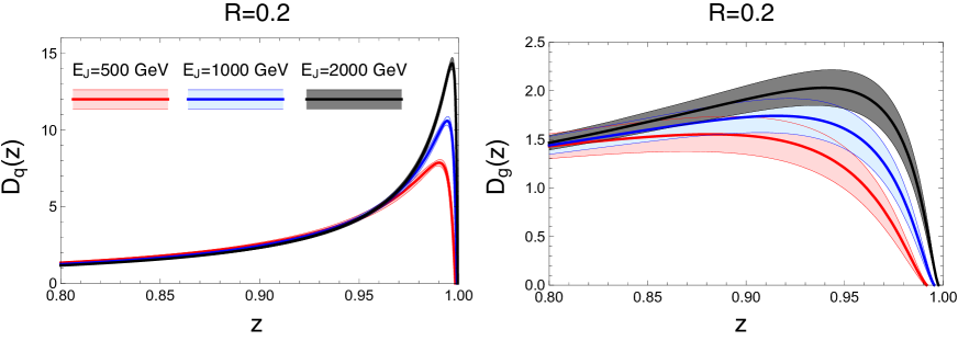
Figure 2: $D_{J_{q}/q}(z)$ (left panel) and $D_{J_{g}/g}(z)$ (right panel) with different jet energies. Red, blue, and black curves correspond to jet energy $E_{J}$ equal to 500, 1000, and 2000 GeV, respectively. The jet radius is chosen to be $R=0.2$ and the factorization scale is $\mu_{f}=E_{J}$. Error estimation is described in the text.

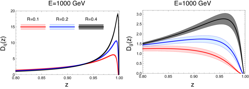
Figure 3: $D_{J_{q}/q}(z)$ (left panel) and $D_{J_{g}/g}(z)$ (right panel) with different jet radii. Red, blue, and black curves correspond to the jet radius $R$ equal to $0.1$, $0.2$, and $0.4$ respectively. The jet energy is $E_{J}=1000$ GeV and the factorization scale is $\mu_{f}=E_{J}$.

In this section we show numerical results of the resummed FFJ focusing on the large $z$ region. For simplicity we set $R^{\prime}=R$. As shown in sec. III.1, in order to resum large logarithms in $D_{J_{k}/k}(z,\mu_{f})$, the integrated jet functions ${\cal J}_{k}$ are run from the jet scale $\mu_{c}=ER$ to $\mu_{f}$, and the collinear-soft functions $S_{k}$ from $\mu_{cs}=ER(1-z)$ to $\mu_{f}$. Because the FFJ is dependent upon the scale $\mu_{f}$ (actually following DGLAP evolution), the shape of the FFJ varies for different choices of $\mu_{f}$. For convenience we choose $\mu_{f}=E_{J}$ throughout this section. Error estimations of the jet and the collinear-soft functions are obtained by varying the jet scale and the collinear-soft scale within $(\mu_{c}/2,2\mu_{c})$ and $(\mu_{cs}/2,2\mu_{cs})$ respectively. Then errors of $D_{J_{k}/k}(z,\mu_{f})$ are obtained by summing these in quadrature.

Based on the factorized expressions in Eqs. (14) and (17), Fig. 2 shows $\mathrm{NLL_{G}+NLO}$ results of $D_{J_{q}/q}$ and $D_{J_{g}/g}$ for different energies of jets with the same radius $R=0.2$. Here $\mathrm{NLL_{G}}$ represents the NLL accuracy including only global logarithms from the factorization approach in sec. III.1. For the extreme endpoint region where $\mu_{cs}=E_{J}R(1-z)\approx\Lambda_{\rm QCD}$, our description is not reliable because of nonperturbative contributions. Fig. 3 shows $\mathrm{NLL_{G}+NLO}$ results of $D_{J_{q}/q}$ and $D_{J_{g}/g}$ for different jet radii with the jet energy fixed to be 1000 GeV. From Figs. 2 and 3 we can see the tendencies that energetic parton showering processes are captured more in the jet as the jet energy $E_{J}$ and/or the radius $R$ become larger.

To see the importance of the factorization description on the FFJs, in Fig. 4 we compare the resummed results at $\mathrm{NLL_{G}+NLO}$ and the results using leading DGLAP evolution naively. Here using only DGLAP evolution from $\mu_{c}=E_{J}R$ to $\mu_{f}=E_{J}$ can be understood as resumming only large logarithms of $R$. As $z$ goes to 1, the resummed results of only $\ln R$ blow up. However, when we do DGLAP evolution from $\mu_{cs}=E_{J}R(1-z)$ to $\mu_{f}=E_{J}$, we can see more realistic results. Compared with our factorization approach with the accuracy of $\mathrm{NLL_{G}+NLO}$, both DGLAP evolved results involve much larger uncertainties.

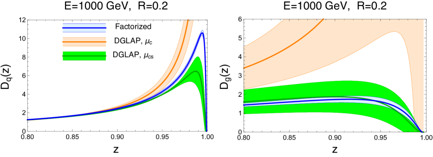
Figure 4: Comparison of the result using leading DGLAP evolution and the resummed result at $\mathrm{NLL_{G}+NLO}$ from the factorization approach. The orange (green) curves are obtained using leading DGLAP evolution with FFJs running from $\mu_{c}=E_{J}R~{}(\mu_{cs}=E_{J}R(1-z))$ to $\mu_{f}=E_{J}$. Blue curves are the resummed result of the FFJs. The jet radius is $R=0.2$ and jet energy is $E_{J}=1000$ GeV.

Fig. 5 shows the resummed result of the FFJs with the accuracy of $\mathrm{NLL_{G+NG}+NLO}$ using our conjectured result for including leading NGLs discussed in sec. III.2, obtained by multiplication of the FFJ at $\mathrm{NLL_{G}+NLO}$ by $\Delta^{k=q,g}_{\mathrm{NG}}(\mu_{c},\mu_{cs})$ in Eq. (42). The result including leading NGLs gives rise to some suppression to the FFJs. A similar suppression can be also seen in the light jet mass distribution for the hemisphere jet production when the resummed results including the NGLs are compared with the case without the NGLs Becher:2016omr . Because of additional dependences on both $\mu_{c}$ and $\mu_{cs}$ from $\Delta^{k=q,g}_{\mathrm{NG}}(\mu_{c},\mu_{cs})$, the result with NGLs increases the errors. The errors might be reduced if we include the NNLO result in $\alpha_{s}$, which is beyond the scope of our paper.

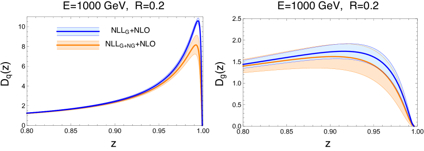
Figure 5: Comparison of the resummed results with (orange) and without (blue) resumming the NGLs. Here $R=0.2$ and $E_{J}=1000$ GeV.

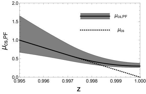
Figure 6: Profile function $\mu_{cs,PF}$ [solid black curve and gray band, defined in Eq. (44)] is used to estimate errors due to variation of the collinear-soft scale. The dashed line is the $z$ dependent collinear-soft scale $\mu_{c}(1-z)$ with $\mu_{c}=200$ GeV.

There is one more comment about error estimations used above. Since $\mu_{cs}=E_{J}R(1-z)$ is $z$ dependent and bound to hit the Landau pole as $z\to 1$, we have used the following profile function to avoid the Landau pole:

$$\mu_{cs,PF}(z)=(1+\frac{\delta}{1+{\rm exp}[(z-z_{1})/(1-z_{1})]})\begin{cases}(1-z)\mu_{c}&\text{if }z<z_{1}\\ \mu_{\rm Min}+a(1-z)^{2}&\text{if }z\geq z_{1}\end{cases},$$ (44)

where $\mu_{\rm Min}=0.3$, $\mu_{c}=E_{J}R$, $a$ and $z_{1}$ are fixed by requiring that $\mu_{cs,PF}(z)$ and its first derivative are continuous at $z=z_{1}$. The profile function is shown in Fig. 6. To vary the collinear-soft scale, we used $\delta=\{0,-0.5,1\}$. $\mu_{cs,PF}(z)$ is devised to ensure that the collinear-soft scale freezes as it approaches the Landau pole and coincide with $\mu_{cs}(z)$ otherwise.

V Conclusion and Outlook

In this paper, as shown in Eqs. (14) and (17), we have developed a factorization theorem of the FFJ with a small jet radius $R$ in the large $z$ limit. At the scale $\mu\sim E_{J}R^{\prime}$ we first integrate out collinear modes with offshellness $p_{c}^{2}\sim(E_{J}R^{\prime})^{2}$, and obtain the integrated jet functions, $\mathcal{J}_{q,g}$. At the lower scale $\mu\sim(1-z)E_{J}R^{\prime}$ the collinear-soft mode can probe the jet boundary and gives a nonvanishing result at higher order in $\alpha_{s}$. Combining NLO results of the integrated jet function and the collinear-soft function, we can successfully reproduce NLO result of the FFJ in the limit $z\to 1$.

Performing RG evolutions of the factorized jet and collinear-soft functions we resummed large logarithms of $1-z$ and $R$ simultaneously. The anomalous dimensions of each factorized function involves the cusp anomalous dimension, which enables us to systematically resum large logarithms beyond leading order. As a result we have shown the resummed result at NLL, which significantly modifies the large $z$ behavior of the FFJ when compared to the result of only resuming logarithms of $R$ through naive DGLAP evolution. Large NGLs may appear at NNLO in $\alpha_{s}$ and could contribute to the resummed result at NLL accuracy. We therefore have estimated NGL contributions to the FFJ applying the resummed formalism in the large $N_{c}$ limit Dasgupta:2001sh .

The finite size of the jet radius $R$ plays an important role in performing successful RG evolution of the FFJ in the large $z$ limit. Even though $R$ is small, the radius makes it possible to have an observed jet with nonzero invariant mass and each factorized function for the FFJ is IR finite. Similar results occur for the heavy quark fragmentation function (HQFF) in the large $z$ limit, where the HQFF can be factorized into the heavy quark function and the soft shape function Neubert:2007je ; Fickinger:2016rfd . Due to a nonzero heavy quark mass $M$, both functions are IR finite and systematic RG evolutions to the scales $M$ and $M(1-z)$ can be done.

Note that the FFJ reduces to a light hadron fragmentation function if $R$ goes to zero. In this case the factorization to collinear and collinear-soft interactions breaks down because the relevant anomalous dimensions blow up and RG evolutions become nonperturbative, as can be checked from Eqs. (32) and (33). A similar result can be applied to the parton distribution function (PDF) near the endpoint. Actually, in order to resum large logarithm $\ln(1-z)$ in the PDF, a similar factorization approach to ours has been considered in Ref. Fleming:2012kb , where soft gluon radiation is responsible for the parton splitting. Interestingly the factorized collinear and soft functions for the PDF contains rapidity divergences Chiu:2011qc ; Chiu:2012ir as well as UV and IR divergences. However the rapidity RG evolution turns out to be IR sensitive and become nonperturbative. (We checked if there exist rapidity divergences in the factorized functions for the FFJ, but the finite size of $R$ forbids rapidity divergences and guarantees ordinary RG evolutions from pure UV divergences.)

Our factorized and resummed result analyzed here can be widely applied for energetic jet productions. The resumming procedure of large logarithms of $1-z$ from the effective theory approach can be used for systematic resummations of threshold logarithms for inclusive jet deFlorian:2013qia ; deFlorian:2007fv and dijet production Kidonakis:1998bk ; Hinderer:2014qta . However, for more precisely resummed results of large logarithms, explicit calculations beyond NLO are required, and a thorough analysis of factorization including NGLs is needed.

- (1) J. C. Collins and D. E. Soper, Nucl. Phys. B 194, 445 (1982).
- (2) A. Metz and A. Vossen, Prog. Part. Nucl. Phys. 91, 136 (2016) [arXiv:1607.02521 [hep-ex]].
- (3) S. Catani, Y. L. Dokshitzer, M. H. Seymour and B. R. Webber, Nucl. Phys. B 406, 187 (1993).
- (4) S. D. Ellis and D. E. Soper, Phys. Rev. D 48, 3160 (1993) [hep-ph/9305266].
- (5) Y. L. Dokshitzer, G. D. Leder, S. Moretti and B. R. Webber, JHEP 9708, 001 (1997) [hep-ph/9707323].
- (6) G. P. Salam and G. Soyez, JHEP 0705, 086 (2007) [arXiv:0704.0292 [hep-ph]].
- (7) M. Cacciari, G. P. Salam and G. Soyez, JHEP 0804, 063 (2008) [arXiv:0802.1189 [hep-ph]].
- (8) M. Dasgupta, F. Dreyer, G. P. Salam and G. Soyez, JHEP 1504, 039 (2015) [arXiv:1411.5182 [hep-ph]].
- (9) S. Sapeta, Prog. Part. Nucl. Phys. 89, 1 (2016) [arXiv:1511.09336 [hep-ph]].
- (10) M. Procura and W. J. Waalewijn, Phys. Rev. D 85, 114041 (2012) [arXiv:1111.6605 [hep-ph]].
- (11) M. Baumgart, A. K. Leibovich, T. Mehen and I. Z. Rothstein, JHEP 1411, 003 (2014) [arXiv:1406.2295 [hep-ph]].
- (12) T. Kaufmann, A. Mukherjee and W. Vogelsang, Phys. Rev. D 92, no. 5, 054015 (2015) [arXiv:1506.01415 [hep-ph]].
- (13) Y. T. Chien, Z. B. Kang, F. Ringer, I. Vitev and H. Xing, JHEP 1605, 125 (2016) [arXiv:1512.06851 [hep-ph]].
- (14) L. Dai, C. Kim and A. K. Leibovich, Phys. Rev. D 94, no. 11, 114023 (2016) [arXiv:1606.07411 [hep-ph]].
- (15) Z. B. Kang, F. Ringer and I. Vitev, JHEP 1611, 155 (2016) [arXiv:1606.07063 [hep-ph]].
- (16) A. Idilbi and C. Kim, arXiv:1606.05429 [hep-ph].
- (17) R. Bain, Y. Makris and T. Mehen, JHEP 1611, 144 (2016) [arXiv:1610.06508 [hep-ph]].
- (18) D. Neill, I. Scimemi and W. J. Waalewijn, arXiv:1612.04817 [hep-ph].
- (19) M. Procura and I. W. Stewart, Phys. Rev. D 81, 074009 (2010) Erratum: [Phys. Rev. D 83, 039902 (2011)] [arXiv:0911.4980 [hep-ph]].
- (20) A. Jain, M. Procura and W. J. Waalewijn, JHEP 1105, 035 (2011) [arXiv:1101.4953 [hep-ph]].
- (21) M. Ritzmann and W. J. Waalewijn, Phys. Rev. D 90, no. 5, 054029 (2014) [arXiv:1407.3272 [hep-ph]].
- (22) Z. B. Kang, F. Ringer and I. Vitev, JHEP 1610, 125 (2016) [arXiv:1606.06732 [hep-ph]].
- (23) M. Dasgupta, F. A. Dreyer, G. P. Salam and G. Soyez, JHEP 1606, 057 (2016) [arXiv:1602.01110 [hep-ph]].
- (24) C. W. Bauer, S. Fleming and M. E. Luke, Phys. Rev. D 63, 014006 (2000) [hep-ph/0005275].
- (25) C. W. Bauer, S. Fleming, D. Pirjol and I. W. Stewart, Phys. Rev. D 63, 114020 (2001) [hep-ph/0011336].
- (26) C. W. Bauer, D. Pirjol and I. W. Stewart, Phys. Rev. D 65, 054022 (2002) [hep-ph/0109045].
- (27) C. W. Bauer, S. Fleming, D. Pirjol, I. Z. Rothstein and I. W. Stewart, Phys. Rev. D 66, 014017 (2002) [hep-ph/0202088].
- (28) C. W. Bauer, F. J. Tackmann, J. R. Walsh and S. Zuberi, Phys. Rev. D 85, 074006 (2012) [arXiv:1106.6047 [hep-ph]].
- (29) M. Procura, W. J. Waalewijn and L. Zeune, JHEP 1502, 117 (2015) [arXiv:1410.6483 [hep-ph]].
- (30) T. Becher, M. Neubert, L. Rothen and D. Y. Shao, Phys. Rev. Lett. 116, no. 19, 192001 (2016) [arXiv:1508.06645 [hep-ph]].
- (31) Y. T. Chien, A. Hornig and C. Lee, Phys. Rev. D 93, no. 1, 014033 (2016) [arXiv:1509.04287 [hep-ph]].
- (32) T. Becher, M. Neubert, L. Rothen and D. Y. Shao, JHEP 1611, 019 (2016) [arXiv:1605.02737 [hep-ph]].
- (33) D. W. Kolodrubetz, P. Pietrulewicz, I. W. Stewart, F. J. Tackmann and W. J. Waalewijn, JHEP 1612, 054 (2016) [arXiv:1605.08038 [hep-ph]].
- (34) M. Dasgupta and G. P. Salam, Phys. Lett. B 512, 323 (2001) [hep-ph/0104277].
- (35) A. Banfi, G. Marchesini and G. Smye, JHEP 0208, 006 (2002) [hep-ph/0206076].
- (36) S. D. Ellis, C. K. Vermilion, J. R. Walsh, A. Hornig and C. Lee, JHEP 1011, 101 (2010) [arXiv:1001.0014 [hep-ph]].
- (37) A. V. Manohar and I. W. Stewart, Phys. Rev. D 76, 074002 (2007) [hep-ph/0605001].
- (38) C. W. Bauer, D. Pirjol and I. W. Stewart, Phys. Rev. D 68, 034021 (2003) [hep-ph/0303156].
- (39) J. Chay, C. Kim, Y. G. Kim and J. P. Lee, Phys. Rev. D 71, 056001 (2005) [hep-ph/0412110].
- (40) W. M. Y. Cheung, M. Luke and S. Zuberi, Phys. Rev. D 80, 114021 (2009) [arXiv:0910.2479 [hep-ph]].
- (41) J. Chay, C. Kim and I. Kim, Phys. Rev. D 92, no. 3, 034012 (2015) [arXiv:1505.00121 [hep-ph]].
- (42) G. P. Korchemsky and A. V. Radyushkin, Nucl. Phys. B 283, 342 (1987).
- (43) I. A. Korchemskaya and G. P. Korchemsky, Phys. Lett. B 287, 169 (1992).
- (44) M. Neubert, Phys. Rev. D 72, 074025 (2005) [hep-ph/0506245].
- (45) T. Becher and M. Neubert, Phys. Rev. Lett. 97, 082001 (2006) [hep-ph/0605050].
- (46) S. Caron-Huot, arXiv:1501.03754 [hep-ph].
- (47) A. J. Larkoski, I. Moult and D. Neill, JHEP 1509, 143 (2015) [arXiv:1501.04596 [hep-ph]].
- (48) D. Neill, arXiv:1508.07568 [hep-ph].
- (49) A. J. Larkoski, I. Moult and D. Neill, JHEP 1611, 089 (2016) [arXiv:1609.04011 [hep-ph]].
- (50) T. Becher, B. D. Pecjak and D. Y. Shao, JHEP 1612, 018 (2016) [arXiv:1610.01608 [hep-ph]].
- (51) D. de Florian, P. Hinderer, A. Mukherjee, F. Ringer and W. Vogelsang, Phys. Rev. Lett. 112, 082001 (2014) [arXiv:1310.7192 [hep-ph]].
- (52) A. Banfi, M. Dasgupta, K. Khelifa-Kerfa and S. Marzani, JHEP 1008, 064 (2010) [arXiv:1004.3483 [hep-ph]].
- (53) M. Dasgupta, K. Khelifa-Kerfa, S. Marzani and M. Spannowsky, JHEP 1210, 126 (2012) [arXiv:1207.1640 [hep-ph]].
- (54) A. Banfi and M. Dasgupta, Phys. Lett. B 628, 49 (2005) [hep-ph/0508159].
- (55) Y. Delenda, R. Appleby, M. Dasgupta and A. Banfi, JHEP 0612, 044 (2006) [hep-ph/0610242].
- (56) N. Kidonakis, G. Oderda and G. F. Sterman, Nucl. Phys. B 525, 299 (1998) [hep-ph/9801268].
- (57) M. Neubert, arXiv:0706.2136 [hep-ph].
- (58) M. Fickinger, S. Fleming, C. Kim and E. Mereghetti, JHEP 1611, 095 (2016) [arXiv:1606.07737 [hep-ph]].
- (59) S. Fleming and O. Z. Labun, Phys. Rev. D 91, no. 9, 094011 (2015) [arXiv:1210.1508 [hep-ph]].
- (60) J. y. Chiu, A. Jain, D. Neill and I. Z. Rothstein, Phys. Rev. Lett. 108, 151601 (2012) [arXiv:1104.0881 [hep-ph]].
- (61) J. Y. Chiu, A. Jain, D. Neill and I. Z. Rothstein, JHEP 1205, 084 (2012) [arXiv:1202.0814 [hep-ph]].
- (62) D. de Florian and W. Vogelsang, Phys. Rev. D 76, 074031 (2007) [arXiv:0704.1677 [hep-ph]].
- (63) P. Hinderer, F. Ringer, G. F. Sterman and W. Vogelsang, Phys. Rev. D 91, no. 1, 014016 (2015) [arXiv:1411.3149 [hep-ph]].