Trapped modes in zigzag graphene nanoribbons

Abstract

We study a scattering on an ultra-low potential in zigzag graphene nanoribbon. Using mathematical framework based on the continuous Dirac model and augumented scattering matrix, we derive a condition for the existence of a trapped mode. We consider the threshold energies where the continuous spectrum changes its multiplicity and show that the trapped modes may appear for energies slightly less than a threshold and its multiplicity does not exceeds one. We prove that trapped modes do not appear outside the threshold, provided the potential is sufficiently small.

1 Introduction

The problem of disorder in graphene nanoribbons has been studied extensively. The main purpose of those studies is to eliminate disorder completely and produce pure high-quality graphene nanoribbons [7]. Approaching the goal of graphene nanoribbons free of impurities and other defects one can focus on production of such deliberately for the use in electronic devices. One of desired features for graphene to possess is a possibility of electron localization. Such localization is difficult to achieve due to Klein tunneling [10]. As graphene electrons behave like massless particles they undergo tunneling through barriers. However, due to interference between continuous states of the nanoribbon and a localized state of a disorder, a trapped mode can be produced. There are several types of disorder including short-range and long-range. Impurities such as vacancies and adatoms are classified as short-range type and can be described by a sharp potential, that varies on the scale shorter than graphene lattice constant (0.246 nm) [2]. On the other hand, electric or magnetic field, interactions with substrate, Coulomb charges [13], ripples and wrinkles can lead to long-range disorder described by smooth potential (a Gaussian for example). In the present studies we assume that graphene is free of short-range defects and the potential is modeled as a long range one.

There are two groups of graphene nanoribbons, that differ by the edge type and are called zigzag and armchair [4, 5]. In this paper, we give a condition for existence and a choice of ultra-low potential that produces a trapped mode in zigzag graphene nanoribbon. We work within continuous Dirac model, where graphene is isotropic and its electrons dynamics can be described by a system of 4 equations [5]

$$\left(\begin{array}[]{cccc}0&i\partial_{x}+\partial_{y}&0&0\\ i\partial_{x}-\partial_{y}&0&0&0\\ 0&0&0&-i\partial_{x}+\partial_{y}\\ 0&0&-i\partial_{x}-\partial_{y}&0\end{array}\right)+\delta\mathcal{P}\left(\begin{array}[]{c}u^{\prime}\\ v^{\prime}\\ u\\ v\end{array}\right)=\omega\left(\begin{array}[]{c}u^{\prime}\\ v^{\prime}\\ u\\ v\end{array}\right),$$ (1)

where $\omega=\frac{E}{\hbar\nu_{F}}$ is scaled energy (with $E$ denoting energy and $\nu_{F}\approx 10^{6}\frac{m}{s}$ Fermi velocity), a potential $\mathcal{P}$ is a real-value function with compact support such that $\sup|\mathcal{P}|\leq 1$ and $\delta$ is a real-value small parameter.

The number of equation is a consequence of the discrete description of graphene lattice and low energy approximation which leads to the continuous model [5, 15]. In the discrete model graphene is described as a composition of two triangular interpenetrating lattices of carbon atoms (called A and B) [5]. Then low energy approximation can be done in a twofold way, close to two different energy minima (called $K$ and $K^{\prime}$) in the graphene dispersion relation. Consequently, in the continuous model, we have two waves that describe an electron in any single point of the ribbon (A or B) coupled in two different ways, close to $K$ (first two equations in (1)) or $K^{\prime}$ point (last two equations in (1)). A nanoribbon is modeled as an unit strip $\Pi=(0,1)\times\mathbb{R}$ due to rescaling. The zigzag boundary of the nanoribbon requires one wave (A) to disappear specifically at one edge and the other (B) at the other one [4]

$$u^{\prime}(0,y)=0\ ,\ \ u(0,y)=0\ ,\ \ v^{\prime}(1,y)=0\ ,\ \ v(1,y)=0\;.$$ (2)

As our potential $\mathcal{P}$ is assumed to be of long-range type, it can be described by a diagonal matrix with equal elements [2]. As neither the potential nor the boundary conditions couples $K$ and $K^{\prime}$ valleys, the system of 4 equations can be split into two systems of 2 equations where only intravalley scattering is allowed. We consider one of them (two last equations in (1))

$$\left(\begin{array}[]{cc}0&-i\partial_{x}+\partial_{y}\\ -i\partial_{x}-\partial_{y}&0\end{array}\right)\left(\begin{array}[]{c}u\\ v\end{array}\right)+\delta\mathcal{P}\left(\begin{array}[]{c}u\\ v\end{array}\right)=\omega\left(\begin{array}[]{c}u\\ v\end{array}\right)$$ (3)

supplied with the boundary conditions:

$$u(0,y)=0\ ,\ \ v(1,y)=0.$$ (4)

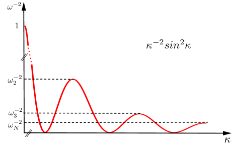
Figure 1: Dispersion with energy thresholds.

Energy threshold $\omega=\omega_{N}>1$, $N=2,\,3,\dots$ is defined by one of maxima in zigzag dispersion relation $\omega^{-2}=\kappa^{-2}\sin^{2}\kappa$ and it reads $\frac{d}{d\kappa}\Big{(}\kappa^{-2}\sin^{2}\kappa\Big{)}=0$ (see Figure 1). The index $N$ defines a threshold energy $\omega_{N}$ as it indicates change of the multiplicity of the continuous spectrum from $2N-3$ to $2N-1$ for $N\geq 2$. A trapped mode is defined as a vector eigenfunction (from $L_{2}$ space) that corresponds to an eigenvalue embedded in the continuous spectrum. The main result of the paper is the following theorem about existence of trapped modes in zigzag graphene nanoribbon for energies close to one of the thresholds that can be chosen arbitrary.

Theorem 1.1.

For every $N=2,\,,3,\,...$ there exists $\varepsilon_{N}>0$ such that for each $\varepsilon\in(0,\varepsilon_{N})$ there exists $\delta\sim\sqrt{\varepsilon}$ and a potential $\mathcal{P}$ such that the problem (3), (4) has a trapped mode solution for $\omega^{-1}=\omega_{N}^{-1}+\varepsilon$.

Second result shows that trapped modes may appear only for energy slightly smaller than threshold and that spectrum far from the threshold is free of embedded eigenvalues. Moreover their multiplicity does not exceed one.

Theorem 1.2.

There exist positive numbers $\varepsilon_{0}$ and $\delta_{0}$, which may depend on $N$, such that if

(i) $\omega\in[\omega_{N},\,\omega_{N}+\varepsilon_{0}]$ and $|\delta|<\delta_{0}$, then problem (3), (4) has no trapped modes;

(ii) $\omega\in[\omega_{N}-\varepsilon_{0},\,\omega_{N})$ and $|\delta|<\delta_{0}$, then the multiplicity of a trapped mode to problem (3), (4) does not exceed $1$.

(iii) For every $\varepsilon_{1}>0$ and $C_{1}>0$ there exist $\delta_{1}>0$ such that if $0\leq\omega<C_{1}$ and $|\omega-\omega_{N}|>\varepsilon_{1}$ for all $N=2,\ldots$ satisfying $\omega_{N}\leq C_{1}$ and $|\delta|<\delta_{1}$, then problem (3), (4) has no trapped modes.

Those results come from the analysis of the trapped modes in the $K^{\prime}$ valley (system (3), (4)), however the analysis in the $K$ valley (first two equations in (1) with boundary conditions (2)) is analogous and requires complex conjugation only.

The continuous spectrum of the problem (3), (4) with $\mathcal{P}=0$ covers the whole real axis and, hence, its eigenvalues, if exist, possess the natural instability, that is, a small perturbation may lead them out from the spectrum and turn into points of complex resonance, cf. [3, 21] and the review paper [14]. A few of approaches have been proposed to compensate for this instability and to detect eigenvalues embedded into the continuous spectrum. First of all, a simple but very elegant trick was developed in [8] for scalar problems. Namely, under a symmetry assumption on waveguide’s shape an artificial Dirichlet condition is imposed on the mid-hyperplane of the waveguide which shifts the lower bound of the spectrum above and allows to apply the variational or asymptotic method to find out a point in the discrete spectrum of the reduced problem. At the same time, the odd extension of the corresponding eigenfunciton through the Dirichlet hyperplane gives an eigenfunction of the original problem so that it remains to verify that the eigenvalue falls into the original continuous spectrum. In other words, the problem operator is restricted into a subspace where it may get the discrete spectrum which becomes a part of the point spectrum in the complete setting. For vectorial problems the existence of such invariant subspaces usually demand very strong conditions on physical and geometrical properties of waveguides and therefore the trick works rather rarely or needs supplementary ideas, cf. [24, 9] and [18]. Unfortunately, the Dirac equations do not possess the necessary properties and we are not able to find a way to apply the trick in our problem.

Another approach accepting formally self-adjoint elliptic systems but employing much more elaborated asymptotic analysis is based on the concept of enforced stability of embedded eigenvalues [20, 21, 22]. In this way, having an eigenvalue in the continuous spectrum of a waveguide with $N$ open channels for wave propagation one can select a small perturbation of the problem by means of tuning $N$ parameters such that, although the eigenvalue enjoys a perturbation, it remains sitting on the real axis and does not move into the complex plane. It is remarkable that, as it was shown in a different situations [20, 19, 21, 6] and others, it is possible to take as an "initiator" of a trapped mode a particular standing wave at the threshold value of the spectral parameter and by an appropriate choice of the perturbation parameters to construct an eigenvalue which is situated near but only on one side of the threshold so that it belongs to the continuous spectrum. This method was introduced and developed in [20, 21, 22]. Aiming to apply it for detection of eigenvalues for the zigzag graphene nanoribbon, we unpredictably observed that the corresponding boundary value problem in whole is not elliptic (see Appendix A). As a result, many steps of the detection procedure require serious modifications.

The paper is organized as follows. In Sect. 2 we analyse Dirac model without potential. For each non-zero energy we construct all bounded solutions and identify thresholds where the dimension of the space of such solution changes. We construct also unbounded solutions near threshold and introduce a symplectic form, which will play an important role in the study of the scattering problem. These unbounded solutions are studied in Sect. 2.4, 2.8 and 2.9. In Sect. 2.10, we present a solvability result for non-homogenous problem. In Sect. 3 we add potential to the model, and consider scattering problem with the use of artificial augumented scattering matrix introduced in Sect. 3.2. In Sect. 4 we analyze trapped modes, providing in Sect. 4.1 a necessary and sufficient condition for their existence, from which in Sect. 4.2 we extract the potential description and prove Theorem 1.1. Finally, in the last section, Sect. 4.3, we analyze the multiplicity of trapped modes proving Theorem 1.2.

2 Dirac equation

2.1 Problem statement

We consider problem (3) without potential ($\mathcal{P}=0$)

$${\mathcal{D}}\left(\begin{array}[]{c}u\\ v\end{array}\right)=\omega\left(\begin{array}[]{c}u\\ v\end{array}\right),\;\;\;{\mathcal{D}}={\mathcal{D}}(\partial_{x},\partial_{y}):=\left(\begin{array}[]{cc}0&-i\partial_{x}+\partial_{y}\\ -i\partial_{x}-\partial_{y}&0\end{array}\right)$$ (5)

supplied with the boundary conditions (4). Our goal is to find solutions to this problem, especially bounded ones and thereby describe continuous spectrum of the operator corresponding to (5), (4).

Let us introduce the spaces

$$X=\{u\in L^{2}(\Pi)\,:\,(i\partial_{x}+\partial_{y})u\in L^{2}(\Pi),\;\mbox{and}\;\;u(0,y)=0\}$$

and

$$Y=\{v\in L^{2}(\Pi)\,:\,(-i\partial_{x}+\partial_{y})v\in L^{2}(\Pi),\;\mbox{and}\;\;v(1,y)=0\}.$$

Then ${\mathcal{D}}$ is a self-adjoint operator in $L^{2}(\Pi)\times L^{2}(\Pi)$ with the domain $X\times Y$.

We note that for $\omega=0$ we have $(-i\partial_{x}+\partial_{y})v=(-i\partial_{x}-\partial_{y})u=0$ therefore $u=u(-x+iy)$ and $v=v(x+iy)$ what together with $u(0,y)=0\ ,v(1,y)=0$ give $u=0\ ,v=0$. There are no non-trivial solutions to (5), (4) for $\omega=0$.

Now, assume that $\omega\neq 0$, then problem (5), (4) can be written as the system

$$-\Delta u=\omega^{2}u\ ,\ \ v=\frac{1}{\omega}(-i\partial_{x}-\partial_{y})u\ ,\ \ u(0,y)=0\ ,\ \ v(1,y)=0.$$ (6)

We are looking for non-trivial solutions which are exponential (or possibly power exponential) in $y$, i.e.

$$(u(x,y),v(x,y))=e^{-i\lambda y}(\mathcal{U}(x),\mathcal{V}(x)),$$ (7)

$\lambda$ is a component of a wave vector parallel with the nanoribbons edge. Then insertion into (6) gives

$$\begin{cases}-\mathcal{U}_{xx}=(\omega^{2}-\lambda^{2})\mathcal{U}\ ,\ \ \mathcal{U}(0)=0,\ \ \ \ \mathcal{U}_{x}(1)=\lambda\mathcal{U}(1),\\ \mathcal{V}=\frac{1}{\omega}(-i\mathcal{U}_{x}+i\lambda\mathcal{U}).\end{cases}$$ (8)

Lemma 1.

If (7) is a non-trivial solution to (5), (4) with a certain complex $\lambda$ then: (i) $\Im\lambda=0$ or (ii) $\Im\lambda\neq 0$ and $\Re\lambda>0$.

Proof.

Multiplying the first equation in (8) by $\overline{\mathcal{U}}$ and integrating in $x\in(0,1)$, we have

$$\int_{0}^{1}(\omega^{2}-\lambda^{2})\mathcal{U}\overline{\mathcal{U}}dx=-\int_{0}^{1}\mathcal{U}_{xx}\overline{\mathcal{U}}dx=\int_{0}^{1}\mathcal{U}_{x}\overline{\mathcal{U}}_{x}dx-\lambda\mathcal{U}(1)\overline{\mathcal{U}}(1)$$

Taking the imaginary part of this equation, we get

$$2\Re\lambda\,\Im\lambda\int_{0}^{1}\mathcal{U}\,\overline{\mathcal{U}}dx=\Im\lambda\mathcal{U}(1)\,\overline{\mathcal{U}}(1).$$

Therefore, if $\Im\lambda\neq 0$, then $\Re\lambda$ must be positive provided $\mathcal{U}\neq 0$. ∎

Consider the case $\lambda^{2}=\omega^{2}$. Then there exists an exponential solution only for $\lambda=1$ and it has the following form

$$\mathcal{U}(x)=x\ ,\ \ \mathcal{V}(x)=i\frac{1}{\omega}(x-1).$$ (9)

Let $\lambda^{2}\neq\omega^{2}$. Then the solution to (8) is given by

$$\mathcal{U}(x)=\sin(\kappa x)\ ,\ \ \mathcal{V}(x)=\pm i\sin(\kappa(x-1)),$$ (10)

where $\kappa$ satisfies

$$\frac{\sin\kappa}{\kappa}=\pm\frac{1}{\omega}$$ (11)

and $\lambda$ can be evaluated from:

$$\lambda=\kappa\cot\kappa.$$ (12)

One can verify that $\kappa^{2}+\lambda^{2}=\omega^{2}$. Relations (10) can be written also as

$$(\mathcal{U}(x),V(x))=\Big{(}\sin(\kappa x),i\omega^{-1}(-\kappa\cos(\kappa x)+\lambda\sin(\kappa x)\Big{)}\>,\>\>\>\frac{\sin\kappa}{\kappa}=\pm\frac{1}{\omega}.$$ (13)

2.2 Symmetries

One can verify that if $\kappa$ solves (11) then $-\kappa$ is also a solution to (11). Moreover if $(u,v)$ is a solution to the problem (5), (4), then replacing $\kappa$ by $-\kappa$ in (13) we obtain linearly dependent solution $-(u,v)$. Thus, it suffices to take only one value of $\kappa$ satisfying (11), we assume that $arg(\kappa)\in[0,\pi)$.

In what follows we look only at positive $\omega$. If $\omega$ is negative then according to the second formula (13), it can be obtained from the corresponding solution $(u,v)$ with positive $\omega$ by taking the second component $v$ with minus sign.

Finally, if $(u,v)$ is a solution, then $(\overline{u}(x,-y),-\overline{v}(x,-y))$ is also a solution together with $(v(1-x,y),-u(1-x,y))$.

2.3 Solutions of the form (7) with real wave vector $\lambda$

Here we construct all solutions to (5), (4) of the form (7) with real $\lambda$. According to Sect. 2.2, it is sufficient to consider $\omega>0$ in (5). Let us divide the analysis in three cases: $0<\omega<1$, $\omega=1$ and $\omega>1$.

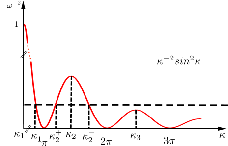
Figure 2: Dependence of $\kappa$ on $\omega$.

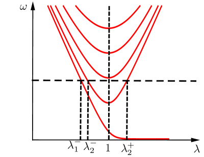
Figure 3: Energy bands for zigzag graphene nanoribbon. Dependence of wave vector $\lambda$ on energy $\omega$.

(1) $0<\omega<1$. Equation (11) has a solution $\kappa=i\tau$ where $\tau$ is real and satisfies

$$\frac{\sinh\tau}{\tau}=\pm\frac{1}{\omega}.$$

Then $\lambda=\tau\coth\tau$ and

$$\mathcal{U}(x)=i\sinh(\tau x)\ ,\ \ \mathcal{V}(x)=\mp\sinh(\tau(x-1))$$

(2) $\omega=1$. The solution to (11) is $\kappa=0$, $\lambda=1$ and the vector $(U,\mathcal{V})$ is given by (9).

(3) $\omega>1$. Then $\kappa$ is real and satisfies (11) and corresponding $\lambda$ is evaluated by (12). In order to describe solutions of (11) the real numbers $\kappa_{j}$ are introduced as the maximum of $\kappa^{-2}sin^{2}\kappa$ on the interval $[(j-1)\pi,\,j\pi)$, $j=1,2,\ldots$ (see Figure 2). We put

$$\frac{1}{\omega_{j}^{2}}=\frac{\sin^{2}\kappa_{j}}{\kappa_{j}^{2}},\;\;\text{and note that}\qquad\frac{d}{d\kappa}\Big{(}\frac{\sin^{2}\kappa}{\kappa^{2}}\Big{)}\Big{|}_{\kappa=\kappa_{j}}=0.$$

Then $\lambda_{j}=1\>\text{and}\>\kappa_{j}=\sqrt{\omega_{j}^{2}-1}.$ From (11) it follows that $\omega_{j}$ satisfies

$$\frac{\omega^{2}-1}{\omega^{2}}=\sin^{2}(\sqrt{\omega^{2}-1}).$$ (14)

One can verify that $\kappa_{j}<(2j-1)\pi/2$ and $\kappa_{1}=0$, $\omega_{1}=1$. (a) If $\omega\in(\omega_{N-1},\omega_{N})$, $N=2,\,3\ldots$, then there are $2N-3$ solutions with real $\lambda$, which can be labelled as follows (see Figure 2 and Figure 3)

$$\lambda_{j}^{\pm}=\kappa_{j}^{\pm}\cot(\kappa_{j}^{\pm}),\>\>\>j=2,\,3,\ldots,\,N-1,$$

where $\kappa_{j}^{\pm}\in((j-1)\pi,j\pi)$ satisfies

$$\frac{\sin\kappa_{j}^{\pm}}{(\kappa_{j}^{\pm})}=\frac{(-1)^{j+1}}{\omega}\;\;\mbox{and $\kappa_{j}^{+}<\kappa_{j}<\kappa_{j}^{-}$}.$$

The corresponding solutions to (5) are given by

$$w_{j}^{\pm}(x,y)=e^{-i\lambda_{j}^{\pm}y}(\mathcal{U}_{j}^{\pm}(x),\mathcal{V}_{j}^{\pm}(x)),$$ (15)

where

$$(\mathcal{U}_{j}^{\pm}(x),\mathcal{V}_{j}^{\pm}(x))=(\sin(\kappa_{j}^{\pm}x),(-1)^{j+1}i\sin(\kappa_{j}^{\pm}(x-1))).$$ (16)

There is only one solution of (11) labeled by a negative index $"-"$ on the interval $(0,\pi)$, which we denote by $\kappa_{1}^{-}$ and corresponding value of $\lambda$ by $\lambda_{1}^{-}$. The corresponding solution $(\mathcal{U},\mathcal{V})$ is given by $w_{1}^{-}(x,y)=e^{-i\lambda_{1}^{-}y}(\mathcal{U}_{1}^{-}(x),\mathcal{V}_{1}^{-}(x))$, where $\mathcal{U}_{1}^{-}$ and $\mathcal{V}_{1}^{-}$ are evaluated by (16) with $j=1$. (b) The case $\omega=\omega_{N}$, $N\geq 2$, is called the threshold case. Here we have $2N-3$ solutions, described already in the case (a). In addition there are two solutions with $\lambda=1$ and $\kappa=\kappa_{N}$, which have the form

$$w_{N}^{0}(x,y)=e^{-iy}(\sin(\kappa_{N}x),(-1)^{N+1}i\sin(\kappa_{N}(x-1)))$$ (17)

and

$$w_{N}^{1}(x,y) =yw_{N}^{0}(x,y)-\kappa_{N}^{-1}e^{-iy}(ix\cos(\kappa_{N}x),(-1)^{N+1}(1-x)\cos(\kappa_{N}(x-1))),$$ (18)

where the last solution has linear growth in $y$.

Thus for each $\omega\in(0,\infty)$ there exists a bounded solution to (5), (4) of the form (15). Hence the continuous spectrum of the Dirac operator ${\mathcal{D}}$ is the whole real line, i.e.

$$\sigma_{c}=\mathbb{R}.$$

2.4 Solutions of the form (7) with non-real wave vector $\lambda$

We will see in what follows that trapped modes may be generated by solutions to (5), (4) with non-real $\lambda$. In this section we describe such solutions with $\lambda$ close to the real axis.

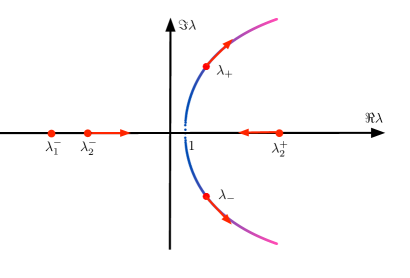
Figure 4: Bifurcation of $\lambda$ from the threshold.

Consider the case when $\omega$ is close to $\omega_{N}$, $N=2,\,3,\ldots$ We introduce a small positive parameter $\varepsilon$ and denote by $\omega_{\varepsilon}$ the energy satisfying $\omega_{\varepsilon}^{-1}=\omega_{N}^{-1}+\varepsilon$. Then the double root $\lambda=1$ of (12) with $\omega=\omega_{N}$ bifurcates into two roots $\lambda_{\pm}=\lambda_{\pm}(\varepsilon)$ (see Figure 4). These roots can be found from the equation

$$g(\lambda,\varepsilon)=\frac{(-1)^{N+1}}{\omega_{\varepsilon}},\;\;g(\lambda,\varepsilon)=\frac{\sin\sqrt{\omega_{\varepsilon}^{2}-\lambda^{2}}}{\sqrt{\omega_{\varepsilon}^{2}-\lambda^{2}}}.$$ (19)

From the definition (19), it follows that $g(\lambda,\varepsilon)$ is an analytic function of $(\omega_{\varepsilon}^{2}-\lambda^{2})$. Using Taylor’s formula for the function $g$ near the point $(\lambda,\varepsilon)=(1,0)$, we get

$$g(\lambda,\varepsilon)-\frac{(-1)^{N+1}}{\omega_{N}}=(-1)^{N}\Big{(}\varepsilon+\frac{(\lambda-1)^{2}}{2\omega_{N}(\omega_{N}^{2}-1)}+\frac{\omega_{N}^{2}(\lambda-1)\varepsilon}{\omega_{N}^{2}-1}$$

$$+\frac{(2+3\omega_{N}^{2})(\lambda-1)^{3}}{6\omega_{N}(\omega_{N}^{2}-1)^{2}}\Big{)}+O(|\lambda-1|^{4}+|\lambda-1|^{2}\varepsilon+\varepsilon^{2}).$$ (20)

By means of (20) one can find the expansions

$$\lambda_{\pm}=1\pm\sqrt{\varepsilon}\lambda_{1}i+\varepsilon\lambda_{2}+O(\varepsilon^{3/2}),$$ (21)

where $\lambda_{1}=\sqrt{2\omega_{N}(\omega_{N}^{2}-1)}$ and $\lambda_{2}=2\omega_{N}/3$. Since $\overline{g(\lambda,\varepsilon)}=g(\overline{\lambda},\varepsilon)$, it follows that $\overline{\lambda_{+}}=\lambda_{-}$. Then, from the energy relation $\lambda_{\pm}^{2}+\kappa_{\pm}^{2}=\omega_{\varepsilon}^{2}$, we find

$$\kappa_{\pm}=\kappa_{N}\mp\sqrt{\varepsilon}\kappa_{N1}i+O(\varepsilon)$$ (22)

where $\kappa_{N}=\sqrt{\omega_{N}^{2}-1}$ and $\kappa_{N1}=2\sqrt{\omega_{N}}$. Now, solutions to (5), (4) of the form (7) with $\lambda_{\pm}$ are given by

$$w_{N}^{\pm}(x,y)=e^{-i\lambda_{\pm}y}\left(\begin{array}[]{c}\sin(\kappa_{\pm}x)\\ (-1)^{N+1}i\sin(\kappa_{\pm}(x-1))\end{array}\right)$$ (23)

and by (21) and (22) it can be written in terms of $w_{0}^{N}$ and $w_{1}^{N}$ (see (17) and (18)) as

$$w_{N}^{\pm}(x,y)=w_{0}^{N}\pm\sqrt{\varepsilon}\sqrt{2\omega_{N}(\omega_{N}^{2}-1)}w_{1}^{N}+O(\varepsilon).$$ (24)

Waves (23) are not analytic in $\varepsilon$. Consider instead their linear combinations

$$\mathbf{w}_{N}^{\varepsilon+}(x,y) =\frac{1}{2\pi i}\int\limits_{|\lambda-1|=a}\frac{e^{-i\lambda y}}{g(\lambda,\varepsilon)-(-1)^{N+1}\omega_{\varepsilon}^{-1}}\left(\begin{array}[]{c}\sin(\kappa(\lambda)x)\\ (-1)^{N+1}i\sin(\kappa(\lambda)(x-1))\end{array}\right)d\lambda$$ (27)

$$=\gamma_{+}^{\varepsilon}w_{N}^{+}+\gamma_{-}^{\varepsilon}w_{N}^{-},$$ (28)

and

$$\mathbf{w}_{N}^{\varepsilon-}(x,y) =\frac{1}{2\pi i}\int\limits_{|\lambda-1|=a}\frac{(\lambda-1)e^{-i\lambda y}}{g(\lambda,\varepsilon)-(-1)^{N+1}\omega_{\varepsilon}^{-1}}\left(\begin{array}[]{c}\sin(\kappa(\lambda)x)\\ (-1)^{N+1}i\sin(\kappa(\lambda)(x-1))\end{array}\right)d\lambda$$ (31)

$$=\gamma_{+}^{\varepsilon}(\lambda_{+}-1)w_{N}^{+}+\gamma_{-}^{\varepsilon}(\lambda_{-}-1)w_{N}^{-},$$ (32)

where $\kappa(\lambda)=\sqrt{\omega^{2}-\lambda^{2}}$ and

$$\gamma_{\pm}^{\varepsilon}=\Big{(}{\frac{\partial g}{\partial\lambda}(\lambda_{\pm},\varepsilon)}\Big{)}^{-1},$$ (33)

one can verify that $\gamma_{-}^{\varepsilon}=\overline{\gamma_{+}^{\varepsilon}}$. Here $a$ is such that the disc $\{|\lambda-1|\leq a\}$ contains exaclty two solutions $\lambda_{+}$ and $\lambda_{-}$ to (19). Above waves are analytic in $\varepsilon$ because the function $(g(\lambda,\varepsilon)-(-1)^{N+1}\omega_{\varepsilon}^{-1})^{-1}$ is analytic in $\varepsilon$ for $\lambda$ satisfying $|\lambda-1|=a$.

Now let us consider waves (28) and (32) in the limit case $\varepsilon=0$. First from (20) we obtain the following expansion $\frac{\partial g}{\partial\lambda}$ near the point $(\lambda,\varepsilon)=(1,0)$

$$\frac{\partial g}{\partial\lambda}(\lambda,\varepsilon)=(-1)^{N}(\frac{\lambda-1}{\omega_{N}(\omega_{N}^{2}-1)}+\frac{\omega_{N}^{2}\varepsilon}{(\omega_{N}^{2}-1)}+\frac{(2+3\omega_{N}^{2})(\lambda-1)^{2}}{2\omega_{N}(\omega_{N}^{2}-1)^{2}}\Big{)}+O(|\lambda-1|^{3}+|\lambda-1|\varepsilon).$$ (34)

From (33) and (34) combined with (21), we get the following expansion

$$\gamma_{\pm}^{\varepsilon}=(-1)^{N}\frac{\sqrt{\omega_{N}(\omega_{N}^{2}-1)}}{\sqrt{\varepsilon}\sqrt{2}i}\Big{(}\pm 1+i\sqrt{\varepsilon}\frac{\sqrt{\omega_{N}}(-3\omega_{N}^{2}+\omega_{N}-\frac{4}{3})}{\sqrt{2(\omega_{N}^{2}-1)}}\Big{)}+O(\sqrt{\varepsilon}).$$ (35)

Finally, combining (24) with (35), we get

$$\mathbf{w}_{N}^{\varepsilon+}=\tilde{A}w_{0}^{N}-i\tilde{B}w_{1}^{N}+O(\varepsilon)$$

and

$$\mathbf{w}_{N}^{\varepsilon-}=\tilde{B}w_{0}^{N}+O(\varepsilon),$$

where $\tilde{A}$ and $\tilde{B}$ are real constants given by

$$\tilde{A}=(-1)^{N+1}2\omega_{N}^{2}(\omega_{N}^{2}-1)(2\omega_{N}^{2}+\frac{4}{3}),\>\>\>\tilde{B}=(-1)^{N}2\omega_{N}(\omega_{N}^{2}-1).$$

2.5 Location of the wave vector $\lambda$

The forthcoming analysis, which is based on the Laplace transform of the problem (5), (4) with respect to $y$, requires a knowledge of location of roots to equation (11), (12) or equivalently of the equation

$$\cos\kappa-\lambda\frac{\sin\kappa}{\kappa}=0,\;\;\kappa^{2}=\omega^{2}-\lambda^{2}.$$ (36)

Let us denote the left-hand side of (36) by $\mathcal{F}(\lambda)$, which is analytic with respect to $\lambda$. One can verify that

$$\frac{d}{d\lambda}\mathcal{F}(\lambda)=\frac{\lambda^{2}}{\kappa^{2}}\mathcal{F}(\lambda)+\frac{\omega^{2}(\lambda-1)}{\kappa^{2}}\frac{\sin\kappa}{\kappa},\;\;\;\kappa=\sqrt{\omega^{2}-\lambda^{2}}.$$

We collect required properties of the roots in the following

Proposition 1.

(i) All roots $\lambda$ of (36) are simple except of the case $\omega>1$ and $\omega$ is at the threshold - it is a root of (14). In this case the root $\lambda=1$ is double and all the other roots are simple.

(ii) Let $\omega>1$. Then there exists an absolute constant $c_{0}$ such that the set $S=\{\lambda=a+ib\,:\,|a|\geq c_{0}\omega,\;\;|b|\leq|a|\}$ contains no roots of (36).

(iii) Let $\omega_{\varepsilon}^{-1}=\omega_{k}^{-1}+\varepsilon$ for a certain $k=2,\,3,\ldots$, then there exist $\gamma_{k}>0$ and $\varepsilon_{k}>0$ such that for $\varepsilon\in(0,\varepsilon_{k}]$ all solutions to (36) which are located in the strip $|\Im\lambda|\leq\gamma_{k}$ are real described in Sect. 2.3 and complex described in Sect. 4 .

Proof.

(i) Assume that $F(\lambda)=\frac{d}{d\lambda}\mathcal{F}(\lambda)=0$. Consider two cases $\lambda\neq 1$ and $\lambda=1$. In the first case $\kappa\neq 0$ and $\sin\kappa=0$, which due to the first equation in (36) leads to $\cos\kappa=0$ what is impossible. Consider the second case $\lambda=1$. Then $\mathcal{F}(1)=0$, $\kappa^{2}=\omega^{2}-1$ and $\omega>1$ solves (14).

(ii) Let $\lambda=a+bi\in S$. Then $\kappa=i\lambda(1+O(\omega^{2}\,|\lambda|^{-2}))$. Since $|\sin\kappa|^{2}=\cosh^{2}\Im\kappa-\cos^{2}\Re\kappa$, we have

$$|\sin\kappa|^{2}-\frac{1}{\omega^{2}}|\kappa|^{2}\geq\cosh^{2}\Im\kappa-1-(1+|a|)^{2}-|a|^{2},$$

which implies the required assertion.

(iii) Due to (ii) it is sufficient to prove that there are no roots on the intervals where $\lambda=a\pm i\gamma$ and $|a|\leq C$, where $C$ is a certain positive constant. We can assume that $\gamma\leq 1$. First, we note that

$$\frac{sin\kappa}{\kappa}-\frac{(-1)^{k+1}}{\omega_{\varepsilon}}=g(\lambda,\varepsilon)-\frac{(-1)^{k+1}}{\omega_{\varepsilon}}=\Big{(}g(a,0)-\frac{(-1)^{k+1}}{\omega_{k}}\Big{)}\pm i\gamma\frac{\partial g}{\partial\lambda}(a,0)+O(\gamma^{2}+\varepsilon).$$

If $a\in[-C,1-\delta]\cup[1+\delta,C]$, then $\Big{(}g(a,0)-\frac{(-1)^{k+1}}{\omega_{k}}\Big{)}$ and $\frac{\partial g}{\partial\lambda}(a,0)$ are real and

$$c(\delta,C)=\max_{[-C,1-\delta]\cup[1+\delta,C]}\Big{(}|g(a,0)-\frac{(-1)^{k+1}}{\omega_{k}}|+\Big{|}\frac{\partial g}{\partial\lambda}(a,0)\Big{|}\Big{)}|>0.$$

Furthermore,

$$|g(\lambda,\varepsilon)-\frac{(-1)^{k+1}}{\omega_{\varepsilon}}|\geq|\gamma|c(\delta,C)-C_{1}(\gamma^{2}+\varepsilon).$$

Consider $\lambda$ close to $1$. More exactly, let $|\Im\lambda|=\delta$ and $|a-1|\leq\delta$. Noting that $g(1,0)-\frac{(-1)^{k+1}}{\omega_{k}}=\frac{\partial g}{\partial\lambda}(1,0)=0$ and using representation (20), we get

$$g(\lambda,\varepsilon)-\frac{(-1)^{k+1}}{\omega_{\varepsilon}}=(-1)^{N}\frac{(\lambda-1)^{2}}{2\omega_{k}^{2}(\omega_{k}-1)}+O(\delta^{3}+\varepsilon).$$

Since $|\lambda-1|^{2}\geq\delta^{2}$, we conclude from the last estimate that there are positive constants $c_{1}$ and $c_{2}$ depending only on $k$ such that, if $\delta\leq c_{1}$ and $\varepsilon\leq c_{2}\delta^{2}$, then $g(\lambda,\varepsilon)-\frac{(-1)^{k+1}}{\omega_{\varepsilon}}$ does not vanish on the intervals $|\Im\lambda|=\delta$, $|a-1|\leq\delta$. ∎

2.6 Symplectic form

There is a natural symplectic structure on the set of solutions to problem (5), (4), cf. [17, Ch. 5]. It will play important role in the study of the scattering matrix.

For two solutions $w=(u,v)$ and $\tilde{w}=(\tilde{u},\tilde{v})$ of the problem (5), (4), let us define the quantity

$$q_{a}(w,\tilde{w})=-\int_{0}^{1}(u(x,a)\overline{\tilde{v}(x,a)}-v(x,a)\overline{\tilde{u}(x,a)})dx.$$ (37)

Since

$$0=\int_{\Pi_{a,b}}\left(\begin{array}[]{c}\overline{\tilde{u}}\\ \overline{\tilde{v}}\end{array}\right)\cdot({\mathcal{D}}-\omega I)\left(\begin{array}[]{c}u\\ v\end{array}\right)dxdy-\int_{\Pi_{a,b}}\left(\begin{array}[]{c}u\\ v\end{array}\right)\cdot(\overline{\mathcal{D}}-\omega I)\left(\begin{array}[]{c}\overline{\tilde{u}}\\ \overline{\tilde{v}}\end{array}\right)dxdy\\ =q_{b}(w,\tilde{w})-q_{a}(w,\tilde{w}),$$

where $\Pi_{a,b}=(0,1)\times(a,b)$, $a<b$, we see that $q_{a}$ does not depend on $a$ and we will use the notation q for this form.
The form q is sesquilinear

$$q(\alpha_{1}w_{1},\alpha_{2}w_{2})=\alpha_{1}\overline{\alpha_{2}}q(w_{1},w_{2})$$

and anti-Hermitian

$$\overline{q(w_{1},w_{2})}=-q(w_{2},w_{1})$$

hence it is symplectic.

2.7 Biorthogonality conditions

Here we discuss the biorthogonality conditions for solutions to (5), (4). Since we are interested mostly in the case when $\omega=\omega_{\varepsilon}$, where $\omega_{\varepsilon}^{-1}=\omega_{N}^{-1}+\varepsilon$ , we will consider this case here. We introduce solutions to (5), (4) as follows

$$w_{j}^{\tau}(x,y)=e^{-i\lambda_{j}^{\tau}y}(\mathcal{U}_{j}^{\tau}(x),\mathcal{V}_{j}^{\tau}(x)),$$ (38)

where $\tau$ stands for $+$ or $-$ and $j=1,\ldots,N$ (if $j=1$, then only $\tau=-$ is admissible). Furthermore, if $j=1,\ldots,N-1$, then the functions $\mathcal{U}_{j}^{\tau}$ and $\mathcal{V}_{j}^{\tau}$ are given by (16) and in the case $j=N$ they are given by (23). Since

$$q_{a}(w_{j}^{\tau},w_{k}^{\theta})=e^{-i(\lambda_{j}^{\tau}-\overline{\lambda_{k}^{\theta}})a}C_{jk}^{\tau\theta},$$

where $C_{jk}^{\tau\theta}$ is a constant, and since the form $q$ is independent of $a$, we conclude that

$$q(w_{j}^{\tau},w_{k}^{\theta})=0\;\;\mbox{if $(j,\tau)\neq(k,\theta)$\;\;\mbox{and $q(w_{j}^{\tau},w_{j}^{\tau})=\frac{i}{\omega}(\lambda_{j}^{\tau}-1)$}}.$$

Therefore,

$$q(w_{j}^{\tau},w_{k}^{\theta})=\frac{i}{\omega}(\lambda_{k}^{\tau}-1)\delta_{j,k}\delta_{\tau,\theta}$$ (39)

for $j,k=1,\ldots,N-1$ and $\tau,\theta=\pm$.

Let us start with the oscillatory waves. We put

$${\bf w}_{k}^{\tau}=\frac{\sqrt{\omega}}{\sqrt{|\lambda_{k}^{\tau}-1|}}w_{k}^{\tau},\;\;\;k=1,\ldots,N-1.$$

Then by (39)

$$q({\bf w}_{j}^{\tau},{\bf w}_{k}^{\theta})=\tau i\delta_{j,k}\delta_{\tau,\theta},\,\tau,\theta=\pm.$$ (40)

In the case $\omega=\omega_{N}$, we have

$$q(w_{N}^{0},w_{N}^{0})=0,\ q(w_{N}^{0},w_{N}^{1})=\frac{1}{2\omega_{N}},\;q(w_{N}^{1},w_{N}^{1})=\frac{i}{6\omega_{N}(\omega_{N}^{2}-1)},$$

for waves (17), (18).

2.8 Biorthogonality conditions for the complex wave vector $\lambda$

Let us check if the waves $\mathbf{w}_{N}^{\varepsilon\pm}$ fullfil orthogonality conditions. For waves $w_{N}^{\pm}$ we have

$$q(w_{N}^{\pm},w_{N}^{\pm})=0,\ \ \ q(w_{N}^{+},w_{N}^{-})=\frac{i}{\omega}(\lambda_{+}-1),\ \ \ q(w_{N}^{-},w_{N}^{+})=\frac{i}{\omega}(\lambda_{-}-1).$$ (41)

We put

$$a^{\varepsilon}:=iq(\mathbf{w}_{N}^{\varepsilon+},\mathbf{w}_{N}^{\varepsilon+}),\quad b^{\varepsilon}:=-iq(\mathbf{w}_{N}^{\varepsilon+},\mathbf{w}_{N}^{\varepsilon-}),\quad c^{\varepsilon}:=-iq(\mathbf{w}_{N}^{\varepsilon-},\mathbf{w}_{N}^{\varepsilon-})$$ (42)

Then using (41) together with (28), (32) and (35) we obtian

$$a^{\varepsilon}\rightarrow a^{0}:=2\omega_{N}(\omega_{N}^{2}-1)\frac{5+9\omega_{N}^{2}}{3},$$ (43)

$$b^{\varepsilon}\rightarrow b^{0}:=2\omega_{N}(\omega_{N}^{2}-1)^{2},$$ (44)

$$c^{\varepsilon} =\varepsilon 4\omega_{N}(\omega_{N}^{2}-1)^{2}\frac{9\omega_{N}^{2}-3\omega_{N}+7}{3}+O(\varepsilon^{2})\>\>\mbox{as}\>\>\varepsilon\rightarrow 0$$

The functions $a^{\varepsilon}$, $b^{\varepsilon}$ and $c^{\varepsilon}$ are real and analytic, and $a^{\varepsilon},b^{\varepsilon},c^{\varepsilon}>0$ for small $\varepsilon>0$.

From the above evaluations we see that waves $\mathbf{w}_{N}^{\varepsilon+}$ and $\mathbf{w}_{N}^{\varepsilon-}$ do not fullfil the biorthogonality conditions. That is why we consider their linear combinations

$${\bf w}_{N}^{+}=\frac{\mathbf{w}_{N}^{\varepsilon+}+\alpha_{\varepsilon}\mathbf{w}_{N}^{\varepsilon-}}{N_{1}^{\varepsilon}},\;\;\;{\bf w}_{N}^{-}=\frac{\mathbf{w}_{N}^{\varepsilon+}}{N_{2}^{\varepsilon}}$$ (45)

where $\alpha_{\varepsilon}$ is unknown constant and $N_{1}^{\varepsilon}$ and $N_{2}^{\varepsilon}$ are normalizing factors.

Our aim is to fulfil the biorthogonality relations

$$q({\bf w}_{N}^{\tau},{\bf w}_{N}^{\theta})=\tau i\delta_{\tau,\theta},\,\tau,\theta=\pm,$$ (46)

which implies, in particular, that

$$q(\mathbf{w}_{N}^{\varepsilon+},\mathbf{w}_{N}^{\varepsilon+})+\alpha_{\varepsilon}q(\mathbf{w}_{N}^{\varepsilon-},\mathbf{w}_{N}^{\varepsilon+})=0.$$

Therefore, using (42), (43) and (44), we get

$$\alpha_{\varepsilon}=\frac{a^{\varepsilon}}{b^{\varepsilon}}=\frac{a^{0}}{b^{0}}+O(\varepsilon).$$

From (46) and (42), we find also the normalization factors $N_{1}^{\varepsilon}$ and $N_{2}^{\varepsilon}$

$$N_{1}^{\varepsilon}=\sqrt{a^{0}}+O(\varepsilon)\quad N_{2}^{\varepsilon}=\sqrt{a^{\varepsilon}}=\sqrt{a^{0}}+O(\varepsilon)$$

By (28), (32) and (45), we have

$${\bf w}_{N}^{+}=\alpha_{1}w_{N}^{+}+\beta_{1}w_{N}^{-}$$ (47)

and

$${\bf w}_{N}^{-}=\alpha_{2}w_{N}^{+}+\beta_{2}w_{N}^{-},$$ (48)

where

$$\alpha_{1}=\frac{\gamma_{+}^{\varepsilon}(1+\alpha_{\varepsilon}(\lambda_{+}-1))}{N_{1}^{\varepsilon}},\,\beta_{1}=\frac{\gamma_{-}^{\varepsilon}(1+\alpha_{\varepsilon}(\lambda_{-}-1))}{N_{1}^{\varepsilon}}$$ (49)

and

$$\alpha_{2}=\frac{\gamma_{+}^{\varepsilon}}{N_{2}^{\varepsilon}},\,\beta_{2}=\frac{\gamma_{-}^{\varepsilon}}{N_{2}^{\varepsilon}}.$$ (50)

Then biorthogonality conditions take the form (46).

2.9 Properties of coefficients (49) and (50)

Accoriding to definitions (49) and (50), one can check that

$$\overline{\beta_{1}}=\alpha_{1},\;\;\;\overline{\beta_{2}}=\alpha_{2}.$$ (51)

In the next proposition, we collect some more properties of coefficients (49) and (50), which will play an important role in the sequel.

Proposition 2.

The following relations hold

$$\frac{\alpha_{1}}{\alpha_{2}}=\frac{\beta_{2}}{\beta_{1}},\;\;\;\;\;\;\;\Big{|}\frac{\alpha_{1}}{\alpha_{2}}\Big{|}=1.$$ (52)

Proof.

From (46) it follows

$$\alpha_{1}\overline{\beta_{1}(}\lambda_{+}-1)+\beta_{1}\overline{\alpha_{1}(}\lambda_{-}-1)=\omega,\;\;\;\;\;\\ \alpha_{2}\overline{\beta_{2}(}\lambda_{+}-1)+\beta_{2}\overline{\alpha_{2}(}\lambda_{-}-1)=-\omega,$$ (53)

and

$$\alpha_{1}\overline{\beta_{2}(}\lambda_{+}-1)+\beta_{1}\overline{\alpha_{2}(}\lambda_{-}-1)=0,$$ (54)

Eliminating $\omega$ from (53), we get

$$\frac{\lambda_{-}-1}{\lambda_{+}-1}=-\frac{\alpha_{1}\overline{\beta_{1}}+\alpha_{2}\overline{\beta_{2}}}{\beta_{1}\overline{\alpha_{1}}+\beta_{2}\overline{\alpha_{2}}}=-\frac{\alpha_{1}^{2}+\alpha_{2}^{2}}{\overline{\alpha_{1}^{2}}+\overline{\alpha_{2}^{2}}}$$

where the last equality follows form (51). Inserting it into (54), we arrive at

$$\alpha_{1}\alpha_{2}-\overline{\alpha_{1}}\overline{\alpha_{2}}\frac{\alpha_{1}^{2}+\alpha_{2}^{2}}{\overline{\alpha_{1}^{2}}+\overline{\alpha_{2}^{2}}}=0.$$ (55)

Dividing (55) by $\alpha_{2}(\overline{\alpha_{2}})^{2}$ and multiplying by $\overline{\alpha_{1}^{2}}+\overline{\alpha_{2}^{2}}$, we obtain

$$\frac{\alpha_{1}}{\alpha_{2}}+\frac{\alpha_{1}}{\alpha_{2}}(\frac{\overline{\alpha_{1}}}{\overline{\alpha_{2}}})^{2}-\frac{\overline{\alpha_{1}}}{\overline{\alpha_{2}}}(\frac{\alpha_{1}}{\alpha_{2}})^{2}-\frac{\overline{\alpha_{1}}}{\overline{\alpha_{2}}}=0.$$

Defining $d=\alpha_{1}/\alpha_{2}$ , this relation can be written as

$$(d-\overline{d})(1-d\overline{d})=0.$$

Here $d\neq\overline{d}$ because otherwise $\lambda_{+}$ would be real, this follows from the definitions of $\alpha_{1}$ and $\alpha_{2}$. Consequently

$$(1-d\overline{d})=0,\,\,\,|d|=1,$$ (56)

which implies the second equality in (52). To prove first equality in (52) we note that $d=\alpha_{1}/\alpha_{2}=\overline{\beta_{1}}/\overline{\beta_{2}}$ by (51). This together with (56) gives

$$1-\frac{\alpha_{1}}{\alpha_{2}}\frac{\beta_{1}}{\beta_{2}}=0,\,\,\,\frac{\alpha_{1}}{\alpha_{2}}=\frac{\beta_{2}}{\beta_{1}}.$$

The proof is completed. ∎

The following quantity will play an important role

$$d=d(\varepsilon):=\frac{\alpha_{1}}{\alpha_{2}}=\frac{\beta_{2}}{\beta_{1}},$$ (57)

where the last equality is borrowed from Proposition 2. By (56), the absolute value of $d$ is equal to $1$. Moreover the function $d(\varepsilon)$ depends on $\varepsilon\in[0,\varepsilon_{0}]$ and by definitions of
$\alpha_{1}$ and $\alpha_{2}$, see (49) and (50)

$$d(\varepsilon)=1+i\frac{(5+9\omega_{N}^{2})}{3}\sqrt{\frac{2\omega_{N}}{\omega_{N}^{2}-1}}\sqrt{\varepsilon}+O(\varepsilon).$$ (58)

We note also that

$$\mathbf{w}_{N}^{+}=Aw_{N}^{0}+iBw_{N}^{1}+O(\varepsilon)$$ (59)

and

$$\mathbf{w}_{N}^{-}=Cw_{N}^{0}+iBw_{N}^{1}+O(\varepsilon)$$ (60)

where

$$A=(-1)^{N}(-6\omega_{N}^{5}+2\omega_{N}^{3}+9\omega_{N}^{2}+4\omega_{N}+5)\sqrt{\frac{2\omega_{N}(\omega_{N}^{2}-1)}{3(9\omega_{N}^{2}+5)}},$$

$$B=(-1)^{N+1}\sqrt{\frac{6\omega_{N}(\omega_{N}^{2}-1)}{9\omega_{N}^{2}+5}},\>\>\>C=(-1)^{N+1}2\omega_{N}(3\omega_{N}^{2}+2)\sqrt{\frac{2\omega_{N}(\omega_{N}^{2}-1)}{3(9\omega_{N}^{2}+5)}}.$$

2.10 Non-homogeneous problem

Here, we consider the non-homogeneous problem

$$(-i\partial_{x}+\partial_{y})v-\omega u=g\;\;\;\mbox{in $\Pi$,}$$ (61)

$$(-i\partial_{x}-\partial_{y})u-\omega v=h\;\;\;\mbox{in\,\ $\Pi$,}$$ (62)

supplied with the boundary conditions

$$u(0,y)=0\;\;\mbox{and}\;\,v(1,y)=0,\;\;y\in\mathbb{R}.$$ (63)

To study solvability of this system, we introduce some spaces. The space $L_{\sigma}^{\pm}(\Pi)$, $\sigma>0$, consists of all functions $g$ such that $e^{\pm\sigma y}g\in L^{2}(\Pi)$. Furthermore,

$$X_{\sigma}^{\pm}=\{u\in L_{\sigma}^{\pm}(\Pi)\,:\,(i\partial_{x}+\partial_{y})u\in L_{\sigma}^{\pm}(\Pi),\;\;u(0,y)=0\},$$

$$Y_{\sigma}^{\pm}=\{v\in L_{\sigma}^{\pm}(\Pi)\,:\,(-i\partial_{x}+\partial_{y})v\in L_{\sigma}^{\pm}(\Pi),\;\;v(1,y)=0\}.$$

The norms in the above spaces are defined by $||g;L_{\sigma}^{\pm}(\Pi)||=||e^{\pm\sigma y}g;L^{2}(\Pi)||$,

$$||u;X_{\sigma}^{\pm}||=\Big{(}||u;L_{\sigma}^{\pm}(\Pi)||^{2}+||(i\partial_{x}+\partial_{y})u;L_{\sigma}^{\pm}(\Pi)||^{2}\Big{)}^{1/2}$$

and

$$||v;Y_{\sigma}^{\pm}||=\Big{(}||v;L_{\sigma}^{\pm}(\Pi)||^{2}+||(-i\partial_{x}+\partial_{y})v;L_{\sigma}^{\pm}(\Pi)||^{2}\Big{)}^{1/2}$$

respectively.

The main solvability result is the following assertion

Theorem 2.1.

Let $\omega>0$ and let $\sigma>0$ be such that the line $\Im\lambda=\pm\sigma$ contains no roots of (36). Then the operator

$$D-\omega I\;:\;X_{\sigma}^{\pm}\times Y_{\sigma}^{\pm}\;\to\;L_{\sigma}^{\pm}(\Pi)$$ (64)

is isomorphism.

Despite the problem, which we are dealing with is not elliptic the proof of this assertion is more or less standard and we present it in Appendix C.

In what follows we assume that an integer $N\geq 2$ is fixed, $\omega_{N}=\sqrt{\kappa_{N}^{2}+1}$, where $\kappa_{N}$ is defined in Sect. 2.3, and $\omega=\omega_{\varepsilon}=\omega_{N}/(1+\varepsilon\omega_{N})$. Then we have the following waves

$${\bf w}_{1}^{-},{\bf w}_{2}^{\pm},\ldots,{\bf w}_{N-1}^{\pm},{\bf w}_{N}^{\pm},$$

where ${\bf w}_{1}^{-}$ corresponding to $\lambda_{1}^{-}$ and ${\bf w}_{j}^{\pm}$, $j=2,\dots,N-1$ are oscillatory and ${\bf w}_{N}^{\pm}$ are of exponential growth.

Theorem 2.2.

Let $\gamma=\gamma_{N}$ and $\varepsilon_{N}$ be the same positive numbers as in Proposition 1 and also $(g,h)\in L_{\gamma}^{+}(\Pi)\cap L_{\gamma}^{-}(\Pi)$. Denote by $(u^{\pm},v^{\pm})\in X_{\gamma}^{\pm}\times Y_{\gamma}^{\pm}$ the solution of problem (61), (62), (63), which exist according to Theorem 2.1. Then

$$(u^{+},v^{+})=(u^{-},v^{-})+\sum_{j=2}^{N}C_{j}^{+}{\bf w}_{j}^{+}+\sum_{j=1}^{N}C_{j}^{-}{\bf w}_{j}^{-},$$ (65)

where

$$-iC_{j}^{+}=\int_{\Pi}\,(g,h)\cdot\overline{{\bf w}_{j}^{+}}dxdy,\;\;iC_{j}^{-}=\int_{\Pi}\,(g,h)\cdot\overline{{\bf w}_{j}^{-}}dxdy.$$

Proof of this Theorem is presented in Appendix D. Results similar to Theorems 2.1 and 2.2 are well-known for elliptic problems and can be found, for example, in [11], [12] and [17], but we remind that our problem is not elliptic, see Appendix A.

3 Dirac equation with potential

3.1 Problem statement

Here we examine the problem with a potential, prove solvability results and asymptotics formulas for solutions.
Consider the nanoribbon with a potential:

$${\mathcal{D}}\left(\begin{array}[]{c}u\\ v\end{array}\right)+\delta\mathcal{P}\left(\begin{array}[]{c}u\\ v\end{array}\right)=\omega\left(\begin{array}[]{c}u\\ v\end{array}\right),$$ (72)

$$u(0,y)=0\ ,\ \ v(1,y)=0,$$ (73)

where ${\mathcal{D}}$ is the same as in (5), $\mathcal{P}=\mathcal{P}(x,y)$ is a bounded, continuous and real-valued function with compact support in $\overline{\Pi}$ and $\delta$ is a small parameter. We assume in what follows that

$$\mbox{supp}\mathcal{P}\subset[-R_{0},R_{0}]\times[0,1]\>\>\>\mbox{and}\>\>\>\sup_{(x,y)\in\Pi}|\mathcal{P}(x,y)|\leq 1,$$ (74)

where $R_{0}$ is a fixed positive number.

We assume that positive numbers $\gamma$ and $\varepsilon_{N}$ are fixed such that

$$\omega=\omega_{\varepsilon}\;\;\;\mbox{where}\;\;\;\frac{1}{\omega_{\varepsilon}}=\frac{1}{\omega_{N}}+\varepsilon,\;N=2,\,3,\ldots,\;\;$$ (75)

$\varepsilon\in[0,\varepsilon_{N}]$ and $\gamma=\gamma_{N}$ is from Proposition 1(iii), i.e.

(1) the lines $\Im\lambda=\pm\gamma$ contain no roots of (36) with $\omega$ given by (75),

(2) the strip $|\Im\lambda|<\gamma$ contains roots of (36), which are real and complex described in Sect. 2.3 and 4 respectively.

Since the norm of the multiplication operator $\delta\mathcal{P}$ in $L^{2}(\Pi)$ is less than $\delta$ we derive from Theorem 2.1 the following assertion

Theorem 3.1.

The operator

$${\mathcal{D}}+(\delta\mathcal{P}-\omega_{\varepsilon})I\;:\;X_{\gamma}^{\pm}\times Y_{\gamma}^{\pm}\;\to\;L_{\gamma}^{\pm}(\Pi)$$ (76)

is isomorphism for $|\delta|\leq\delta_{0}$, where $\delta_{0}$ is a positive constant depending on the norm on the inverse operator $({\mathcal{D}}-\omega_{\varepsilon}I)^{-1}\,:\,L_{\gamma}^{\pm}(\Pi)\to L_{\gamma}^{\pm}(\Pi)$.

We introduce two new spaces

$${\mathcal{H}}_{\gamma}^{+}=\{(u,v)\;:\;u\in X_{\gamma}^{+}\cap X_{\gamma}^{-},\;\;v\in Y_{\gamma}^{+}\cap Y_{\gamma}^{-}\}$$

and

$${\mathcal{H}}_{\gamma}^{-}=\{(u,v)\;:\;u\in X_{\gamma}^{+}\cup X_{\gamma}^{-},\;\;v\in Y_{\gamma}^{+}\cup Y_{\gamma}^{-}\}.$$

The norms in this spaces are defined by

$$||(u,v);{\mathcal{H}}_{\gamma}^{\pm}||^{2}=\int_{\Pi}e^{\pm 2\gamma|y|}\Big{(}|u|^{2}+|v|^{2}+|{\mathcal{D}}(u,v)^{t}|^{2}\Big{)}dxdy.$$

Let also ${\mathcal{L}}_{\gamma}^{\pm},$ $\gamma>0$, be two $L^{2}$ weighted spaces in $\Pi$ with the norms

$$||(u,v);{\mathcal{L}}_{\gamma}^{\pm}||^{2}=\int_{\Pi}e^{\pm 2\gamma|y|}\Big{(}|u|^{2}+|v|^{2}\Big{)}dxdy.$$

We define two operators acting in the introduced spaces

$$A_{\gamma}^{\pm}=A_{\gamma}^{\pm}(\varepsilon,\delta)={\mathcal{D}}+(\delta\mathcal{P}-\omega)I\,:\,{\mathcal{H}}_{\gamma}^{\pm}\rightarrow{\mathcal{L}}_{\gamma}^{\pm}.$$

Some important properties of these operator are collected in the following

Theorem 3.2.

The operators $A_{\gamma}^{\pm}$ are Fredholm and ${\rm dim}\,{\rm ker}A_{\gamma}^{+}=0$, ${\rm dim}\,{\rm coker}\,A_{\gamma}^{-}=0$. Moreover

$${\rm dim}\,{\rm coker}A_{\gamma}^{+}={\rm dim}\,{\rm ker}A_{\gamma}^{-}=2N-1,$$

where $N$ is the same as in (75).

Proof.

By Theorem 3.1, the operator (76) is isomorphic. This implies that the operator $A_{\gamma}^{-}$ is surjective for such $\delta$ and its index and the dimension of his kernel does not depend on $\delta$ and hence equals $2N-1$ as it is in the case $\delta=0$.∎

In the next theorem and in what follows, we fix four smooth functions, $\chi_{\pm}=\chi_{\pm}(y)$ and $\eta_{\pm}=\eta_{\pm}(y)$ such that $\chi_{+}(y)=1$, $\chi_{-}(y)=0$ for $y>R_{0}$ and $\chi_{+}(y)=0$, $\chi_{-}(y)=1$ for $y<-R_{0}$. Then let $\eta_{\pm}(y)=1$ for large positive $\pm y$, $\eta_{\pm}(y)=0$ for large negative $\pm y$ and $\chi_{\pm}\eta_{\pm}=\chi_{\pm}$.

Let us derive an asymptotic formula for the solution to the perturbed problem (72), (73).

Theorem 3.3.

Let $f\in{\mathcal{L}}_{\gamma}^{+}$ and let $w=(u,v)\in{\mathcal{H}}_{\gamma}^{-}$ be a solution to

$$({\mathcal{D}}+(\delta\mathcal{P}-\omega)I)w=f.$$ (77)

satisfying (73).Then

$$w=\eta_{+}\sum_{j=1}^{N}\sum_{\tau=\pm}C_{j}^{\tau}{\bf w}_{j}^{\tau}+\eta_{-}\sum_{j=1}^{N}\sum_{\tau=\pm}D_{j}^{\tau}{\bf w}_{j}^{\tau}+R,$$ (78)

where $R\in{\mathcal{H}}_{\gamma}^{+}$ .

Proof.

We write (77) as

$$({\mathcal{D}}+\omega I)w=f-\delta\mathcal{P}w=:F$$

Then

$$({\mathcal{D}}+\omega I)\eta_{\pm}w=\eta_{\pm}F+[{\mathcal{D}},\eta_{\pm}]w.$$ (79)

According to Theorem 2.2 solutions to (79) are $w^{\mp}:=(u^{\mp},v^{\mp})\in X_{\gamma}^{\mp}\times Y_{\gamma}^{\mp}$, so

$$\eta_{+}w=w^{-},\>\>\>\eta_{-}w=w^{+}.$$ (80)

Applying relation (65) to (80), then multiplying obtained equations by $\chi_{\pm}$ respectively and summing them up, we get

$$w=\chi_{-}\sum_{j=1}^{N}\sum_{\tau=\pm}C_{j}^{{}^{\prime}\tau}{\bf w}_{j}^{\tau}+\chi_{+}\sum_{j=1}^{N}\sum_{\tau=\pm}D_{j}^{{}^{\prime}\tau}{\bf w}_{j}^{\tau}+R^{\prime}$$ (81)

where $R^{\prime}=\chi_{+}w^{+}+\chi_{-}w^{-}+(1-\chi_{+}-\chi_{-})w\in\mathcal{H_{\gamma}}^{+}$. Equation (81) can be written in the form (78) with $R\in\mathcal{H_{\gamma}}^{+}$.∎

3.2 Augumented scattering matrix

Scattering matrix is our main tool for the identification of trapped modes [20, 21, 22]. Using q-form, we define incoming/outgoing waves. Scattering matrix is defined via coefficients in this combination of waves. It is important to point out that this matrix is often called augumented as it contains coefficients of the waves exponentially growing at infinity as well. Finally, by the end of the section we define a space with separated asymptotics and check that it produces a unique solution to the perturbed problem.

Let

$$Q_{R}(w,\tilde{w})=q_{R}(w,\tilde{w})-q_{-R}(w,\tilde{w}).$$

If $w=(u,v)$ and $\tilde{w}=(\tilde{u},\tilde{v})$ are solutions to (5) for $|y|\geq R_{0}$ then using Green’s formula one can show that this form is independent of $R$, $R\geq R_{0}$.

We introduce two sets of waves with cutoff close to $\pm\infty$, which we will call outgoing and incoming (for physical interpretation see Appendix B)

$$W_{k}^{\mp}=W_{k}^{\mp}(x,y;\varepsilon)=\chi_{\pm}(y){\bf w}_{k}^{\mp}(x,y)$$ (82)

and

$$V_{k}^{\pm}=V_{k}^{\pm}(x,y;\varepsilon)=\chi_{\pm}(y){\bf w}_{k}^{\pm}(x,y)$$ (83)

with $k=2,\ldots,N$ for the sign $+$ and $k=1,\ldots,N$ for the sign $-$. The reason for introducing this sets of waves is the following property

$$Q_{R}(W_{k}^{\tau},W_{j}^{\theta})=-i\delta_{k,j}\delta_{\tau,\theta},\;\;Q_{R}(V_{k}^{\tau},V_{j}^{\theta})=i\delta_{k,j}\delta_{\tau,\theta}$$ (84)

where $k,j=2,\ldots,N$, $\tau,\theta=\pm$ and $k,j=1$, $\tau,\theta=-$. Moreover,

$$Q_{R}(W_{k}^{\tau},V_{j}^{\theta})=0.$$ (85)

Thus the sign of the $Q$-form distinguish among $W$ and $V$ waves.

In the next lemma we give a description of the kernel of the operator $A_{\gamma}^{-}$, which will be used in the definition of the scattering matrix.

Theorem 3.4.

There exists a basis in $\ker A_{\gamma}^{-}$ of the form

$$z_{k}^{\tau}=V_{k}^{\tau}+{\bf S}_{k\tau}^{1-}W_{1}^{-}+\sum_{\theta=\pm}\sum_{j=2}^{N}{\bf S}_{k\tau}^{j\theta}W_{j}^{\theta}+\tilde{z}_{k}^{\tau},$$ (86)

where $\tilde{z}_{k}^{\tau}\in{\mathcal{H}}_{\gamma}^{+}$. Moreover, the coefficients ${\bf S}_{k\tau}^{j\theta}={\bf S}_{k\tau}^{j\theta}(\varepsilon,\delta)$ are uniquely defined .

Proof.

Let $z\in\ker A_{\gamma}^{-}$. Since

$$({\mathcal{D}}-\omega)(\chi_{\pm}z)=-\delta\mathcal{P}\chi_{\pm}z+[{\mathcal{D}},\chi_{\pm}]z,$$

applying Theorem 2.2, we get

$$\chi_{\pm}z=\sum_{j=1}^{N}\sum_{\tau=\pm}a_{j\tau}^{\pm}{\bf w}_{j}^{\tau}+R_{\pm},\;\;R_{\pm}\in X_{\gamma}^{\pm}\times Y_{\gamma}^{\pm}.$$

Multiplying these equalities by $\chi_{\pm}$ and summing them up, we get

$$z=\sum_{j=1}^{N}\sum_{\tau=\pm}a_{j\tau}^{\pm}\chi_{\pm}{\bf w}_{j}^{\tau}+R,\;\;R=\chi_{+}R_{+}+\chi_{-}R_{-}+(1-\chi_{-}-\chi_{+})z\in{\mathcal{H}}_{\gamma}^{+}.$$

We write the last relation in the form

$$z=\sum_{j=1}^{N}\sum_{\tau=\pm}C_{j\tau}^{1}W_{j}^{\tau}+\sum_{j=1}^{N}\sum_{\tau=\pm}C_{j\tau}^{2}V_{j}^{\tau}+R,\;\;R\in{\mathcal{H}}_{\gamma}^{+}$$

and consider the map

$$\ker A_{\gamma}^{-}\ni z\mapsto\,\{C_{j\tau}^{2}\}\in\mathbb{C}^{2N-1},$$

which is linear and is denoted by ${\mathcal{J}}$. Let us show that it’s kernel is trivial. Indeed, if all $C_{j\tau}^{2}$ vanish, then

$$\int_{{}_{\Pi_{R}}}\overline{z}({\mathcal{D}}+(\delta\mathcal{P}-\omega)I)zdxdy=Q_{R}(z,z)\mapsto-i\sum|C_{j\tau}^{1}|^{2}\;\;\mbox{as $R\to\infty$,}$$

where $\Pi_{R}=(-R,R)\times(0,1)$. Hence $C_{j\tau}^{1}=0$, which leads to $z\in{\mathcal{H}}_{\gamma}^{+}$ and therefore $z=0$. This shows that the mapping ${\mathcal{J}}$ is invertible and we obtain existence of a basis in the form (86) together with uniqueness of coefficients ${\bf S}_{k\tau}^{j\theta}$. ∎

The matrix of coefficients ${\bf S}_{k\tau}^{j\theta}$ in (86) is called the scattering matrix (see the footnote on the previous page concerning $k=1$ and $j=1$).

3.3 Block notation

We shall use a vector notation

$${\bf W}=({\bf W}_{\bullet},{\bf W}_{\dagger}),{\bf\;\;\;V}=({\bf V}_{\bullet},{\bf V}_{\dagger}),$$

where

$${\bf W}_{\bullet}=(W_{1}^{-},W_{2}^{+},W_{2}^{-},\ldots,W_{N-1}^{+},W_{N-1}^{-}),\;\;\;{\bf W}_{\dagger}=(W_{N}^{+},W_{N}^{-})$$

and

$${\bf V}_{\bullet}=(V_{1}^{-},V_{2}^{+},V_{2}^{-},\ldots,V_{N-1}^{+},V_{N-1}^{-}),\;\;\;{\bf V}_{\dagger}=(V_{N}^{+},V_{N}^{-}).$$

Equation (86) in the vector form reads

$${\bf z}={\bf V}+{\bf S}{\bf W}+{\bf r}.$$ (87)

with

$${\bf z}=({\bf z}_{\bullet},{\bf z}_{\dagger})=(z_{1}^{-},z_{2}^{+},z_{2}^{-},..,z_{N-1}^{+},z_{N-1}^{-},z_{N}^{+},z_{N}^{-})\in{\mathcal{H}}_{\gamma}^{-},$$

$${\bf r}=({\bf r}_{\bullet},{\bf r}_{\dagger})=(r_{1}^{-},r_{2}^{+},r_{2}^{-},..,r_{N-1}^{+},r_{N-1}^{-},r_{N}^{+},r_{N}^{-})\in{\mathcal{H}}_{\gamma}^{+}$$

here both vectors ${\bf z}$ and $r$ has $2N-1$ elements. Matrix ${\bf S}={\bf S}(\varepsilon,\delta)$ is written blockwise

$$\mathcal{S}=\left(\begin{array}[]{cc}{\bf S}_{\bullet\bullet}&{\bf S}_{\bullet\dagger}\\ {\bf S}_{\dagger\bullet}&{\bf S}_{\dagger\dagger}\end{array}\right).$$

Relations (84) and (85) take the form

$$Q({\bf W},{\bf W})=-i\mathbb{I}\ ,\ \ Q({\bf V},{\bf V})=i\mathbb{I}\ \ \ Q({\bf W},{\bf V})=\mathbb{O}.$$ (88)

where $\mathbb{I}$ is the identity matrix and $\mathbb{O}$ is the null matrix.

Proposition 3.

The scattering matrix ${\bf S}$ is unitary.

Proof.

Since $z_{k}^{\tau}$ satisfies the homogeneous equation (73), by using the Green formula one can show that $Q({\bf z},{\bf z})=0$. Therefore

$$0=Q({\bf z},{\bf z})=Q({\bf V}+{\bf S}{\bf W},{\bf V}+{\bf S}{\bf W})=Q({\bf V},{\bf V})+Q({\bf S}{\bf W},{\bf S}{\bf W})=i\mathbb{I}-i{\bf S}^{*}{\bf S}$$

which proves the result.∎

Consider the non-homogeneous problem (77) with $f\in\mathcal{{L}}_{\gamma}^{+}(\Pi)$. This problem has a solution $w\in{\mathcal{H}}_{\gamma}^{-}$ which admits the asymptotic representation

$$w=\sum_{j=1}^{N}\sum_{\tau=\pm}C_{j\tau}^{1}W_{j}^{\tau}+\sum_{j=1}^{N}\sum_{\tau=\pm}C_{j\tau}^{2}V_{j}^{\tau}+R,\;\;R\in{\mathcal{H}}_{\gamma}^{+}$$ (89)

which is an rearrangement of the representation (78) This motivate the following definition of the space ${\mathcal{H}}_{\gamma}^{out}$ consisting of vector functions $w\in{\mathcal{H}}_{\gamma}^{-}$ which admits the asymptotic representation (89) with $C_{j\tau}^{2}=0$. The norm in this space is defined by

$$||w;{\mathcal{H}}_{\gamma}^{{\rm out}}||=(||R;{\mathcal{H}}_{\gamma}^{+}||^{2}+\sum_{j=1}^{N}\sum_{\tau=\pm}\,|C_{j\tau}^{1}|^{2})^{1/2}.$$

Now, we note that the kernel in Theorem 3.4 can be equivalently spanned by

$$Z_{k}^{\tau}=W_{k}^{\tau}+{\bf\tilde{S}}_{k\tau}^{1-}V_{1}^{-}+\sum_{\theta=\pm}\sum_{j=2}^{N}{\bf\tilde{S}}_{k\tau}^{j\theta}V_{j}^{\theta}+\tilde{Z}_{\text{}k}^{\tau},\>\>\>\tilde{Z}_{k}^{\tau}\in{\mathcal{H}}_{\gamma}^{+},$$ (90)

$\tilde{Z}_{k}^{\tau}\in{\mathcal{H}}_{\gamma}^{+}$, where the incoming and outgoing waves were interchanged (compare with (86)) and $\tilde{S}$ is a scattering matrix corresponding to that exchange.

Theorem 3.5.

For any $f\in\mathcal{L}_{\gamma}^{+}(\Pi)$, problem (77) has a unique solution $w\in{\mathcal{H}}_{\gamma}^{out}$ and the following estimate holds

$$||w;{\mathcal{H}}_{\gamma}^{{\rm out}}||\leq c||f;\mathcal{L}_{\gamma}^{+}(\Pi)||,$$ (91)

where the constant $c$ is independent of $\varepsilon\in[0,\varepsilon_{0}]$ and $|\delta|\leq\delta_{0}$. Moreover,

$$-iC_{j\tau}^{1}=\int_{\Pi}f\cdot\overline{Z_{j}^{\tau}}dxdy.$$ (92)

Proof.

Existence. According to Theorem 3.3 there exists a solution to (77) of the form (89). Subtracting a linear combination of the elements ${\bf z}_{j}^{\pm}$, we obtain a solution from ${\mathcal{H}}_{\gamma}^{out}$.

Uniqueness is proved in the same way as the isomorphism property of the mapping ${\mathcal{J}}$ in Theorem 3.4.

To prove (92) we multiply equation (77) by $\overline{Z_{j}^{\tau}}$and integrate over $\Pi_{R}=(-R,R)\times(0,1)$, that leads to

$$\int_{\Pi_{R}}f\cdot\overline{Z_{j}^{\tau}}dxdy=Q_{R}(w,Z_{j}^{\tau}),$$

where integration by parts is applied. Now using relation (90) and (88) and sending $R$ to infinity we arrive at (92). From representation (92) if follows that

$$|C_{j\tau}^{1}|\leq C_{\gamma}||f;\mathcal{L}_{\gamma}^{+}(\Pi)||.$$ (93)

Now estimate (91) follows from (93) combined with (89) where $C_{j\tau}^{2}=0$. From (89) the remainder $R\in{\mathcal{H}}_{\gamma}^{+}$ satisfies

$$({\mathcal{D}}+(\delta\mathcal{P}-\omega)I)R=F,$$

where $F:=f-\delta\mathcal{P}\sum_{j=1}^{N}\sum_{\tau=\pm}\Big{(}C_{j\tau}^{1}\chi_{\tau}{\bf w}_{j}^{-\tau}\Big{)}-\sum_{j=1}^{N}\sum_{\tau=\pm}\Big{(}C_{j\tau}^{1}[\mathcal{D},\chi_{\tau}]{\bf w}_{j}^{-\tau})$. Therefore, we get

$$||F;\mathcal{L}_{\gamma}^{+}(\Pi)|| \leq||f;\mathcal{L}_{\gamma}^{+}(\Pi)||+\sum_{j=1}^{N}\sum_{\tau=\pm}\Big{(}C_{j\tau}^{1}||\delta\mathcal{P}\chi_{\tau}{\bf w}_{j}^{-\tau}||\Big{)}$$

$$+\sum_{j=1}^{N}\sum_{\tau=\pm}\Big{(}C_{j\tau}^{1}||[\mathcal{D},\chi_{\tau}]{\bf w}_{j}^{-\tau}||\Big{)}\leq c||f;\mathcal{L_{\gamma}}^{+}(\Pi)||,$$ (94)

where the last inequality follows from (93). Moreover, it follows from Theorem (3.1) that

$$||R;L_{\gamma}^{\pm}(\Pi)||\leq c_{1}||F;L_{\gamma}^{\pm}(\Pi)||.$$ (95)

Combining (95) with (94), we get the estimate

$$||R;\mathcal{H}_{\gamma}^{+}(\Pi)||\leq c||f;\mathcal{L}_{\gamma}^{+}(\Pi)||,$$

∎

which together with (93) leads to (91).

3.4 Analyticity of the scattering matrix

We represent ${\bf S}$ as

$${\bf S}=\mathbb{I}+{\bf s},\;\;\;\mbox{or, equivalently,}\;\;{\bf S}_{j\tau}^{k\theta}=\delta_{k,j}\delta_{\tau,\theta}+{\bf s}_{j\tau}^{k\theta}.$$ (96)

Theorem 3.6.

The scattering matrix ${\bf S}(\varepsilon,\delta)$ depends analytically on small parameters $\varepsilon\in[0,\varepsilon_{0}]$ and $\delta\in[-\delta_{0},\delta_{0}]$. Moreover,

$${\bf s}_{j\tau}^{k\theta}=-i\delta\int_{\Pi}\,\mathcal{P}{\bf w}_{j}^{\tau}\cdot\overline{{\bf w}_{k}^{\theta}}dxdy+O(\delta^{2}).$$ (97)

Proof.

Consider the operator

$$A_{\gamma}^{out}(\varepsilon,0)\,:\,{\mathcal{H}}_{\gamma}^{out}\to\mathcal{L}_{\gamma}^{+}(\Pi).$$

Then it is isomorphism and

$$w=\Big{(}A_{\gamma}^{out}(\varepsilon,0)\Big{)}^{-1}f=\sum_{j=1}^{N}\sum_{\tau=\pm}C_{j\tau}^{1}W_{j}^{{\rm\tau}}+R=:U+R$$

is given by

$$C_{j\tau}^{1}(\varepsilon)=i\int_{\Pi}f\cdot\overline{{\bf w}_{j}^{\tau}}dxdy,\;\;R=\Big{(}A_{\gamma}^{+}(\varepsilon,0)\Big{)}^{-1}(f-({\mathcal{D}}-\omega)U).$$

We note that the vector function $({\mathcal{D}}-\omega)U$ has a compact support in $\overline{\Pi}$ and is analytic in $\varepsilon$. The coefficients $C_{j\tau}(\varepsilon)$ depend also analytically on $\varepsilon$. Thus the inverse operator $\Big{(}A_{\gamma}^{out}(\varepsilon,0)\Big{)}^{-1}$ analytically depends on $\varepsilon$.

Let $\zeta_{j}^{\tau}=z_{j}^{\tau}-{\bf w}_{j}^{{\rm\tau}}$. Then this vector function satisfies

$$({\mathcal{D}}+(\delta\mathcal{P}-\omega)I)\zeta_{j}^{\tau}=-\delta\mathcal{P}{\bf w}_{j}^{{\rm\tau}}\;\;\mbox{in $\Pi\>$and}\;\;\zeta_{j}^{\tau}\in{\mathcal{H}}_{\gamma}^{out}.$$

One can check that the solution to this problem is given by the folowing Neumann series

$$\zeta_{j}^{\tau}=\sum_{k=1}^{\infty}(-(A_{\gamma}^{out}(\varepsilon,0))^{-1}\delta P)^{k}{\bf w}_{j}^{\tau},$$

which represents an analytic function with respect to $\varepsilon$ and $\delta$.

Furthermore,

$$({\mathcal{D}}-\omega)\zeta_{j}^{\tau}=-\delta\mathcal{P}\sum_{k=0}^{\infty}(-(A_{\gamma}^{out}(\varepsilon,0))^{-1}\delta\mathcal{P})^{k}{\bf w}_{j}^{\tau}.$$

According to (88) and (96)

$${\bf s}_{j\tau}^{k\theta}=-i\delta\int_{\Pi}\mathcal{P}\sum_{k=0}^{\infty}(-(A_{\gamma}^{out}(\varepsilon,0))^{-1}\delta\mathcal{P})^{k}{\bf w}_{j}^{{\rm\tau}}\cdot\overline{{\bf w}_{k}^{\theta}}dxdy,$$

which implies (97). ∎

4 Trapped modes

4.1 Necessary and sufficient conditions for the existence of trapped modes solutions

In this section we present a necessary and sufficient condition for existence of a trapped mode in terms of the scattering matrix.

As before we consider problem (72), (73) assuming that $|\delta|\leq\delta_{0}$ and $\varepsilon\in(0,\varepsilon_{0}]$.

Theorem 4.1.

Problem (72), (73) has a non-trivial solution in ${\mathcal{H}}_{0}$ (a trapped mode), if and only if the matrix

$${\bf S}_{\dagger\dagger}+d(\varepsilon)\Upsilon,\;\;\;\Upsilon=\left(\begin{array}[]{cc}0&1\\ 1&0\end{array}\right),$$

is degenerate. Here $d$ is the quantity defined by (57).

Proof.

If $w\in{\mathcal{H}}_{0}$ is a solution to (73) then certainly $w\in\ker A_{-\gamma}$ and hence

$$w=a({\bf V}+{\bf S}{\bf W}+{\bf r}),$$

where $a=(a_{\bullet},a_{\dagger})\in\mathbb{C}^{2N-2}$ and ${\bf V}$, ${\bf W}$ and ${\bf r}$ are the vector functions from the representation of the kernel of $A_{-\gamma}$ in (4). Using the splitting of vectors and the scattering matrix in $\bullet$ and $\dagger$ components we write the above relation as

$$w=a_{\bullet}({\bf V_{\bullet}}+{\bf S}_{\bullet\bullet}{\bf W}_{\bullet}+{\bf S}_{\bullet\dagger}{\bf W}_{\dagger}+{\bf r}_{\bullet})+a_{\dagger}({\bf V_{\dagger}}+{\bf S}_{\dagger\dagger}{\bf W}_{\dagger}+{\bf S}_{\dagger\bullet}{\bf W}_{\bullet}+{\bf r}_{\dagger}).$$

The first term in the right-hand side contains waves oscillating at $\pm\infty$ and to guarantee vanishing of this term there we must require $a_{\bullet}=0$. Since ${\bf r}$ vanish at $\pm\infty$ the requirement $w\in{\mathcal{H}}_{0}$ is equivalent to the following demand:

$$a_{\dagger}({\bf V_{\dagger}}+{\bf S}_{\dagger\dagger}{\bf W}_{\dagger}+{\bf S}_{\dagger\bullet}{\bf W}_{\bullet})\;\;\mbox{vanishes at $\pm\infty$.}$$ (98)

Using that ${\bf S}$ is unitary and $a_{\bullet}=0$, we get

$$|a_{\dagger}|^{2}=|a|^{2}=|{\bf S}a|^{2}=|a_{\dagger}{\bf S}_{\dagger\bullet}|^{2}+|a_{\dagger}{\bf S}_{\dagger\dagger}|^{2}=|a_{\dagger}{\bf S}_{\dagger\bullet}|^{2}+|da_{\dagger}|^{2}.$$

Since $|d|=1$ this implies $a_{\dagger}{\bf S}_{\dagger\bullet}=0$ and the relation (98) takes the form

$$a_{\dagger}({\bf V_{\dagger}}+{\bf S}_{\dagger\dagger}{\bf W}_{\dagger})\;\;\mbox{ vanishes at $\pm\infty$.}$$ (99)

Taking into account representations (47) and (48) and equating the coefficients for increasing exponents at $\pm\infty$ we arrive at the relations

$$a_{1}\alpha_{2}+(a_{1},a_{2}){\bf S}_{\dagger\dagger}(0,\alpha_{1})^{T}=0,\;\;\;a_{2}\beta_{1}+(a_{1},a_{2}){\bf S}_{\dagger\dagger}(\beta_{2},0)^{T}=0,$$

where $a_{\dagger}=(a_{1},a_{2})$. Due to the definition of $d$, this is equivalent to $a_{\dagger}({\bf S}_{\dagger\dagger}+d\Upsilon)=0$ and then expression (99) decays exponentially at $\pm\infty$. ∎

4.2 Proof of Theorem 1.1

To prove Theorem 1.1 it is sufficient to construct a potential $\mathcal{P}$ (subject to certain conditions) which produces a trapped mode. According to Theorem 4.1, we must find a solution to the equation

$$\det({\bf S}_{\dagger\dagger}+d\Upsilon)=0.$$ (100)

To analyse this equation, we write

$$d(\varepsilon) =e^{i\sigma},\;\;\;{\bf S}=\mathbb{I}+{\bf s},\>\>\>\mathbf{s}=:-i\delta s,$$ (101)

where $\sigma$ is a real number close to $0$ and as according to (97) ${\bf s}$ is of order $\delta$, then a newly introduced matrix $s$ is of order $1$. To get a relation between $\sigma$ and $\varepsilon$, we can use (58) which gives

$$\cos\sigma=1+O(\varepsilon),\;\;\;\sin\sigma=\sqrt{\varepsilon}\lambda_{1}\frac{a_{0}}{b_{0}}+O(\varepsilon^{3/2})=:\sqrt{\varepsilon}C_{d}(1+O(\varepsilon)).$$

We will seek for $\mathcal{P}$ and small $\delta>0$ that fulfil the relations

$$s_{\dagger\bullet}=0\;\;\;\mbox{and}\;\;\;s_{N-}^{N+}=0.$$ (102)

Since ${\bf S}{\bf S}^{*}={\bf S}^{*}{\bf S}=\mathbb{I}$, we have that $s_{\bullet\dagger}=0$, $s_{N-}^{N+}=0$ and

$$|1-i\delta s_{N-}^{N-}|=|1-i\delta s_{N+}^{N+}|=1.$$

Thus, (100) becomes

$$(1-i\delta s_{N+}^{N+})(1-i\delta s_{N-}^{N-})=d^{2}.$$

Since the norm of these vectors is $1$ and both of them close to $1$ this equation is equivalent to

$$\Im(1-i\delta s_{N+}^{N+})(1-i\delta s_{N-}^{N-})=\Im d^{2}.$$ (103)

Now to solve this equation, we fix $\delta=\sin\sigma$, that according to the expansion (4.2) gives $\delta=\sqrt{\varepsilon}C_{d}(1+O(\varepsilon))$ and (103) becomes

$$-\Re(s_{N+}^{N+}+s_{N-}^{N-})-\delta\Im(s_{N+}^{N+}s_{N-}^{N-})=2\cos\sigma=2+O(\varepsilon).$$ (104)

Let us proceed and write equations (102) and (104) as a system, using the following asymptotic formula

$$s_{j\tau}^{k\theta}(\delta\mathcal{P})=\int_{\Pi}\,\overline{{\bf w}_{k}^{\theta}}\mathcal{P}{\bf w}_{j}^{\tau}dxdy+O(\delta).$$ (105)

which follows from (97) and (101). We obtain the system of $4(2N-3)+3$ equations

$$\Re s_{\dagger\bullet}(\delta\mathcal{P})=0,\;\;\Im s_{\dagger\bullet}(\delta\mathcal{P})=0,$$ (106)

$$\Re s_{N-}^{N+}(\delta\mathcal{P})=0,\;\;\Im s_{N-}^{N+}(\delta\mathcal{P})=0,$$ (107)

and

$$2\cos\sigma+\Re(s_{N+}^{N+}(\delta\mathcal{P})+s_{N-}^{N-}(\delta\mathcal{P}))+\delta\Im(s_{N+}^{N+}(\delta\mathcal{P})s_{N-}^{N-}(\delta\mathcal{P}))=0.$$ (108)

To change those equations from vector to scalar notation, we introduce set of $4(2N-3)+3$ indices:

$$\mathcal{I} =\Big{\{}\alpha=(j,\tau,\theta,\Xi):$$

$$j=1;\,\tau=-;\,\theta=\{+,-\};\,\Xi=\{\Re,\,\Im\};$$

$$j=2,\dots,N-1;\,\tau,\theta=\{+,-\};\,\Xi=\{\Re,\,\Im\};$$

$$j=N;\,\tau=+;\,\theta=-;\,\Xi=\{\Re,\,\Im\};$$

$$j=N;\,\tau=+;\,\theta=+;\,\Xi=\Re\Big{\}}.$$

The indices with $j=1,\dots,N-1$ are related to equation (106), the indices with $j=N,\,\tau=+,\,\theta=-$ correspond to (107) and the last index $(N,+,+,\Re)$ corresponds to (108).

From the number of equations follows that the potential can be chosen to have the following form:

$$\mathcal{P}(x,y) =\Phi(x,y)+\sum_{\alpha\in\mathcal{I}}\eta^{\alpha}\Psi^{\alpha}(x,y)$$

where the functions $\Phi$, $\{\Psi^{\alpha}\}_{\alpha\in\mathcal{I}}$ are continuous, real valued with compact support in $[-R_{0},R_{0}]\times[0,1]$. The functions are assumed to be fixed and are subject to a set of conditions that is presented later on in this section. The unknown coefficients can be chosen from the Banach Fixed Point Theorem. Using indices $\mathcal{I}$ and (105) we define

$$s_{\alpha}:=\Xi s_{j\tau}^{N\theta},\>\>\>\alpha\neq(N,+,+,\Re);\>\>\>s_{\alpha}:=\Re(s_{N+}^{N+}+s_{N-}^{N-})+\delta\Im(s_{N+}^{N+}\cdot s_{N-}^{N-})),\>\>\>\alpha=(N,+,+,\Re)$$

and

$$\mathbf{\upsilon_{\alpha}}:=\Xi\Big{(}{\bf w}_{j}^{\tau}\cdot\overline{{\bf w}_{N}^{\theta}}\Big{)},\>\>\>\alpha\neq(N,+,+,\Re);\>\>\>\mathbf{\upsilon_{\alpha}}:=\Big{(}{\bf w}_{N}^{+}\cdot\overline{{\bf w}_{N}^{+}}+{\bf w}_{N}^{-}\cdot\overline{{\bf w}_{N}^{-}}\Big{)},\>\>\>\alpha=(N,+,+,\Re).$$

Now we write (105) as

$$s_{\alpha}\Big{(}\delta(\Phi+\sum_{\beta\in\mathcal{I}}\eta^{\beta}\Psi^{\beta})\Big{)} =\int_{\Pi}\,(\Phi+\sum_{\beta\in\mathcal{I}}\eta^{\beta}\Psi^{\beta})\upsilon_{\alpha}dxdy-\delta\mu_{\alpha}(\delta,\boldsymbol{\eta})=0,$$

$$\alpha\neq(N,+,+,\Re),$$

$$s_{\alpha}\Big{(}\delta(\Phi+\sum_{\beta\in\mathcal{I}}\eta^{\beta}\Psi^{\beta})\Big{)} =2(1-\cos\sigma)+\int_{\Pi}\,(\Phi+\sum_{\beta\in\mathcal{I}}\eta^{\beta}\Psi^{\beta})\upsilon_{\alpha}dxdy$$

$$-\delta\mu_{\alpha}(\delta,\boldsymbol{\eta}),\>\>\>\alpha=(N,+,+,\Re)$$

Then (106), (107), (108) are combined to

$$\mathcal{M}(\delta,\boldsymbol{\eta}):={\bf\Phi}+{\mathcal{A}}\boldsymbol{\eta}-\delta\boldsymbol{\mu}(\delta,\boldsymbol{\eta})=-2\delta_{(N,+,+,\Re)}^{\alpha},$$ (109)

with a vector $\mathcal{M}=\{\mathcal{M}_{\alpha}\}_{\alpha\in\mathcal{I}}$, a vector $\boldsymbol{\Phi}=\{\Phi_{\alpha}\}_{\alpha\in\mathcal{I}}$ with the elements

$$\Phi_{\alpha} =\int_{\Pi}\,\Phi\upsilon_{\alpha}dxdy,$$ (110)

a matrix ${\mathcal{A}=}\{\mathcal{A}_{\alpha}^{\beta}\}_{\alpha,\beta\in\mathcal{I}}$ with elements given by

$$\mathcal{A}_{\alpha}^{\beta} =\int_{\Pi}\,\Psi^{\beta}\upsilon_{\alpha}dxdy,$$

a vector $\boldsymbol{\eta}=\{\eta^{\alpha}\}_{\alpha\in\mathcal{I}}$ with real unknown coefficients and a vector $\boldsymbol{\mu}=\{\mathcal{\mu}_{\alpha}\}_{\alpha\in\mathcal{I}}$ that depends on $\delta$ and $\boldsymbol{\eta}$ analytically (analyticity follows form Theorem 3.6).

Now our goal is to solve system (109) with respect to $\boldsymbol{\eta}$. We will reach it in three steps. First, we eliminate constant $-2$ in the right-hand side in (109) by an appropriate choice of function $\Phi$. Secondly, we choose functions $\{\Psi^{\alpha}\}_{\alpha\in\mathcal{I}}$ in such a way that ${\mathcal{A}}$ is unit and our system becomes nothing but $\boldsymbol{\eta}=f(\boldsymbol{\eta})$ (with a certian small function $f$) and by Banach Fixed Point Theorem is solvable. The choice of function $\Phi$ is the following

$$\Phi_{\alpha}=0,\,\,\,\alpha\neq(N,+,+,\Re);\>\>\>\Phi_{\alpha}=-2,\,\,\,\alpha=(N,+,+,\Re)$$ (111)

and it is possible due to the following Lemma.

Lemma 2.

Functions

$$\Re{\bf w}_{N}^{\theta}\cdot\overline{{\bf w}_{j}^{\tau}},\;\Im{\bf w}_{N}^{\theta}\cdot\overline{{\bf w}_{j}^{\tau}},\;\Re{\bf w}_{N}^{-}\cdot\overline{{\bf w}_{N}^{+}},\;\Im{\bf w}_{N}^{-}\cdot\overline{{\bf w}_{N}^{+}},\;({\bf w}_{N}^{+}\cdot\overline{{\bf w}_{N}^{+}}+{\bf w}_{N}^{-}\cdot\overline{{\bf w}_{N}^{-}})$$ (112)

with $k=1,2,\dots,N-1$, $\tau,\theta=\pm$ and as before for $k=1$ there is only $\tau=-$ , are linearly independent.

Proof.

We first note that functions (112) continuously depend on $\varepsilon$, so for the proof of linear independence, it is enough to consider the limit case, i.e. $\varepsilon=0$. From (17), (18), (38), (59), (60) it follows that

$${\bf w}_{N}^{\theta}\cdot\overline{{\bf w}_{j}^{\tau}}=e^{-iy(1-\lambda_{j}^{\tau})}(a_{1\theta}^{\tau j}(x)+iya_{2}^{\tau j}(x)).$$

Hence,

$$\Re{\bf w}_{N}^{\theta}\cdot\overline{{\bf w}_{j}^{\tau}}=a_{1\theta}^{\tau j}(x)\cos(y(1-\lambda_{j}^{\tau}))+a_{2}^{\tau j}(x)y\sin(y(1-\lambda_{j}^{\tau})),$$ (113)

$$\Im{\bf w}_{N}^{\theta}\cdot\overline{{\bf w}_{j}^{\tau}}=a_{2}^{\tau j}(x)y\cos(y(1-\lambda_{j}^{\tau}))-a_{1\theta}^{\tau j}(x)\sin(y(1-\lambda_{j}^{\tau})),$$ (114)

$$\Re{\bf w}_{N}^{-}\cdot\overline{{\bf w}_{N}^{+}}=b_{1}(x)+b_{2}(x)y^{2},$$ (115)

$$\Im{\bf w}_{N}^{-}\cdot\overline{{\bf w}_{N}^{+}}=C_{1}b_{2}(x)y,$$ (116)

$${\bf w}_{N}^{+}\cdot\overline{{\bf w}_{N}^{+}}+{\bf w}_{N}^{-}\cdot\overline{{\bf w}_{N}^{-}}=C_{2}b_{2}(x)+2b_{1}(x)+2b_{2}(x)y^{2},$$ (117)

where $a_{1\theta}^{\tau j}$, $a_{2}^{\tau j}$, $b_{1}$ and $b_{2}$, with $\theta=\pm$, are real, non-trivial functions and $C_{1}$ and $C_{2}$ are non-zero constants. Now, as functions $\cos(y(1-\lambda_{j}^{\tau})),\>y\cos(y(1-\lambda_{j}^{\tau})),\>\sin(y(1-\lambda_{j}^{\tau})),\>y\sin(y(1-\lambda_{j}^{\tau})),1\>,\>y,\>y^{2}$ are linearly independent then functions (113), (114), (115), (116) and (117) are linearly independent provided that (i) $a_{1+}^{\tau j}(x)\neq a_{1-}^{\tau j}(x)$, (ii) (115) and (117) are linearly independent. The claim in (i) follows from the linear independence of functions ${\bf w}_{N}^{+}$ and ${\bf w}_{N}^{-}$ (see (59) and (60)). Then (ii) is true if $2\Re{\bf w}_{N}^{-}\cdot\overline{{\bf w}_{N}^{+}}-({\bf w}_{N}^{+}\cdot\overline{{\bf w}_{N}^{+}}+{\bf w}_{N}^{-}\cdot\overline{{\bf w}_{N}^{-}})$ is non zero and that follows from direct calculation

$$2\Re{\bf w}_{N}^{-}\cdot\overline{{\bf w}_{N}^{+}}-({\bf w}_{N}^{+}\cdot\overline{{\bf w}_{N}^{+}}+{\bf w}_{N}^{-}\cdot\overline{{\bf w}_{N}^{-}}) =-C_{2}b_{2}(x)$$

$$=\frac{\omega_{N}(9\omega_{N}^{2}+5)}{3(\omega_{N}^{2}-1)}\Big{(}\cos(2\kappa_{N}x)+\cos(2\kappa_{N}(x-1))-2\Big{)}.$$

∎

By Lemma 2 all the multiplicands of $\Phi$ in (110) are linearly independent. It follows that it is possible to choose $\Phi$ so that (111) holds and equations (109) is

$${\mathcal{A}}\boldsymbol{\eta}-\delta\boldsymbol{\mu}(\delta,\boldsymbol{\eta})=0.$$ (118)

Now we set matrix ${\mathcal{A}}$ to be unit, that is its elements fulfil the conditions

$$\mathcal{A}_{\alpha}^{\beta}=\delta_{\alpha,\beta},\,\,\,\alpha,\beta\in\mathcal{I}.$$ (119)

Again using Lemma 2, it is possible to choose functions $\{\Psi^{\alpha}\}_{\alpha\in\mathcal{I}}$ so that the conditions (119) are fulfilled and (118) reads

$$\boldsymbol{\eta}=\delta\boldsymbol{\mu}(\delta,\boldsymbol{\eta}).$$ (120)

Now, as $\delta$ is small, the operator on the right hand side of equation (120) is a contraction operator, moreover $\boldsymbol{\mu}$ is analytic in $\delta$ and $\boldsymbol{\eta}$ so Banach Fixed Point Theorem assures that equation (120) is solvable for $\boldsymbol{\eta}$.

A numerical example of a potential (leading therm $\Phi$) that produces a trapped mode is

$$\mathcal{P}(x,y)\approx\Phi(x,y)=e^{-(\frac{x-0.5}{0.2})^{2}}\Big{(}0.4512e^{-(y+65.6273)^{2}}-e^{-y^{2}}+0.4512e^{-(y-65.6273)^{2}}\Big{)}.$$

and is sketched in Figure 5.

Figure 5: Sketch of an example potential $\mathcal{P}$ producing a trapped mode with energy close to $\omega_{2}$. Nanoribbon lies along the y-axis.

4.3 Proof of Theorem 1.2

This section is devoted to the proof of the second main result formulated in Theorem 1.2 in the introduction. It concerns the multiplicity of trapped modes and states that (i) there are no trapped modes solutions for energies slightly larger than threshold, (ii) multiplicity of trapped modes with energies slightly larger than threshold does not exceed 1 and (iii) the spectrum far from the threshold is free of trapped modes.

Consider problem (72), (73). As previously, ${\mathcal{P}}$ is a continuous potential with compact support and subject to (74).

Proof.

(i) Assume the contrary: there exist a trapped mode solution, i.e. a solution $(u,v)$ of (73) belonging to $\mathcal{H}^{1}=\left\{(u,v):u\in X_{0},v\in Y_{0}\right\}$ ( $X_{0}=\{u\in L^{2}(\Pi)\,:\,(i\partial_{x}+\partial_{y})u\in L^{2}(\Pi),\;\;u(0,y)=0\}$, $Y_{0}=\{v\in L^{2}(\Pi)\,:\,(-i\partial_{x}+\partial_{y})v\in L^{2}(\Pi),\;\;v(1,y)=0\}$). Now, from Theorem 3.3 and Proposition 1 (iii), which assets that all $\lambda$ in the strip $\{|Im\lambda|\leq\gamma\}$, in the exponential part of the solutions $w=(u,v)=e^{-i\lambda y}(\mathcal{U},\mathcal{V})$ are real, it follows that $(u,v)\in\mathcal{H}_{\gamma}^{+}$. Moreover, from Theorem 3.1 operator ${\mathcal{D}}+(\delta\mathcal{P}-\omega)I\;:\;X_{\gamma}^{\pm}\times Y_{\gamma}^{\pm}\;\to\;L_{\gamma}^{\pm}(\Pi)$ is an isomorphism, so the only solution to $({\mathcal{D}}+(\delta\mathcal{P}-\omega)I)w=0$ is $w=0$.
(ii) There exist at least one trapped mode and it can be constructed through conditions given in the previous section, Sect. 4.2. Assume now that there are two trapped modes. According to Theorem 3.3 and Proposition 1 (iii), which assets that there are exactly two solutions $w=(u,v)=e^{-i\lambda y}(\mathcal{U},\mathcal{V})$ with complex $\lambda$ in the strip $\{|\Im\lambda|\leq\gamma\}$, it follows that the trapped mode is of the form

$$w_{j}=C_{j}e^{-i\lambda_{-}y}(\mathcal{U}_{N}^{-}(x),\mathcal{V}_{N}^{-}(x))+D_{j}e^{-i\lambda_{+}y}(\mathcal{U}_{N}^{+}(x),\mathcal{V}_{N}^{+}(x))+R_{j}$$ (121)

with $R_{j}\in{\mathcal{H}}_{\gamma}^{+}$ , $j=1,2$. Now, consider the following linear combination of trapped modes (121)

$$w_{3}=w_{1}-\frac{C_{1}}{C_{2}}w_{2}=(D_{1}-\frac{C_{1}}{C_{2}}D_{2})e^{-i\lambda_{+}y}(\mathcal{U}_{N}^{+}(x),\mathcal{V}_{N}^{+}(x))+(R_{1}-\frac{C_{1}}{C_{2}}R_{2}),\>\>\>w_{3}\in X_{\gamma}^{-}\times Y_{\gamma}^{-}$$ (122)

which is a solution to problem (73) as well. From Theorem 3.1, it follows that operator ${\mathcal{D}}+(\delta\mathcal{P}-\omega)I\;:\;X_{\gamma}^{-}\times Y_{\gamma}^{-}\;\to\;L_{\gamma}^{-}(\Pi)$ is an isomorphism and hence $w_{3}=0$. From (122) we get $w_{1}=Cw_{2}$.
(iii) First we choose $\gamma$ such that the strip $|\Im\lambda|\leq\gamma$ contains only real roots of (36) for all $\omega$ described in the Proposition (iii). then we note that supremum with respect to such $\omega$ of the quantity $sup_{\Im\lambda=\pm\gamma}||({\mathcal{D}}-\omega)^{-1}||_{L^{2}(\Pi)\rightarrow L^{2}(\Pi)}$ is bounded then reasoning as in (i), we obtain the estimate for $\delta_{1}$.

∎

Appendix A Ellipticity

According to the general ellipticity theory [1], it is necessary to check few simple properties. To this end, we write three different tables of the ADN-indices:

$T^{0}:$ 1 1 0 1 1 0 1 1 $\>\>\>\>\>T^{v}:$ 0 1 0 0 1 1 1 2 $\>\>\>\>\>T^{u}:$ 1 0 1 2 1 0 1 0

Notice that the numbers inside the tables are obtained as the sum of number standing at the corresponding rows and columns outside the tables. They indicate orders of differential operators composing the principal part of the system (5)

$$\mathcal{D}_{0}:=\mathcal{D},\>\>\>\>\mathcal{D}_{v}:=\mathcal{D}+\left(\begin{array}[]{cc}-\omega&0\\ 0&0\end{array}\right),\>\>\>\>\mathcal{D}_{u}:=\mathcal{D}+\left(\begin{array}[]{cc}0&0\\ 0&-\omega\end{array}\right)$$ (123)

where $\mathcal{D}_{\alpha}=\mathcal{D}_{\alpha}(\partial_{x},\partial_{y})$ for $\alpha=0,v,u$. We have $\det\mathcal{D}_{\alpha}(-i\eta,-i\xi)=|\eta|^{2}+|\xi|^{2}$ and, hence, the operator matrix (123) is elliptic with $\alpha=0,u,v$. However, it is also necessary to verify the Shapiro-Lopatinskii condition at the both sides of the strip $\Pi$. For example, for the right edge $0\times\mathbb{R}$ of the nanoribbon the Cauchy problem

$$\mathcal{D}_{\alpha}(\partial_{x},-i\xi)\left(\begin{array}[]{c}u\\ v\end{array}\right)=0\>\>\>\mbox{in }\mathbb{R}_{+},\>\>\>u(0,\xi)=1$$

must have only one solution decaying as $y\rightarrow\infty$.

If $\alpha=0$, we have $u(x,\xi)=e^{\xi x}$ without decay for $\xi>0$. In the case $\alpha=v$ the general solution takes the form

$$v(x,\xi)=Ce^{-|\xi|y},\>\>\>u(x,\xi)=C\omega^{-1}(-|\xi|+\xi)e^{-|\xi|y}.$$

But again the Cauchy problem has no solution for $\xi>0$. Finally, fixing $\alpha=u$ we obtain the desired solution

$$v(x,\xi)=e^{-|\xi|y},\>\>\>u(x,\xi)=i\omega^{-1}(|\xi|+\xi)e^{-|\xi|y}$$

for any $\xi\in\mathbb{R}\backslash\{0\}$.

A similar calculation shows that the Cauchy problem

$$\mathcal{D}_{\alpha}(\partial_{x},-i\xi)\left(\begin{array}[]{c}u\\ v\end{array}\right)=0\>\>\>\mbox{in }\mathbb{R}_{-},\>\>\>v(0,\xi)=1$$

serving for the left edge of the nanoribbon gets the necessary property for the case $\alpha=v$ only.

Reviewing the situation, we see that any of three ADN-tables is suit inside $\Pi$ but none serves simultaneously at both sides of the nanoribbon. This means that our problem is not included into the standard elliptic theory.

It also should be mentioned that, if there exists an ADN-table fitting everywhere in $\Pi$ and on $\partial\Pi$, then according to [17, Ch. 5], the numbers of incoming and outgoing waves must coincide in each outlet to infinity. The latter, as we have verified in (82) and (83) is not true.

Appendix B Mandelstam radiation condition

Here we want to clarify the division of waves in two classes outgoing/incoming accoriding to the appearance of the $\pm i$ in (40). To do so, we employ the Mandelstam radiation conditions which define classification into outgoing and incoming waves by the direction of the energy transfer [16, 23, 25].

Let us write initial system (5) in the form

$$(-i\partial_{x}+\partial_{y} )\mathbf{v}=i\partial_{t}\mathbf{u},$$

$$(-i\partial_{x}-\partial_{y} )\mathbf{u}=i\partial_{t}\mathbf{v},$$ (124)

with

$$\mathbf{u}=e^{-i\omega t}u\>,\>\>\mathbf{v}=e^{-i\omega t}v\>,\>\>\mathbf{w}=(\mathbf{u},\mathbf{v}).$$ (125)

Energy transfer from area $\Omega$ is defined as

$$-\frac{d}{dt}\int_{\Omega}|\partial_{t}\mathbf{w}|^{2}dxdy.$$

Using relations (124), (125) and performing partial integration we get

$$-\frac{d}{dt}\int_{\Omega}|\partial_{t}\mathbf{w}|^{2}dxdy =-|\omega|^{2}\int_{\Omega}\mathbf{\overline{\mathbf{w}}}\partial_{t}\mathbf{w}+\mathbf{w}\partial_{t}\overline{\mathbf{w}}dxdy$$

$$=-i|\omega|^{2}\int_{\Gamma}\Big{(}i(\mathbf{u\overline{\mathbf{v}}+\mathbf{v}\overline{\mathbf{u}}}),\mathbf{u}\overline{\mathbf{v}}-\mathbf{v}\overline{\mathbf{u}}\Big{)}\cdot(n_{x},n_{y})ds,$$

where $\Gamma$ is the boundary of the domain $\Omega$. Consider energy transfer along the nanoribbon (along the y-axis) from $-\infty$ to $+\infty$, that is choose $(n_{x},n_{y})=(0,1)$, then the last formula is equal to

$$-\frac{d}{dt}\int_{\Omega}|\partial_{t}\mathbf{w}|^{2}dxdy=-i|\omega|^{2}\int_{0}^{1}(u\overline{v}-v\overline{u})dx=i|\omega|^{2}q(w,w),$$

where the last equality comes from the the definition of q-form (37). Accordingly the energy transfer along the nanoribbon is proportional to $iq$, which is $\pm 1$ for $q=\mp i$. It follows that the value of q-form defines direction of wave propagation, namely $q=-i$ describes waves propagating from from $-\infty$ to $+\infty$ and $q=+i$ those from $+\infty$ to $-\infty$. This leads to the definition of outgoing/incoming waves (82), (83) as those traveling to $\pm\infty$ and from $\pm\infty$ .

Appendix C Proof of Theorem 2.1

Proof.

We prove Theorem for the sign “+” in (64), the proof for the sign “-” is the same if we put $-\sigma$ instead of $\sigma$ in the sequel.

Using the Fourier transform with respect to $y$

$$\hat{g}(\lambda)=\int_{-\infty}^{\infty}g(y)e^{i\lambda y}dy,$$

with $\lambda=\xi+i\sigma$, we transform problem (61), (62), (63)

$$(-i\partial_{x}-i\lambda)\hat{v}-\omega\hat{u}=\hat{g},$$ (126)

$$(-i\partial_{x}+i\lambda)\hat{u}-\omega\hat{v}=\hat{h}\;\;\;\mbox{in $(0,1)$}$$ (127)

with the boundary conditions $\hat{u}(0,\lambda)=0$ and $\hat{v}(1,\lambda)=0$. If $\lambda$ satisfies the condition of the theorem then this problem has a unique solution for every $\xi\in\mathbb{R}$. Let us obtain estimates for $u$ and $v$.

We begin with the case $h=0$. Then $\hat{v}=\omega^{-1}(-i\partial_{x}+i\lambda)\hat{u}$ and

$$(-\partial_{x}^{2}+\lambda^{2}-\omega^{2})\hat{u}=\hat{g}\omega\;\;\mbox{on $(0,1)$}$$ (128)

with boundary conditions

$$\hat{u}(0,\lambda)=0,\;\;\partial_{x}\hat{u}(1,\lambda)=\lambda\hat{u}(1,\lambda).$$ (129)

Consider the case when $|\xi|$ is large. We are looking for a solution to the above problem in the form $\hat{u}=w+R$, where $w$ solves (128) with the Dirichlet boundary condition: $w(0,\lambda)=w(1,\lambda)=0$ and

$$R(x,\lambda)=\frac{\partial_{x}w(1,\lambda)\sin\kappa x}{\kappa\cos\kappa-\lambda\sin\kappa},$$

where $\kappa^{2}=\omega^{2}-\lambda^{2}$. Direct calculations show that

$$w(x,\lambda)=\omega\int_{0}^{1}L(x,z)\hat{g}(z,\lambda)dz,$$

where

$$L(x,z)=\frac{1}{\kappa\sin\kappa}\begin{cases}\sin\kappa x\sin\kappa(1-z)\;\;\mbox{if $z>x$}\\ \sin\kappa(1-x)\sin\kappa z\;\;\mbox{if $x>z$}\end{cases}.$$

Since $\kappa=i\tau$, $\tau=\lambda-\omega^{2}\lambda^{-1}/2+O(|\lambda|^{-3})$ and $\lambda=\xi+i\sigma$, therefore,

$$|L(x,z)|\leq\frac{C}{|\xi|}e^{-|\xi|\,|x-z|}.$$

This implies the estimate

$$\int_{0}^{1}(|\xi|^{4}|w|^{2}+|\xi|^{2}|\partial_{x}w|^{2}+|\partial_{x}^{2}w|^{2})dx\leq C\int_{0}^{1}|\hat{g}|^{2}dz.$$ (130)

As a consequence, we get

$$|\partial_{x}w(1,\lambda)|^{2}\leq C|\xi|^{-1}\int_{0}^{1}|\hat{g}|^{2}dz.$$ (131)

Now, from trigonometric function properties

$$\kappa\cos\kappa x-\lambda\sin\kappa x=i\tau\cosh\tau x-i\lambda\sinh\tau x$$

$$=i\Big{(}-\frac{\omega^{2}}{4\lambda}+O(|\lambda|^{-3})\Big{)}e^{\tau x}+i\Big{(}\lambda+O(|\lambda|^{-1})\Big{)}e^{-\tau x}.$$ (132)

Therefore,

$$\int_{0}^{1}|(\partial_{x}-\lambda)R|^{2}dx =\int_{0}^{1}|\kappa\cos\kappa x-\lambda\sin\kappa x|^{2}dx$$

$$\leq C\frac{|\partial_{x}w(1,\lambda)|^{2}}{|\kappa\cos\kappa-\lambda\sin\kappa|^{2}}\Big{(}\frac{|e^{2\xi}-1|}{|\xi|^{3}}+|e^{-2\xi}-1|\,|\xi|\Big{)}$$

and using again (132) with $x=1$, we get

$$\int_{0}^{1}|(\partial_{x}-\lambda)R|^{2}dx\leq C\frac{|\partial_{x}w(1,\lambda)|^{2}}{|\xi|}$$

and

$$\int_{0}^{1}|R|^{2}dx\leq C|\xi|\,|\partial_{x}w(1,\lambda)|^{2}.$$

The last two estimates together with (130) and (131) give

$$\int_{0}^{1}(|\hat{u}|^{2}+|\hat{v}|^{2})dx\leq C\int_{0}^{1}|\hat{g}|^{2}dx$$ (133)

for large $\xi$. Estimate (133) for $\xi$ from a certain bounded interval can be obtained directly by analysing problem (128), (129), since it is elliptic and generate an isomorphic operator due to the assumption on $\lambda$. Thus estimate (133) is valid for all real $\xi$. Using (126), (127) we can estimate also $L^{2}$-norms of $(-i\partial_{x}+i\lambda)\hat{v}$ and $(-i\partial_{x}-i\lambda)\hat{u}$. Now reference to Parseval’s theorem gives

$$||u;L_{\sigma}^{+}(\Pi)||+||(i\partial_{x}+\partial_{y})u;L_{\sigma}^{+}(\Pi)||+||v;L_{\sigma}^{+}(\Pi)||+||(-i\partial_{x}+\partial_{y})v;L_{\sigma}^{+}(\Pi)||\leq C||g;L_{\sigma}^{+}(\Pi)||$$

in the case $h=0$. The change of variables $x\to 1-x$ and $(u,v)\to(-v,u)$ reduces the case $g=0$ to the previous one. The theorem is proved.∎

Appendix D Proof of Theorem 2.2

Proof.

From Theorem 2.1, we know that $(u^{+},v^{+})$can be expressed as follows

$$(u^{+},v^{+})^{T}=\frac{1}{2\pi}\int_{\Im\lambda=\gamma}e^{-i\lambda y}(\mathcal{D}(\partial_{x},i\lambda)-\omega I)^{-1}(\hat{g},\hat{h})^{T}d\lambda$$

where $D=D(\partial_{x},\partial_{y})$ was defined in (5). Now choose a positive value $\rho$ sufficiently large so that all eigenvalues $\lambda_{j}^{\tau}$ described in Proposition 1 (iii) are contained in the set $\{\lambda\in\mathbb{C}:|\Im\lambda|<\gamma,|\Re\lambda|<\rho\}$ (Figure 6). This is possible according to Proposition 1. Applying Cauchy’s formula, we get

$$(u^{+},v^{+})^{T}=\frac{1}{2\pi}\int_{-\rho+i\gamma}^{\rho+i\gamma}e^{i\lambda y}(\mathcal{D}(\partial_{x},i\lambda)-\omega I)^{-1}(\hat{g},\hat{h})^{T}d\lambda$$

$$=\frac{1}{2\pi}\Bigl{(}\int_{-\rho-i\gamma}^{\rho-i\gamma}\dots d\lambda+\int_{\rho-i\gamma}^{\rho+i\gamma}\dots d\lambda-\int_{-\rho-i\gamma}^{-\rho+i\gamma}\dots d\lambda\Bigr{)}$$ (134)

$$+i\sum_{\tau=\pm}\sum_{j=1}^{N}\mbox{Res}\Bigl{(}e^{-i\lambda y}(\mathcal{D}(\partial_{x},i\lambda)-\omega I)^{-1}(\hat{g},\hat{h})^{T}\Bigr{)}|_{\lambda=\lambda_{j}^{\tau}}$$

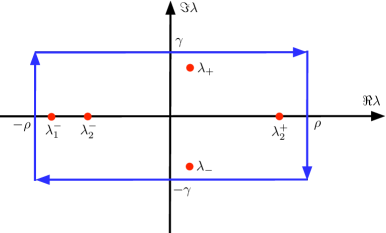
Figure 6: Schematic figure showing a region that contains all eigenvalues $\lambda_{j}^{\tau}$ (red dots) described in Proposition (1 iii) with blue contour used in the integration (134)

The first integral on the right hand side tends to $(u^{-},v^{-})$with $\rho\rightarrow\infty$. Moreover the last two integrals tend to zero for smooth functions $(g,h)$ with compact support. It is enough to prove the theorem for such functions as they are dense in $L_{\gamma}^{+}(\Pi)\cap L_{\gamma}^{-}(\Pi)$.

The residua in (134) belong to the kernel of $(\mathcal{D}(\partial_{x},\partial_{y})-\omega I)$. Therefore the last sum is linear combination of solutions ${\bf w}_{k}^{\tau}$, with $\tau=\pm$ and $k=1,\dots,N$ and we obtain (65) with certian coefficinets. Now, we want to find expressions for those coefficients.

Let us define a smooth function $\eta_{-}=\eta_{-}(y)$ such that $\eta_{-}(y)=1$ in the neighbourhood of $-\infty$ and $\eta_{-}(y)=0$ in the neighbourhood of $+\infty$. Using the biortogonality conditions for functions ${\bf w}_{j}^{\mp}$ in (40) we get

$$\int_{\Pi}\overline{{\bf w}_{j}^{+}}({\mathcal{D}}-\omega I)(\eta_{-}(u^{+},v^{+})^{T}-\eta_{-}(u^{-},v^{-})^{T})dxdy=-iC_{j}^{+}.$$ (135)

Now note that

$$\eta_{-}(u^{-},v^{-}),(1-\eta_{-})(u^{+},v^{+})\in L_{\gamma}^{+}(\Pi)\cap L_{\gamma}^{-}(\Pi).$$

Applying integration by parts, follows

$$\int_{\Pi}\overline{{\bf w}_{j}^{+}}({\mathcal{D}}-\omega I)((1-\eta_{-})(u^{+},v^{+})^{T})dxdy=0$$

and

$$\int_{\Pi}\overline{{\bf w}_{j}^{+}}({\mathcal{D}}-\omega I)(\eta_{-}(u^{-},v^{-})^{T})dxdy=0$$

so from (135), we get

$$\int_{\Pi}\overline{{\bf w}_{j}^{+}}\cdot(g,h)dxdy=-iC_{j}^{+}.$$

In a similar way we obtain

$$\int_{\Pi}\overline{{\bf w}_{j}^{-}}\cdot(g,h)dxdy=iC_{j}^{-}.$$

This furnishes the assertion. ∎

References

- [1] Agmon, S., Douglis, A., Nirenberg, L.: Estimates near the boundary for solutions of elliptic partial differential equations satisfying general boundary conditions II. Comm. Pure Appl. Math. 17 (2), 35-92 (1964)
- [2] Ando, T., Nakanishi, T.: Impurity Scattering in Carbon Nanotubes - Absence of Back Scattering, J. Phys. Soc. Jpn. 67, 1704-1713 (1998).
- [3] Aslanyan, A., Parnovski, L., Vassiliev, D.: Complex resonances in acoustic waveguides. Q. J. Mech Appl Math. 53 (3), 429-447 (2000)
- [4] Brey, L., Fertig, H.A.: Electronic states of graphene nanoribbons studied with the Dirac equation. Phys. Rev. B 73, 235411 (2006)
- [5] Castro Neto, A.H, Guinea, F., Peres, N. M. R., Novoselov,K. S., Geim, A. K.: The electronic properties of graphene, Rev. Mod. Phys. 81, 109 (2009)
- [6] Cardone, G., Nazarov, S.A., Ruotsalainen, K.: Asymptotics of an eigenvalue in the continuous spectrum, Mat. sbornik 203 (2), 3-32 (2012) (English transl.: Sb. Math. 203 (2), 153-182 (2012).
- [7] Chen, Q., Ma, L., Wang, J.: Making graphene nanoribbons: a theoretical exploration. WIREs Comput. Mol. Sci. 6 (3), 243–254 (2016)
- [8] Evans, D.V., Levitin, M., Vasil’ev, D.: Existence theorems for trapped modes. J. Fluid Mech. 261, 21-31 (1994)
- [9] Holst, A., Vassiliev, D.: Edge resonance in an elastic semi-infinite cylinder. Applicable Anal. 74, 479–495 (2000)
- [10] Katsnelson, M. I., Novoselov, K. S., Geim, A. K.: Chiral tunnelling and the Klein paradox in graphene. Nat. Phys. 2, 620-625 (2006)
- [11] Kozlov, V., Maz’ya, V.: Differential equations with operator coefficients with applications to boundary value problems for partial differential equations. Springer Monographs in Mathematics, Springer-Verlag, Berlin (1999)
- [12] Kozlov, V., Maz’ya, V., Rossmann, J.: Elliptic Boundary Value Problems in Domains with Point Singularities. Mathematical Surveys and Monographs 52. Americal Mathematical Society, Providence, (1997)
- [13] Libisch, F., Rotter, S., Burgdörfer, J.: Disorder scattering in graphene nanoribbons. Phys. Status Solidi B, 248 (11), 2598-2603 (2011)
- [14] Linton C.M., McIver P.: Embedded trapped modes in water waves and acoustics. Wave motion. 45, 16-29 (2007)
- [15] Marconcini, P., Macucci, M.: The k · p method and its application to graphene, carbon nanotubes and graphene nanoribbons: the Dirac equation. La Rivista del Nuovo Cimento 45 (8-9), 489-584 (2011)
- [16] Mandelstam, L.I.: Lectures on Optics, Relativity, and Quantum Mechanics. Vol. 2, AN SSSR, Moscow (1947)
- [17] Nazarov, S.A., Plamenevsky, B.A.: Elliptic problems in domains with piecewise smooth boundaries. Walter de Gruyter, Berlin, New York (1994)
- [18] Nazarov, S.A.: Trapped modes for a cylindrical elastic waveguide with a damping gasket. Zh. Vychisl. Mat. i Mat. Fiz. 48 (5), 863-881 (2008) (English transl.: Comput. Math. and Math. Physics. 48 (5), 863-881(2008))
- [19] Nazarov, S.A.: Trapped waves in a cranked waveguide with hard walls.: Acoustic journal. 57 (6), 746-754 (2011) (English transl.: Acoustical Physics. 57 (6), 764-771 (2011))
- [20] Nazarov, S.A.: Asymptotic expansions of eigenvalues in the continuous spectrum of a regularly perturbated quantum waveguide. Theoretical and Mathematical Physics 167 (2), 239-262 (2011) (English transl.: Theoretical and mathematical physics. 167 (2), 606-627 (2011)
- [21] Nazarov, S.A.: Enforced stability of an eigenvalue in the continuous spectrum of a waveguide with an obstacle. Zh. Vychisl. Mat. i Mat. Fiz. 52 (3), 521-538 (2012) (English transl.: Comput. Math. and Math. Physics. 52 (3), 448-464 (2012)
- [22] Nazarov, S.A.: Enforced stability of a simple eigenvalue in the continuous spectrum of a waveguide. Funct. Anal. Appl. 47 (3), 195-209 (2013)ea
- [23] Poynting, J.H.: On the transfer of energy in the electromagnetic field. Phil. Trans. R. Soc. Lond. 175, 343-361 (1884)
- [24] Roitberg, I., Vassiliev, D., Weidl, T.: Edge resonance in an elastic semi-strip. Quart. J. Mech. Appl. Math. 51 (1), 1–13 (1998)
- [25] Umov, N.A.: Equations of Energy Motion in Bodies [in Russian], Odessa (1874)