Neutrino mixing and $R_{K}$ anomaly in $U(1)_{X}$ models:
a bottom-up approach

Abstract

We identify a class of $U(1)_{X}$ models which can explain the $R_{K}$ anomaly and the neutrino mixing pattern, by using a bottom-up approach. The different $X$-charges of lepton generations account for the lepton universality violation required to explain $R_{K}$. In addition to the three right-handed neutrinos needed for the Type-I seesaw mechanism, these minimal models only introduce an additional doublet Higgs and a singlet scalar. While the former helps in reproducing the quark mixing structure, the latter gives masses to neutrinos and the new gauge boson $Z^{\prime}$. Our bottom-up approach determines the $X$-charges of all particles using theoretical consistency and experimental constraints. We find the parameter space allowed by the constraints from neutral meson mixing, rare $b\to s$ decays and direct collider searches for $Z^{\prime}$. Such a $Z^{\prime}$ may be observable at the ongoing run of the Large Hadron Collider with a few hundred fb^-1 of integrated luminosity.

1 Introduction

We live in an era enriched with many experimental breakthroughs and results. The recent discovery of the 125 GeV Higgs boson at the Large Hadron Collider (LHC) has marked the completion of the Standard Model (SM). However, physics beyond the SM (BSM) is certain to exist, and would be needed to explain observations like neutrino masses and mixings, matter-antimatter asymmetry, and dark matter. Although the direct searches performed by the two LHC-based experiments, viz. ATLAS and CMS, have not yet found any new particle, indirect hints of new physics (NP) may still be hidden in the data.

Recently, the LHCb collaboration has reported some indirect hints of BSM physics in the $b\to s\ell\ell$ flavour observables. Major among these are the measurements of $R_{K}$, defined as the ratio of branching fractions of $B^{+}\to K^{+}\mu^{+}\mu^{-}$ and $B^{+}\to K^{+}e^{+}e^{-}$ in the low dilepton mass-squared bin RKexp :

$$R_{K}\equiv\left.\frac{{\rm BR}(B\to K\mu\mu)}{{\rm BR}(B\to Kee)}\right|_{q^{2}=1-6~{}{\rm GeV}^{2}}\;,$$ (1)

and the angular observable $P_{5}^{\prime}$ DescotesGenon:2012zf in the decays of the $B$ mesons in $B\rightarrow K^{*}\mu\mu$ P51 ; P52 . The BELLE collaboration has also reported an anomaly in $P_{5}^{\prime}$ Wehle:2016yoi which is compatible with the one observed in P51 ; P52 . The branching ratio measurements of $B\to K^{*}\mu\mu$ btok* and $B\to\phi\mu\mu$ btophi also show slight deviations from the SM predictions. While the latter anomalies could be accounted for by form factor uncertainties, the $R_{K}$ measurement should be free from strong interaction effects, since the form factors cancel in the ratio. Therefore, if the $R_{K}$ anomaly is confirmed, it would signal a clear lepton flavour universality violation rk_sm_qcd ; rk_sm_qed .

The anomalies in $R_{K}$ and $P_{5}^{\prime}$ measurements can be addressed by invoking additional NP contributions to some of the Wilson coefficients $C_{i}(\mu)$ appearing in the effective Hamiltonian for $b\to s\ell\ell$. In the SM, the effective Hamiltonian for this process is buchalla

$${\mathcal{H}}_{\rm eff} = -\frac{4G_{F}}{\sqrt{2}}V_{tb}V^{*}_{ts}\times$$ (2)

$$\left(\sum_{i=1,6}C_{i}{\mathcal{O}}_{i}+C_{7\gamma}\mathcal{O}_{7\gamma}+C_{8G}{\mathcal{O}}_{8G}+\sum_{i=9,10}C_{i}\mathcal{O}_{i}+\sum_{i=S,P}C_{i}^{(\prime)}\mathcal{O}_{i}^{(\prime)}\right)\;,$$

where $\mathcal{O}_{i}$’s are the effective operators, and ^′ indicates currents with opposite chirality. The values of $C_{i}(m_{b})$ have been calculated in wilson_mb . At the leading order, the additional NP contributions may contribute to the operators which are already present in the SM:

$$\mathcal{O}_{7\gamma} = \frac{e}{16\pi^{2}}m_{b}\left(\bar{s}\sigma_{\mu\nu}P_{R}b\right)F^{\mu\nu}\;,~{}\mathcal{O}_{9}=\frac{\alpha_{e}}{4\pi}\left[\bar{s}\gamma_{\mu}P_{L}b\right]\left[\bar{\ell}\gamma^{\mu}\ell\right]\;,~{}$$

$$\mathcal{O}_{10} = \frac{\alpha_{e}}{4\pi}\left[\bar{s}\gamma_{\mu}P_{L}b\right]\left[\bar{\ell}\gamma^{\mu}\gamma_{5}\ell\right]\;,$$ (3)

or may enhance the effects of the operators whose contributions are normally suppressed by the lepton mass in the SM:

$$\mathcal{O}_{S}=\frac{\alpha_{e}}{4\pi}\left[\bar{s}P_{R}b\right]\left[\bar{\ell}\ell\right]\;, \mathcal{O}_{P}=\frac{\alpha_{e}}{4\pi}\left[\bar{s}P_{R}b\right]\left[\bar{\ell}\gamma_{5}\ell\right],$$

$$\mathcal{O}_{S}^{\prime}=\frac{\alpha_{e}}{4\pi}\left[\bar{s}P_{L}b\right]\left[\bar{\ell}\ell\right]\;, \mathcal{O}_{P}^{\prime}=\frac{\alpha_{e}}{4\pi}\left[\bar{s}P_{L}b\right]\left[\bar{\ell}\gamma_{5}\ell\right]\;,$$ (4)

or may generate new operators which are absent in SM Hiller:2003js :

$$\mathcal{O}^{\prime}_{7\gamma} = \frac{e}{16\pi^{2}}m_{b}\left(\bar{s}\sigma_{\mu\nu}P_{L}b\right)F^{\mu\nu}\;,~{}\mathcal{O}^{\prime}_{9}=\frac{\alpha_{e}}{4\pi}\left[\bar{s}\gamma_{\mu}P_{R}b\right]\left[\bar{\ell}\gamma^{\mu}\ell\right]\;,$$

$$\mathcal{O}_{10}^{\prime} = \frac{\alpha_{e}}{4\pi}\left[\bar{s}\gamma_{\mu}P_{R}b\right]\left[\bar{\ell}\gamma^{\mu}\gamma_{5}\ell\right]\;.$$ (5)

Simultaneous explanation of the $R_{K}$ and $P_{5}^{\prime}$ anomalies is possible if the NP effects are present in ${\mathcal{O}}_{9},{\mathcal{O}}_{9}^{\prime},{\mathcal{O}}_{10}$ or ${\mathcal{O}}_{10}^{\prime}$ operators rk_eft . The global fits  Descotes-Genon:2013wba ; globalfit1 ; globalfit2 ; globalfit3 ; globalfit4 prefer NP effects in $\mathcal{O}_{9}^{\mu}$, i.e. additional contributions to $C_{9}^{\mu}$. Since the observed value of $R_{K}{\rm(obs)}=0.745^{+0.090}_{-0.074}\pm 0.036$ RKexp is less than the SM prediction, which gives $R_{K}$ to be unity within an accuracy of 1%  rk_sm_qcd ; rk_sm_qed , the new physics contribution must interfere destructively with the SM, i.e. opposite to that of $C_{9}^{\rm SM}(m_{b})=4.2$ wilson_mb . This indicates that the sign of $C_{9}^{\text{NP},\mu}$ is negative. The best-fit value of $C_{9}^{\text{NP},\mu}$ is $\approx-1$  Descotes-Genon:2013wba ; globalfit1 ; globalfit2 ; globalfit3 ; globalfit4 ; rk_eft . In addition $C_{9}^{\text{NP},\mu}=-C_{10}^{\text{NP},\mu}$ also gives a good fit to data  globalfit1 ; globalfit2 ; globalfit3 ; globalfit4 . Motivated by these results, many explanations of the anomaly using $Z^{\prime}$  Gauld:2013qba ; Glashow:2014iga ; Bhattacharya:2014wla ; Crivellin:2015mga ; horizontalpaper ; Crivellin:2015era ; Celis:2015ara ; Sierra:2015fma ; Belanger:2015nma ; Gripaios:2015gra ; Allanach:2015gkd ; Fuyuto:2015gmk ; Chiang:2016qov ; Boucenna:2016wpr ; Boucenna:2016qad ; Celis:2016ayl ; Altmannshofer:2016jzy ; Bhattacharya:2016mcc ; Crivellin:2016ejn ; Becirevic:2016zri ; GarciaGarcia:2016nvr and leptoquark rk_eft ; Biswas:2014gga ; Gripaios:2014tna ; Sahoo:2015wya ; Becirevic:2015asa ; Alonso:2015sja ; Calibbi:2015kma ; Huang:2015vpt ; Pas:2015hca ; Bauer:2015knc ; Fajfer:2015ycq ; Barbieri:2015yvd ; Sahoo:2015pzk ; Dorsner:2016wpm ; Sahoo:2016nvx ; Das:2016vkr ; Chen:2016dip ; Becirevic:2016oho ; Becirevic:2016yqi ; Bhattacharya:2016mcc ; Sahoo:2016pet ; Barbieri:2016las ; Cox:2016epl models have been given in the literature.

Since the flavour anomalies mentioned above mostly involve muons, and there is no clear hint of new physics effects in the electron sector apart from $R_{K}$ measurement, most of the analysis have been performed assuming new physics effects in muons only. However, NP contributions in the electron sector, $C_{9}^{\text{NP},e}$, of the same order as those in the muon sector, are still consistent with all $b\to s$ measurements within 2$\sigma$ globalfit1 ; globalfit2 ; globalfit3 ; globalfit4 . The comparisons among two dimensional global fits also prefer ($C_{9}^{\text{NP},e}$, $C_{9}^{\text{NP},\mu}$) over other combinations like ($C_{9}^{\text{NP},\mu}$, $C_{10}^{\text{NP},\mu}$) and ($C_{9}^{\text{NP},\mu}$, ${C_{9}^{\prime~{}\text{NP},\mu}}$), with the best fit point favouring dominant contributions to $C_{9}^{\text{NP},\mu}$ globalfit4 .

In this work, we build our analysis around the choice where NP contributes via the $\mathcal{O}_{9}$ operator. We allow both $C^{\text{NP},e}_{9}$ and $C^{\text{NP},\mu}_{9}$ to be present. Since these two contributions have to be different, the NP must violate lepton flavour universality. This may be implemented in a minimalistic way through an abelian symmetry $U(1)_{X}$, under which the leptons have different charges. In particular, greater NP contribution to $C_{9}^{\text{NP},\mu}$ than $C_{9}^{\text{NP},e}$ may be achieved by a higher magnitude of the $X$-charge for muons than for electrons. Substantial NP contributions to the flavour anomalies also require tree-level flavour-changing neutral currents (FCNC) in the quark sector. These can be implemented through different $X$-charges for the quark generations as well, which should still allow for quark mixing, and be consistent with the flavour physics data.

A horizontal $U(1)_{X}$ symmetry in the lepton sector would also determine the possible textures in the mass matrix of the right-handed neutrinos. In turn, the mixing pattern of the left-handed neutrinos Capozzi:2016rtj ; Esteban:2016qun will be affected through the Type-I seesaw mechanism. The possible textures of the right-handed neutrino mass matrix and the lepton flavour universality violation required for the flavour anomalies can thus have a common origin. Scenarios like an $L_{\mu}-L_{\tau}$ symmetry with $X$-charges given to the SM quarks horizontalpaper ; Altmannshofer:2016jzy or additional vector-like quarks Crivellin:2015mga ; Fuyuto:2015gmk , have been considered in the literature in this context. Other models with $Z^{\prime}$ also have their own $X$-charge assignments Crivellin:2015era ; Celis:2015ara ; Belanger:2015nma ; Allanach:2015gkd ; Celis:2016ayl , however their connection with the neutrino mass matrix has not been explored. We build our model in the bottom-up approach, where we do not assign the $X$-charges a priori, but look for the $X$-charge assignments that satisfy the data in the quark and lepton sectors. As a guiding principle, we introduce a minimal number of additional particles, and ensure that the model is free of any gauge anomalies. Finally, we identify the horizontal symmetries that are compatible with the observed neutrino mixing pattern, and at the same time are able to generate $C_{9}^{\text{NP},e}$ and $C_{9}^{\text{NP},\mu}$ that explain the flavour anomalies.

The paper is organized as follows. In section 2, we describe the construction of the $U(1)_{X}$ models from a bottom-up approach. In section 3, we explore the allowed ranges of the parameters that are consistent with the experimental constraints like neutral meson mixings, rare $B$ decays, and direct collider searches for $Z^{\prime}$. In section 4, we present the predictions for the CP-violating phases in the lepton sectors for specific horizontal symmetries, and project the reach of the LHC for detecting the corresponding $Z^{\prime}$. In section 5, we summarize our results and present our concluding remarks. Further in appendix A, we present the generation of the $Z^{\prime}$ mass and $Z$–$Z^{\prime}$ mixing. In appendix B, we discuss the constraints on the flavour changing neutral interactions from the scalar sector and in appendix C, we calculate the effects of our model on $b\to s\nu\nu$ transitions.

2 Constructing the $U(1)_{X}$ class of models

We construct a class of models wherein, in addition to the SM fields, we also have three right-handed neutrinos that would be instrumental in giving mass to the left-handed neutrinos through the seesaw mechanism. We extend the SM gauge symmetry group by an additional symmetry, $U(1)_{X}$, which corresponds to an additional gauge boson, $Z^{\prime}$, with mass $M_{Z^{\prime}}$ and gauge coupling $g_{Z^{\prime}}$. To start with, we denote the $X$-charge for a SM field $i$ by $X_{i}$. In this section, we shall determine the values of $X_{i}$’s in a bottom-up approach.

2.1 Preliminary constraints on the $X$-charges

Since we wish to build up the model by introducing NP effects only in the $\mathcal{O}_{9}$ operator, we have to make sure that the NP contribution to all the other operators listed in eqs. (3), (4), and (5) should vanish. We first consider the interactions of $Z^{\prime}$ with charged leptons, $\ell$, in the mass basis:

$$\mathcal{L}^{\ell}_{Z^{\prime}}=g_{Z^{\prime}}\,\overline{\ell_{L}}\,\gamma^{\mu}V^{\dagger}_{\ell_{L}}\,{\mathcal{X}}_{\ell_{L}}\,V_{\ell_{L}}\,\ell_{L}\,Z^{\prime}_{\mu}+g_{Z^{\prime}}\,\overline{\ell_{R}}\,\gamma^{\mu}V^{\dagger}_{\ell_{R}}\,{\mathcal{X}}_{\ell_{R}}\,V_{\ell_{R}}\,\ell_{R}\,Z^{\prime}_{\mu}\;,$$ (6)

where ${\mathcal{X}}_{\ell_{L}}=\text{diag}\left(X_{e_{L}},X_{\mu_{L}},X_{\tau_{L}}\right)$ and ${\mathcal{X}}_{\ell_{R}}=\text{diag}\left(X_{e_{R}},X_{\mu_{R}},X_{\tau_{R}}\right)$, while $V_{\ell_{L}}$ and $V_{\ell_{R}}$ are the rotation matrices diagonalizing the Yukawa matrix for charged leptons. Note that the $SU(2)_{L}$ gauge invariance of the SM ensures ${\mathcal{X}}_{\ell_{L}}={\mathcal{X}}_{{\nu_{\ell}}_{L}}$.

The Lagrangian in eq. (6) may be rewritten as

$$\mathcal{L}^{\ell}_{Z^{\prime}} = \frac{1}{2}\,g_{Z^{\prime}}\,\overline{\ell}\,\gamma^{\mu}\left(V^{\dagger}_{\ell_{L}}{\mathcal{X}}_{\ell_{L}}V_{\ell_{L}}+V^{\dagger}_{\ell_{R}}{\mathcal{X}}_{\ell_{R}}V_{\ell_{R}}\right)\ell\,Z^{\prime}_{\mu}$$ (7)

$$-\frac{1}{2}\,g_{Z^{\prime}}\,\overline{\ell}\,\gamma^{\mu}\gamma_{5}\left(V^{\dagger}_{\ell_{L}}{\mathcal{X}}_{\ell_{L}}V_{\ell_{L}}-V^{\dagger}_{\ell_{R}}{\mathcal{X}}_{\ell_{R}}V_{\ell_{R}}\right)\ell\,Z^{\prime}_{\mu}\;.$$

The second term in eq. (7) would contribute to $\mathcal{O}_{10}$ and $\mathcal{O}_{10}^{\prime}$. Since we do not desire such a contribution, we require

$$V^{\dagger}_{\ell_{L}}{\mathcal{X}}_{\ell_{L}}V_{\ell_{L}}=V^{\dagger}_{\ell_{R}}{\mathcal{X}}_{\ell_{R}}V_{\ell_{R}}\;.$$ (8)

A straight forward solution to the eq. (8) yields $V_{\ell_{L}}=I$ and $V_{\ell_{R}}=I$ and further ${\mathcal{X}}_{\ell_{L}}={\mathcal{X}}_{\ell_{R}}$. In such a case a non-zero Yukawa matrix would need the Higgs field, $\Phi$, to be a singlet under $U(1)_{X}$. Note that with unequal vector-like charge assignments in the lepton sector, the Yukawa matrix will naturally be diagonal. This therefore is a minimal and consistent solution and we proceed with this in our analysis.

Now we turn to the $Z^{\prime}$ interactions with the $d$-type quarks:

$$\mathcal{L}^{d}_{Z^{\prime}}=g_{Z^{\prime}}\,\overline{d_{L}}\,\gamma^{\mu}V^{\dagger}_{d_{L}}\,{\mathcal{X}}_{d_{L}}\,V_{d_{L}}d_{L}\,Z^{\prime}_{\mu}+g_{Z^{\prime}}\,\overline{d_{R}}\,\gamma^{\mu}V^{\dagger}_{d_{R}}\,{\mathcal{X}}_{d_{R}}\,V_{d_{R}}\,d_{R}\,Z^{\prime}_{\mu}\;,$$ (9)

where ${\mathcal{X}}_{d_{L}}=\text{diag}\left(X_{d_{L}},X_{s_{L}},X_{b_{L}}\right)$, ${\mathcal{X}}_{d_{R}}=\text{diag}\left(X_{d_{R}},X_{s_{R}},X_{b_{R}}\right)$, while $V_{d_{L}}$ and $V_{d_{R}}$ are the rotation matrices which diagonalize the Yukawa matrix for $d$-type quarks. Note that the $SU(2)_{L}$ gauge invariance of the SM ensures ${\mathcal{X}}_{d_{L}}={\mathcal{X}}_{u_{L}}$.

Substantial NP effects require the $X$-charges to be non-universal, thereby generating both $\overline{b_{L}}\gamma^{\mu}s_{L}Z^{\prime}_{\mu}$ and $\overline{b_{R}}\gamma^{\mu}s_{R}Z^{\prime}_{\mu}$ transitions. The presence of $\overline{\ell}\gamma^{\mu}\ell Z^{\prime}_{\mu}$ interactions from eq. (7) will potentially generate both $\mathcal{O}_{9}$ and $\mathcal{O}_{9}^{\prime}$ operators. We would like the NP contributions to $\mathcal{O}_{9}^{\prime}$ operator to be vanishing, which can be ensured if the 2-3 element of $V^{\dagger}_{d_{R}}{\mathcal{X}}_{d_{R}}V_{d_{R}}$ vanishes. Indeed, we would demand a stricter condition to ensure no tree-level FCNC interactions in the right handed $d$-type sector, i.e. $V^{\dagger}_{d_{R}}{\mathcal{X}}_{d_{R}}V_{d_{R}}$ is diagonal. This can be ensured if

$$V_{d_{R}}\approx I\quad\text{or}\quad{\mathcal{X}}_{d_{R}}\propto I\;.$$ (10)

The non-universal charge assignments in the quark sector will also be constrained by the observed neutral meson mixings. In particular, the constraints in the $K$–$\overline{K}$ oscillations are by far the most stringent, and severely constrain the flavour changing $Z^{\prime}$ interaction with the first two generation quarks. This can be accounted if we choose  horizontalpaper ; Allanach:2015gkd

$$X_{d_{L}}=X_{s_{L}}\;,\quad X_{d_{R}}=X_{s_{R}}\;.$$ (11)

Another extremely important constraint stems from the requirement that the theory be free of any gauge anomalies. If the charge assignments are vector-like, i.e.

$${\mathcal{X}}_{u_{L}}={\mathcal{X}}_{d_{L}}={\mathcal{X}}_{u_{R}}={\mathcal{X}}_{d_{R}}\equiv{\mathcal{X}}_{Q}\quad\;,\quad{\mathcal{X}}_{\ell_{L}}={\mathcal{X}}_{{\nu_{\ell}}_{L}}={\mathcal{X}}_{\ell_{R}}={\mathcal{X}}_{{\nu_{\ell}}_{R}}\equiv{\mathcal{X}}_{L}\;,$$ (12)

and are related by the condition

$${\rm Tr}\left[\,3\,{\mathcal{X}}_{Q}+{\mathcal{X}}_{L}\right]=0\;,$$ (13)

the theory is free of all gauge anomalies. The $X$-charge assignments can then be written in a simplified notation as given in table 1. In terms of this notation, the anomaly-free condition is

$$3\,(2x_{1}+x_{3})+y_{e}+y_{\mu}+y_{\tau}=0\;.$$ (14)

Fields	$Q_{1}$	$Q_{2}$	$Q_{3}$	$L_{1}$	$L_{2}$	$L_{3}$	$\Phi$
$U(1)_{X}$	$x_{1}$	$x_{1}$	$x_{3}$	$y_{e}$	$y_{\mu}$	$y_{\tau}$	$0$

Table 1: Vector-like $X$-charge assignments after applying preliminary constraints from the vanishing of NP contributions to $\mathcal{O}_{9}^{\prime}$, $\mathcal{O}_{10}$ and $\mathcal{O}_{10}^{\prime}$ operators, and constraints from $K$–$\overline{K}$ mixing. Here $Q_{i}$ and $L_{i}$ represent the $i^{\rm th}$ generations of quarks and leptons, respectively.

We are now in a position to select the correct alternative in eq. (10). The NP contribution to the ${\mathcal{O}}_{9}$ operator would require $x_{1}$ and $x_{3}$ to be unequal (see section 2.3), i.e. ${\mathcal{X}}_{d_{L}}\neq I$. The vector-like charge assignments then imply ${\mathcal{X}}_{d_{R}}\neq I$, and the only possibility remaining from eq. (10) is $V_{d_{R}}\approx I$. This condition need not be automatically satisfied in our model. In addition, ${\mathcal{X}}_{d_{L}}={\mathcal{X}}_{d_{R}}\neq I$ could create problems in generating the structure of the quark mixing matrix. We shall discuss the way to overcome these issues in section 2.2.1.

2.2 Enlarging the scalar sector

2.2.1 Additional doublet Higgs to generate the CKM matrix

The Yukawa interactions of quarks with the Higgs doublet $\Phi$ are

$$\mathcal{L}_{\rm Yuk}=\overline{Q^{\rm f}_{L}}\,{\mathcal{Y}}^{u}\,\Phi^{c}\,u^{\rm f}_{R}+\overline{Q^{\rm f}_{L}}\,{\mathcal{Y}}^{d}\,\Phi d^{\rm f}_{R}\;.$$ (15)

where the superscript “f” indicates flavour eigenstates. The $X$-charge assignments given in table 1 govern the structure of the Yukawa matrices (${\mathcal{Y}}^{u}$ and ${\mathcal{Y}}^{d}$) as

$${\mathcal{Y}}^{u}=\begin{pmatrix}\times&\times&0\\ \times&\times&0\\ 0&0&\times\end{pmatrix},\quad{\mathcal{Y}}^{d}=\begin{pmatrix}\times&\times&0\\ \times&\times&0\\ 0&0&\times\end{pmatrix}\;,$$ (16)

where $\times$ denote nonzero values. Quarks masses are obtained by diagonalizing the above ${\mathcal{Y}}^{u}$ and ${\mathcal{Y}}^{d}$ matrices using the bi-unitary transformations $V_{u_{L}}^{\dagger}{\mathcal{Y}}^{u}V_{u_{R}}$ and $V_{d_{L}}^{\dagger}{\mathcal{Y}}^{d}V_{d_{R}}$, respectively. Clearly, the rotations would be only in 1-2 sector. Therefore the quark mixing matrix, i.e. $V_{\text{CKM}}=V_{u_{L}}^{\dagger}V_{d_{L}}$ also would have non-trivial rotations only in the $1$-$2$ sector, however this cannot be a complete picture as we know that all the elements of $V_{\rm CKM}$ are non-zero.

The correct form of $V_{\text{CKM}}$ can be obtained if mixings between 1-3 and 2-3 generations are generated. This can be achieved by enlarging the scalar sector of SM through an addition of one more SM-like doublet, $\Phi_{1}$, with $X$-charge equal to $\pm d\,$ where $d=(x_{1}-x_{{3}})$. We choose $X_{\Phi_{1}}=+d$, similar to that in horizontalpaper .

We first show how the 1-3 and 2-3 mixings are generated with the addition of this new Higgs doublet. The generic representations for these doublets $\Phi_{1}$ and $\Phi_{2}\equiv\Phi$ are

$$\Phi_{1} = \begin{pmatrix}\phi_{1}^{+}\\ \frac{1}{\sqrt{2}}[\text{Re}(\phi_{1})+i\text{Im}(\phi_{1})+v_{1}]\end{pmatrix},\quad\Phi_{2}=\begin{pmatrix}\phi_{2}^{+}\\ \frac{1}{\sqrt{2}}[\text{Re}(\phi_{2})+i\text{Im}(\phi_{2})+v_{2}]\end{pmatrix},$$

where $v_{1}$ and $v_{2}$ are vacuum expectation values of the two doublets. There are related by $v_{1}=v\cos\beta$ and $v_{2}=v\sin\beta$, where $v$ is the electroweak vacuum expectation value. With this addition the Lagrangian in eq. (15) gets modified to

$$\mathcal{L}_{\rm Yuk}=\overline{Q^{\rm f}_{L}}\,\bigg{(}{\mathcal{Y}}_{1}^{u}\Phi_{1}^{c}+{\mathcal{Y}}^{u}\Phi_{2}^{c}\bigg{)}u^{\rm f}_{R}+\overline{Q^{\rm f}_{L}}\,\bigg{(}{\mathcal{Y}}_{1}^{d}\Phi_{1}+{\mathcal{Y}}^{d}\Phi_{2}\bigg{)}d^{\rm f}_{R}\;,$$ (17)

where

$${\mathcal{Y}}_{1}^{u}=\begin{pmatrix}0&0&0\\ 0&0&0\\ \times&\times&0\\ \end{pmatrix},\quad{\mathcal{Y}}_{1}^{d}=\begin{pmatrix}0&0&\times\\ 0&0&\times\\ 0&0&0\\ \end{pmatrix}\;.$$ (18)

The bi-unitary transformations would now diagonalize the quark mass matrices as

$$M^{\text{diag}}_{u} = \frac{v}{\sqrt{2}}V^{\dagger}_{u_{L}}\left({\mathcal{Y}}^{u}_{1}\cos\beta+{\mathcal{Y}}^{u}\sin\beta\right)V_{u_{R}}\;,$$ (19)

$$M^{\text{diag}}_{d} = \frac{v}{\sqrt{2}}V^{\dagger}_{d_{L}}\left({\mathcal{Y}}^{d}_{1}\cos\beta+{\mathcal{Y}}^{d}\sin\beta\right)V_{d_{R}}\;.$$ (20)

From eqs. (16), (17) and (18), it may be seen that rotations in 1-2, 1-3 as well as 2-3 sector will now be needed to diagonalize the Yukawa matrices. Appropriate choice of parameters can then reproduce the correct form of $V_{\text{CKM}}$. We choose $V_{u_{L}}=I$, so that $V_{d_{L}}=V_{\text{CKM}}$, which ensures that $Z^{\prime}$ does not introduce any new source of CP violation in $B$–$\overline{B}$ mixing.

Having fixed $V_{u_{L}}$ and $V_{d_{L}}$, we now turn to $V_{u_{R}}$ and $V_{d_{R}}$. The solution to eq. (19) yields $[\mathcal{Y}_{1}^{u}]_{ij}=0$, implying the mixing angle between the 2-3 and 1-3 generation for up type quark is zero. The solution does not constrain the rotation angle between the first and the second generation, which we choose to be vanishing for simplicity. Hence, $V_{u_{R}}$ in our model is $I$.

Note that eq. (10) and subsequent discussion near the end of section 2.1 led to the requirement $V_{d_{R}}\approx I$. We shall now see that this requirement is easily satisfied in this framework. With $V_{d_{L}}=V_{\rm CKM}$, eq. (20) may be written in the form

$$V_{\rm CKM}M^{\rm diag}_{d}V_{d_{R}}^{\dagger}=\begin{pmatrix}\times&\times&\times\\ \times&\times&\times\\ 0&0&\times\\ \end{pmatrix}\;.$$ (21)

It may be seen that $V_{d_{R}}$ with small rotation angles, parametrized as

$$V_{d_{R}}\approx\begin{pmatrix}1&&\theta_{d_{R12}}&&\theta_{d_{R13}}e^{-i\,\delta_{d}}\\ -\theta_{d_{R12}}&&1&&\theta_{d_{R23}}\\ -\theta_{d_{R13}}e^{i\,\delta_{d}}&&-\theta_{d_{R23}}&&1\end{pmatrix}\;,$$ (22)

can lead to the above form, with

$$\theta_{d_{R{23}}}\approx A\lambda^{2}m_{s}/m_{b}\;,\quad\theta_{d_{R{13}}}\approx-A\lambda^{3}m_{d}/m_{b}\;,$$ (23)

where $A$ and $\lambda$ are the Wolfenstein parameters and $m_{d}$, $m_{s}$ and $m_{b}$ are the quark masses. Note that similar observation has been made in horizontalpaper . The value of $\theta_{d_{R12}}$ is not constrained, and can be chosen to be vanishing. Thus, the requirement $V_{d_{R}}\approx 1$ is satisfied.

Note that since $V_{d_{R}}$ is only approximately equal to $I$, small NP contributions to $C_{9}^{\prime}$ are present, However as we shall see in section 2.3, these contributions are roughly $(A\lambda^{2}m_{s})/(m_{b}V_{tb}V_{ts}^{*})$ times the NP contributions to $C_{9}$, and hence can be safely neglected.

2.2.2 Singlet scalar for generating neutrino masses and mixing pattern

Our model has three right handed neutrinos, $\nu_{R}$’s. The Dirac and the Majorana mass terms for neutrinos are

$$\mathcal{L}^{\text{mass}}_{\nu}=-\overline{\nu_{L}}m_{D}\nu_{R}-\frac{1}{2}\overline{\nu^{c}_{R}}M_{R}\nu_{R}+h.c.\;,$$ (24)

where the basis chosen for $\nu_{L}$ is such that the charged lepton mass matrix is diagonal. The active neutrinos would then get their masses through the Type-I seesaw mechanism. The net mass matrix being

$$M_{\nu}=-m_{D}\,M_{R}^{-1}\,m_{D}^{T}\;.$$ (25)

Since the neutrinos are charged under $U(1)_{X}$ with charges ($y_{e}$,$y_{\mu}$ and $y_{\tau}$), the $(\alpha,\beta)$ elements of the Dirac mass matrix $m_{D}$ would be nonzero only when $y_{\alpha}=y_{\beta}$, while the $(\alpha,\beta)$ elements of the Majorana mass matrix $M_{R}$ would be nonzero only when $y_{\alpha}+y_{\beta}=0$. Since the $X$-charges of neutrinos are non-universal and vector-like, the former condition implies that $m_{D}$ is diagonal. (It can have off-diagonal elements if two of the $y_{\alpha}$’s are identical. However we can always choose the $\nu_{R}$ basis such that $m_{D}$ is diagonal.) The allowed elements of $M_{R}$ are also severely restricted, and it will not be possible to have a sufficient number of nonzero elements in $M_{R}$ to be able to generate the neutrino mixing pattern.

To generate the required mixing pattern, we introduce a scalar $S$, which is a SM-singlet, and has an $X$-charge $X_{S}=a$, as a minimal extension of our model. With the addition of this scalar, the Lagrangian in eq. (24) modifies to

$$[\mathcal{L}^{\text{mass},S}_{\nu}]_{\alpha\beta} = [\mathcal{L}^{\text{mass}}_{\nu}]_{\alpha\beta}-\frac{1}{2}[\overline{\nu^{c}_{R}}]_{\alpha}[{\mathcal{Y}}_{R}]_{\alpha\beta}[\nu_{R}]_{\beta}\,S+h.c.\;.$$ (26)

The conditions for $m_{D}$, $M_{R}$ and ${\mathcal{Y}}_{R}$ elements to be non zero are

$${[m_{D}]}_{\alpha\beta} \neq 0\quad\text{if}\quad y_{\alpha}-y_{\beta}=0\;,$$ (27)

$${[M_{R}]}_{\alpha\beta} \neq 0\quad\text{if}\quad y_{\alpha}+y_{\beta}=0\;,$$

$${[{\mathcal{Y}}_{R}]}_{\alpha\beta} \neq 0\quad\text{if}\quad y_{\alpha}+y_{\beta}=\pm a\;.$$ (28)

When $S$ gets a vacuum expectation value $v_{S}$, it contributes to the Majorana mass term for right handed neutrinos which now becomes

$${[M^{S}_{R}]}_{\alpha\beta}={[M_{R}]}_{\alpha\beta}+\frac{v_{S}}{\sqrt{2}}[y_{R}]_{\alpha\beta}\;.$$ (29)

Thus an element of ${[M^{S}_{R}]}_{\alpha\beta}$ will be non-zero if,

$$y_{\alpha}+y_{\beta}=0,\pm a\;.$$ (30)

The textures in the neutrino mass matrix, i.e. the number and location of vanishing elements therein, hold clues to the internal flavour symmetries. Only some specific textures of $M_{R}$ are allowed. While no three-zero textures are consistent with data, specific two-zero textures are allowed Lavoura:2004tu ; 2minors ; textures ; Heeck:2013bla . In addition, most one-zero textures 1minors , and naturally, all no-zero textures, are also permitted. Among the allowed textures, we identify those that can be generated by a $U(1)_{X}$ symmetry with a singlet scalar, i.e. those for which values of $y_{\alpha}$ and $a$ satisfying eq. (30) may be found. These combinations are listed in table 2, and categorized according to the ratio $y_{e}/y_{\mu}$. Note that by the leptonic symmetry combination $p_{e}L_{e}+p_{\mu}L_{\mu}+p_{\tau}L_{\tau}$, we refer to all $U(1)_{X}$ charge combinations, where $p_{e}/y_{e}=p_{\mu}/y_{\mu}=p_{\tau}/y_{\tau}$ (for non zero values $y_{\alpha}$ and $p_{\alpha}$ respectively). It is to be noted that part of the list was already derived in textures ; Heeck:2013bla . Later in section 2.3, we shall examine the consistency of these symmetries with the flavour data.

Note that we would like all the elements of right handed neutrino mass matrix to have similar magnitudes, so it would be natural to have $[M_{R}^{S}]_{\alpha,\beta}\sim\mathcal{O}({v_{S}})$. Our scenario is thus close to a TeV-scale seesaw mechanism Atwood:2007zza .

Category	$y_{e}$/a	$y_{\mu}/a$	$y_{\tau}/a$	Symmetries
A	$0$	$-1$	$0$, $1$	$L_{\mu}$, $L_{\mu}-L_{\tau}$
B	$\frac{1}{2}$	$-\frac{3}{2}$	$\pm\frac{1}{2}$	$L_{e}-3L_{\mu}\pm L_{\tau}$
C	$-\frac{1}{2}$	$-\frac{3}{2}$	$\frac{1}{2}$	$L_{e}+3L_{\mu}-L_{\tau}$
D	$\frac{1}{2}$	$-\frac{1}{2}$	$\pm\frac{1}{2}$, $\pm\frac{3}{2}$	$L_{e}-L_{\mu}\pm L_{\tau}$, $L_{e}-L_{\mu}\pm 3L_{\tau}$
E	$\frac{1}{2}$	$\frac{1}{2}$	$-\frac{1}{2}$, $-\frac{3}{2}$	$L_{e}+L_{\mu}-L_{\tau}$, $L_{e}+L_{\mu}-3L_{\tau}$
F	$\frac{3}{2}$	$-\frac{1}{2}$	$-\frac{1}{2}$	$3L_{e}-L_{\mu}-L_{\tau}$
G	$1$	$0$	$0$	$\,L_{e}$

Table 2: The $X$-charges (in units of $a$) along with the symmetry combinations that are consistent with the neutrino oscillation data Capozzi:2016rtj ; Esteban:2016qun . Note that by the leptonic symmetry combination $p_{e}L_{e}+p_{\mu}L_{\mu}+p_{\tau}L_{\tau}$, we refer to all $U(1)_{X}$ charge combinations, where $p_{e}/y_{e}=p_{\mu}/y_{\mu}=p_{\tau}/y_{\tau}$ (for non zero values $y_{\alpha}$ and $p_{\alpha}$ respectively). In the list we have dropped the cases with lepton flavour universality and the one where $y_{e}=y_{\mu}=0$.

2.2.3 Relating $X$-charges of doublet and singlet scalars

The scalar sector of our model consists of two $SU(2)_{L}$ doublets $\Phi_{1}$ and $\Phi\equiv\Phi_{2}$, and a SM-singlet $S$, with $X$-charges $d$, 0, $a$, respectively. The scalar potential that respects the $SU(2)_{L}\times U(1)_{Y}\times U(1)_{X}$ symmetry is

$$V_{\Phi_{1}\Phi_{2}S} = -m_{11}^{2}\Phi_{1}^{\dagger}\Phi_{1}+\frac{\lambda_{1}}{2}(\Phi_{1}^{\dagger}\Phi_{1})^{2}-m_{22}^{2}\Phi_{2}^{\dagger}\Phi_{2}+\frac{\lambda_{2}}{2}(\Phi_{2}^{\dagger}\Phi_{2})^{2}$$ (31)

$$-m_{S}^{2}S^{\dagger}S+\frac{\lambda_{S}}{2}(S^{\dagger}S)^{2}+\lambda_{3}\,\Phi_{1}^{\dagger}\Phi_{1}\,\Phi_{2}^{\dagger}\Phi_{2}$$

$$+\lambda_{4}\,\Phi_{1}^{\dagger}\Phi_{2}\,\Phi_{2}^{\dagger}\Phi_{1}+\left(\lambda_{1S{{}_{1}}}\Phi_{1}^{\dagger}\Phi_{1}+\lambda_{2{S}}\Phi_{2}^{\dagger}\Phi_{2}\right)S^{\dagger}S\;.$$

The $U(1)_{X}$ symmetry is broken spontaneously by the vacuum expectation values of $\Phi_{1}$ and $S$, and consequently $Z^{\prime}$ obtains a mass (see appendix A). Since the collider bounds indicate $M_{Z^{\prime}}\gtrsim$ TeV, we expect $v_{s}\gtrsim$ TeV (since $v_{1}\lesssim$ electroweak scale).

Therefore, before electroweak symmetry breaking, $U(1)_{X}$ symmetry gets broken spontaneously and the singlet, $S$, gets decoupled. The effective potential for the doublets after $U(1)_{X}$ symmetry breaking

$$V_{\Phi_{1}\Phi_{2}} = -\left(m_{11}^{2}-\frac{\lambda_{1S{{}_{1}}}}{2}v^{2}_{S}\right)\Phi_{1}^{\dagger}\Phi_{1}+\frac{\lambda_{1}}{2}(\Phi_{1}^{\dagger}\Phi_{1})^{2}-\left(m_{22}^{2}-\frac{\lambda_{2{S}}}{2}v^{2}_{S}\right)\Phi_{2}^{\dagger}\Phi_{2}$$ (32)

$$+\frac{\lambda_{2}}{2}(\Phi_{2}^{\dagger}\Phi_{2})^{2}+\lambda_{3}(\Phi_{1}^{\dagger}\Phi_{1})(\Phi_{2}^{\dagger}\Phi_{2})+\lambda_{4}(\Phi_{1}^{\dagger}\Phi_{2})(\Phi_{2}^{\dagger}\Phi_{1}).$$

The potential, $V_{\Phi_{1},\Phi_{2}}$, is invariant under the global transformation $U(1)_{V}\times U(1)_{A}$ such that

$$U(1)_{V}\times U(1)_{A}:\quad\Phi_{1} \rightarrow e^{i(\theta_{V}-\theta_{A})}\Phi_{1},\quad\quad\Phi_{2}\rightarrow e^{i(\theta_{V}+\theta_{A})}\Phi_{2}.$$ (33)

Out of $U(1)_{V}$ and $U(1)_{A}$, only $U(1)_{V}$ can be gauged and identified as $U(1)_{Y}$ since both the doublets should have the same hypercharge. After electro-weak symmetry breaking, along with the gauge symmetries, $U(1)_{A}$ would also be broken spontaneously and would result in a Goldstone boson. This problem would not arise if the potential were not symmetric under $U(1)_{A}$ to begin with, i.e. if it were broken explicitly by a term

$$\Delta V_{\Phi_{1}\Phi_{2}}=-m_{12}^{2}\Phi_{1}^{\dagger}\Phi_{2}\,+h.c.\;.$$ (34)

Note that this can happen naturally in our scenario: the term above can be generated by spontaneously breaking of $U(1)_{X}$ if $X_{S}$ is equal to $X_{\Phi_{1}}$, i.e., if $a=d$, we can have

$$\Delta V_{\Phi_{1}\Phi_{2}S} = -\widetilde{m}_{{12}}\left[S\,\Phi_{1}^{\dagger}\Phi_{2}+S^{\dagger}\,\Phi_{2}^{\dagger}\Phi_{1}\right]\;,$$ (35)

with

$$m_{12}^{2}=\frac{1}{\sqrt{2}}\widetilde{m}_{{12}}v_{S}\;.$$ (36)

Thus the identification $X_{S}=X_{\Phi_{1}}=a$ naturally avoids a massless scalar in our model by modifying the potential as

$$V_{\Phi_{1}\Phi_{2}S}\to V_{\Phi_{1}\Phi_{2}S}+\Delta V_{\Phi_{1}\Phi_{2}S}\;.$$ (37)

2.3 Selection of the desirable symmetry combinations

In this section, we combine the $U(1)_{X}$ symmetries identified in section 2.2.2 with the NP contribution to ${\mathcal{O}}_{9}$ needed to account for the flavour anomalies. The Lagrangian describing the $Z^{\prime}$ interactions with $d$-type quarks and charged leptons is

$$\mathcal{L}_{Z^{\prime}} = g_{Z^{\prime}}\,\overline{d_{L}}\gamma^{\mu}\,V^{\dagger}_{\text{CKM}}\,{\mathcal{X}}_{Q}\,V_{\text{CKM}}d_{L}\,Z^{\prime}_{\mu}+g_{Z^{\prime}}\,\overline{d_{R}}\,\gamma^{\mu}\,V^{\dagger}_{d_{R}}\,{\mathcal{X}}_{Q}\,V_{d_{R}}\,d_{R}\,Z^{\prime}_{\mu}$$ (38)

$$+g_{Z^{\prime}}\,\overline{\ell}\,\gamma^{\mu}\,{\mathcal{X}}_{L}\,\ell\,Z^{\prime}_{\mu}$$

Here ${\mathcal{X}}_{Q}=\text{diag}(x_{1},x_{1},x_{3})$ and ${\mathcal{X}}_{L}=\text{diag}(y_{e},y_{\mu},y_{\tau})$. Using the above Lagrangian, the $Z^{\prime}$ contributions to the effective Hamiltonian for $b\to s\ell\ell$ processes at $M_{Z^{\prime}}$ scale is

$$\mathcal{H_{\text{eff}}^{\text{NP}}}=-\frac{(x_{1}-x_{3})\,y_{\ell}\,g^{2}_{Z^{\prime}}}{M^{2}_{Z^{\prime}}}V_{tb}V_{ts}^{*}\left(\overline{s_{L}}\gamma^{\mu}b_{L}\right)\left(\overline{\ell}\gamma_{\mu}\ell\right)+\frac{(x_{1}-x_{3})\,y_{\ell}\,g^{2}_{Z^{\prime}}}{M^{2}_{Z^{\prime}}}\theta^{2}_{d_{R23}}\left(\overline{s_{R}}\gamma^{\mu}b_{R}\right)\left(\overline{\ell}\gamma_{\mu}\ell\right)\;.$$ (39)

Comparing it with the standard definition of $\mathcal{H_{\text{eff}}}$ as given in eq. (2), we obtain the NP contribution to the Wilson coefficients $C_{9}^{{\rm NP},\ell}$ and $C_{9}^{\prime\,{\rm NP},\ell}$ as

$$C_{9}^{\text{NP},\ell}(M_{Z}{{}^{\prime}})=\frac{\sqrt{2}\pi(x_{1}-x_{3})\,y_{\ell}g^{2}_{Z^{\prime}}}{G_{F}M^{2}_{Z^{\prime}}\alpha_{e}}\;,\quad C_{9}^{\prime\,{\rm NP},\ell}(M_{Z}{{}^{\prime}})=-\frac{\sqrt{2}\pi(x_{1}-x_{3})\,y_{\ell}g^{2}_{Z^{\prime}}\theta^{2}_{d_{R23}}}{G_{F}M^{2}_{Z^{\prime}}\alpha_{e}V_{tb}V_{ts}^{*}}\;,$$ (40)

The smallness of $\theta_{R23}$, as shown in eq (23), makes the NP contribution to ${\mathcal{O}}_{9}^{\prime}$ small in comparison to the corresponding contribution to ${\mathcal{O}}_{9}$:

$$C_{9}^{\prime\ell}(M_{Z}{{}^{\prime}}) = -\frac{\theta^{2}_{D_{R23}}}{V_{tb}V_{ts}^{*}}\,\,C_{9}^{\text{NP},\ell}(M_{Z}{{}^{\prime}})$$ (41)

$$\approx-0.025\,C_{9}^{\text{NP},\ell}(M_{Z}{{}^{\prime}})\;.$$

The flavour anomalies like $R_{K}$ and $P_{5}^{\prime}$ depend crucially on $C_{9}^{\text{NP},e}$ and $C_{9}^{\text{NP},\mu}$, and not on $C_{9}^{\text{NP},\tau}$. A negative value of $C_{9}^{\text{NP},\mu}$ is preferred Descotes-Genon:2013wba ; globalfit1 ; globalfit2 ; globalfit3 ; globalfit4 as a solution to these anomalies which can be easily obtained if, $(x_{1}-x_{3})\,y_{\mu}<0$. The values of $C_{9}^{\text{NP},e}$ and $C_{9}^{\text{NP},\mu}$ are related by

$$C_{9}^{\text{NP},e}/C_{9}^{\text{NP},\mu}=y_{e}/y_{\mu}\;.$$ (42)

This ratio stays the same at all scales between $M_{Z^{\prime}}$ and $m_{b}$, since the $\mathcal{O}_{9}$ operator does not mix with any other operator at one loop in QCD. This ratio is represented in figure 1 by lines corresponding to different symmetries in table 2.

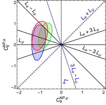
Figure 1: Allowed $1\sigma$ regions in ($C_{9}^{\text{NP},e}$,$C_{9}^{\text{NP},\mu}$) plane using the global fit data: red contour is obtained from globalfit2 , blue from globalfit3 and green from globalfit4 . Lines for various $U(1)_{X}$ symmetries using eq. (42) have also been plotted. We do not show $\tau$ charge explicitly in the plot.

In figure 1, we also show the 1$\sigma$ contours in the $C_{9}^{\text{NP},\mu}$–$C_{9}^{\text{NP},e}$ plane obtained from the global fits globalfit2 ; globalfit3 ; globalfit4 . For further analysis, we select only those combinations (categories A, B, C, D) which pass through the 1$\sigma$ regions of any of these global fit contours. Among these possibilities, $L_{\mu}-L_{\tau}$ has already been considered in the context of $R_{K}$ Crivellin:2015mga ; horizontalpaper ; Fuyuto:2015gmk ; Altmannshofer:2016jzy , where the NP contribution to $C_{9}^{e}$ is absent. We shall explore the phenomenological consequences of these symmetries in section 3.

Category	Symmetry/Charges	$x_{1}/a$	$x_{2}/a$	$x_{3}/a$	$y_{e}/a$	$y_{\mu}/a$	$y_{\tau}/a$
A	$L_{\mu}-L_{\tau}$	$\frac{1}{3}$	$\frac{1}{3}$	$-\frac{2}{3}$	$0$	$-1$	$1$
	$L_{\mu}$	$\frac{4}{9}$	$\frac{4}{9}$	$-\frac{5}{9}$	$0$	$-1$	$0$
B	$L_{e}-3L_{\mu}+L_{\tau}$	$\frac{7}{18}$	$\frac{7}{18}$	$-\frac{11}{18}$	$\frac{1}{2}$	$-\frac{3}{2}$	$\frac{1}{2}$
	$L_{e}-3L_{\mu}-L_{\tau}$	$\frac{1}{2}$	$\frac{1}{2}$	$-\frac{1}{2}$	$\frac{1}{2}$	$-\frac{3}{2}$	$-\frac{1}{2}$
C	$L_{e}+3L_{\mu}-L_{\tau}$	$\frac{1}{2}$	$\frac{1}{2}$	$-\frac{1}{2}$	$-\frac{1}{2}$	$-\frac{3}{2}$	$\frac{1}{2}$
D	$L_{e}-L_{\mu}+3L_{\tau}$	$\frac{1}{6}$	$\frac{1}{6}$	$-\frac{5}{6}$	$\frac{1}{2}$	$-\frac{1}{2}$	$\frac{3}{2}$
	$L_{e}-L_{\mu}-3L_{\tau}$	$\frac{1}{2}$	$\frac{1}{2}$	$-\frac{1}{2}$	$\frac{1}{2}$	$-\frac{1}{2}$	$-\frac{3}{2}$
	$L_{e}-L_{\mu}+L_{\tau}$	$\frac{5}{18}$	$\frac{5}{18}$	$-\frac{13}{18}$	$\frac{1}{2}$	$-\frac{1}{2}$	$\frac{1}{2}$
	$L_{e}-L_{\mu}-L_{\tau}$	$\frac{7}{18}$	$\frac{7}{18}$	$-\frac{11}{18}$	$\frac{1}{2}$	$-\frac{1}{2}$	$-\frac{1}{2}$

Table 3: Charges of the fermion fields in units of $a$. It can be seen that for all the allowed symmetries we have $(x_{1}-x_{3})\,y_{\mu}<0$.

Note that although we refer to the symmetries by their lepton combinations, quarks are also charged under the $U(1)_{X}$. These charges can be easily obtained from the anomaly eq. (14), and have been given in table 3, in terms of the parameter $a$. Further, note that all the $X$-charges are proportional to $a$. As a result, $a$ and $g_{Z^{\prime}}$ always appear in the combination $ag_{Z^{\prime}}$. We therefore absorb $a$ in the definition of $g_{Z^{\prime}}$:

$$g_{Z^{\prime}}\to a\,g_{Z^{\prime}}\;,$$ (43)

and consider $a=1$ without loss of generality for our further analysis. The interactions of $Z^{\prime}$ then can be expressed in terms of two unknown parameters, $g_{Z^{\prime}}$ and $M_{Z^{\prime}}$. In the next section, we shall subject all the symmetry combinations in table 3 to tests from experimental constraints.

3 Experimental Constraints

Our class of models will be constrained from flavour data and direct searches at the colliders. We choose to work in the decoupling regime where the additional scalars are heavy and do not play any significant role in the phenomenology. This is easily possible by suitable choice of the parameters in eq. (37). This framework naturally induces $Z-Z^{\prime}$ mixing at tree level, which can also be minimized by the choice of these parameters (appendix A). The two parameters that are strongly constrained from the data are the mass and gauge coupling of the new vector boson, $Z^{\prime}$. In this section, we explore the constraints on $M_{Z^{\prime}}$ and $g_{Z^{\prime}}$ from neutral meson mixings, rare $B$ decays, and direct $Z^{\prime}$ searches at colliders.

3.1 Constraints from neutral meson mixings and rare $B$ decays

The FCNC couplings of $Z^{\prime}$ to $d_{L}$-type quarks (note that $V_{d_{L}}=V_{\rm CKM}$) will lead to neutral meson mixings as well as $b\to d$ and $b\to s$ transitions at the tree level, and hence may be expected to give significant BSM contributions to these processes.

The effective Hamiltonian in SM Buras_review that leads to $K-\overline{K}$, $B_{d}-\overline{B_{d}}$ and $B_{s}-\overline{B_{s}}$ mixing is

$$\mathcal{H}^{\text{SM}}_{\text{eff}} = \frac{G_{F}^{2}}{16\pi^{2}}M_{W}^{2}C^{\text{SM}}_{K}(\mu)\big{[}\overline{s}\gamma^{\mu}(1-\gamma_{5})d\big{]}\big{[}\overline{s}\gamma_{\mu}(1-\gamma_{5})d\big{]}$$ (44)

$$+ \frac{G_{F}^{2}}{16\pi^{2}}M_{W}^{2}\left(V_{tb}V^{*}_{td}\right)^{2}C^{\text{SM}}_{B_{d}}(\mu)\left[\overline{b}\gamma^{\mu}(1-\gamma_{5})d\right]\left[\overline{b}\gamma_{\mu}(1-\gamma_{5})d\right]$$

$$+ \frac{G_{F}^{2}}{16\pi^{2}}M_{W}^{2}\left(V_{tb}V^{*}_{ts}\right)^{2}C^{\text{SM}}_{B_{s}}(\mu)\left[\overline{b}\gamma^{\mu}(1-\gamma_{5})s\right]\left[\overline{b}\gamma_{\mu}(1-\gamma_{5})s\right]\;,$$

where $C^{\text{SM}}_{P}(\mu)$ are the Wilson coefficients at the scale $\mu$ for $P=K,B_{d},B_{s}$ and the CKM factors for $K$–$\overline{K}$ mixing are absorbed in $C^{\text{SM}}_{K}(\mu)$ itself.

Contributions due the $Z^{\prime}$ exchange will have the same operator form as in the SM since (i) The FCNC contributions to $\overline{d_{Ri}}\gamma^{\mu}d_{Rj}Z^{\prime}_{\mu}$ operator are small as shown in eqs. (23) and (41), and (ii) we are working in the decoupling limit, where the contributions due to the exchanges of scalars $H^{0}$, $A^{0}$ and $H^{+}$ are negligible (see appendix B). As a result, the total effective Hamiltonian can simply be written with the replacement

$$C^{\rm SM}_{P}(\mu)\to C^{\rm tot}_{P}(\mu)=C^{\rm SM}_{P}(\mu)+C^{\rm NP}_{P}(\mu)\;,$$ (45)

with the Wilson coefficients $C^{\rm NP}_{P}$ at the $M_{Z^{\prime}}$ scale given by

$$C^{\text{NP}}_{K}(M_{Z^{\prime}}) = \frac{{2\pi^{2}\,(x_{1}-x_{3})^{2}\,g^{2}_{Z^{\prime}}\left(V_{td}V^{*}_{ts}\right)^{2}}}{M^{2}_{Z^{\prime}}G_{F}^{2}M_{W}^{2}}\;,$$

$$C^{\text{NP}}_{B_{q}}(M_{Z^{\prime}}) = \frac{{2\pi^{2}\,(x_{1}-x_{3})^{2}\,g^{2}_{Z^{\prime}}}}{M^{2}_{Z^{\prime}}G_{F}^{2}M_{W}^{2}}\quad\rm{where,}\,q=d,s\;.$$ (46)

These Wilson coefficients at one loop in QCD run down to the $M_{W}$ scale as Buras_review

$$C^{\text{NP}}_{P}(M_{W})=\left[\frac{\alpha_{s}(m_{t})}{\alpha_{s}(M_{W})}\right]^{\frac{6}{23}}\,\left[\frac{\alpha_{s}(M_{Z^{\prime}})}{\alpha_{s}(m_{t})}\right]^{\frac{2}{7}}C^{\text{NP}}_{P}(M_{Z^{\prime}})\;.$$ (47)

Since the form of operators corresponding to $C^{\text{NP}}_{P}(\mu)$ and $C^{\text{SM}}_{P}(\mu)$ is the same, the ratio $C^{\text{NP}}_{P}(\mu)/C^{\text{SM}}_{P}(\mu)$ stays the same for all scales below $M_{W}$. Since only this ratio is relevant for the constraints from $P$–$\overline{P}$ mixing, we work in terms of $C^{\text{NP}}_{P}(M_{W})/C^{\text{SM}}_{P}(M_{W})$.

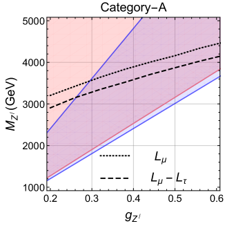
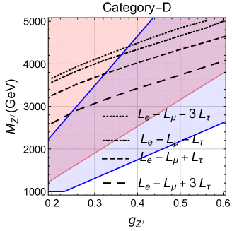
Figure 2: The constraints in the $g_{Z^{\prime}}$ –$M_{Z^{\prime}}$ plane, from neutral meson mixings, rare $B$ decays, and collider searches for $Z^{\prime}$, for the symmetry categories in table 3. The 2$\sigma$ regions allowed by the neutral meson mixings are shaded pink, while the 2$\sigma$ regions allowed by the global fit globalfit4 to $b\to s\ell\ell$ and $b\to s\gamma$ is shaded blue. Purple is the overlap of these two constraints. The dotted and dashed lines correspond to the collider bounds – the regions above them are allowed at 95% C. L.. The net allowed region for a given symmetry is therefore the purple region lying above the dotted / dashed line corresponding to that symmetry.

The constraints from $P$–$\overline{P}$ measurements are generally parametrized in terms of the following quantities UTFit :

$$C_{\epsilon_{K}}\equiv\frac{\text{Im}\left[\left\langle K_{0}|\mathcal{H}^{\text{tot}}_{\text{eff}}|\bar{K_{0}}\right\rangle\right]}{\text{Im}\left[\left\langle K_{0}|\mathcal{H}^{\text{SM}}_{\text{eff}}|\bar{K_{0}}\right\rangle\right]}\;,\quad C_{B_{q}}e^{2i\phi_{B_{q}}}\equiv\frac{\left\langle B_{q}|\mathcal{H}^{\text{tot}}_{\text{eff}}|\bar{B_{q}}\right\rangle}{\left\langle B_{q}|\mathcal{H}^{\text{SM}}_{\text{eff}}|\bar{B_{q}}\right\rangle}\;.$$ (48)

Note that the quantity $C_{\Delta{m_{K}}}\equiv\text{Re}\left[\left\langle K_{0}|\mathcal{H}^{\text{tot}}_{\text{eff}}|\bar{K_{0}}\right\rangle\right]/\text{Re}\left[\left\langle K_{0}|\mathcal{H}^{\text{SM}}_{\text{eff}}|\bar{K_{0}}\right\rangle\right]$ is also a relevant observable, however since it receives large long distance corrections, we do not consider it in our analysis. Since $V_{D_{L}}=V_{\text{CKM}}$, there is no new phase contributions to $B_{q}-\overline{B_{q}}$ mixing and $\phi_{B_{q}}=0$.

We combine the above measurements and show the allowed 2$\sigma$ regions in the $g_{Z^{\prime}}$–$M_{Z^{\prime}}$ plane in figure 2. Note that constraints from neutral meson mixings depends on $g_{Z^{\prime}}$, $M_{Z^{\prime}}$ and $(x_{1}-x_{3})$. Since $(x_{1}-x_{3})=a$, therefore the $P$–$\overline{P}$ constraints are the same in all the categories in table 3 (and hence for all the four panels of figure 2).

Figure 2 also shows the 2$\sigma$ allowed regions that correspond to the constraints from a global fit globalfit4 incorporating the $b\to s\ell\ell$ and $b\to s\gamma$ data. Note that these constraints have already been used in shortlisting the lepton symmetries in table 3, Here we find the allowed regions in the $g_{Z^{\prime}}$–$M_{Z^{\prime}}$ plane using eq. (40). The constraints depend on the $X$-charges of the electron and muon, but are independent of the charge of $\tau$. Therefore we have displayed them in four panels, that correspond to the categories A, B, C, D, respectively.

Our model receives no constraints from $B_{d}\to\mu\mu$ and $B_{s}\to\mu\mu$ since these decays depend on ${\mathcal{O}}_{10}$, and our charge assignments do not introduce any NP contribution to this operator. The NP contribution will affect $b\to s\nu\nu$ decays, however the current upper limits Buras:2014fpa are 4-5 times larger than the SM predictions, whereas in the region that is consistent with the neutral meson mixing and global fits for the rare decays, the enhancement of this decay rate in our model is not more than 10%. See appendix C for further details.

3.2 Direct constraints from collider searches for $Z^{\prime}$

In figure 2 we also show the bounds in the $g_{Z^{\prime}}$–$M_{Z^{\prime}}$ plane from the 95% upper limits on the $\sigma\times{\rm BR}$ for the process $pp\to Z^{\prime}\to\ell\ell$ ATLAS:2016cyf ; CMS:2016abv . The bounds coming from di-jet final state ATLAS:2015nsi ; Sirunyan:2016iap are relatively weaker than those coming from di-leptons, hence we neglect the di-jet bounds in our analysis. The total cross-section $pp\to Z^{\prime}\to\ell\ell$ depends not only on $M_{Z^{\prime}}$ and $g_{Z}^{\prime}$ but also on the $X$-charges of quarks and leptons, therefore the bounds obtained differ for all the nine symmetries in table 3.

Note that the experimental limits in ATLAS:2016cyf ; CMS:2016abv are given in the narrow width approximation, whereas the $Z^{\prime}$ for masses above 2 TeV has broad width for all the symmetry cases which we have considered. The constraints in the broad width case are generally weaker, therefore even lighter $Z^{\prime}$ values than those shown in the figure are allowed.

4 Predictions for neutrino mixing and collider signals

4.1 Neutrino mass ordering and CP-violating Phases

The categories A, B, C and D, in table 3 correspond to different texture-zero symmetries in the right-handed neutrino mass matrix $M_{R}$. Through eq. (29), these predict the light neutrino mass matrix $M_{\nu}$, which can be related to the neutrino masses and mixing parameters via

$$M_{\nu}=-U_{\text{PMNS}}\,M_{\nu}^{\text{diag}}\,U^{T}_{\text{PMNS}}\;,$$ (49)

where $U_{\rm PMNS}$ is the neutrino mixing matrix parametrized by three mixing angles $\theta_{12}$, $\theta_{13}$, $\theta_{23}$, and the Dirac phase $\delta_{cp}$. The diagonal mass matrix $M_{\nu}^{\text{diag}}=(e^{2i\alpha_{1}}m_{1},e^{2i\alpha_{2}}m_{2},m_{3})$ incorporates the Majorana phases $\alpha_{1}$ and $\alpha_{2}$, in addition to the magnitudes of the masses, $m_{1},m_{2}$ and $m_{3}$. Since the symmetries restrict the form of $M_{R}$, they are expected to restrict the possible values of neutrino mixing parameters. While the neutrino mixing angles are reasonable well-measured, the values of unknown parameters like $\alpha_{1},\alpha_{2}$ and $\delta_{\rm CP}$ may be restricted in each of the scenario. In addition, whether the neutrino mass ordering is normal ($m_{2}^{2}<m_{3}^{2}$) or inverted ($m_{2}^{2}>m_{3}^{2}$) is also an open question, and some of the symmetries may have strong preference for one or the other ordering. The symmetries in table 3 that yield two-zero textures for $M_{R}$, viz. $L_{\mu}-L_{\tau}$, $L_{e}-3L_{\mu}-L_{\tau}$, $L_{e}+3L_{\mu}-L_{\tau}$ and $L_{e}-L_{\mu}\pm 3L_{\tau}$ have already been explored in this context and the allowed parameter values determined  Lavoura:2004tu ; 2minors ; Fritzsch:2011qv ; textures ; horizontalpaper .

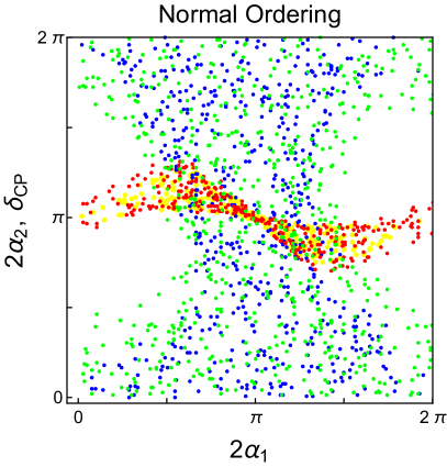
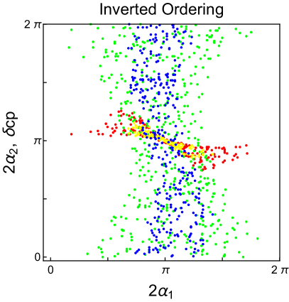
Figure 3: The scatter plots of allowed values of the CP phases $\alpha_{2}$ and $\delta_{\rm CP}$ with the those of $\alpha_{1}$. The left (right) panel shows the results for normal (inverted) mass ordering. The yellow (red) points correspond to $(2\alpha_{1},2\alpha_{2})$ values for $m_{\rm light}=0.05(0.2)$ eV, while the blue (green) points correspond to $(2\alpha_{1},\delta_{\rm CP})$ values for $m_{\rm light}=0.05(0.2)$ eV.

We exemplify the point in the context of the symmetries that yield one-zero texture for $M_{R}$, viz. $L_{\mu}$ and $L_{e}-3L_{\mu}+L_{\tau}$. These two also happen to be the ones that are consistent with all the global fits globalfit1 ; globalfit2 ; globalfit3 ; globalfit4 to the $b\to s\ell\ell$ and $b\to s\gamma$ data to within $1\sigma$. Both of these symmetries lead to $[M_{R}]_{{22}}=0$. Equation (29) then leads to the condition of one vanishing minor in the $M_{\nu}$ mass matrix ma , i.e. $[M_{\nu}]_{11}[M_{\nu}]_{33}-[M_{\nu}]_{13}^{2}=0$. In terms of masses and elements of the $U_{\rm PMNS}$ matrix,

$$\left(U_{13}U_{32}-U_{12}U_{33}\right)^{2}m_{2}m_{3}e^{2i\alpha_{2}} = -\left(U_{12}U_{31}-U_{11}U_{32}\right)^{2}m_{1}m_{2}e^{2i(\alpha_{1}+\alpha_{2})}$$ (50)

$$-\left(U_{13}U_{31}-U_{11}U_{33}\right)^{2}m_{1}m_{3}e^{2i\alpha_{1}}\;,$$

where $U_{ij}$ are elements of the $U_{\text{PMNS}}$ matrix. Requiring the neutrino masses and mixings to satisfy the above relation, we show the allowed values of the CP-violating phases $\alpha_{1},\alpha_{2}$ and $\delta_{\rm CP}$ in figure 3, for two fixed values of the lightest neutrino mass $m_{\rm light}$ (i.e. $m_{1}$ for normal ordering and $m_{3}$ for inverted ordering). We let the other neutrino parameters (mixing angles and mass squared differences) to vary within their $3\sigma$ ranges Capozzi:2016rtj ; Esteban:2016qun . The figure shows that the allowed value of $\alpha_{2}$ with the $L_{\mu}$ or $L_{e}-3L_{\mu}+L_{\tau}$ symmetry is restricted to be rather close to $\pi/2$. For lower $m_{\rm light}$ values, $\alpha_{2}$ is more severely restricted and for inverted ordering, the value of $\alpha_{1}$ also is restricted to be close to $\pi/2$.

Another set of predictions may be obtained by relating the lightest neutrino mass $m_{\rm light}$ to the effective mass measured by the neutrinoless double beta decay experiments Agostini:2013mzu if the neutrinos are Majorana, i.e.

$$\langle m_{ee}\rangle=\left|m_{1}e^{2i\alpha_{1}}\cos^{2}\theta_{12}\cos^{2}\theta_{13}+m_{2}e^{2i\alpha_{2}}\sin^{2}\theta_{12}\cos^{2}\theta_{13}+m_{3}e^{-2i\delta_{\rm CP}}\sin^{2}\theta_{13}\right|\;.$$ (51)

We show the allowed region (with mixing angles and mass squared differences varied within their $3\sigma$ ranges Capozzi:2016rtj ; Esteban:2016qun ) in the $m_{\rm light}$–$\langle m_{ee}\rangle$ plane in figure 4. Bounds from the non-observation of neutrinoless double beta decay Agostini:2013mzu and conservative limits coming from cosmology ($\sum m_{\nu}<0.6$ eV) cosmo have also been shown. The figure shows that the symmetries $L_{\mu}$ or $L_{e}-3L_{\mu}+L_{\tau}$ restrict the allowed values of $m_{\rm light}$ and $\langle m_{ee}\rangle$ significantly in the case of inverted ordering: $m_{\rm light}\gtrsim 0.045$ eV and $\langle m_{ee}\rangle\gtrsim 0.055$ eV. With the cosmological bounds on the sum of neutrino masses becoming stronger, the inverted hierarchy in these scenarios would get strongly disfavoured.

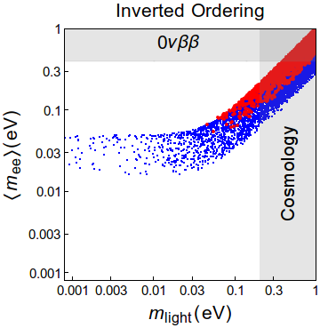
Figure 4: The scatter plots of allowed values of $m_{\rm light}$ and $\langle m_{ee}\rangle$. The red (blue) points correspond to the allowed values with (without) the symmetry ($L_{\mu}$ or $L_{e}-3L_{\mu}+L_{\tau}$). The left (right) panel shows the results for normal (inverted) mass ordering. The regions disallowed by the non-observations of neutrinoless double beta decay ($0\nu\beta\beta$) and cosmological constraints have also been shown.

The symmetries in table 3 that do not lead to a zero-texture in $M_{R}$, i.e. $L_{e}-L_{\mu}\pm L_{\tau}$, will not give any predictions for the neutrino mass ordering or CP-violating phases; model parameters can always be tuned to satisfy the data.

4.2 Prospects of detecting $Z^{\prime}$ at the LHC

In our model apart from $Z^{\prime}$, there are additional scalars and three heavy majorana neutrinos. Note that the parameters in our model have been chosen such that we are in the decoupling limit, i.e. the additional scalars $H,A,H^{\pm},S$ are too heavy to affect any predictions in the model. The three right handed neutrinos in our model have masses of the order of a TeV and hence can be looked at the collider-based experiments. The recent analyses for the detection of the heavy right handed neutrinos can be found in Antusch:2016ejd . We however choose $M_{R}\gtrsim M_{Z^{\prime}}/2$, hence do not consider the phenomenology of the right handed neutrinos.

We shall now explore the possibility of a direct detection of the $Z^{\prime}$ gauge boson in the 13 TeV LHC run. The cleanest probe for this search is $pp\to Z^{\prime}\to\ell\ell$  ATLAS:2016cyf ; CMS:2016abv . In such a search, one looks for a peak in the invariant mass spectrum of the dilepton pair.

As an example, we choose the $L_{e}-3L_{\mu}+L_{\tau}$ symmetry. We use FeynRules Alloul:2013bka to generate the model files and then interface the Madgraph madgraph output of the model with PYTHIA 6.4  Sjostrand:2006za for showering and hadronisation with parton distribution function CTEQ-6 Pumplin:2002vw . The output is then fed into Delphes 3.3 Ovyn:2009tx ; deFavereau:2013fsa which gives the output in the ROOT Antcheva:2009zz format for a semi-realistic detector simulation while using the default ATLAS card. In our detector analysis jets are constructed from particle flow algorithm using the anti-$k_{T}$ jet algorithm with $R=0.5$ and $p_{T}^{\text{min}}=50$ GeV. We retain events only with a pair of isolated opposite-sign muons with highest $p_{T}$ in each event. Care has been taken to reject any isolated electron in the event sample. A rough $p_{T}$ cut on the muons is set at $p_{T}^{\mu}>25$ GeV which roughly matches the ATLAS cuts ATLAS:2016cyf . The dominant SM background for this di-muon channel comes from the Drell-Yann process. Other factors contributing to the SM background are diboson and top quarks in the final state. In the left panel of figure 5 we show the dimuon invariant mass distribution of the SM backgrounds as well as the signal for a fixed benchmark scenario satisfying all the flavour and collider constraints (see figure 2) with $M_{Z^{\prime}}=4$ TeV and $g_{Z^{\prime}}=0.36$. Although the production cross section for such a heavy $Z^{\prime}$ gauge boson is small, close to 1.49 fb, the SM background is also minuscule in that regime. Therefore, the $Z^{\prime}\to\mu\mu$ is a natural probe to look for BSM signals. We note in passing that a $Z^{\prime}$ associated with a hard jet in the final state should increase the signal significance further Khachatryan:2016crw . However, we only select events with opposite sign di-muon pair and a hard jet veto.

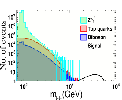
Figure 5: The left panel shows the dimuon invariant mass distribution for the signal originating from $Z^{\prime}$ (with $M_{Z^{\prime}}=4$ TeV and $g_{Z^{\prime}}=0.36$) and the various SM backgrounds at 13 TeV, with $\mathcal{L}=100$ fb^-1. The right panel shows the discovery significance $S/\sqrt{S+B}$ as a function of $M_{Z^{\prime}}$ (with $g_{Z^{\prime}}=0.36$) and integrated luminosity. The $5~{}\sigma$ and $3~{}\sigma$ contours are also shown explicitly.

To further calculate the reach of the LHC for the $Z^{\prime}$ discovery via $Z^{\prime}\to\mu\mu$, we use a signal specific cut on the dimuon invariant mass $m_{\mu\mu}>700$ GeV which renders all the SM backgrounds to be very small whereas the signal hardly gets affected. We keep the coupling $g_{Z^{\prime}}$ fixed at 0.36, and illustrate in the right panel of figure 5, the reach of the LHC in the $M_{Z^{\prime}}$– integrated luminosity ($\mathcal{L}$) plane, in the form of a density plot of the significance $S/\sqrt{S+B}$  dEnterria:2007iyi . (Here $S,~{}B$ are the number of signal and background events after the cut, respectively.) The figure indicates that detecting a $Z^{\prime}$ of mass 4000 GeV at $3~{}\sigma$ ($5~{}\sigma$) significance requires an integrated luminosity close to 400 fb^-1 (1000 fb^-1) in the 13 TeV run of the LHC.

5 Summary and concluding remarks

In this paper, we have looked for a class of models with an additional possible $U(1)_{X}$ symmetry that can explain the flavour anomalies ($R_{K}$ and $P_{5}^{\prime}$) and neutrino mixing pattern. The models are built around the phenomenological choice where NP effects are dominant only in the $\mathcal{O}_{9}$ operator, as indicated by the global fits to the $b\to s$ data. One salient feature of our analysis is that the assignment of $X$-charges of fields is done in a bottom-up approach. I.e., we do not start with a pre-visioned symmetry, but look for symmetry combinations consistent with both the flavour data and neutrino mixing.

In order to generate neutrino masses through the Type-I seesaw mechanism, we add three right-handed neutrinos to the SM field content. This also allows us to assign vector-like $X$-charges to the SM fermions, so that the anomaly cancellation can be easily achieved. This choice also makes NP contributions to ${\mathcal{O}}_{10}$ and ${\mathcal{O}}_{10}^{\prime}$ vanish. While the different $X$-charge assignments to the SM generations introduce the desired element of lepton flavour non-universality at tree level, it also introduces the problem of generating mixings in both quark and lepton sector. This is alleviated by adding an additional doublet Higgs $\Phi_{1}$ that generates the required quark mixing, and a scalar $S$ that generates lepton mixing. The choice of rotation matrices $V_{u_{L}}=V_{u_{R}}=1$, $V_{d_{L}}=V_{\rm CKM}$ and $V_{d_{R}}\approx 1$ also ensures that the NP contribution to ${\mathcal{O}}_{9}^{\prime}$ is negligible. The scalar $S$ also helps in avoiding the possible problem of a Goldstone boson appearing from the breaking of a symmetry in the doublet Higgs sector.

Our model is thus rather parsimonious, with the introduction of only the two additional scalar fields $\Phi_{1}$ and $S$. The symmetry breaking due to the vacuum expectation values of these scalars gives mass to the new gauge boson $Z^{\prime}$, at the same time keeping its mixing with the SM $Z$ boson under control.

With the $X$-charges of quark and lepton generations connected through anomaly cancellation, the $X$-charge assignments may be referred to in terms of the corresponding symmetries in the lepton sector. We identify those leptonic symmetries that would give rise to the required structure in the neutrino mass matrix, at the same time are consistent with the global fits to the $b\to s$ data. We find nine such symmetries, viz. $L_{\mu}-L_{\tau}$, $L_{\mu}$, $L_{e}-3L_{\mu}\pm L_{\tau}$, $L_{e}+3L_{\mu}-L_{\tau}$, $L_{e}-L_{\mu}\pm 3L_{\tau}$, and $L_{e}-L_{\mu}\pm L_{\tau}$. We find the allowed regions in the $g_{Z^{\prime}}$–$M_{Z^{\prime}}$ parameter space that satisfy the bounds from neutral meson mixings, rare $B$ decays, and direct $Z^{\prime}$ collider searches.

The lepton symmetries give rise to specific textures in the right-handed neutrino mass matrix $M_{R}$, and hence, through seesaw, to patterns in the light neutrino mass matrix. The consequent neutrino masses and mixing parameters are hence restricted by these symmetries. In order to exemplify this, we have focussed on the symmetries $L_{\mu}$ and $L_{e}-3L_{\mu}+L_{\tau}$ that give rise to one zero-texture in $M_{R}$, and are also the most favoured symmetries according to all the $b\to s$ global fits. We have analyzed the correlations among the CP-violating phases $\alpha_{1},\alpha_{2},\delta_{\rm CP}$, and also explored the allowed region in the parameter space of the lightest neutrino mass $m_{\rm light}$ and the effective neutrino mass $\langle m_{ee}\rangle$ measured in the neutrinoless double beta decay. For $L_{e}-3L_{\mu}+L_{\tau}$, we also calculate the reach of the LHC for direct detection of $Z^{\prime}$ through the di-muon channel. We find that discovery of $Z^{\prime}$ with the required mass and gauge coupling is possible with a few hundred fb^-1 integrated luminosity at the 13 TeV run.

Note that the parameters in our minimal model have been chosen such that we are in the decoupling limit, i.e. the additional scalars $H,A,H^{\pm},S$, and the three right-handed neutrinos are too heavy to affect any predictions in the model. Our model thus does not try to account for the flavour anomalies indicated in the semileptonic $b\to c$ decays Amhis:2014hma . These anomalies may be addressed in the extensions of this minimal model to include non-decoupling scenarios (for example, where the charged Higgs is light), or additional charged $W^{\prime\pm}$ gauge bosons. While the former scenario needs to satisfy additional constraints from flavour and collider data, the latter will need mechanisms for giving masses to the new gauge bosons.

In this paper we have presented a class of symmetries that are consistent with the current data, and not applied any aesthetic biases among them. As more data come along, some of these symmetries are sure to be further chosen or discarded. We have chosen the symmetries in the bottom-up approach, and have not tried to explore their possible origins. A curious pattern applicable for some of the symmetries ($L_{\mu}$, $L_{e}-3L_{\mu}+L_{\tau}$ and $L_{e}-L_{\mu}+L_{\tau}$) is that the non-universality of $X$-charges is displayed only by the third generation quarks and the second generation leptons. Such patterns may provide further hints in the search for the more fundamental theory governing the mass generation of quarks and leptons.

Appendix A Mass of $Z^{\prime}$ and $Z$-$Z^{\prime}$ mixing

Our model has three scalar fields: two $SU(2)_{L}$ doublets $\Phi_{1}$, $\Phi\equiv\Phi_{2}$, and one singlet $S$. The Lagrangian describing the kinetic terms of the scalar fields is

$$\mathcal{L}^{\text{kin}}_{\text{scalars}} = \Phi_{1}^{\dagger}\left(\overleftarrow{\partial_{\mu}}-i\frac{g_{1}}{2}W_{\mu}.\sigma-i\frac{g_{2}}{2}B_{1\mu}-ig_{Z^{\prime}}X_{\Phi_{1}}B_{2\mu}\right)$$ (52)

$$\left(\overrightarrow{\partial^{\mu}}+i\frac{g_{1}}{2}W^{\mu}.\sigma+i\frac{g_{2}}{2}B_{1}^{\mu}+ig_{Z^{\prime}}X_{\Phi_{1}}B_{2}^{\mu}\right)\Phi_{1}$$

$$+ \Phi_{2}^{\dagger}\left(\overleftarrow{\partial_{\mu}}-i\frac{g_{1}}{2}W_{\mu}.\sigma-i\frac{g_{2}}{2}B_{1\mu}\right)\left(\overrightarrow{\partial^{\mu}}+i\frac{g_{1}}{2}W^{\mu}.\sigma+i\frac{g_{2}}{2}B_{1}^{\mu}\right)\Phi_{2}$$

$$+ \left(\partial_{\mu}-ig_{Z^{\prime}}X_{S}B_{2\mu}\right)S^{\dagger}\left({\partial^{\mu}}+ig_{Z^{\prime}}X_{S}B_{2}^{\mu}\right)S\;.$$

With the $X$-charge assignments of scalars as $X_{\Phi}=0,X_{\Phi_{1}}=X_{S}=a$ (see section 2.2.3), the spontaneous symmetry breaking leads to the following mass term:

$$\mathcal{L}_{{V}}^{\text{mass}}=\frac{1}{2}\begin{pmatrix}W_{3\mu}&B_{1\mu}&B_{2\mu}\end{pmatrix}M^{2}_{V}\begin{pmatrix}W_{3}^{\mu}\\ B^{\mu}_{1}\\ B^{\mu}_{2}\end{pmatrix}\;,$$ (53)

where

$$M^{2}_{V}=\begin{pmatrix}\frac{1}{4}\,g_{1}^{2}v^{2}&&-\frac{1}{4}\,g_{1}\,g_{2}v^{2}&&-\frac{1}{2}\,a\,g_{1}\,g_{Z^{\prime}}v^{2}\cos^{2}{\beta}\\ -\frac{1}{4}\,g_{1}\,g_{2}v^{2}&&\frac{1}{4}\,g_{2}^{2}v^{2}&&\frac{1}{2}\,a\,g_{2}\,g_{Z^{\prime}}v^{2}\cos^{2}{\beta}\\ -\frac{1}{2}\,a\,g_{1}\,g_{Z^{\prime}}v^{2}\cos^{2}{\beta}&&\,\,\frac{1}{2}\,a\,g_{2}\,g_{Z^{\prime}}v^{2}\cos^{2}{\beta}&&\,\,a^{2}\,g_{Z^{\prime}}^{2}\left(v_{S}^{2}+v^{2}\cos^{2}{\beta}\right)\end{pmatrix}\;.$$ (54)

Since $v\sim$ the electroweak scale, and $v_{S}\gtrsim$ TeV, we can approximate the mass eigenstates $\gamma,Z,Z^{\prime}$ in the limit $v_{S}\gg v$ as Langacker:2008yv

$$\gamma = \sin{\theta_{W}}W_{3\mu}+\cos{\theta_{W}}B_{1\mu}\;,$$ (55)

$$Z \approx \cos{\theta_{Z^{\prime}}}\left(\cos{\theta_{W}}W_{3\mu}-\sin{\theta_{W}}B_{1\mu}\right)-\sin{\theta_{Z^{\prime}}}B_{2\mu}\;,$$ (56)

$$Z^{\prime} \approx \sin{\theta_{Z^{\prime}}}\left(\cos{\theta_{W}}W_{3\mu}-\sin{\theta_{W}}B_{1\mu}\right)+\cos{\theta_{Z^{\prime}}}B_{2\mu}\;,$$ (57)

with masses

$$M_{\gamma} = 0\;,$$ (58)

$$M_{Z}^{2} \approx \frac{1}{4}\left(g_{1}^{2}+g_{2}^{2}\right)v^{2}-\Delta\;,$$ (59)

$$M_{Z^{\prime}}^{2} \approx a^{2}g_{Z^{\prime}}^{2}\left(v_{S}^{2}+v^{2}\cos^{2}{\beta}\right)+\Delta\;.$$ (60)

Here $\tan{\theta_{W}}=g_{2}/g_{1}$,

$$\Delta = \frac{1}{4}\frac{a^{2}\left({g_{1}^{2}+g_{2}^{2}}\right)g_{Z^{\prime}}^{2}\,v^{4}\cos^{4}{\beta}}{\left[a^{2}g_{Z^{\prime}}^{2}\left(v_{S}^{2}+v^{2}\cos^{2}{\beta}\right)-\frac{1}{4}\left(g_{1}^{2}+g_{2}^{2}\right)v^{2}\right]}\;,$$ (61)

$$\sin{\theta_{Z^{\prime}}} \simeq -\frac{1}{{2}}\frac{a\sqrt{g_{1}^{2}+g_{2}^{2}}\,g_{Z^{\prime}}\,v^{2}\cos^{2}{\beta}}{\left[a^{2}g_{Z^{\prime}}^{2}\left(v_{S}^{2}+v^{2}\cos^{2}{\beta}\right)-\frac{1}{4}\left(g_{1}^{2}+g_{2}^{2}\right)v^{2}\right]}\;.$$ (62)

Note that since $v\ll v_{S}$, we have $\Delta\sim v^{2}(g_{1}^{2}+g_{2}^{2})(v/v_{S})^{2}\cos^{4}\beta\ll v^{2}$, and therefore

$$M_{Z^{\prime}}\approx ag_{Z^{\prime}}v_{S}$$ (63)

Also, the $Z$–$Z^{\prime}$ mixing angle $\theta_{Z^{\prime}}$ is given by

$$\sin\theta_{Z^{\prime}}\approx\frac{\sqrt{g_{1}^{2}+g_{2}^{2}}v^{2}\cos^{2}\beta}{2ag_{Z^{\prime}}v_{S}^{2}}=\frac{M_{Z}}{M_{Z^{\prime}}}\frac{v}{v_{S}}\cos^{2}\beta\;.$$ (64)

Thus, the $Z$–$Z^{\prime}$ mixing is automatically suppressed: $\theta_{Z^{\prime}}\sim{\mathcal{O}}(10^{-3})$. Therefore, it would not affect our model.

Appendix B Controlling flavour changing neutral currents mediated by scalars

When the singlet $S$ is heavy and effectively decoupled, the scalar doublets $\Phi_{1}$ and $\Phi_{2}$ can be parameterized as branco

$$H_{1}=\cos{\beta}\,\Phi_{1}+\sin{\beta}\,\Phi_{2}\;,\quad H_{2}=-\sin{\beta}\,\Phi_{1}+\cos{\beta}\,\Phi_{2}\;.$$ (65)

where

$$H_{1} = \begin{pmatrix}0\\ \frac{1}{\sqrt{2}}\big{[}h\,\sin(\alpha-\beta)-H\,\cos(\alpha-\beta)+i\,G^{0}+v\big{]}\end{pmatrix}\;,\quad$$

$$H_{2} = \begin{pmatrix}H^{+}\\ \frac{-1}{\sqrt{2}}\big{[}h\,\cos(\alpha-\beta)+H\,\sin(\alpha-\beta)-i\,A\big{]}\end{pmatrix}\;,$$ (66)

such that only the combination $H_{1}$ gets a vacuum expectation value. Here $h$ is the SM-like Higgs with mass equal to 125 GeV, and $H$, $A$ and $H^{\pm}$ are the heavy Higgs, psuedo-scalar Higgs and the charged Higgs, respectively. The Lagrangian in eqn. (17) expressed in terms of $H_{1}$ and $H_{2}$ is

$$\mathcal{L}_{\rm Yuk} = \overline{Q^{\rm f}_{L}}\,\bigg{[}\left({\mathcal{Y}}_{1}^{u}\cos\beta+{\mathcal{Y}}^{u}\sin\beta\right)H_{1}^{c}-\left({\mathcal{Y}}_{1}^{u}\sin\beta-{\mathcal{Y}}^{u}\cos\beta\right)H_{2}^{c}\bigg{]}u^{\rm f}_{R}$$ (67)

$$+\,\,\overline{Q^{\rm f}_{L}}\,\bigg{[}\left({\mathcal{Y}}_{1}^{d}\cos\beta+{\mathcal{Y}}^{d}\sin\beta\right)H_{1}-\left({\mathcal{Y}}_{1}^{d}\sin\beta-{\mathcal{Y}}^{d}\cos\beta\right)H_{2}\bigg{]}d^{\rm f}_{R}\;.$$

This Lagrangian can be expanded to obtain the flavour changing neutral current (FCNC) interactions mediated by the Higgs bosons. Since the up-type quark mass matrix has been chosen to be flavour diagonal (see section 2.2.1), there are no tree-level FCNC’s in the up sector. The tree-level FCNC’s of $d$-type quarks hence can be written as

$$\mathcal{L}^{\text{FCNC}}_{d}=\frac{1}{\sqrt{2}}\overline{d_{L}}V^{\dagger}_{\rm CKM}\left[\bigg{(}{\mathcal{Y}}_{1}^{d}\sin\beta-{\mathcal{Y}}^{d}\cos\beta\bigg{)}\bigg{(}H\sin{\left(\alpha-\beta\right)}+h\cos{\left(\alpha-\beta\right)}-iA\bigg{)}\right]d_{R}\;.$$ (68)

From the above Lagrangian, it can be seen that the FCNC contributions of $H$ and $A$ have opposite signs and hence they tend to cancel if $\alpha-\beta\approx\frac{\pi}{2}$ and $M_{A}\approx M_{H}$. The FCNC contribution of the light Higgs $h$ also vanishes for $\alpha-\beta\approx\frac{\pi}{2}$. Such limits naturally appear in the decoupling scenarios for two-Higgs doublet models, and can be easily incorporated by the suitable choice of parameters in the eq. (37). The scalar spectrum in our model is $M_{h}\ll M_{H},M_{A},M_{H^{\pm}}\ll M_{S}$.

Note that though the charged Higgs $H^{\pm}$ will not contribute to tree-level FCNC, it will have contributions through the penguin and box diagrams. In the decoupling scenario, such contributions would be miniscule and may be ignored.

Appendix C Enhancement or suppression of $b\to s\nu\nu$

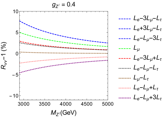
Figure 6: Predictions for $R_{\nu\nu}$ with different symmetries from table 3.

The effective Hamiltonian for $b\to s\nu_{\ell}\nu_{\ell}$ in SM is Buras_review ; Buras:2014fpa

$$\mathcal{H}_{\text{eff}}^{\text{SM}} = -\dfrac{4G_{F}}{\sqrt{2}}\,\frac{\alpha_{e}}{4\pi}\,V_{tb}V_{ts}^{*}\,C^{\text{SM}}_{L}\big{[}\overline{s_{L}}\gamma_{\mu}\,b_{L}\big{]}\,\big{[}\overline{\nu_{\ell}}\gamma_{\mu}(1-\gamma_{5})\nu_{\ell}\big{]}\;,$$ (69)

where $C^{\text{SM}}_{L}=-X_{t}/s_{W}^{2}$, with $X_{t}=1.469\pm 0.017$ Buras:2014fpa . The $Z^{\prime}$ mediation also generates the contribution to the same operator. The combined SM and NP effect is

$$\mathcal{H}_{\text{eff}}^{\text{tot}} = -\dfrac{4G_{F}}{\sqrt{2}}\,\frac{\alpha}{4\pi}\,V_{tb}V_{ts}^{*}\,(C^{\text{SM}}_{L}+C^{\text{NP},\ell}_{L})\big{[}\overline{s_{L}}\gamma_{\mu}\,b_{L}\big{]}\,\big{[}\overline{\nu_{\ell}}\gamma_{\mu}(1-\gamma_{5})\nu_{\ell}\big{]}\;,$$ (70)

with $C^{\text{NP},\ell}_{L}=(x_{1}-x_{3})\pi y_{\ell}g^{2}_{Z^{\prime}}/(\sqrt{2}M^{2}_{Z^{\prime}}G_{F}\alpha_{e})$ The right handed current operator contributions are small (see arguments leading to eq. (41)) and are neglected. NP can enhance the rate of an individual lepton channel $b\to s\nu_{\ell}\nu_{\ell}$ if $(x_{1}-x_{3})y_{\ell}<0$. In experiments, the branching ratios and the decay widths corresponding to $b\to s\nu_{\ell}\nu_{\ell}$ has to summed over all the three generations of neutrinos. We consider the quantity $R_{\nu\nu}$ which gives us a measure of NP effects

$$R_{\nu\nu}=\frac{|C^{\text{SM}}_{L}+C^{\text{NP},e}_{L}|^{2}+|C^{\text{SM}}_{L}+C^{\text{NP},\mu}_{L}|^{2}+|C^{\text{SM}}_{L}+C^{\text{NP},\tau}_{L}|^{2}}{3\,|C^{\text{SM}}_{L}|^{2}}$$ (71)

The enhancement or suppression of the branching ratio crucially depends on the combined effects of $(x_{1}-x_{3})y_{\ell}$ for the three generations.

In figure 6 we show the value of $R_{\nu\nu}$ as a function of $M_{Z^{\prime}}$ for all the symmetries in table 3, where the coupling has been fixed to $g_{Z^{\prime}}=0.4$. It is observed that the net increment is not more than 10% for all symmetries. (Note that for some symmetries, the lower values of masses may not be allowed, as shown in figure 2, in which case the deviation would be further reduced.) The enhancement and suppression is thus too small for the current experiments to be sensitive to – The current bounds on $\text{BR}(B\to K^{(*)}\nu\overline{\nu})$ are 4–5 times higher than the SM prediction Buras:2014fpa , while Belle2 experiment is expected to reach a sensitivity close $30\%$ from SM by 2023 Aushev:2010bq .

References

- (1) R. Aaij et al. [LHCb Collaboration], “Test of lepton universality using decays,” Phys. Rev. Lett. 113 (2014) 151601 [arXiv:1406.6482 [hep-ex]].
- (2) S. Descotes-Genon, J. Matias, M. Ramon and J. Virto, “Implications from clean observables for the binned analysis of at large recoil,” JHEP 1301, 048 (2013) [arXiv:1207.2753 [hep-ph]].
- (3) R. Aaij et al. [LHCb Collaboration], “Measurement of Form-Factor-Independent Observables in the Decay ,” Phys. Rev. Lett. 111, 191801 (2013) [arXiv:1308.1707 [hep-ex]].
- (4) R. Aaij et al. [LHCb Collaboration], “Angular analysis of the decay using 3 fb-1 of integrated luminosity,” JHEP 1602, 104 (2016) [arXiv:1512.04442 [hep-ex]].
- (5) S. Wehle et al. [Belle Collaboration], “Lepton-Flavor-Dependent Angular Analysis of ,” arXiv:1612.05014 [hep-ex].
- (6) R. Aaij et al. [LHCb Collaboration], “Differential branching fractions and isospin asymmetries of decays,” JHEP 1406, 133 (2014) [arXiv:1403.8044 [hep-ex]].
- (7) R. Aaij et al. [LHCb Collaboration], “Differential branching fraction and angular analysis of the decay ,” JHEP 1307, 084 (2013) [arXiv:1305.2168 [hep-ex]].
- (8) C. Bobeth, G. Hiller and G. Piranishvili, “Angular distributions of decays,” JHEP 0712, 040 (2007) [arXiv:0709.4174 [hep-ph]].
- (9) M. Bordone, G. Isidori and A. Pattori, “On the Standard Model predictions for and ,” Eur. Phys. J. C 76, no. 8, 440 (2016) [arXiv:1605.07633 [hep-ph]].
- (10) G. Buchalla, A. J. Buras and M. E. Lautenbacher, “Weak decays beyond leading logarithms,” Rev. Mod. Phys. 68, 1125 (1996) [hep-ph/9512380].
- (11) W. Altmannshofer, P. Ball, A. Bharucha, A. J. Buras, D. M. Straub and M. Wick, “Symmetries and Asymmetries of Decays in the Standard Model and Beyond,” JHEP 0901, 019 (2009) [arXiv:0811.1214 [hep-ph]].
- (12) G. Hiller and F. Kruger, “More model independent analysis of processes,” Phys. Rev. D 69, 074020 (2004) [hep-ph/0310219].
- (13) G. Hiller and M. Schmaltz, “ and future physics beyond the standard model opportunities,” Phys. Rev. D 90, 054014 (2014) [arXiv:1408.1627 [hep-ph]].
- (14) S. Descotes-Genon, J. Matias and J. Virto, “Understanding the Anomaly,” Phys. Rev. D 88, 074002 (2013) [arXiv:1307.5683 [hep-ph]].
- (15) D. Ghosh, M. Nardecchia and S. A. Renner, “Hint of Lepton Flavour Non-Universality in Meson Decays,” JHEP 1412, 131 (2014) [arXiv:1408.4097 [hep-ph]].
- (16) W. Altmannshofer and D. M. Straub, “New physics in transitions after LHC run 1,” Eur. Phys. J. C 75, no. 8, 382 (2015) [arXiv:1411.3161 [hep-ph]].
- (17) S. Descotes-Genon, L. Hofer, J. Matias and J. Virto, “Global analysis of anomalies,” JHEP 1606, 092 (2016) [arXiv:1510.04239 [hep-ph]].
- (18) T. Hurth, F. Mahmoudi and S. Neshatpour, “On the anomalies in the latest LHCb data,” Nucl. Phys. B 909, 737 (2016) [arXiv:1603.00865 [hep-ph]]
- (19) R. Gauld, F. Goertz and U. Haisch, “On minimal explanations of the anomaly,” Phys. Rev. D 89, 015005 (2014) [arXiv:1308.1959 [hep-ph]].
- (20) S. L. Glashow, D. Guadagnoli and K. Lane, “Lepton Flavor Violation in Decays?,” Phys. Rev. Lett. 114, 091801 (2015) [arXiv:1411.0565 [hep-ph]].
- (21) B. Bhattacharya, A. Datta, D. London and S. Shivashankara, “Simultaneous Explanation of the and Puzzles,” Phys. Lett. B 742, 370 (2015) [arXiv:1412.7164 [hep-ph]].
- (22) A. Crivellin, G. D’Ambrosio and J. Heeck, “Explaining , and in a two-Higgs-doublet model with gauged ,” Phys. Rev. Lett. 114, 151801 (2015) [arXiv:1501.00993 [hep-ph]].
- (23) A. Crivellin, G. D’Ambrosio and J. Heeck, “Addressing the LHC flavor anomalies with horizontal gauge symmetries,” Phys. Rev. D 91, no. 7, 075006 (2015) [arXiv:1503.03477 [hep-ph]].
- (24) A. Crivellin, L. Hofer, J. Matias, U. Nierste, S. Pokorski and J. Rosiek, “Lepton-flavour violating decays in generic models,” Phys. Rev. D 92, no. 5, 054013 (2015) [arXiv:1504.07928 [hep-ph]].
- (25) A. Celis, J. Fuentes-Martin, M. Jung and H. Serodio, “Family nonuniversal models with protected flavor-changing interactions,” Phys. Rev. D 92, no. 1, 015007 (2015) [arXiv:1505.03079 [hep-ph]].
- (26) D. Aristizabal Sierra, F. Staub and A. Vicente, “Shedding light on the anomalies with a dark sector,” Phys. Rev. D 92, no. 1, 015001 (2015) [arXiv:1503.06077 [hep-ph]].
- (27) G. Bélanger, C. Delaunay and S. Westhoff, “A Dark Matter Relic From Muon Anomalies,” Phys. Rev. D 92, 055021 (2015) [arXiv:1507.06660 [hep-ph]].
- (28) B. Gripaios, M. Nardecchia and S. A. Renner, “Linear flavour violation and anomalies in B physics,” JHEP 1606, 083 (2016) [arXiv:1509.05020 [hep-ph]].
- (29) B. Allanach, F. S. Queiroz, A. Strumia and S. Sun, “ models for the LHCb and muon anomalies,” Phys. Rev. D 93, no. 5, 055045 (2016) [arXiv:1511.07447 [hep-ph]].
- (30) K. Fuyuto, W. S. Hou and M. Kohda, “ -induced FCNC decays of top, beauty, and strange quarks,” Phys. Rev. D 93, no. 5, 054021 (2016) [arXiv:1512.09026 [hep-ph]].
- (31) C. W. Chiang, X. G. He and G. Valencia, “ model for flavor anomalies,” Phys. Rev. D 93, no. 7, 074003 (2016) [arXiv:1601.07328 [hep-ph]].
- (32) S. M. Boucenna, A. Celis, J. Fuentes-Martin, A. Vicente and J. Virto, “Non-abelian gauge extensions for B-decay anomalies,” Phys. Lett. B 760, 214 (2016) [arXiv:1604.03088 [hep-ph]].
- (33) S. M. Boucenna, A. Celis, J. Fuentes-Martin, A. Vicente and J. Virto, “Phenomenology of an model with lepton-flavour non-universality,” JHEP 1612, 059 (2016) [arXiv:1608.01349 [hep-ph]].
- (34) A. Celis, W. Z. Feng and M. Vollmann, “Dirac Dark Matter and with gauge symmetry,” arXiv:1608.03894 [hep-ph].
- (35) W. Altmannshofer, S. Gori, S. Profumo and F. S. Queiroz, “Explaining dark matter and B decay anomalies with an model,” JHEP 1612, 106 (2016) [arXiv:1609.04026 [hep-ph]].
- (36) A. Crivellin, J. Fuentes-Martin, A. Greljo and G. Isidori, “Lepton Flavor Non-Universality in B decays from Dynamical Yukawas,” Phys. Lett. B 766, 77 (2017) [arXiv:1611.02703 [hep-ph]].
- (37) I. Garcia Garcia, “LHCb anomalies from a natural perspective,” arXiv:1611.03507 [hep-ph].
- (38) D. Bečirević, O. Sumensari and R. Zukanovich Funchal, “Lepton flavor violation in exclusive decays,” Eur. Phys. J. C 76, no. 3, 134 (2016) [arXiv:1602.00881 [hep-ph]].
- (39) B. Bhattacharya, A. Datta, J. P. Guévin, D. London and R. Watanabe, “Simultaneous Explanation of the and Puzzles: a Model Analysis,” arXiv:1609.09078 [hep-ph].
- (40) S. Biswas, D. Chowdhury, S. Han and S. J. Lee, “Explaining the lepton non-universality at the LHCb and CMS within a unified framework,” JHEP 1502, 142 (2015) [arXiv:1409.0882 [hep-ph]].
- (41) B. Gripaios, M. Nardecchia and S. A. Renner, “Composite leptoquarks and anomalies in -meson decays,” JHEP 1505, 006 (2015) [arXiv:1412.1791 [hep-ph]].
- (42) S. Sahoo and R. Mohanta, “Scalar leptoquarks and the rare meson decays,” Phys. Rev. D 91, no. 9, 094019 (2015) [arXiv:1501.05193 [hep-ph]].
- (43) D. Bečirević, S. Fajfer and N. Košnik, “Lepton flavor nonuniversality in processes,” Phys. Rev. D 92, no. 1, 014016 (2015) [arXiv:1503.09024 [hep-ph]].
- (44) R. Alonso, B. Grinstein and J. Martin Camalich, “Lepton universality violation and lepton flavor conservation in -meson decays,” JHEP 1510, 184 (2015) [arXiv:1505.05164 [hep-ph]].
- (45) L. Calibbi, A. Crivellin and T. Ota, “Effective Field Theory Approach to , and with Third Generation Couplings,” Phys. Rev. Lett. 115, 181801 (2015) [arXiv:1506.02661 [hep-ph]].
- (46) W. Huang and Y. L. Tang, “Flavor anomalies at the LHC and the R-parity violating supersymmetric model extended with vectorlike particles,” Phys. Rev. D 92, no. 9, 094015 (2015) [arXiv:1509.08599 [hep-ph]].
- (47) H. Päs and E. Schumacher, “Common origin of and neutrino masses,” Phys. Rev. D 92, no. 11, 114025 (2015) [arXiv:1510.08757 [hep-ph]].
- (48) M. Bauer and M. Neubert, “Minimal Leptoquark Explanation for the R , RK , and Anomalies,” Phys. Rev. Lett. 116, no. 14, 141802 (2016) [arXiv:1511.01900 [hep-ph]].
- (49) S. Fajfer and N. Košnik, “Vector leptoquark resolution of and puzzles,” Phys. Lett. B 755, 270 (2016) [arXiv:1511.06024 [hep-ph]].
- (50) R. Barbieri, G. Isidori, A. Pattori and F. Senia, “Anomalies in -decays and flavour symmetry,” Eur. Phys. J. C 76, no. 2, 67 (2016) [arXiv:1512.01560 [hep-ph]].
- (51) S. Sahoo and R. Mohanta, “Lepton flavor violating B meson decays via a scalar leptoquark,” Phys. Rev. D 93, no. 11, 114001 (2016) [arXiv:1512.04657 [hep-ph]].
- (52) I. Doršner, S. Fajfer, A. Greljo, J. F. Kamenik and N. Košnik, “Physics of leptoquarks in precision experiments and at particle colliders,” Phys. Rept. 641, 1 (2016) [arXiv:1603.04993 [hep-ph]].
- (53) D. Das, C. Hati, G. Kumar and N. Mahajan, “Towards a unified explanation of , and anomalies in a left-right model with leptoquarks,” Phys. Rev. D 94, 055034 (2016) [arXiv:1605.06313 [hep-ph]].
- (54) S. Sahoo and R. Mohanta, “Effects of scalar leptoquark on semileptonic decays,” New J. Phys. 18, no. 9, 093051 (2016) [arXiv:1607.04449 [hep-ph]].
- (55) C. H. Chen, T. Nomura and H. Okada, “, muon , and 750 GeV diphoton excesses in a leptoquark model,” Phys. Rev. D 94, no. 11, 115005 (2016) [arXiv:1607.04857 [hep-ph]].
- (56) D. Bečirević, N. Košnik, O. Sumensari and R. Zukanovich Funchal, “Palatable Leptoquark Scenarios for Lepton Flavor Violation in Exclusive modes,” JHEP 1611, 035 (2016) [arXiv:1608.07583 [hep-ph]].
- (57) D. Bečirević, S. Fajfer, N. Košnik and O. Sumensari, “Leptoquark model to explain the -physics anomalies, and ,” Phys. Rev. D 94, no. 11, 115021 (2016) [arXiv:1608.08501 [hep-ph]].
- (58) S. Sahoo, R. Mohanta and A. K. Giri, “Explaining the and anomalies with vector leptoquarks,” Phys. Rev. D 95, no. 3, 035027 (2017) [arXiv:1609.04367 [hep-ph]].
- (59) R. Barbieri, C. W. Murphy and F. Senia, “B-decay Anomalies in a Composite Leptoquark Model,” Eur. Phys. J. C 77, no. 1, 8 (2017) [arXiv:1611.04930 [hep-ph]].
- (60) P. Cox, A. Kusenko, O. Sumensari and T. T. Yanagida, “SU(5) Unification with TeV-scale Leptoquarks,” arXiv:1612.03923 [hep-ph].
- (61) F. Capozzi, E. Lisi, A. Marrone, D. Montanino and A. Palazzo, “Neutrino masses and mixings: Status of known and unknown parameters,” Nucl. Phys. B 908, 218 (2016) [arXiv:1601.07777 [hep-ph]].
- (62) I. Esteban, M. C. Gonzalez-Garcia, M. Maltoni, I. Martinez-Soler and T. Schwetz, “Updated fit to three neutrino mixing: exploring the accelerator-reactor complementarity,” arXiv:1611.01514 [hep-ph].
- (63) L. Lavoura, “Zeros of the inverted neutrino mass matrix,” Phys. Lett. B 609, 317 (2005) [hep-ph/0411232].
- (64) E. I. Lashin and N. Chamoun, “Zero minors of the neutrino mass matrix,” Phys. Rev. D 78, 073002 (2008) [arXiv:0708.2423 [hep-ph]].
- (65) T. Araki, J. Heeck and J. Kubo, “Vanishing Minors in the Neutrino Mass Matrix from Abelian Gauge Symmetries,” JHEP 1207, 083 (2012) [arXiv:1203.4951 [hep-ph]].
- (66) J. Heeck, “Gauged Flavor Symmetries,” Nucl. Phys. Proc. Suppl. 237-238, 336 (2013).
- (67) E. I. Lashin and N. Chamoun, “One vanishing minor in the neutrino mass matrix,” Phys. Rev. D 80, 093004 (2009) [arXiv:0909.2669 [hep-ph]].
- (68) D. Atwood, S. Bar-Shalom and A. Soni, Phys. Rev. D 76, 033004 (2007) [hep-ph/0701005].
- (69) A. J. Buras, “Weak Hamiltonian, CP violation and rare decays,” hep-ph/9806471.
- (70) UTFIT collaboration, summer 2016 results, http://www.utfit.org
- (71) A. J. Buras, J. Girrbach-Noe, C. Niehoff and D. M. Straub, “ decays in the Standard Model and beyond,” JHEP 1502, 184 (2015) [arXiv:1409.4557 [hep-ph]].
- (72) The ATLAS collaboration [ATLAS Collaboration], “Search for new high-mass resonances in the dilepton final state using proton-proton collisions at = 13 TeV with the ATLAS detector,” ATLAS-CONF-2016-045.
- (73) CMS Collaboration [CMS Collaboration], “Search for a high-mass resonance decaying into a dilepton final state in 13 fb-1 of pp collisions at ,” CMS-PAS-EXO-16-031.
- (74) G. Aad et al. [ATLAS Collaboration], “Search for new phenomena in dijet mass and angular distributions from collisions at 13 TeV with the ATLAS detector,” Phys. Lett. B 754, 302 (2016) [arXiv:1512.01530 [hep-ex]].
- (75) A. M. Sirunyan et al. [CMS Collaboration], “Search for dijet resonances in proton-proton collisions at 13 TeV and constraints on dark matter and other models,” [arXiv:1611.03568 [hep-ex]].
- (76) H. Fritzsch, Z. z. Xing and S. Zhou, “Two-zero Textures of the Majorana Neutrino Mass Matrix and Current Experimental Tests,” JHEP 1109, 083 (2011) [arXiv:1108.4534 [hep-ph]].
- (77) E. Ma, “Connection between the neutrino seesaw mechanism and properties of the Majorana neutrino mass matrix,” Phys. Rev. D 71, 111301 (2005) [hep-ph/0501056].
- (78) M. Agostini et al. [GERDA Collaboration], “Results on Neutrinoless Double- Decay of 76Ge from Phase I of the GERDA Experiment,” Phys. Rev. Lett. 111, no. 12, 122503 (2013) [arXiv:1307.4720 [nucl-ex]].
- (79) Particle Data Group webpage, http://pdg.lbl.gov/2016/listings/rpp2016-list-neutrino-prop.pdf
- (80) S. Antusch, E. Cazzato and O. Fischer, arXiv:1612.02728 [hep-ph].
- (81) A. Alloul, N. D. Christensen, C. Degrande, C. Duhr and B. Fuks, “FeynRules 2.0 - A complete toolbox for tree-level phenomenology,” Comput. Phys. Commun. 185, 2250 (2014) [arXiv:1310.1921 [hep-ph]].
- (82) J. Alwall et al., “The automated computation of tree-level and next-to-leading order differential cross sections, and their matching to parton shower simulations,” JHEP 1407, 079 (2014) [arXiv:1405.0301 [hep-ph]].
- (83) T. Sjostrand, S. Mrenna and P. Z. Skands, “PYTHIA 6.4 Physics and Manual,” JHEP 0605, 026 (2006) [hep-ph/0603175].
- (84) J. Pumplin, D. R. Stump, J. Huston, H. L. Lai, P. M. Nadolsky and W. K. Tung, “New generation of parton distributions with uncertainties from global QCD analysis,” JHEP 0207, 012 (2002) [hep-ph/0201195].
- (85) S. Ovyn, X. Rouby and V. Lemaitre, “DELPHES, a framework for fast simulation of a generic collider experiment,” arXiv:0903.2225 [hep-ph].
- (86) J. de Favereau et al. [DELPHES 3 Collaboration], “DELPHES 3, A modular framework for fast simulation of a generic collider experiment,” JHEP 1402, 057 (2014) [arXiv:1307.6346 [hep-ex]].
- (87) I. Antcheva et al., “ROOT: A C++ framework for petabyte data storage, statistical analysis and visualization,” Comput. Phys. Commun. 180, 2499 (2009) [arXiv:1508.07749 [physics.data-an]].
- (88) V. Khachatryan et al. [CMS Collaboration], “Measurements of the differential production cross sections for a Z boson in association with jets in pp collisions at = 8 TeV,” [arXiv:1611.03844 [hep-ex]].
- (89) D. G. d’Enterria et al. [CMS Collaboration], “CMS physics technical design report: Addendum on high density QCD with heavy ions,” J. Phys. G 34, 2307 (2007).
- (90) Y. Amhis et al. [Heavy Flavor Averaging Group (HFAG)], “Averages of -hadron, -hadron, and -lepton properties as of summer 2014,” arXiv:1412.7515 [hep-ex].
- (91) P. Langacker, “The Physics of Heavy Gauge Bosons,” Rev. Mod. Phys. 81, 1199 (2009) [arXiv:0801.1345 [hep-ph]].
- (92) G. C. Branco, P. M. Ferreira, L. Lavoura, M. N. Rebelo, M. Sher and J. P. Silva, “Theory and phenomenology of two-Higgs-doublet models,” Phys. Rept. 516, 1 (2012) [arXiv:1106.0034 [hep-ph]].
- (93) T. Aushev et al., “Physics at Super B Factory,” arXiv:1002.5012 [hep-ex].