Muon Ionization Cooling Experiment

RAL-P-2017-002

 

Design and expected performance of the MICE demonstration of ionization cooling
The MICE collaboration

Muon beams of low emittance provide the basis for the intense, well-characterised neutrino beams necessary to elucidate the physics of flavour at a neutrino factory and to provide lepton-antilepton collisions at energies of up to several TeV at a muon collider. The international Muon Ionization Cooling Experiment (MICE) aims to demonstrate ionization cooling, the technique by which it is proposed to reduce the phase-space volume occupied by the muon beam at such facilities. In an ionization-cooling channel, the muon beam passes through a material in which it loses energy. The energy lost is then replaced using RF cavities. The combined effect of energy loss and re-acceleration is to reduce the transverse emittance of the beam (transverse cooling). A major revision of the scope of the project was carried out over the summer of 2014. The revised experiment can deliver a demonstration of ionization cooling. The design of the cooling demonstration experiment will be described together with its predicted cooling performance.

1 Introduction

Stored muon beams have been proposed as the source of neutrinos at a neutrino factory [1, 2] and as the means to deliver multi-TeV lepton-antilepton collisions at a muon collider [3, 4]. In such facilities the muon beam is produced from the decay of pions generated by a high-power proton beam striking a target. The tertiary muon beam occupies a large volume in phase space. To optimise the muon yield while maintaining a suitably small aperture in the muon-acceleration system requires that the muon beam be “cooled” (i.e., its phase-space volume reduced) prior to acceleration. A muon is short-lived, decaying with a lifetime of 2.2 $\mu$s in its rest frame. Therefore, beam manipulation at low energy ($\mbox{\raisebox{-1.72218pt}{$\;\stackrel{{\scriptstyle<}}{{\scriptstyle\sim}}\;$}}1$ GeV) must be carried out rapidly. Four cooling techniques are in use at particle accelerators: synchrotron-radiation cooling [5]; laser cooling [6, 7, 8]; stochastic cooling [9]; and electron cooling [10]. Synchrotron-radiation cooling is observed only in electron or positron beams, owing to the relatively low mass of the electron. Laser cooling is limited to certain ions and atomic beams. Stochastic cooling times are dependent on the bandwidth of the stochastic-cooling system relative to the frequency spread of the particle beam. The electron-cooling time is limited by the available electron density and the electron-beam energy and emittance. Typical cooling times are between seconds and hours, long compared with the muon lifetime. Ionization cooling proceeds by passing a muon beam through a material, the absorber, in which it loses energy through ionization, and subsequently restoring the lost energy in accelerating cavities. Transverse and longitudinal momentum are lost in equal proportions in the absorber, while the cavities restore only the momentum component parallel to the beam axis. The net effect of the energy-loss/re-acceleration process is to decrease the ratio of transverse to longitudinal momentum, thereby decreasing the transverse emittance of the beam. In an ionization-cooling channel the cooling time is short enough to allow the muon beam to be cooled efficiently with modest decay losses. Ionization cooling is therefore the technique by which it is proposed to cool muon beams [11, 12, 13]. This technique has never been demonstrated experimentally and such a demonstration is essential for the development of future high-brightness muon accelerators.

The international Muon Ionization Cooling Experiment (MICE) collaboration proposes a two-part process to perform a full demonstration of transverse ionization cooling. First, the “Step IV” configuration [14] will be used to study the material and beam properties that determine the performance of an ionization-cooling lattice. Secondly, a study of transverse-emittance reduction in a cooling cell that includes accelerating cavities will be performed.

The cooling performance of an ionization-cooling cell depends on the emittance and momentum of the initial beam, on the properties of the absorber material and on the transverse betatron function ($\beta_{\perp}$) at the absorber. These factors will be studied using the Step IV configuration. Once this has been done, “sustainable” ionization cooling must be demonstrated. This requires restoring energy lost by the muons as they pass through the absorber using RF cavities. The experimental configuration with which the MICE collaboration originally proposed to study ionization cooling was presented in [15]. This configuration was revised to accelerate the timetable on which a demonstration of ionization cooling could be delivered and to reduce cost. This paper describes the revised lattice proposed by the MICE collaboration for the demonstration of ionization cooling and presents its performance.

2 Cooling in neutrino factories and muon colliders

At production, muons occupy a large volume of phase space. The emittance of the initial muon beam must be reduced before the beam is accelerated. A neutrino factory [16] requires the transverse emittance to be reduced from 15–20 mm to 2–5 mm. A muon collider [17] requires the muon beam to be cooled in all six phase-space dimensions; to achieve the desired luminosity requires an emittance of $\sim 0.025$ mm in the transverse plane and $\sim 70$ mm in the longitudinal direction [18, 19].

Ionization cooling is achieved by passing a muon beam through a material with low atomic number ($Z$), in which it loses energy by ionization, and subsequently accelerating the beam. The rate of change of the normalised transverse emittance, $\varepsilon_{\perp}$, is given approximately by [12, 20, 21]:

$$\frac{\text{d}\varepsilon_{\perp}}{\text{d}z}\backsimeq-\frac{\varepsilon_{\perp}}{\beta^{2}E_{\mu}}\Big{\langle}\frac{\text{d}E}{\text{d}z}\Big{\rangle}+\frac{\beta_{\perp}(13.6\,\text{MeV/}c)^{2}}{2\beta^{3}E_{\mu}m_{\mu}X_{0}}\,;$$ (1)

where $z$ is the longitudinal coordinate, $\beta c$ is the muon velocity, $E_{\mu}$ the energy, $\big{\langle}\frac{\text{d}E}{\text{d}z}\big{\rangle}$ the mean rate of energy loss per unit path-length, $m_{\mu}$ the mass of the muon, $X_{0}$ the radiation length of the absorber and $\beta_{\perp}$ the transverse betatron function at the absorber. The first term of this equation describes “cooling” by ionization energy loss and the second describes “heating” by multiple Coulomb scattering. Equation 1 implies that the equilibrium emittance, for which $\frac{\text{d}\varepsilon_{\perp}}{\text{d}z}=0$, and the asymptotic value of $\frac{\text{d}\varepsilon_{\perp}}{\text{d}z}$ for large emittance are functions of muon-beam energy.

In order to have good performance in an ionization-cooling channel, $\beta_{\perp}$ needs to be minimised and $X_{0}\langle\frac{\text{d}E}{\text{d}z}\rangle$ maximised. The betatron function at the absorber is minimised using a suitable magnetic focusing channel (typically solenoidal) [22, 23] and $X_{0}\langle\frac{\text{d}E}{\text{d}z}\rangle$ is maximised using a low-$Z$ absorber such as liquid hydrogen (LH₂) or lithium hydride (LiH) [24].

3 The Muon Ionization Cooling Experiment

The muons for MICE come from the decay of pions produced at an internal target dipping directly into the circulating proton beam in the ISIS synchrotron at the Rutherford Appleton Laboratory (RAL) [25, 26]. A beam line of 9 quadrupoles, 2 dipoles and a superconducting “decay solenoid” collects and transports the momentum-selected beam into the experiment [27]. The small fraction of pions that remain in the beam may be rejected during analysis using the time-of-flight hodoscopes and Cherenkov counters that are installed in the beam line upstream of the experiment [28]. A diffuser is installed at the upstream end of the experiment to vary the initial emittance of the beam. Ionization cooling depends on momentum through $\beta$, $E_{\mu}$ and $\Big{\langle}\frac{\text{d}E}{\text{d}z}\Big{\rangle}$ as shown in equation 1. It is therefore proposed that the performance of the cell be measured for momenta in the range 140 MeV/c to 240 MeV/$c$ [15].

3.1 The configuration of the ionization-cooling experiment

The configuration proposed for the demonstration of ionization cooling is shown in figure 1. It contains a cooling cell sandwiched between two spectrometer-solenoid modules. The cooling cell is composed of two 201 MHz cavities, one primary (65 mm) and two secondary (32.5 mm) LiH absorbers placed between two superconducting “focus-coil” (FC) modules. Each FC has two separate windings that can be operated either with the same or in opposed polarity.

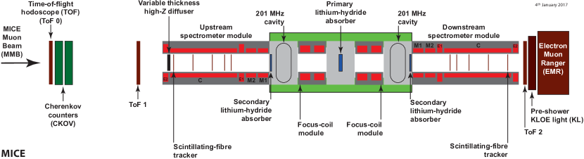
Figure 1: Layout of the lattice configuration for the cooling demonstration. The red rectangles represent the solenoids. The individual coils in the spectrometer solenoids are labelled E1, C, E2, M1 and M2. The ovals represent the RF cavities and the blue rectangles the absorbers. The various detectors (time-of-flight hodoscopes [29, 30], Cerenkov counters [31], scintillating-fibre trackers [32], KLOE Light (KL) calorimeter [27, 33], electron muon ranger [34]) used to characterise the beam are also represented. The green-shaded box indicates the cooling cell.

The emittance is measured upstream and downstream of the cooling cell using scintillating-fibre tracking detectors [32] immersed in the uniform 4 T magnetic field provided by three superconducting coils (E1, C, E2). The trackers are used to reconstruct the trajectories of individual muons at the entrance and exit of the cooling cell. The reconstructed tracks are combined with information from instrumentation upstream and downstream of the spectrometer modules to measure the muon-beam emittance at the upstream and downstream tracker reference planes. The instrumentation upstream and downstream of the spectrometer modules serves to select a pure sample of muons. Time-of-flight hodoscopes are used to determine the time at which the muon crosses the RF cavities. The spectrometer-solenoid magnets also contain two superconducting “matching” coils (M1, M2) that are used to match the optics between the uniform field region and the neighbouring FC.

The secondary LiH absorbers (SAs) are introduced between the cavities and the trackers to minimise the exposure of the trackers to “dark-current” electrons originating from the RF cavities. Experiments at the MuCool Test Area (MTA) at Fermilab [35] have observed that the rate of direct X-ray production from the RF cavities can be managed to ensure it does not damage the trackers [36]. The SAs are introduced to minimise the exposure of the trackers to energetic dark-current electrons that could produce background hits. The SAs are positioned between the trackers and the cavities such that they can be removed to study the empty channel. The SAs increase the net transverse-cooling effect since the betatron functions at these locations are small.

Retractable lead radiation shutters will be installed on rails between the spectrometer solenoids and the RF modules to protect the trackers against dark-current induced radiation during cavity conditioning. The SAs will be mounted on a rail system similar to that which will be used for the lead shutters and will be located between the cavities and the lead shutters. Both mechanisms will be moved using linear piezo-electric motors that operate in vacuum and magnetic field. The design of both the radiation shutter and the movable SA inside the vacuum chamber is shown in figure 2.

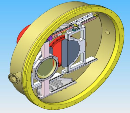
Figure 2: Design of the movable frame for the secondary absorber (front) and the lead radiation shutter (back). The half discs of the lead shutter (grey) can be seen together with the rails (white) inside the vacuum chamber (yellow).

The RF cavities are 201 MHz “pillbox” resonators, 430 mm in length, operating in the TM₀₁₀ mode with large diameter apertures to accommodate the high emittance beam. The apertures are covered by thin (0.38 mm) beryllium windows to define the limits for the accelerating RF fields whilst minimising the scattering of muons. The cavity is excited by two magnetic-loop couplers on opposite sides of the cavity. At the particle rate expected in MICE there is no beam-loading of the RF fields. An effective peak field of 10.3 MV/m is expected for a drive power of 1.6 MW to each cavity. This estimate was used to define the gradient in the simulations described below.

4 Lattice design

4.1 Design parameters

The lattice has been optimised to maximise the reduction in transverse emittance. The optimum is obtained by matching the betatron function to a small value in the central absorber while minimising its maximum values in the FC modules; limiting the size of the betatron function in the FCs helps to reduce the influence of non-linear terms in the magnetic-field expansion. The matching accounts for the change in energy of the muons as they pass through the cooling cell by adjusting currents in the upstream and downstream FCs and in the matching coils in the spectrometer solenoids independently while maintaining the field in the tracking volumes at 4 T. In this configuration, it is also possible to keep the betatron function relatively small at the position of the secondary absorbers whilst maintaining an acceptable beam size at the position of the cavities.

Chromatic aberrations caused by the large momentum spread of the beam ($\sim 5\%$ rms) lead to a chromatic mismatch of the beam in the downstream solenoid unless the phase advance across the cooling cell (i.e., the rate of rotation of the phase-space ellipse) is chosen appropriately. The phase advance of the cell is obtained by integrating the inverse of the beta-function along the beam axis from the reference plane in the upstream spectrometer-solenoid to the reference plane in the downstream spectrometer-solenoid. Such a mismatch reduces the effective transverse-emittance reduction through the chromatic decoherence that results from the superposition of beam evolutions for the different betatron frequencies that result from the range of momenta in the beam. For beams with a large input emittance, spherical aberrations may lead to phase-space filamentation. The chromatic and spherical aberrations were studied by tracking samples of muons through the lattice using the “MICE Analysis User Software” (MAUS, see section 5). The betatron-function and emittance evolution of a 200 MeV/$c$ beam with the initial parameters given in table 1 are shown, for different phase advances, in figures 3 and 4 respectively. The phase advance of $2\pi\times 1.81$ showed the largest transverse-emittance reduction and was therefore chosen. The lattice parameters for this phase advance are presented in table 2.

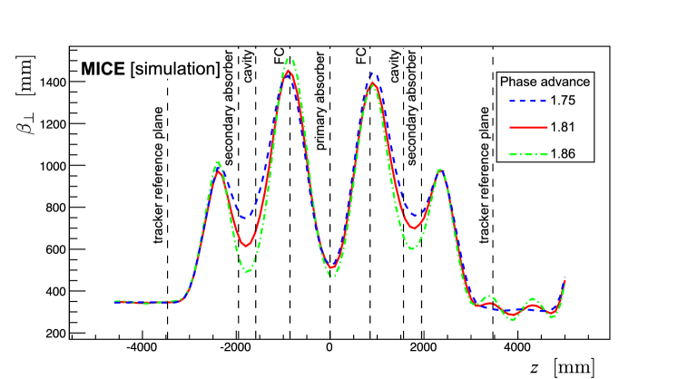
Figure 3: Transverse 4D beta-function versus longitudinal coordinate $z$ in the cooling-demonstration lattice for 200 MeV/$c$ settings with a phase advance of $2\pi\times 1.75$ (dashed blue line), $2\pi\times 1.81$ (solid red line) and $2\pi\times 1.86$ (dot-dashed green line). The vertical dashed lines with labels show the positions of the tracker reference planes and the centres of the absorbers, RF cavities and focus coil modules.

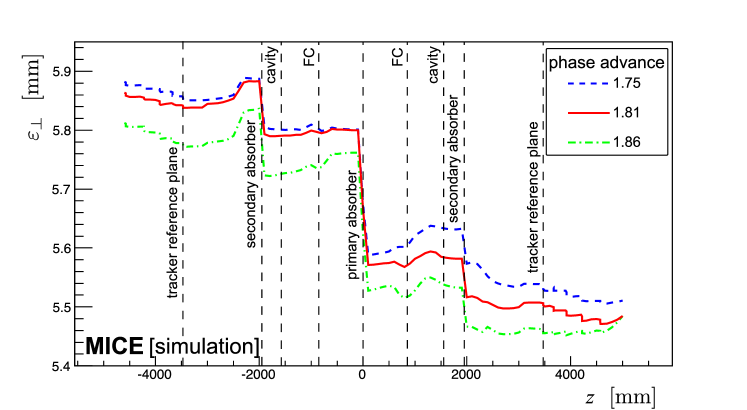
Figure 4: 4D emittance evolution in the cooling-demonstration lattice for 200 MeV/$c$ settings with a phase advance of $2\pi\times 1.75$ (dashed blue line), $2\pi\times 1.81$ (solid red line) and $2\pi\times 1.86$ (dot-dashed green line). The vertical dashed lines with labels show the positions of the tracker reference planes and the centres of the absorbers, RF cavities and focus coil modules.

Table 1: General parameters of the initial beam conditions used in the simulations.

Parameter	Value
Particle	muon $\mu^{+}$
Number of particles	10000
Longitudinal position [mm]	$-4612.1$
Central energy (140 MeV/$c$ settings) [MeV]	175.4
Central energy (200 MeV/$c$ settings) [MeV]	228.0
Central energy (240 MeV/$c$ settings) [MeV]	262.2
Transverse Gaussian distribution:
$\alpha_{\perp}$	0
$\beta_{\perp}$ (140 MeV/$c$ settings) [mm]	233.5
$\varepsilon_{\perp}$ (140 MeV/$c$ settings) [mm]	4.2
$\beta_{\perp}$ (200 MeV/$c$ settings) [mm]	339.0
$\varepsilon_{\perp}$ (200 MeV/$c$ settings) [mm]	6.0
$\beta_{\perp}$ (240 MeV/$c$ settings) [mm]	400.3
$\varepsilon_{\perp}$ (240 MeV/$c$ settings) [mm]	7.2
Longitudinal Gaussian distribution:
Longitudinal emittance [mm]	20
Longitudinal $\beta$ [ns]	11
Longitudinal $\alpha$	$-0.7$
rms momentum spread (140 MeV/$c$ settings)	4.8%
rms time spread (140 MeV/$c$ settings) [ns]	0.40
rms momentum spread (200 MeV/$c$ settings)	4.0%
rms time spread (200 MeV/$c$ settings) [ns]	0.34
rms momentum spread (240 MeV/$c$ settings)	3.6%
rms time spread (240 MeV/$c$ settings) [ns]	0.31

Table 2: Parameters of the cooling-demonstration lattice. $L_{\text{SS}\rightarrow\text{FC}}$ is the distance between the centre of the spectrometer solenoid and the centre of the neighbouring FC, $L_{\text{FC}\rightarrow\text{FC}}$ the distance between the centres of the FCs, and $L_{\text{RF module}\rightarrow\text{FC}}$ the distance between the RF module and the neighbouring FC.

Parameter	Value
Length $L_{\text{SS}\rightarrow\text{FC}}$ [mm]	2607.5
Length $L_{\text{FC}\rightarrow\text{FC}}$ [mm]	1678.8
Length $L_{\text{RF module}\rightarrow\text{FC}}$ [mm]	784.0
RF Gradient [MV/m]	10.3
Number of RF cavities	2
Number of primary absorbers	1
Number of secondary absorbers	2

The currents that produce the optimum magnetic lattice were obtained using the procedure described above for three momentum settings: 140 MeV/$c$, 200 MeV/$c$ and 240 MeV/$c$. The magnetic field on axis for each of these settings is shown in figure 5. The fields in the downstream FC and spectrometer are opposite to those in the upstream FC and spectrometer, the field changing sign at the primary absorber. Such a field flip is required in an ionization cooling channel to reduce the build-up of canonical angular momentum [37]. The currents required to produce the magnetic fields shown in figure 5 are listed in table 3. All currents are within the proven limits of operation for the individual coil windings. The magnetic forces acting on the coils have been analysed and were found to be acceptable. Configurations in which there is no field flip can also be considered.

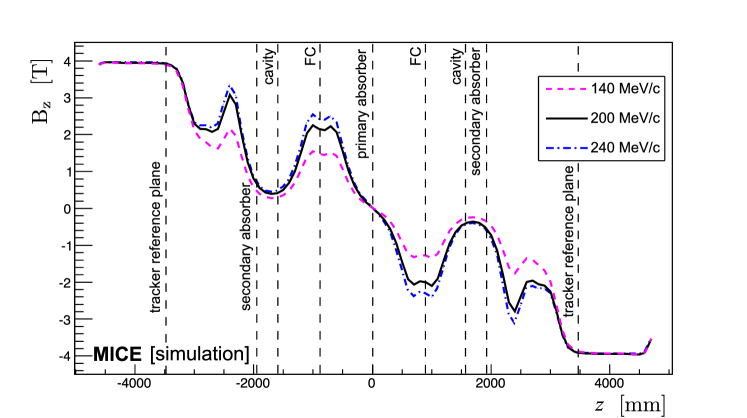
Figure 5: Magnetic field $B_{z}$ on-axis versus the longitudinal coordinate $z$ for the cooling-demonstration lattice design for 200 MeV/$c$ (solid black line), 140 MeV/$c$ (dashed purple line) and 240 MeV/$c$ (dot-dashed blue line) settings. The vertical dashed lines with labels show the positions of the tracker reference planes and the centres of the absorbers, RF cavities and focus coil modules.

Table 3: Coil currents used for 140 MeV/$c$, 200 MeV/$c$ and 240 MeV/$c$ lattice settings.

Coil	140 MeV/$c$ Lattice [A]	200 MeV/$c$ Lattice [A]	240 MeV/$c$ Lattice [A]
Upstream E2	$+253.00$	$+253.00$	$+253.00$
Upstream C	$+274.00$	$+274.00$	$+274.00$
Upstream E1	$+234.00$	$+234.00$	$+234.00$
Upstream M2	$+126.48$	$+155.37$	$+163.50$
Upstream M1	$+175.89$	$+258.42$	$+280.72$
Upstream FC-coil 1	$+54.14$	$+79.35$	$+89.77$
Upstream FC-coil 2	$+54.14$	$+79.35$	$+89.77$
Downstream FC-coil 1	$-47.32$	$-74.10$	$-85.35$
Downstream FC-coil 2	$-47.32$	$-74.10$	$-85.35$
Downstream M1	$-140.43$	$-231.60$	$-261.71$
Downstream M2	$-100.12$	$-149.15$	$-159.21$
Downstream E1	$-234.00$	$-234.00$	$-234.00$
Downstream C	$-274.00$	$-274.00$	$-274.00$
Downstream E2	$-253.00$	$-253.00$	$-253.00$

Figure 6 shows matched betatron functions versus longitudinal position for beams of different initial momentum. These betatron functions are constrained, within the fiducial-volume of the trackers, by the requirements on the Courant-Snyder parameters $\alpha_{\perp}=0$ and $\beta_{\perp}=\frac{2p_{z}}{eB_{z}}$ (where $p_{z}$ is the mean longitudinal momentum of the beam, $e$ the elementary charge and $B_{z}$ the longitudinal component of the magnetic field). A small betatron-function “waist” in the central absorber is achieved. Betatron-function values at relevant positions in the different configurations are summarised in table 4.

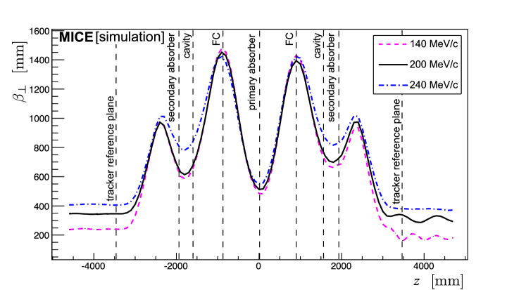
Figure 6: $\beta_{\perp}$ versus the longitudinal coordinate $z$ for 200 MeV/$c$ (solid black line), 140 MeV/$c$ (dashed purple line) and 240 MeV/$c$ (dot-dashed blue line) in the cooling-demonstration lattice. The vertical dashed lines with labels show the positions of the tracker reference planes and the centres of the absorbers, RF cavities and focus coil modules.

Table 4: Beta-function values at relevant positions for an initial beam at 140 MeV/$c$, 200 MeV/$c$ and 240 MeV/$c$ in the cooling-demonstration lattice design.

Parameter	Value for	Value for	Value for
	140 MeV/$c$	200 MeV/$c$	240 MeV/$c$
$\beta_{\perp}$ at primary absorber [mm]	480	512	545
$\beta_{\perp}$ at upstream secondary absorber [mm]	660	710	840
$\beta_{\perp}$ at downstream secondary absorber [mm]	680	740	850
$\beta_{\perp\mathrm{max}}$ at FC [mm]	1480	1450	1430

5 Simulation

Simulations to evaluate the performance of the lattice have been performed using the official MICE simulation and reconstruction software MAUS (MICE Analysis User Software) [38]. In addition to simulation, MAUS also provides a framework for data analysis. MAUS is used for offline analysis and to provide fast real-time detector reconstruction and data visualisation during MICE running. MAUS uses GEANT4 [39, 40] for beam propagation and the simulation of detector response. ROOT [41] is used for data visualisation and for data storage.

Particle tracking has been performed for several configurations. The parameters of the initial beam configurations used for the simulations are summarised in table 1. The simulation of the beam starts at a point between the diffuser and the first plane of the tracker. The beam is generated by a randomising algorithm with a fixed seed. The number of particles launched for each simulation is a compromise between the statistical uncertainty required ($\approx 1$%) and computing time. Each cavity is simulated by a TM₀₁₀ ideal cylindrical pillbox with a peak effective gradient matched to that expected for the real cavities. The reference particle is used to set the phase of the cavities so that it is accelerated “on crest”. The initial distributions defined in table 1 are centred on the reference particle in both time and momentum. Table 5 lists the acceptance criteria applied to all analyses presented here. Trajectories that fail to meet the acceptance criteria are removed from the analysis.

Table 5: Acceptance criteria for analysis.

Parameter		Acceptance condition
Particle		muon $\mu^{+}$
Transmission: pass through two planes		$z=-4600$ mm and $z=5000$ mm
Radius at $z=-4600$ mm		$\leq 150.0$ mm
Radius at $z=5000$ mm		$\leq 150.0$ mm

The normalised transverse emittance is calculated by taking the fourth root of the determinant of the four-dimensional phase-space covariance matrix [20, 21]. The MICE collaboration plans to take data such that the statistical uncertainty on the relative change in emittance for a particular setting is 1%. The MICE instrumentation was designed such that the systematic uncertainty related to the reconstruction of particle trajectories would contribute at the $\sim 0.3$% level to the overall systematic uncertainty [15]; such uncertainties would thus be negligible.

6 Performance

Figure 7 shows the evolution of the mean energy of a muon beam as it traverses the lattice. Beams with initial normalised transverse emittance $\varepsilon_{\perp}=4.2\,\text{mm}$, $\varepsilon_{\perp}=6\,\text{mm}$ and $\varepsilon_{\perp}=7.2\,\text{mm}$ for initial muon beam momenta of 140 MeV/$c$, 200 MeV/$c$ and 240 MeV/$c$ respectively are shown. The initial normalised transverse emittance is chosen such that the geometrical emittance of the three beams is the same. A 200 MeV/$c$ muon passing through two 32.5 mm thick secondary LiH absorbers and one 65 mm thick primary LiH absorber loses an energy of 18.9 MeV. Including losses in the scintillating-fibre trackers and windows, this increases to 24.3 MeV. The accelerating gradient that can be achieved in each of the two cavities is constrained by the available RF power and is insufficient to replace all the lost energy. Therefore, a comparison of beam energy with and without acceleration is required. With acceleration an energy deficit of $\langle\Delta E\rangle=19$ MeV will be observed. This measurable difference will be used to extrapolate the measured cooling effect to that which would pertain if all the lost energy were restored.

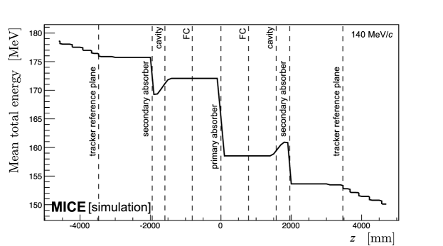
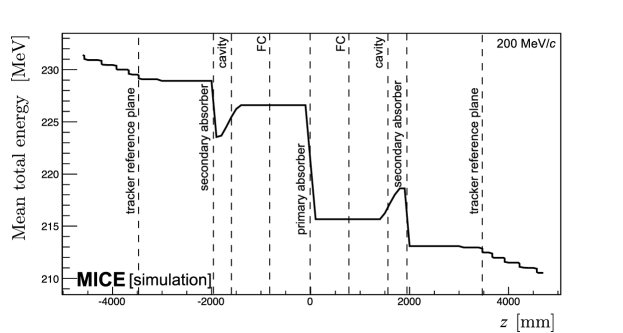
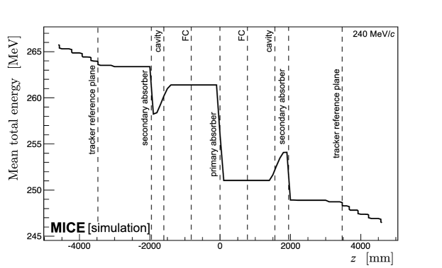
Figure 7: Mean energy of the beam versus longitudinal coordinate ($z$) in the cooling-demonstration lattice. Top: the 140 MeV/$c$ configuration for initial emittance $\varepsilon_{\perp}=4.2\,\text{mm}$. Middle: the 200 MeV/$c$ configuration for initial emittance $\varepsilon_{\perp}=6\,\text{mm}$. Bottom: the 240 MeV/$c$ configuration for initial emittance $\varepsilon_{\perp}=7.2\,\text{mm}$. The vertical dashed lines with labels show the positions of the tracker reference planes, and the centres of the absorbers, RF cavities and focus-coil modules.

The evolution of normalised transverse emittance across the lattice is shown in figure 8. The beam is subject to non-linear effects in regions of high $\beta_{\perp}$, which cause the normalised transverse emittance to grow, especially in the 140 MeV/$c$ configuration. This phenomenon can be seen in three different regions of the lattice: a moderate increase in emittance is observed at $z\approx-2500$ mm and $z\approx 1000$ mm while a larger increase is observed at $z\approx 3000$ mm. The non-linear effects are mainly chromatic in origin, since they are greatly lessened when the initial momentum spread is reduced. This is illustrated for the 140 MeV/c case for which the evolution of normalised emittance for beams with an rms momentum spread of 6.7 MeV/c and 2.5 MeV/c are shown. Nonetheless, in all cases a reduction in emittance is observed between the upstream and downstream trackers ($z=\pm 3473$ mm). The lattice is predicted to achieve an emittance reduction between the tracker reference planes of $\approx 8.1$%, $\approx 5.8$% and $\approx 4.0$% in the 140 MeV/$c$, 200 MeV/$c$ and 240 MeV/$c$ cases, respectively. A reduction as large as $\approx 10$% can be reached in the 140 MeV/$c$ configuration with an rms momentum spread of 1.4%.

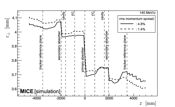
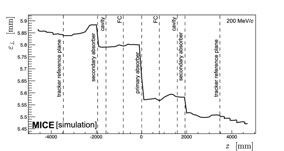
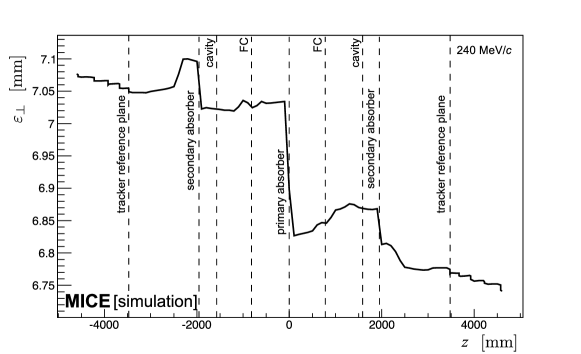
Figure 8: Emittance variation versus the longitudinal coordinate ($z$) for the cooling-demonstration lattice design. Top: 140 MeV/c beam with initial $\varepsilon_{\perp}=4.2\,\text{mm}$ with an rms momentum spread of 6.7 MeV/$c$ (rms spread $4.8\%$, solid line) and 2.5 MeV/$c$ (rms spread $1.8\%$, dashed line). Middle: 200 MeV/c beam with initial $\varepsilon_{\perp}=6\,\text{mm}$ (rms spread $4.0\%$). Bottom: 240 MeV/c beam with initial $\varepsilon_{\perp}=7.2\,\text{mm}$ (rms spread $3.6\%$). The vertical dashed lines with labels show the positions of the tracker reference planes, and the centres of the absorbers, RF cavities and focus coil modules.

The transmission of the cooling-demonstration lattice for beams of mean momentum 140 MeV/c, 200 MeV/c and 240 MeV/c is shown in figure 9. Transmission is computed as the ratio of the number of particles that satisfy the acceptance criteria observed downstream of the cooling cell divided by the number that enter the cell. This accounts for decay losses and implies that, in the absence of scraping or acceptance losses, the maximum transmission for beams of mean momentum 140 MeV/c, 200 MeV/c and 240 MeV/c is 98.9%, 99.2% and 99.5% respectively. The lattice delivers transmission close to the maximum for 200 MeV/c and 240 MeV/c beams with input emittance below $\approx 5$ mm and $\approx 7$ mm respectively. For beams of larger input emittance, the transmission gradually decreases with increasing initial emittance due to the scraping of high amplitude muons. The beam is subject to chromatic effects in regions of high $\beta_{\perp}$, which causes non-linear emittance growth. The behaviour of the transmission for the various beam energies results from the different geometrical emittance values of the beam for the same initial normalised emittance and the energy dependence of the energy loss and scattering in the material through which the beam passes.

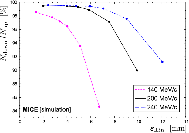
Figure 9: Transmission (defined as the ratio of good muons observed downstream of the cooling cell, $N_{\rm down}$, to those observed upstream, $N_{\rm up}$) in percent versus initial emittance ($\varepsilon_{\perp{\rm in}}$) for the cooling-demonstration lattice. The transmission of the 140 MeV/c, 200 MeV/c and 240 MeV/c lattices are shown as the purple-dashed, solid black, and dot-dashed blue lines respectively.

The fractional change in normalised transverse emittance with respect to the input emittance for beams of mean momentum 140 MeV/$c$, 200 MeV/$c$ and 240 MeV/$c$ is shown in figure 10. The different values of the equilibrium emittance and the asymptote at large emittance for each momentum are clearly visible in figure 10. A maximum cooling effect of 15%, 8% and 6% can be observed for beams with 140 MeV/$c$, 200 MeV/$c$ and 240 MeV/$c$, respectively.

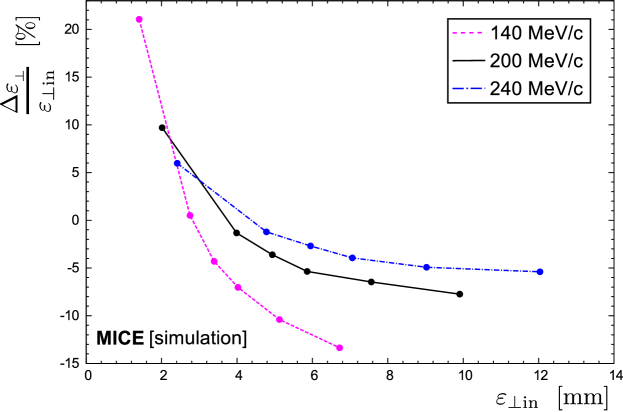
Figure 10: Fractional change in emittance versus initial emittance ($\varepsilon_{\perp{\rm in}}$) for the cooling-demonstration lattice design measured at the tracker reference planes. The fractional change in emittance of the 140 MeV/c, 200 MeV/c and 240 MeV/c lattices are shown as the purple-dashed, solid black, and dot-dashed blue lines respectively.

7 Conclusion

An experiment by which to demonstrate ionization cooling has been described that is predicted by simulations to exhibit cooling over a range of momentum. The demonstration is performed using lithium-hydride absorbers and with acceleration provided by two 201 MHz cavities. The equipment necessary to mount the experiment is either in hand (the superconducting magnets and instrumentation), or at an advanced stage of preparation. The configuration of the demonstration of ionization cooling has been shown to deliver the performance required for the detailed study of the ionization-cooling technique.

The demonstration of ionization cooling is essential to the future development of muon-based facilities that would provide the intense, well characterised low-emittance muon beams required to elucidate the physics of flavour at a neutrino factory or to deliver multi-TeV lepton-antilepton collisions at a muon collider. The successful completion of the MICE programme would therefore herald the establishment of a new technique for particle physics.

M. Bogomilov, R. Tsenov, G. Vankova-Kirilova
Department of Atomic Physics, St. Kliment Ohridski University of Sofia, Sofia, Bulgaria

Y. Song, J. Tang
Institute of High Energy Physics, Chinese Academy of Sciences, Beijing, China

Z. Li
Sichuan University, China

R. Bertoni, M. Bonesini, F. Chignoli, R. Mazza
Sezione INFN Milano Bicocca, Dipartimento di Fisica G. Occhialini, Milano, Italy

V. Palladino
Sezione INFN Napoli and Dipartimento di Fisica, Università Federico II, Complesso Universitario di Monte S. Angelo, Napoli, Italy

A. de Bari, G. Cecchet
Sezione INFN Pavia and Dipartimento di Fisica, Pavia, Italy

D. Orestano, L. Tortora
INFN Sezione di Roma Tre and Dipartimento di Matematica e Fisica, Università Roma Tre, Italy

Y. Kuno
Osaka University, Graduate School of Science, Department of Physics, Toyonaka, Osaka, Japan

S. Ishimoto
High Energy Accelerator Research Organization (KEK), Institute of Particle and Nuclear Studies, Tsukuba, Ibaraki, Japan

F. Filthaut
Nikhef, Amsterdam, The Netherlands and Radboud University, Nijmegen, The Netherlands

D. Jokovic, D. Maletic, M. Savic
Institute of Physics, University of Belgrade, Serbia

O. M. Hansen, S. Ramberger, M. Vretenar
CERN, Geneva, Switzerland

R. Asfandiyarov, A. Blondel, F. Drielsma, Y. Karadzhov
DPNC, Section de Physique, Université de Genève, Geneva, Switzerland

G. Charnley, N. Collomb, K. Dumbell, A. Gallagher, A. Grant, S. Griffiths, T. Hartnett, B. Martlew, A. Moss, A. Muir, I. Mullacrane, A. Oates, P. Owens, G. Stokes, P. Warburton, C. White
STFC Daresbury Laboratory, Daresbury, Cheshire, UK

D. Adams, R.J. Anderson, P. Barclay, V. Bayliss, J. Boehm, T. W. Bradshaw, M. Courthold, V. Francis, L. Fry, T. Hayler, M. Hills, A. Lintern, C. Macwaters, A. Nichols, R. Preece, S. Ricciardi, C. Rogers, T. Stanley, J. Tarrant, M. Tucker, A. Wilson
STFC Rutherford Appleton Laboratory, Harwell Oxford, Didcot, UK

S. Watson
STFC Rutherford UK Astronomy Technology Centre, Royal Observatory, Edinburgh, Blackford Hill, Edinburgh EH9 3HJ, UK

R. Bayes, J. C. Nugent, F. J. P. Soler
School of Physics and Astronomy, Kelvin Building, The University of Glasgow, Glasgow, UK

R. Gamet
Department of Physics, University of Liverpool, Liverpool, UK

G. Barber, V. J. Blackmore, D. Colling, A. Dobbs, P. Dornan, C. Hunt, A. Kurup, J-B. Lagrange, K. Long, J. Martyniak, S. Middleton, J. Pasternak, M. A. Uchida
Department of Physics, Blackett Laboratory, Imperial College London, London, UK

J. H. Cobb, W. Lau
Department of Physics, University of Oxford, Denys Wilkinson Building, Oxford, UK

C. N. Booth, P. Hodgson, J. Langlands, E. Overton, M. Robinson, P. J. Smith, S. Wilbur
Department of Physics and Astronomy, University of Sheffield, Sheffield, UK

A. J. Dick, K. Ronald, C. G. Whyte, A. R. Young
SUPA and the Department of Physics, University of Strathclyde, Glasgow, UK and Cockroft Institute, UK

S. Boyd, P. Franchini, J. R. Greis, C. Pidcott, I. Taylor
Department of Physics, University of Warwick, Coventry, UK

R.B.S. Gardener, P. Kyberd, J. J. Nebrensky
Brunel University, Uxbridge, UK

M. Palmer, H. Witte
Brookhaven National Laboratory, NY, USA

A. D. Bross, D. Bowring, A. Liu, D. Neuffer, M. Popovic, P. Rubinov
Fermilab, Batavia, IL, USA

A. DeMello, S. Gourlay, D. Li, S. Prestemon, S. Virostek
Lawrence Berkeley National Laboratory, Berkeley, CA, USA

B. Freemire, P. Hanlet, D. M. Kaplan, T. A. Mohayai, D. Rajaram, P. Snopok, V. Suezaki, Y. Torun
Illinois Institute of Technology, Chicago, IL, USA

Y. Onel
Department of Physics and Astronomy, University of Iowa, Iowa City, IA, USA

L. M. Cremaldi, D. A. Sanders, D. J. Summers
University of Mississippi, Oxford, MS, USA

G. G. Hanson, C. Heidt
University of California, Riverside, CA, USA

References

- [1] S. Geer, “Neutrino beams from muon storage rings: Characteristics and physics potential,” Phys. Rev. D57 (1998) 6989–6997, arXiv:hep-ph/9712290.
- [2] M. Apollonio et al., “Oscillation physics with a neutrino factory,” arXiv:hep-ph/0210192 [hep-ph].
- [3] D. V. Neuffer and R. B. Palmer, “A High-Energy High-Luminosity Collider,” in 4th European Particle Accelerator Conference (EPAC 94) London, England, June 27-July 1, 1994, vol. C940627, pp. 52–54. 1995.
- [4] R. B. Palmer, “Muon Colliders,” Rev. Accel. Sci. Tech. 7 (2014) 137–159.
- [5] S. Y. Lee, Accelerator Physics (Third Edition). World Scientific Publishing Co, 2012.
- [6] S. Schröder, R. Klein, N. Boos, M. Gerhard, R. Grieser, G. Huber, A. Karafillidis, M. Krieg, N. Schmidt, T. Kühl, R. Neumann, V. Balykin, M. Grieser, D. Habs, E. Jaeschke, D. Krämer, M. Kristensen, M. Music, W. Petrich, D. Schwalm, P. Sigray, M. Steck, B. Wanner, and A. Wolf, “First laser cooling of relativistic ions in a storage ring,” Phys. Rev. Lett. 64 (Jun, 1990) 2901–2904. http://link.aps.org/doi/10.1103/PhysRevLett.64.2901.
- [7] J. S. Hangst, M. Kristensen, J. S. Nielsen, O. Poulsen, J. P. Schiffer, and P. Shi, “Laser cooling of a stored ion beam to 1 mk,” Phys. Rev. Lett. 67 (Sep, 1991) 1238–1241. http://link.aps.org/doi/10.1103/PhysRevLett.67.1238.
- [8] P. J. Channell, “Laser cooling of heavy ion beams,” Journal of Applied Physics 52 no. 6, (1981) 3791–3793, http://dx.doi.org/10.1063/1.329218. http://dx.doi.org/10.1063/1.329218.
- [9] J. Marriner, “Stochastic cooling overview,” Nucl. Instrum. Meth. A532 (2004) 11–18, arXiv:physics/0308044 [physics].
- [10] V. V. Parkhomchuk and A. N. Skrinsky, “Electron cooling: 35 years of development,” Physics-Uspekhi 43 no. 5, (2000) 433–452. http://stacks.iop.org/1063-7869/43/i=5/a=R01.
- [11] A. N. Skrinsky and V. V. Parkhomchuk, “Cooling Methods for Beams of Charged Particles. (In Russian),” Sov. J. Part. Nucl. 12 (1981) 223–247. [Fiz. Elem. Chast. Atom. Yadra12,557(1981)].
- [12] D. Neuffer, “Principles and Applications of Muon Cooling,” in Proceedings, 12th International Conference on High-Energy Accelerators, HEACC 1983: Fermilab, Batavia, August 11-16, 1983, vol. C830811, pp. 481–484. 1983.
- [13] D. Neuffer, “Principles and Applications of Muon Cooling,” Part. Accel. 14 (1983) 75–90.
- [14] D. Rajaram and V. C. Palladino, “The Status of MICE Step IV,” in Proceedings, 6th International Particle Accelerator Conference (IPAC 2015): Richmond, Virginia, USA, May 3-8, 2015, pp. 4000–4002. 2015. http://accelconf.web.cern.ch/AccelConf/IPAC2015/papers/thpf122.pdf.
- [15] MICE Collaboration, “MICE: An International Muon Ionization Cooling Experiment.” http://mice.iit.edu/micenotes/public/pdf/MICE0021/MICE0021.pdf, 2003. MICE Note 21.
- [16] ISS Accelerator Working Group Collaboration, M. Apollonio et al., “Accelerator design concept for future neutrino facilities,” JINST 4 (2009) P07001, arXiv:0802.4023 [physics.acc-ph].
- [17] C. M. Ankenbrandt et al., “Status of muon collider research and development and future plans,” Phys. Rev. ST Accel. Beams 2 (1999) 081001, arXiv:physics/9901022 [physics].
- [18] Neutrino Factory and Muon Collider Collaboration, M. M. Alsharoa et al., “Recent progress in neutrino factory and muon collider research within the Muon collaboration,” Phys. Rev. ST Accel. Beams 6 (2003) 081001, arXiv:hep-ex/0207031 [hep-ex].
- [19] R. B. Palmer, J. S. Berg, R. C. Fernow, J. C. Gallardo, H. G. Kirk, Y. Alexahin, D. Neuffer, S. A. Kahn, and D. Summers, “A Complete Scheme of Ionization Cooling for a Muon Collider,” in Particle accelerator. Proceedings, 22nd Conference, PAC’07, Albuquerque, USA, June 25-29, 2007, vol. C070625, pp. 3193–3195. 2007. arXiv:0711.4275 [physics.acc-ph].
- [20] G. Penn and J. S. Wurtele, “Beam envelope equations for cooling of muons in solenoid fields,” Phys. Rev. Lett. 85 (2000) 764.
- [21] C. Rogers, Beam Dynamics in an Ionisation Cooling Channel. PhD dissertation, Imperial College of London, 2008.
- [22] D. Stratakis and R. B. Palmer, “Rectilinear six-dimensional ionization cooling channel for a muon collider: A theoretical and numerical study,” Phys. Rev. ST Accel. Beams 18 no. 3, (2015) 031003.
- [23] D. Neuffer, H. Sayed, T. Hart, and D. Summers, “Final Cooling for a High-Energy High-Luminosity Lepton Collider,” Submitted to: JINST (2015) , arXiv:1612.08960 [physics.acc-ph].
- [24] A. V. Tollestrup and J. Monroe, “Multiple Scattering Calculations for Hydrogen, Helium, Lithium, and Beryllium,” Tech. Rep. FERMILAB-MUCOOL-176, Fermi National Accelerator Laboratory, 2000.
- [25] C. N. Booth et al., “The design, construction and performance of the MICE target,” JINST 8 (2013) P03006, arXiv:1211.6343 [physics.ins-det].
- [26] C. N. Booth et al., “The design and performance of an improved target for MICE,” JINST 11 no. 05, (2016) P05006, arXiv:1603.07143 [physics.ins-det].
- [27] MICE Collaboration, M. Bogomilov et al., “The MICE Muon Beam on ISIS and the beam-line instrumentation of the Muon Ionization Cooling Experiment,” JINST 7 (2012) P05009, arXiv:1203.4089 [physics.acc-ph].
- [28] MICE Collaboration, D. Adams et al., “Characterisation of the muon beams for the Muon Ionisation Cooling Experiment,” Eur. Phys. J. C73 no. 10, (2013) 2582, arXiv:1306.1509 [physics.acc-ph].
- [29] R. Bertoni et al., “The design and commissioning of the MICE upstream time-of-flight system,” Nucl. Instrum. Meth. A615 (2010) 14–26, arXiv:1001.4426 [physics.ins-det].
- [30] R. Bertoni, M. Bonesini, A. de Bari, G. Cecchet, Y. Karadzhov, and R. Mazza, “The construction of the MICE TOF2 detector.” http://mice.iit.edu/micenotes/public/pdf/MICE0286/MICE0286.pdf, 2010.
- [31] L. Cremaldi, D. A. Sanders, P. Sonnek, D. J. Summers, and J. Reidy, Jr, “A Cherenkov Radiation Detector with High Density Aerogels,” IEEE Trans. Nucl. Sci. 56 (2009) 1475–1478, arXiv:0905.3411 [physics.ins-det].
- [32] M. Ellis et al., “The design, construction and performance of the MICE scintillating fibre trackers,” Nucl. Instrum. Meth. A659 (2011) 136–153, arXiv:1005.3491 [physics.ins-det].
- [33] F. Ambrosino et al., “Calibration and performances of the KLOE calorimeter,” Nucl. Instrum. Meth. A598 (2009) 239–243.
- [34] R. Asfandiyarov et al., “The design and construction of the MICE Electron-Muon Ranger,” JINST 11 no. 10, (2016) T10007, arXiv:1607.04955 [physics.ins-det].
- [35] M. Leonova et al., “MICE Cavity Installation and Commissioning/Operation at MTA,” in Proceedings, 6th International Particle Accelerator Conference (IPAC 2015): Richmond, Virginia, USA, May 3-8, 2015, pp. 3342–3344. 2015. http://accelconf.web.cern.ch/AccelConf/IPAC2015/papers/wepty032.pdf.
- [36] Y. Torun et al., “Final Commissioning of the MICE RF Module Prototype with Production Couplers,” in Proceedings, 7th International Particle Accelerator Conference (IPAC 2016): Busan, Korea, May 8-13, 2016, pp. 474–476. 2016. http://inspirehep.net/record/1469641/files/mopmw034.pdf.
- [37] R. C. Fernow and R. B. Palmer, “Solenoidal ionization cooling lattices,” Phys. Rev. ST Accel. Beams 10 (Jun, 2007) 064001. http://link.aps.org/doi/10.1103/PhysRevSTAB.10.064001.
- [38] C. D. Tunnell and C. T. Rogers, “MAUS: MICE Analysis User Software,” in Particle accelerator. Proceedings, 2nd International Conference, IPAC 2011, San Sebastian, Spain, September 4-9, 2011, vol. C110904, pp. 850–852. 2011.
- [39] GEANT4 Collaboration, S. Agostinelli et al., “Geant4: A simulation toolkit,” Nucl. Instrum. Meth. A506 (2003) 250–303.
- [40] J. Allison et al., “Geant4 developments and applications,” IEEE Trans. Nucl. Sci. 53 (2006) 270–278.
- [41] R. Brun and F. Rademakers, “ROOT: An object oriented data analysis framework,” Nucl. Instrum. Meth. A389 (1997) 81–86.