NLO electroweak radiative corrections for four-fermionic process at Belle II

Abstract

We discuss the next to the leading order (NLO) electroweak radiative corrections to the $e^{-}e^{+}\rightarrow f^{-}f^{+}(\gamma)$ cross section asymmetry, for polarized and unpolarized beam scenario. The left-right and forward-backward amplitudes, with and without radiative corrections, are evaluated and compared for various kinematics. The hard bremsstrahlung is included for arbitrary energy cuts. The radiative corrections are shown to be significant and having a non-trivial dependency on the kinematic conditions. The calculations are relevant for the ultra-precise low-energy experiment Belle II planned at SuperKEKB.

1 Introduction

The precision electroweak physics will be accessed at low energy by the upcoming experiments such as Belle-II at SuperKEKB  BelleIITDR , MOLLER at JLab MOLLER and P2 at MESA P2 and play an important complimentary role to the direct new-physics search at the LHC. Belle II aims to determine the weak mixing angle at $\sqrt{s}=m(\Upsilon_{4S})=10.577$ GeV, with the same precision as the LEP/SLC measurements made at the $Z$-boson pole and for $e^{-}e^{+}\rightarrow b\bar{b}$ but free from fragmentation uncertainties Bevan . However, before the reliable information can be extracted from the experimental data, it is necessary to consider the higher-order effects, i.e. electroweak radiative corrections (EWC). The inclusion EWC is an indispensable part of any modern experiment, but will be of the most paramount importance for the upcoming ultra-precise measurements, and, in some cases, must include not only a full treatment of one-loop radiative corrections (NLO) but also the leading two-loop corrections (NNLO).

The significant theoretical effort has been dedicated to NLO EWC to electron-positron annihilation for more than three decades now, starting from BH82 which discussed EWC for an arbitrary polarization. Later, the collaborations such as BHM and WOH hollik ; BH84 , LEPTOP LEPTOP , TOPAZ0 TOPAZ96 and ZFITTER ZF91 ; grup-bar2 , provided a new level of precision for EWC at the $Z$-pole required by the LEP and SLC colliders. More recent EWC of the post-LEP/SLC era are offered by KK KK and SANC sanc-eeff codes. Although quick and accessible, these generic “ready-to-use” codes may not be optimal for the new generation of precision experiments requiring a more custom approach. The previous work by our theory group ABIZ2010ABIKZ2013 dedicated to the parity-violating (PV) tests of the Standard Model showed that the exact analytical one-loop calculations using the computer algebra approach did not only increase the theoretical precision dramatically, but also gave us an opportunity to verify previous calculations done in other formalisms 13-Au . A more detailed analysis of the low- and high-energy asymptotic behavior of electroweak radiative corrections in polarized $e^{-}e^{+}\to\mu^{-}\mu^{+}$ process can be found in ABBZ2016 .

The main goal of this paper is to calculate a full gauge-invariant set of NLO EWC, both with computer algebra requiring no simplifications, using our semi-automatic approach (SAA) based on FeynArts, FormCalc and LoopTools Hahn , and analytically (on paper), in a compact form, using the asymptotic methods hollik ; 13-Au , and to compare the results making sure that our calculations are error-free. A complete set of NNLO EWC is not yet available and not included in the current analysis, but the work is already in progress by several groups (for example, UsNNLO2016 and RHill2016 ) and planned to be completed in time for the upcoming experiments such as Belle II, MOLLER and P2.

2 NLO electroweak corrections

Let us start by defining the cross section for scattering of polarized electrons on unpolarized positrons,

$$e^{-}(p_{1})+e^{+}(p_{2})\rightarrow f^{-}(p_{3})+f^{+}(p_{4}).$$ (1)

In the Born approximation (leading order) illustrated by the first diagram in Fig. 1, we have: $\sigma^{0}\approx\frac{\pi^{3}}{2s}|M_{0}|^{2}$.

Figure 1: Feynman diagrams for the $e^{-}e^{+}\rightarrow\mu^{-}\mu^{+}$ process in radiation-free kinematics

Here, $\sigma$ is the differential cross section $\sigma\equiv{d\sigma}/{d(\cos\theta)}$, $\theta$ is the scattering angle of the detected muon with 4-momentum $p_{3}$ in the center-of-mass system of the initial electron and positron, and $M_{0}$ is the Born (${\cal O}(\alpha)$) amplitude (matrix element). The 4-momenta of initial ($p_{1}$ and $p_{2}$) and final ($p_{3}$ and $p_{4}$) fermions generate a standard set of Mandelstam variables:

$$s=(p_{1}+p_{2})^{2},\ t=(p_{1}-p_{3})^{2},\ u=(p_{1}-p_{4})^{2}.$$ (2)

At the Next-to-Leading-Order (${\cal O}(\alpha^{2})$), the differential cross section is given by the second term of the following expansion:

$$\sigma=\frac{\pi^{3}}{2s}|M_{0}+M_{1}|^{2}\approx\frac{\pi^{3}}{2s}(M_{0}M_{0}^{+}+2{\rm Re}[M_{1}M_{0}^{+}]),$$ (3)

where the one-loop amplitude $M_{1}$ is the sum of boson self-energy (BSE), vertex (Ver) and box diagrams (see Fig. 1):

$$M_{1}=M_{{\rm BSE}}+M_{{\rm Ver}}+M_{{\rm Box}}.$$ (4)

There are no contributions from the electron self-energies in the on-shell renormalization scheme BSH86 ; Denner . The explicit form of the Born and one-loop amplitudes can be found in Yaf16 .

The bremsstrahlung diagrams corresponding to initial state radiation (ISR) and the final state radiation (FSR) are illustrated in Fig. 2.

Figure 2: Diagrams with photon emission

The differential cross section for the process

$$e^{-}(p_{1})+e^{+}(p_{2})\rightarrow f^{-}(p_{3})+f^{+}(p_{4})+\gamma(p),$$ (5)

has a form

$$d\sigma_{R}=\frac{\alpha^{3}}{\pi^{2}s}\sum|R|^{2}d\Gamma_{3}.$$ (6)

The amplitude $R$, the phase space of emitted photon $d\Gamma_{3}$, and explanation of infrared divergence are given in Yaf16 .

3 Analysis

For input parameters, we used $\alpha$, $m_{W}$,  $m_{Z}$, $m_{H}$ and fermionic masses from PDG14 . The light quark masses reproducing $\Delta\alpha_{had}^{(5)}(m_{Z}^{2})$=0.02757 jeger , are regulated by the hadronic vacuum polarization, which does not introduce a significant uncertainty to our results. Please see ABIZ2010ABIKZ2013 for details.

Let us start with a comparison between the asymptotic and full calculations, using two relative corrections $\delta^{\rm NLO}_{+}$ and $\delta^{\rm NLO}_{-}$:

$$\delta^{\rm NLO}_{\pm}=\frac{\sigma^{{\rm NLO}}_{L}\pm\sigma^{{\rm NLO}}_{R}}{\sigma^{0}_{L}\pm\sigma^{0}_{R}}.$$ (7)

They are additive, and allow to estimate the physical effect. The asymmetry can now be defined as:

$$\delta^{\rm NLO}_{A}=\frac{\delta^{\rm NLO}_{-}-\delta^{\rm NLO}_{+}}{1+\delta^{\rm NLO}_{+}}.$$ (8)

The comparison between two methods is illustrated in Fig. 3. For now, we apply the same cut on the soft photon emission energy as in 5-DePo , $\omega=0.05\sqrt{s}$, to be re-evaluated for each experiment specifically.

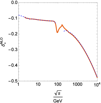
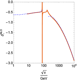
Figure 3: The relative NLO corrections at $\theta=90^{\circ}$ vs energy: solid line – computer algebra code (not working at very small $\sqrt{s}$), dashed line – asymptotic estimations, good for $\sqrt{s}$ below $m_{W}$ and for $\sqrt{s}$ above $m_{Z}$.

Let us denote the specific type of contribution in cross section or asymmetries by a subscript $C$. $C$ can be 0 (Born contribution), 1 (one-loop EWC contribution), or 0+1 (both), i.e. $C=\{0,1,0\!\!+\!\!1\}$. The PV (left-right) asymmetry, the forward-backward asymmetry, and the left-right asymmetry constructed from the integrated cross sections are defined in the traditional way:

$$A^{C}_{LR}=\frac{\sigma^{C}_{L}-\sigma^{C}_{R}}{\sigma^{C}_{L}+\sigma^{C}_{R}},\ \ \ A^{C}_{FB}=\frac{\Sigma^{C}_{F}-\Sigma^{C}_{B}}{\Sigma^{C}_{F}+\Sigma^{C}_{B}},\ \ \ A^{C}_{LR\Sigma}=\frac{\Sigma^{C}_{L}-\Sigma^{C}_{R}}{\Sigma^{C}_{L}+\Sigma^{C}_{R}}.$$ (9)

The subscripts $L$ and $R$ on the cross sections $\sigma\equiv{d\sigma}/{d(\cos\theta)}$ correspond to the polarization degree of the electron $p_{B}$ = $-1$ and $p_{B}$ = $+1$ respectively.

The forward and backward cross sections defined as:

$$\Sigma^{C}_{F}=\int\limits_{0}^{\cos a}\sigma^{C}_{00}\cdot d(\cos\theta),\ \ \ \Sigma^{C}_{B}=\int\limits_{-\cos a}^{0}\sigma^{C}_{00}\cdot d(\cos\theta).$$

and left and right integrated (over $a\leq\theta\leq b$ segment) cross sections are:

$$\Sigma^{C}_{L}=\int\limits_{\cos b}^{\cos a}\sigma^{C}_{L}\cdot d(\cos\theta),\ \ \ \Sigma^{C}_{R}=\int\limits_{\cos b}^{\cos a}\sigma^{C}_{R}\cdot d(\cos\theta).$$

Figs. 4-6 illustrate these asymmetries with and without the radiative effects.

Figure 4: Left: unpolarized NLO corrected (0+1), Born (0), and their difference (1) differential cross sections vs scattering angle $\theta$. Right: the polarization Born asymmetry (0) and asymmetry taking into account the NLO EWC (0+1) vs scattering angle $\theta$. Note the large contribution of EWC to $A_{LR}$ at small angles.

Figure 5: Left: unpolarized NLO corrected (0+1), Born (0), and their difference (1) total cross sections vs angle $a$. Right: the forward-backward Born asymmetry (0) and asymmetry taking into account the NLO EWC (0+1) vs angle $a$. Note the importance of EWC.

Figure 6: Left: unpolarized NLO corrected (0+1), Born (0), and their difference (1) integrated cross sections vs angle $b$ at $a=10^{\circ}$. Right: the left-right integrated Born asymmetry (0) and asymmetry taking into account the NLO EWC (0+1) vs angle $b$ at $a=10^{\circ}$.

4 Conclusions

We compare the results for the full set of one-loop EWC to left-right and forward-backward asymmetries at energies relevant for Belle II at SuperKEKB obtained by two different methods: the exact (semi-automatic, with computer algebra) and approximate (asymptotic, on paper). Both methods have their advantages and limitations, but their combination proves that our work is error-free and provided more options to the experimental community. The bremsstrahlung process is fully controlled and the soft- and hard-photon approximations are compared. Although much improved in this work, the precision obtained with one-loop EWC is still insufficient for the upcoming experiments such as Belle II, MOLLER and P2 and will require at least the leading two-loop contributions.

5 ACKNOWLEDGMENTS

We are grateful to the organizers of Baldin ISHEPP XXIII Seminar for hospitality and to Yu. Bystritskiy, and J.M. Roney for stimulating discussions. V.Z. thanks Harrison McCain Foundation for support and the Acadia University for hospitality in 2016. The work of A.A. and S.B. is supported by the Natural Science and Engineering Research Council of Canada (NSERC).

References

- (1) Belle II Technical Design Report, Belle II Collaboration: T. Abe et al., arXiv:1011.0352 (2010).
- (2) MOLLER Collab. (J. Benesch et al.) arXiv:1411.4088 [nucl-ex] JLAB-PHY-14-1986 (2014).
- (3) N. Berger et al., Proceedings of the PhiPsi15, Sep. 23-26, 2015, Hefei, China (2015).
- (4) A. Bevan, arXiv:1112.1394v1 [hep-ex].
- (5) M. Böhm and W. Hollik, Nucl. Phys. B 204, 45 (1982).
- (6) W. Hollik, Fortschr. Phys. 38, 165 (1990).
- (7) M. Bohm and W. Hollik, Z. Phys. C 23, 31 (1984).
- (8) V.A. Novikov, L.B. Okun, M.I. Vysotsky, Nucl. Phys. B 397, 35 (1993).
- (9) G. Montagna et al., Comput. Phys. Commun. 117, 278 (1999).
- (10) D. Bardin et al., Comput. Phys. Commun. 133, 229 (2001).
- (11) D.Yu. Bardin, S. Rieman, T. Rieman, Z. Phys. 32, 121 (1986).
- (12) S. Jadach, B.F.L. Ward and Z. Was, Phys. Rev. D 63, 113009 (2001).
- (13) A. Andonov et al., Phys. Part. Nucl. 34, 1125 (2003).
- (14) A. Aleksejevs et al., Phys. Rev. D 82, 093013 (2010); Phys. Part. Nucl. 44, 161 (2013).
- (15) V.A. Zykunov, Phys. Rev. D 75, 073019, (2007).
- (16) A. Aleksejevs et al., arXiv:1609.08666 (2016).
- (17) T. Hahn, M. Perez-Victoria, Comput. Phys. Commun. 118, 153 (1999).
- (18) A. Aleksejevs et al., Phys. Part. Nuclei Lett. 13, 310 (2016).
- (19) Richard J. Hill, arXiv:1605.02613 (2016).
- (20) M. Böhm, H. Spiesberger, and W. Hollik, Fortschr. Phys. 34, 687 (1986).
- (21) A. Denner, Fortsch. Phys. 41, 307 (1993).
- (22) A.G. Aleksejevs, S.G. Barkanova, V.A. Zykunov, Phys. Atom. Nucl. 79, 78 (2016).
- (23) K. A. Olive et al. (Particle Data Group), Chin. Phys. C 38, 090001 (2014).
- (24) F. Jegerlehner, J. Phys. G. 29 101 (2003) [hep-ph/0104304].
- (25) A. Denner and S. Pozzorini, Eur. Phys. J. C 7, 185 (1999).