Frequency analysis and the representation of slowly diffusing planetary solutions

Abstract

Context. Over short time intervals planetary ephemerides have been traditionally represented in analytical form as finite sums of periodic terms or sums of Poisson terms that are periodic terms with polynomial amplitudes. Nevertheless, this representation is not well adapted for the evolution of the planetary orbits in the solar system over million of years as they present drifts in their main frequencies, due to the chaotic nature of their dynamics.

Aims. The aim of the present paper is to develop a numerical algorithm for slowly diffusing solutions of a perturbed integrable Hamiltonian system that will apply to the representation of the chaotic planetary motions with varying frequencies.

Methods. By simple analytical considerations, we first argue that it is possible to recover exactly a single varying frequency. Then, a function basis involving time-dependent fundamental frequencies is formulated in a semi-analytical way. Finally, starting from a numerical solution, a recursive algorithm is used to numerically decompose the solution on the significant elements of the function basis.

Results. Simple examples show that this algorithm can be used to give compact representations of different types of slowly diffusing solutions. As a test example, we show how this algorithm can be successfully applied to obtain a very compact approximation of the La2004 solution of the orbital motion of the Earth over 40 Myr ([-35Myr,5Myr]). This example has been chosen as this solution is widely used for the reconstruction of the climates of the past.

1 Introduction

Before the computer ages, the long term solutions for the planetary orbits were derived by perturbation methods, and obtained in the form of sum of periodic terms. The first of such solutions was obtained by Lagrange (1782) who only considered the known planets of the time, that is the planets that are visible by naked eye (Mercury, Venus, Earth, Mars, Jupiter and Saturn). This was later on improved by LeVerrier (1840, 1841) who took also Uranus into account. These long term solutions have revealed to be of fundamental importance for the understanding of the past climate of the Earth, when it was understood that the changes of the orbit of the Earth induce also some change in its obliquity and in the insolation at the Earth surface (Milankovitch, 1941) (for a detailed review, see Laskar et al. (2004)). With the advent of computers, two different approaches become possible. Computer algebra allowed to extend the perturbation methods (e.g. Bretagnon, 1974), and as the computer speed increased, direct integrations of the full Solar system become possible (Quinn et al., 1991; Sussman & Wisdom, 1992). Meanwhile, Laskar (1985, 1986, 1988) developed a mixed strategy, with an analytical averaging of the planetary equations obtained by perturbation methods using dedicated computer algebra. This analytical averaging was then followed by a numerical integration of the averaged system with high order multistep method. In order to compare the output of the numerical integrations with the quasiperiodic solutions of the perturbative methods, Laskar (1988) introduced the frequency analysis method that allowed to obtain in a very efficient way a precise approximation of the numerical solution in quasiperiodic form (e.g. Laskar (2005)).

But although the goal was to search for the most precise long term solution for the planetary orbits, one of the outcomes of these computations was to demonstrate that the solar system motion is chaotic (Laskar, 1989, 1990). As a consequence, the solutions are not quasiperiodic, although they can be approximated by a quasiperiodic expression over a limited time of a few million of years (Laskar, 1988, 1990; Laskar et al., 2004).

In the present work, we derive a more adapted strategy for the slowly diffusing trajectories of a dynamical system that will be very well suited to the construction of compact forms for the long time behaviour of the planetary orbits. We introduce an algorithm, that is derived from the frequency analysis, but where a slow variation of the frequencies and amplitudes is added. Here, by a slowly diffusing solution, we mean a solution that, while experiencing significant frequency drifts in the whole considered time interval, is nearly quasiperiodic in time subintervals. Similar to frequency analysis, a key step of our algorithm is to construct frequency-dependent function basis on which the considered solution will be decomposed.

In section 2, after reminding some fundamental results on frequency analysis, we consider a single term model and show that it is possible to recover exactly its varying frequency as a function of time. This is important when one is interested in the details of how a solution diffuses in the frequency space. But for constructing a compact solution representation with a reasonably high precision, small flickers without significant cumulative effects can be smoothed out from a varying frequency. Therefore, it is preferable to use a model with limited number of parameters, e.g. low-order polynomials, to approximate the frequency. To do so, we sample the average frequencies over a sliding time interval. For a slowly diffusing solution, it is assumed that all fundamental frequencies can be sampled in this way by using the NAFF algorithm (e.g. (Laskar, 2005)).

In section 3, a general algorithm of representing a slowly diffusing solution is designed, where a frequency-dependent function basis is constructed based on the Chebyshev approximations of fundamental frequencies. The basis functions with significant but non-fundamental frequencies are generated according to the assumption that, at any instant, a slowly diffusing solution is nearly quasi-periodic with the smoothed fundamental frequencies at that instant, namely all main frequencies are integral linear combinations of the fundamental frequencies. This effectively avoids the difficulties in determining the frequencies of long-period terms and/or groups of neighboring-period terms.

Two simple examples are given in section 4. In the first example, a weakly dissipated system is considered, and the represented solution diffuses because of dissipation. In the second example, a Hamiltonian system of degree 1.5 is considered, and a solution starting from an obvious resonance overlap zone is represented. To show the flexibility of our algorithm in representing such a solution, we exclude all possible libration frequencies from the set of fundamental frequencies used in constructing the function basis.

Applications to the representation of ephemerides of the solar system bodies are provided in section 5. As examples, the eccentricity and the inclination of the Earth, as given by the long-term numerical solution La2004 (Laskar et al., 2004), are represented. For such a realistic solution, it is natural to take into account the restrictions on the representation model from previous results, e.g. the important libration frequencies from numerical analysis (e.g. Laskar et al., 2004), so that the resulting representations can be as close as possible to the physical model.

2 Frequency analysis and time-dependent frequencies

For a KAM solution of a dynamical system (Kolmogorov, 1954; Arnol’d, 1963; Moser, 1962), with fundamental frequency vector $\mathbf{\nu}=(\nu_{1},...,\nu_{N})\in R^{N}$, where $N$ is the number of degrees of freedom of the system, the motion of any given degree of freedom, with associated variable $z(t)$, can be described in complex form as

$$z(t)=\sum_{\mathbf{k}\in Z^{N}}a_{\mathbf{k}}{\rm e}^{{\rm i}\langle\mathbf{k},\mathbf{\nu}\rangle t},$$ (1)

where $\mathbf{k}=(k_{1},...,k_{N})$ is the frequency index vector, $a_{\mathbf{k}}$ complex amplitude, and $\langle\cdot,\cdot\rangle$ denotes the usual inner product of two real vectors.

The NAFF (Numerical Analysis of Fundamental Frequencies) algorithm was designed to numerically recover significant terms of (1) from a numerical sample set of $z(t)$, e.g. an ephemeris obtained by numerical integration (Laskar, 1988). However, the application of NAFF is not limited to numerically recovering KAM solutions. Actually, most relevant works are about frequency drifts. In particular, the variations of the fundamental frequencies of the secular solar system over 200Myr was used to study the chaotic behavior of the solar system (Laskar, 1990).

Let us first recall briefly the theorem about the convergence of the NAFF algorithm (for the complete version with proof, see (Laskar, 2005)). With a set of $N$ appropriate variables, the complex function (1) describing a degree of freedom of an analytic KAM solution can be written as

$$z(t)={\rm e}^{{\rm i}\nu_{1}t}+\sum_{\mathbf{k}\in Z^{N}-(1,0,...,0)}a_{\mathbf{k}}{\rm e}^{{\rm i}\langle\mathbf{k},\mathbf{\nu}\rangle t}\ \ \ \ (|a_{\mathbf{k}}|<1),$$ (2)

where $\nu_{1}$ is a fundamental frequency. We have then (e.g. Laskar, 1999)

Theorem 1 Let $\nu_{1}^{T}$ be the value of $\sigma\in R$ that maximizes the function $\phi(\sigma)=|\langle z(t),{\rm e}^{{\rm i}\sigma t}\rangle_{T}^{\chi}|,$ where $\chi=\chi(t/T)>0$ is a weight function, and $\langle\cdot,\cdot\rangle_{T}^{\chi}$ the inner product of two complex functions of $t$ defined as

$$\langle f(t),g(t)\rangle_{T}^{\chi}=\frac{1}{2T}\int_{-T}^{T}f(t)\bar{g}(t)\chi(t/T)dt,$$ (3)

we then have $\lim_{T\rightarrow\infty}\nu_{1}^{T}=\nu_{1}$.$\square$

Similar to the fundamental frequency $\nu_{1}$, any other main frequency can be recovered by searching its neighborhood or $R$ for the value of $\sigma$ that maximizes $\phi(\sigma)$ defined with the remaining $z(t)$, that is, the original $z(t)$ minus the recovered terms.

A diffusion solution is then characterized by fundamental frequency variations (Laskar et al., 1992; Laskar, 1993). Regarding to the determination of a varying frequency, let’s first consider the following simplest case,

$$f(t)=a(t){\rm e}^{{\rm i}\int_{0}^{t}\nu(\tau)d\tau},$$ (4)

where $\nu(t)$ and $a(t)>0$ are real integrable functions. Writing

$$\phi(\sigma(t))=\left|\langle f(t),{\rm e}^{{\rm i}\int_{0}^{t}\sigma(\tau)d\tau}\rangle_{T}^{\chi}\right|=\left|\frac{1}{2T}\int_{-T}^{T}a(t){\rm e}^{{\rm i}\theta(t)}\chi(t/T)dt\right|,$$ (5)

where $\theta(t)=\int_{0}^{t}(\nu(\tau)-\sigma(\tau))d\tau$ belongs to $\mathcal{C}^{0}$, the set of continuous function on $R$, we have the following theorem

Theorem 2 For any given $T>0$ and $\nu(t)\in\mathcal{C}^{0}$, the functional $\phi(\sigma(t))$ has one and only one maximum in $\mathcal{C}^{0}$, which is attained at $\sigma(t)\equiv\nu(t)$. $\square$

Proof. The right-hand side of (5) can be written as

$$\left|\frac{1}{2T}\int_{-T}^{T}(\sqrt{a(t)})(\sqrt{a(t)}{\rm e}^{{\rm i}\theta(t)})\chi(t/T)dt\right|=\left|\langle\sqrt{a(t)},\sqrt{a(t)}{\rm e}^{-{\rm i}\theta(t)}\rangle_{T}^{\chi}\right|.$$

By using the Cauchy-Bunyakovsky-Schwarz inequality, it is easy to deduce from this formula that

$$\phi(\sigma(t))\leq\|\sqrt{a(t)}\|\times\|\sqrt{a(t)}{\rm e}^{-{\rm i}\theta(t)})\|=\frac{1}{2T}\int_{-T}^{T}a(t)\chi(t/T)dt$$

where $\|\cdot\|$ denotes the norm induced by the inner product (3). Moreover, the equality is true if and only if $\sqrt{a(t)}$ and $\sqrt{a(t)}{\rm e}^{-{\rm i}\theta(t)}$ are linearly dependent, i.e. $\theta(t)$ is a constant. This constant is 0, since $\theta(0)=0$ by definition. The above arguments imply that $\phi(\sigma(t))$ has a unique maximum attained at $\theta(t)\equiv 0$. Since $\nu(t)$ is continuous and the searched $\sigma(t)$ is also continuous, $\theta(t)\equiv 0$ is equivalent to $\sigma(t)\equiv\nu(t)$. Therefore, it is concluded for any given $T>0$ that $\phi(\sigma(t))$ has one and only one maximum attained at $\sigma(t)\equiv\nu(t)$.$\square$

Theorem 2 implies that, even in the case of a varying frequency, it is still possible to recover exactly the frequency, as a function of time. Now, let us consider the following more general complex function

$$f(t)=a_{1}(t){\rm e}^{{\rm i}\int_{0}^{t}\nu_{1}(\tau)d\tau}+\sum_{\mathbf{k}\in Z^{N}-(1,0,...,0)}a_{\mathbf{k}}(t){\rm e}^{{\rm i}(\theta_{\mathbf{k}}+\int_{0}^{t}\langle\mathbf{k},\mathbf{\nu}(\tau)\rangle d\tau)},$$ (6)

where $a_{1}(a_{\mathbf{k}})\in S_{a}$ with $S_{a}$ a subspace of real function space, $\theta_{\mathbf{k}}\in R$, and $\{\nu_{n}\}_{n=1}^{N}\in S_{\nu}$ with $S_{\nu}$ a linear subspace of the real integrable function space. As an extension of (2), this function inherits an important time varying character of (2), i.e. all phase increments are described by a single fundamental frequency vector $\mathbf{\nu}(t)$. We will make the heuristic assumption that, under suitable conditions, a similar result as Theorem 1 holds for more general expression with varying frequencies as in (6).

Assumption : If $\|\nu_{1}^{T}-\nu_{1}\|$ is sufficiently small, where $\nu_{1}^{T}\in S_{\nu}$ and $\|\cdot\|$ is an appropriately defined $T$-dependent norm (e.g. the one induced by the inner product (3)), and $\sigma(t)=\nu_{1}^{T}(t)$ (locally) maximizes the functional $\phi(\sigma)=|\langle f(t),{\rm e}^{{\rm i}\int_{0}^{t}\sigma(\tau)d\tau}\rangle_{T}^{\chi}|$, then $\lim_{T\rightarrow\infty}\nu_{1}^{T}(t)=\nu_{1}(t)$.

3 Representation of slowly diffusing solutions

From now on, we will restrict ourselves to slowly diffusing solutions of an ordinary differential equation system obtained by slightly perturbing an integrable Hamiltonian system. We denote by $(I,\theta)=\{I_{n},\theta_{n}\}_{n=1}^{N}$ the action-angle variables of the integrable Hamiltonian system, which will be used to express the ephemeris of a diffusing solution $\{z_{n}(t)\equiv I_{n}(t){\rm e}^{{\rm i}\theta_{n}(t)}\}_{n=1}^{N}$.

3.1 Representation procedure

We start from a sample set of $\{z_{n}(t)\}_{n=1}^{N}$. Suppose that the samples are given, respectively, at grid points from $t_{0}$ to $t_{1}$ with fixed time step $h$, which is much smaller than the minimum of the fundamental periods. In accordance with the condition of slow diffusion, we assume that the solution is close to quasi-periodic in below mentioned time subintervals (of $[t_{0},t_{1}]$) with length much larger than the maximum of the fundamental periods. These roughly stated preconditions are required because we will use NAFF algorithm to estimate the changing fundamental frequencies.

As the first step, we apply NAFF algorithm to obtain fundamental frequency samples. For each given degree ($n$), this algorithm will be applied, respectively, to $z_{n}(t)$ samples over evenly spaced time subintervals $\{[\tau_{\lambda}-\frac{d}{2},\tau_{\lambda}+\frac{d}{2}]\}_{\lambda=1}^{\Lambda}$ of $[t_{0},t_{1}]=[\tau_{1}-\frac{d}{2},\tau_{\Lambda}+\frac{d}{2}]$. For each of these subintervals, the first recovered frequency will be taken as the averaged value of the fundamental frequency $\nu_{n}$ over the same subinterval. The $N$ averaged fundamental frequencies obtained in this way are then taken as the instant ones at $\tau_{\lambda}$, resulting in the fundamental frequency samples $\{\tau_{\lambda},\nu_{n}(\tau_{\lambda})\}_{\lambda=1}^{\Lambda},n=1,...N$.

Secondly, we fit for each given degree the frequency samples to a Chebyshev expansion valid on $[\tau_{1},\tau_{\Lambda}]$,

$$\nu_{n}(t)=\sum_{m=0}^{M_{n}}c_{m,n}T_{m}(x)\ \ \ \ \ \ \ \ \ \ \ \ \ (n=1,...,N),$$ (7)

where $c_{m,n}\in R$ is a Chebyshev coefficient, $x=\frac{2(t-\tau_{1})}{(\tau_{\Lambda}-\tau_{1})}-1\in[-1,1]$ a normalized time, and $T_{m}(x)$ the Chebyshev polynomial of degree $m$. We then construct numerically a frequency-dependent function basis $B$ (see the next subsection), on which the considered solution will be decomposed.

The final step, i.e. decomposing $z_{n}(t)$ on $B$, is the same as that of the NAFF algorithm (Laskar, 1999), except for the searched function bases for significant terms. The function bases are $\{{\rm e}^{{\rm i}\omega_{k}t},\omega_{k}\in R\}$ for NAFF and $B$ for the presently described procedure.

Table 1: Summary of procedure parameters.

	Meaning	Venue
$M_{n}$	Degree of the polynomial	(7)
	approximating the $n$th fundamental frequency
$K_{n}$	Maximum index number	(9)
	associated with the $n$th fundamental frequency
$L_{\mathbf{k}}$	Degree of the polynomial	(10)
	approximating the amplitude with index $\mathbf{k}$
$J$	Maximum number of representation terms
$\delta$	Absolute truncation error	(15)
$\delta_{r}$	Relative truncation error	(16)

3.2 Representation model

By variation of parameters, (1) becomes

$$z_{v}(t)=\sum_{\mathbf{k}\in Z^{N}}a_{\mathbf{k}}(t){\rm e}^{{\rm i}\int_{0}^{t}\langle\mathbf{k},\mathbf{\nu}(\tau)\rangle d\tau}.$$ (8)

Now, let

$$\hat{Z}^{N}=\{k_{n}:|k_{n}|\leq K_{n}\in Z^{+}\}_{n=1}^{N}$$ (9)

be a truncated set of the frequency index vector $\mathbf{k}$. And, for each $\mathbf{k}\in\hat{Z}^{N}$, let

$$a_{\mathbf{k}}(t)\approx\sum_{l=0}^{L_{\mathbf{k}}}\widetilde{a_{l,\mathbf{k}}}\ T_{l}(x(t))$$ (10)

be a Chebyshev expansion of the amplitude valid on $[\tau_{1},\tau_{\Lambda}]$, where $\widetilde{a_{l,\mathbf{k}}}\in C$. These lead us from (8) to the following representation model of $z_{v}(t)$

$$z_{v}(t)\approx\sum_{\mathbf{k}\in\hat{Z}^{N}}\sum_{l=0}^{L_{\mathbf{k}}}\widetilde{a_{l,\mathbf{k}}}\ T_{l}(x(t)){\rm e}^{{\rm i}\int_{0}^{t}\langle\mathbf{k},\mathbf{\nu}(\tau)\rangle d\tau}.$$ (11)

From the Chebyshev approximations of the fundamental frequencies, it is easy to obtain by integration the Chebyshev expansion representing the phase increment associated with the frequency $\langle\mathbf{k},\mathbf{\nu}(\tau)\rangle$, from the value, as is preferred, at the middle of the time interval $[\tau_{1},\tau_{\Lambda}]$,

$$\int_{(\tau_{1}+\tau_{\Lambda})/2}^{t}\langle\mathbf{k},\mathbf{\nu}(\tau)\rangle d\tau=\varphi_{0\mathbf{k}}+\varphi_{\mathbf{k}}(t)\ \ \ (\mathbf{k}\in\hat{Z}^{N})$$ (12)

where $\varphi_{0\mathbf{k}}\in R$, and $\varphi_{\mathbf{k}}(t)$ gathers all Chebyshev polynomials of degree larger than 0. With $\varphi_{0\mathbf{k}}$ and $\varphi_{\mathbf{k}}(t)$, (11) can be written as

$$z_{v}(t)\approx\sum_{\mathbf{k}\in\hat{Z}^{N}}\sum_{l=0}^{L_{\mathbf{k}}}a_{l,\mathbf{k}}\ T_{l}(x(t)){\rm e}^{{\rm i}\varphi_{\mathbf{k}}(t)},$$ (13)

where $a_{l,\mathbf{k}}=\widetilde{a_{l,\mathbf{k}}}{\rm e}^{{\rm i}\varphi_{0\mathbf{k}}}\in C$ is simply the coordinate of $z_{v}(t)$ when it is decomposed on the function basis

$$B=\{b_{l,\mathbf{k}}\}=\{T_{l}(x(t)){\rm e}^{{\rm i}\varphi_{\mathbf{k}}(t)}\}.$$ (14)

For the obtained representation, it should be noted that, though we decompose a solution on the basis $B$, and correspondingly, express its representation by (13), $\varphi_{\mathbf{k}}(t)$ will not be used to specify the representation, $\{\nu_{n}(t)\}_{n=1}^{N}$ will be used instead. In other words, the representation will be specified by the coordinates $a_{l,\mathbf{k}}$, and the Chebyshev coefficients of $\{\nu_{n}(t)\}_{n=1}^{N}$. This choice is made for the following two reasons. One is that the representation could otherwise be unnecessarily cumbersome. The other reason is that, from the Chebyshev coefficients of $\{\nu_{n}(t)\}_{n=1}^{N}$, those of $\varphi_{\mathbf{k}}(t)$ can be easily obtained according to (12). Here, one should also be reminded of the fact that the solution representation, because of its dependence on the Chebyshev approximations of $\nu_{n}(t)$ and $a_{\mathbf{k}}(t)$, is valid on $[\tau_{1},\tau_{\Lambda}]$ rather than $[t_{0},t_{1}]$.

To complete the description of the representation model, we point out that the integers $\{M_{n},K_{n}\}_{n=1}^{N}$ and $\{L_{\mathbf{k}}\}_{\mathbf{k}\in\hat{Z}^{N}}$, introduced respectively in (7), (9) and (10), are necessary parameters for defining a particular representation procedure. Of course, the number of these parameters can be reduced by requiring that some or all of these parameters take the same sufficiently large value, e.g. $L_{\mathbf{k}}=L$ for all $\mathbf{k}\in\hat{Z}^{N}$, at the price of unnecessarily increasing the basis dimension. Another important point to mention is that, for terminating the procedure, one needs to set beforehand the maximum number of representation terms ($J$) and/or the required precision. The required precision are specified by using either the absolute truncation error $\delta$ or the relative truncation error $\delta_{r}$. Correspondingly, the procedure will be terminated if

$$\|z-z_{v}\|<\delta$$ (15)

or

$$\|z-z_{v}\|/\|z\|<\delta_{r},$$ (16)

where the module $\|\cdot\|$ is induced by the inner product (3) with prescribed $\chi\equiv 1$. In the following, the above-mentioned parameters, as summarized in Table LABEL:tab_procedure_parameters, will be referred to as procedure parameters.

4 Examples

In the following two subsections, we will illustrate our representation procedure with two slowly diffusing solutions, of which one diffuses due to a dissipative perturbation, and the other due to its chaotic nature. In order to illustrate the convergence property of this procedure, it is convenient to write the resulting representation with a single term index, i.e.,

$$z_{v}(t)=\sum_{j=1}^{J}z_{j}(t)\equiv\sum_{j=1}^{J}a_{j}T_{l(j)}(x(t)){\rm e}^{{\rm i}\varphi_{\mathbf{k}(j)}(t)}$$ (17)

where the terms are arranged in the same order as they are obtained in the procedure, which corresponds roughly to the order of decreasing $|a_{j}|$.

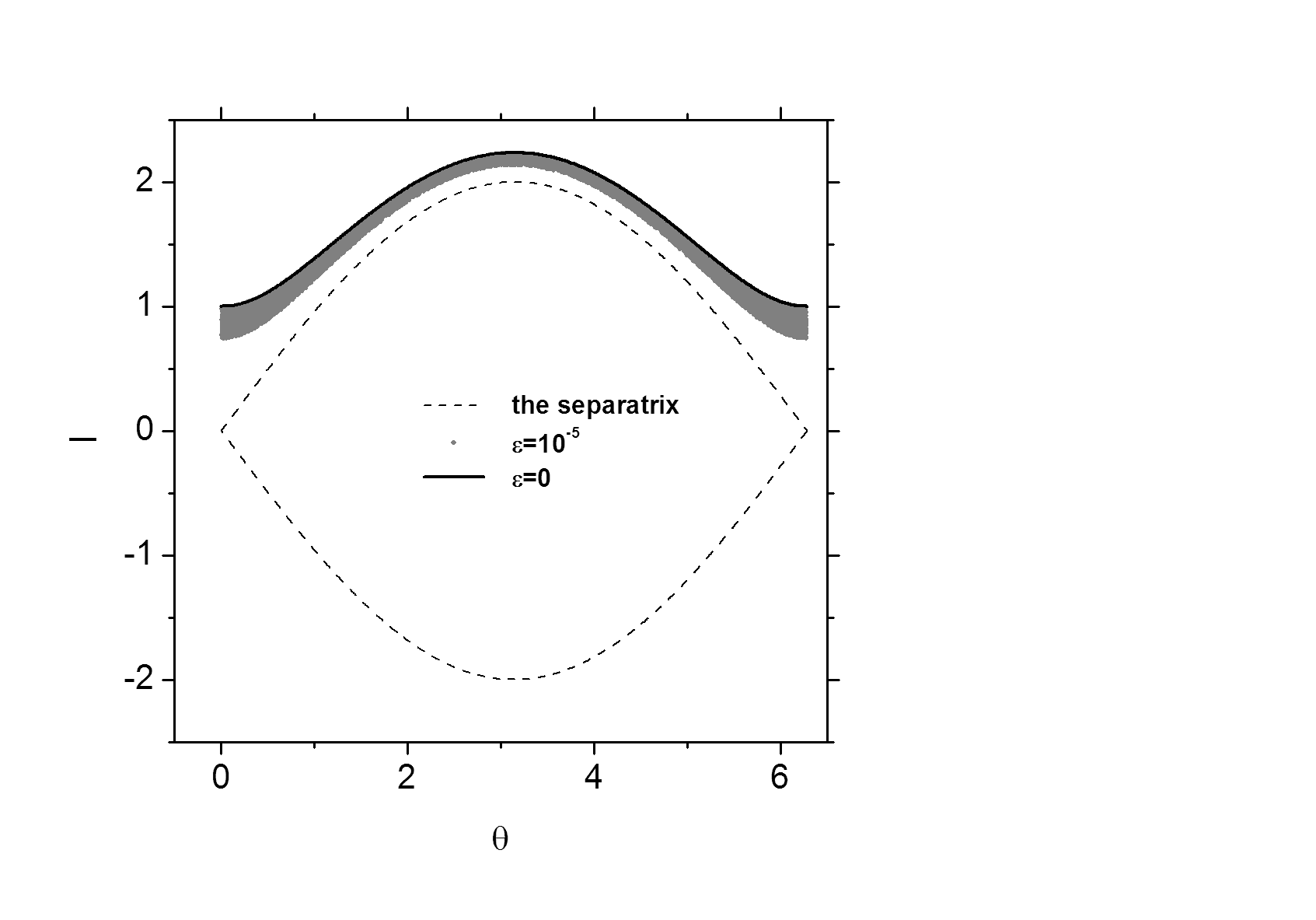
Figure 1: Phase trajectory of the dissipated solution specified by (18), (19) and (20). Also shown is the phase orbit of the unperturbed pendulum system, namely (18) with $\varepsilon=0$, which passes through the initial phase point of the dissipated solution. The dashed line depicts the spepratrix of the unperturbed pendulum.

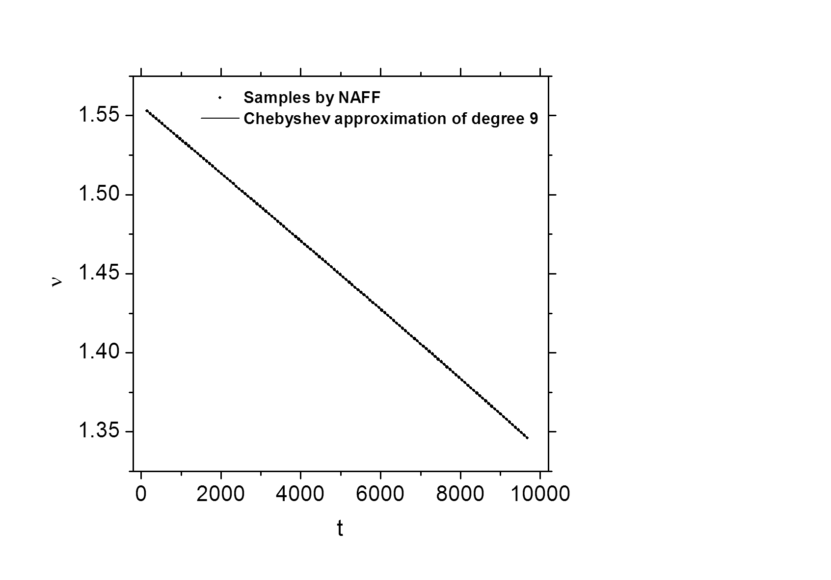
Figure 2: The changing fundamental frequency $\nu(t)$ of the dissipated solution specified by (18), (19) and (20). Also shown is a Chebyshev approximation of $\nu(t)$.

4.1 An example of dissipated solution

Consider the following weakly dissipated system

$$\frac{d^{2}\theta}{dt^{2}}=\sin(\theta)-\varepsilon\frac{d\theta}{dt}$$ (18)

where

$$\varepsilon=10^{-5}.$$ (19)

If we nullify the dissipative term $-\varepsilon\frac{d\theta}{dt}$ in (18), the system is a simple pendulum with Hamiltonian $H_{0}(I)=\frac{I^{2}}{2}+\cos(\theta)$, where $I=\dot{\theta}$. Take as an example the solution $z(t)\equiv I(t){\rm e}^{{\rm i}\ \theta(t)}$ of (18) with the following initial conditions

$$t_{0}=0,\theta_{0}=0,I_{0}=1.$$ (20)

Due to the presence of the dissipative perturbation, the phase orbit starting from $(\theta_{0},I_{0})$ decays gradually away from the unperturbed orbit passing through the same phase point. This dissipation effect is significant in the long run, as is shown in Fig.1.

As a solution of a system of 1 degree of freedom with a dissipative perturbation, the decaying $z(t)$ has a changing fundamental frequency $\nu$, which inherits the characteristic frequency of the unperturbed system and varies as the solution decays.

By numerical integration, an ephemeris of $z(t)$ is obtained at $\{t_{i}=ih:i=0,...,65535,h=0.15\}$. We then apply NAFF to 129 evenly spaced time subintervals with length $d=2046h$ and midpoints $\{\tau_{\lambda}=\frac{d}{2}+496(\lambda-1)h\}_{\lambda=1}^{129}$, respectively, to obtain a sample set of the changing frequency, $\{\tau_{\lambda},\nu(\tau_{\lambda})\}_{\lambda=1}^{129}$. This frequency sample set is shown in Fig.2. Also shown is a Chebyshev expansion approximating $\nu(t)$. This expansion is of degree $9$ and expressed as

$$\nu(t)\approx\sum_{m=0}^{9}c_{m}T_{m}(x),$$ (21)

where the Chebyshev polynomials $T_{m}(x)$ are given in (39), and $x(t)=\frac{2(t-\tau_{1})}{\tau_{129}-\tau_{1}}-1$ is the time after being normalized from $[\tau_{1},\tau_{129}]$ to the $[-1,1]$ interval on which the Chebyshev polynomials are defined. The values of the coefficients $\{c_{m}\}_{m=0}^{9}$ are listed in Table LABEL:tab_D_FFdata. We write the Chebyshev expansion approximating the phase increment, from the value at $x=0$ (i.e. $t=\frac{\tau_{1}+\tau_{129}}{2}$), associated with $\nu$ in two parts

$$\begin{array}[]{ll}\int_{(\tau_{1}+\tau_{129})/2}^{t}\mathbf{\nu}(\tau)d\tau&=\frac{\tau_{129}-\tau_{1}}{2}\int_{0}^{x(t)}\sum_{m=0}^{9}c_{m}T_{m}(x)dx\\[14.22636pt] &=\varphi_{0}T_{0}(x)+\varphi(x).\end{array}$$ (22)

In this equation, the time scaling factor $\frac{\tau_{129}-\tau_{1}}{2}$ accounts for the change of integration variable from the physical time to the normalised time, $\varphi_{0}=-\frac{\tau_{129}-\tau_{1}}{2}\varphi(0)$ is a real constant, and

$$\varphi(x)=\frac{\tau_{129}-\tau_{1}}{2}\sum_{m=1}^{10}C_{m}T_{m}(x)$$ (23)

gathers all Chebyshev polynomials of degree larger than 0 with

$$C_{m}=\left\{\begin{array}[]{l}\frac{2c_{0}-c_{2}}{2}\hskip 36.98866pt(m=1),\\ \frac{c_{m-1}-c_{m+1}}{2m}\hskip 28.45274pt(m=2,\ldots,10).\end{array}\right.$$ (24)

where $c_{10}=c_{11}=0$.

Table 2: The coefficients of the Chebyshev expansion $\sum_{m=0}^{9}c_{m}T_{m}(x(t))$ approximating $\nu(t)$, the changing fundamental frequency of the dissipated solution specified by (18), (19) and (20).

$m$	$c_{m}$
0	$+1.450265\times 10^{0}$
1	$-1.032502\times 10^{-1}$
2	$-7.924442\times 10^{-4}$
3	$-1.163806\times 10^{-4}$
4	$-7.914948\times 10^{-6}$
5	$-6.369786\times 10^{-7}$
6	$-5.975314\times 10^{-8}$
7	$-3.609371\times 10^{-9}$
8	$+1.771340\times 10^{-9}$
9	$+8.159405\times 10^{-9}$

Table 3: The leading 10 terms of (25), a representation of the dissipated solution $z(t)$ specified by (18), (19) and (20), which is obtained with $\{M,K,L,\delta_{r}\}=\{9,10,9,10^{-5}\}$

.

j	$l(j)$	$k(j)$	$Arg(a_{j})$	$|a_{j}|$
1	0	1	$-1.431544$	$1.378074489$
2	0	2	$0.278103$	$0.622837454$
3	0	3	$1.987348$	$0.159698128$
4	1	1	$1.748566$	$0.116187680$
5	0	4	$-2.587002$	$0.032622276$
6	0	-1	$-1.709654$	$0.017747854$
7	1	2	$0.133848$	$0.028210547$
8	1	3	$1.931736$	$0.027791194$
9	0	5	$-0.878547$	$0.005904572$
10	1	4	$-2.628911$	$0.009823726$

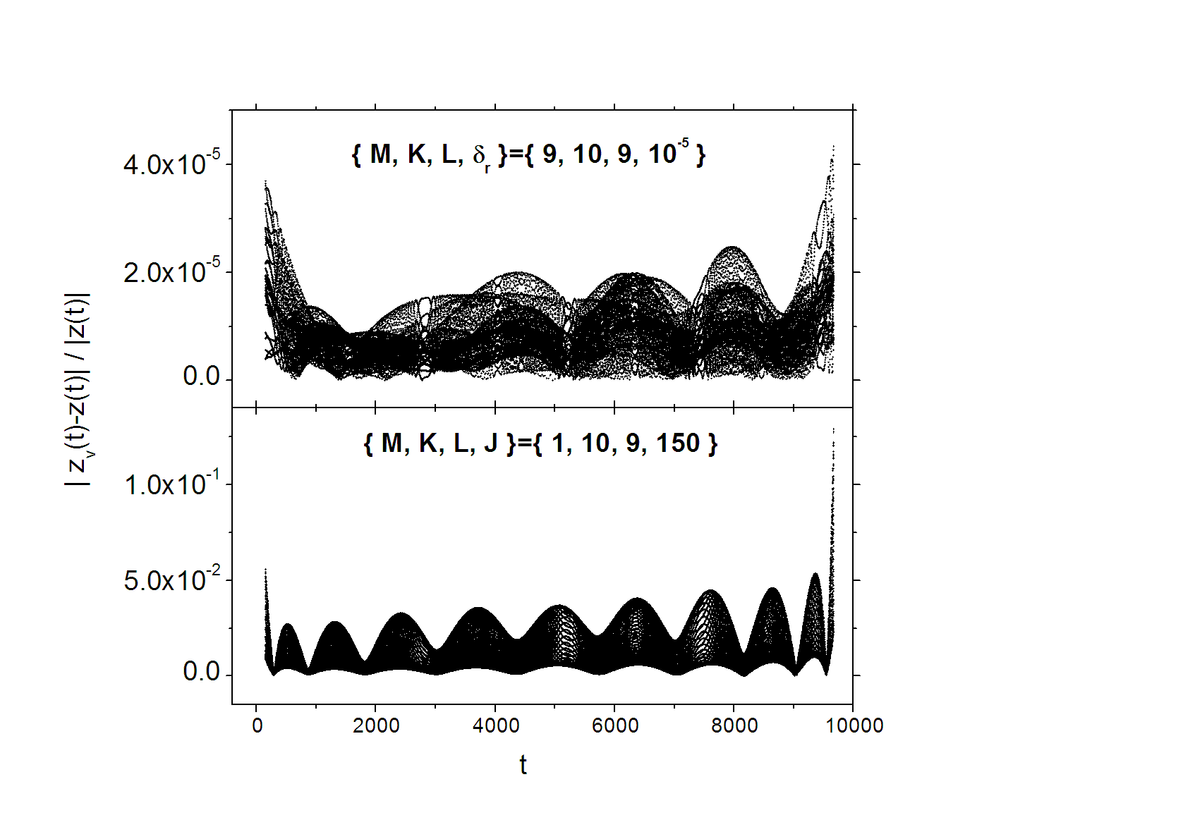
Figure 3: Errors of two different representations of the dissipated solution specified by (18), (19) and (20). In the case of the upper panel, our representation procedure is terminated with a 37-term representation, because this representation reaches the precision requirement $\delta_{r}=10^{-5}$. In the case of the lower panel, with sligtly larger error in the frequency approximation, the representation is about 4 orders less precise, though the number of representation terms is increased to 150.

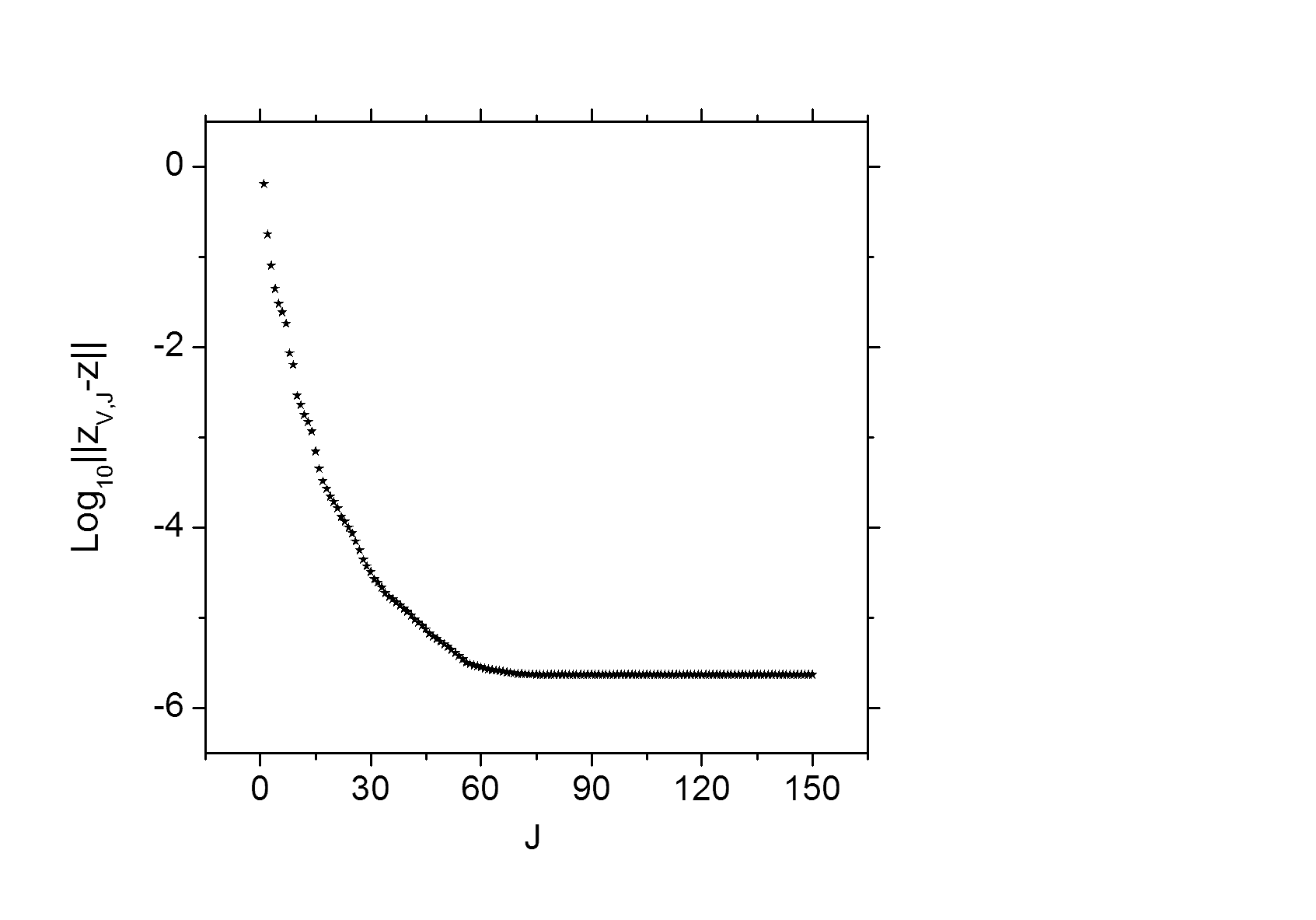
Figure 4: Convergence property of the procedure of representing the dissipated solution specified by (18), (19) and (20). The residual of representation is plotted against the number $J$ of representation terms, where other procedure parameters are fixed as $\{M,K,L\}=\{9,10,9\}$.

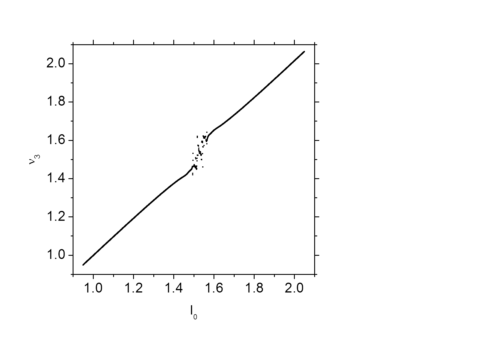
Figure 5: Fundamental frequency map of the system specified by (26) and (27). In the chaotic zone formed by resonance overlap lies the phase point $(\theta_{0},I_{0})=(0,1.535)$, which will be chosen as the initial phase point of the considered chaotic solution.

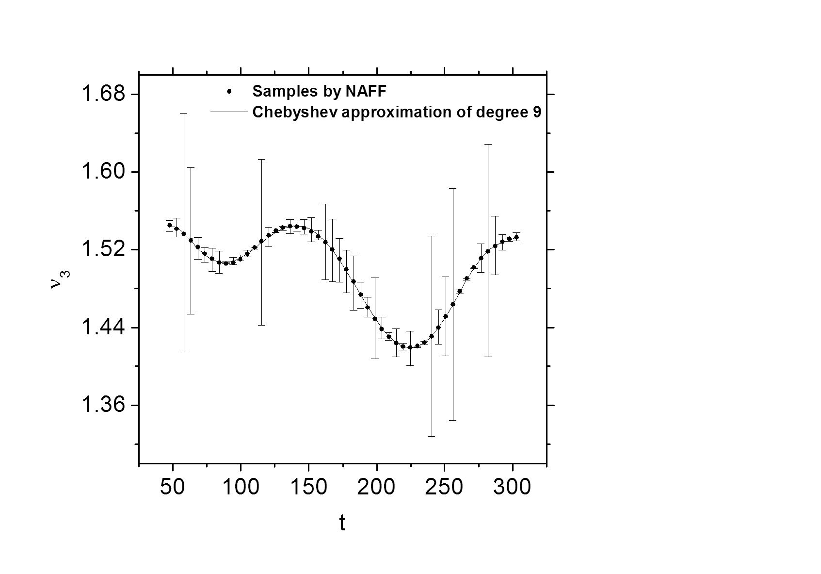
Figure 6: The changing fundamental frequency $\nu_{3}(t)$ of the chaotic solution specified by (26), (27) and (28). The samples of this frequency is computed by applying NAFF algorithm over a sliding time interval, and the errors are estimated as their respective differences from the frequencies of the quasiperiodic approximation of the solution over the same sliding time interval. Also shown is a Chebyshev appoximation of $\nu_{3}(t)$.

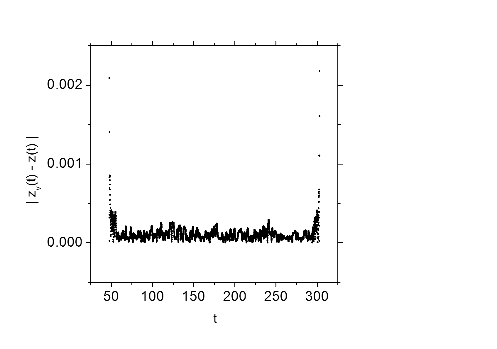
Figure 7: Error of a 100-term representation of the chaotic solution specified by (26), (27) and (28). This representation is obtained with $\{M_{1},M_{2},M_{3},K_{1},K_{2},K_{3},L_{\mathbf{k}},J\}=\{0,0,9,10,10,10,9,100\}$.

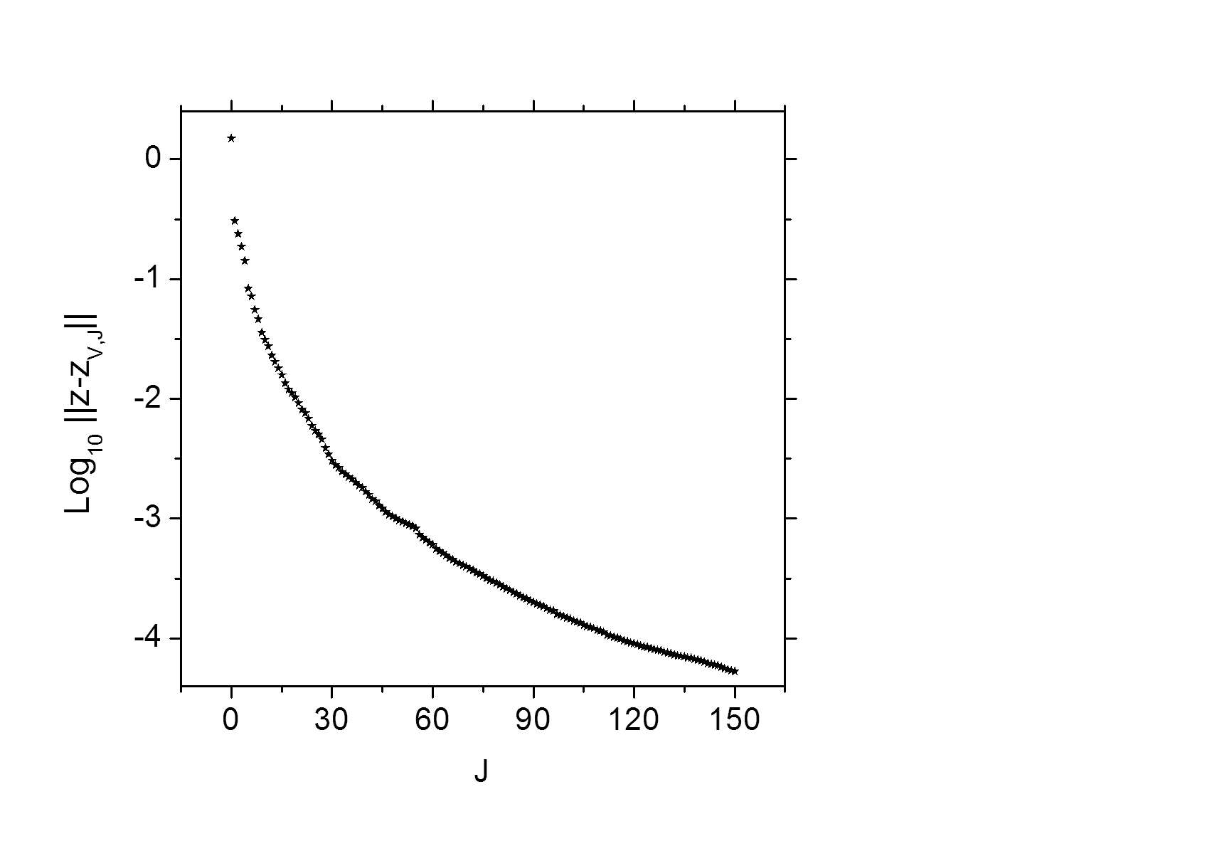
Figure 8: The convergence property of the procedure of representing the chaotic solution specified by (26), (27) and (28). The residual of representation is plotted against the number $J$ of representation terms. The other procedure parameters are fixed as $\{M_{1},M_{2},M_{3},K_{1},K_{2},K_{3},L_{\mathbf{k}}\}=\{0,0,9,10,10,10,9\}$.

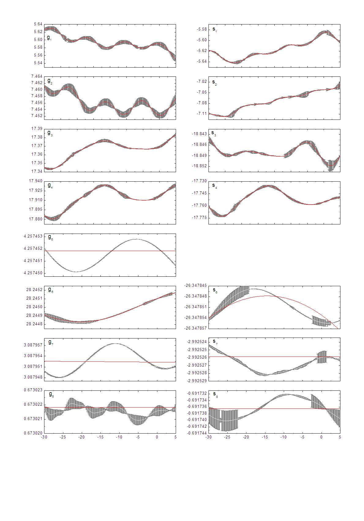
Figure 9: Variations of major fundamental frequencies of the solar system over the time interval from -35 Myr to 5 Myr with origin at J2000. These frequencies (in arcsec yr^-1) are computed by applying the NAFF algorithm to the proper modes of the secular solar system associated respectively with major planets. The errors in the resulting frequency samples are estimated as the difference between the frequencies computed respectively from the original ephemeris and its quasiperiodic approximation. Also shown in this figure are the Chebyshev approximations of these varing fundamental frequencies (red curves), which are specified in Table 4.

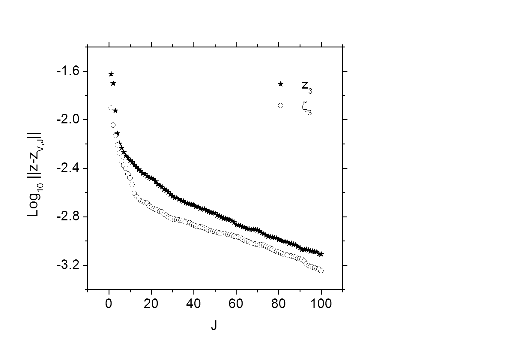
Figure 10: Convergence property of the two representation procedures leading respectively to the 100-term representations of $z_{3}(t)$ and $\zeta_{3}(t)$. The residual of representation is plotted against the number $J$ of representation terms.

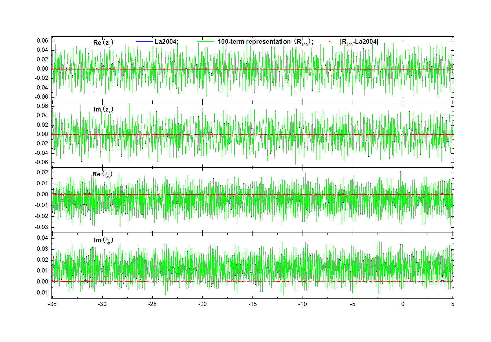
Figure 11: Comparison between the eccentricity and inclination ephemerides of La2004 and their respective 100-term representations over the time interval from -35 Myr to 5 Myr with origin at J2000. Both representions are in the form of (31), with the Chebyshev expansions approximating the fundamental frequencies specified in Table 4, and main frequency index vectors and complex amplitudes of all 100 terms in the on-line electronic files under names z3R100.dat and zeta3R100.dat, respectively.

Figure 12: Comparison between the eccentricity ephemeris $z_{3}$ and the inclination ephemeris $\zeta_{3}$ of La2004 and their respective representations by NAFF ($\Re_{NAFF}$) and by the present algorithms ($\Re$). The number of terms of $z_{3}$-representation is 50 for both $\Re_{NAFF}$ and $\Re$, and the number is 41 in the case of $\zeta_{3}$.

Table 4: The coefficients of Chebyshev expansion $\sum_{m}c_{m}T_{m}$ approximating the major fundamental frequencies $(g_{1},...,g_{8},s_{1},..,s_{8})$ (arcsec yr^-1) of the solar system over the time interval from -35 Myr to 5 Myr with origin at J2000. Also listed are the used constant libration frequencies $r_{1}$ and $r_{2}$ (arcsec yr^-1).

	$m$	$c_{m}$		$m$	$c_{m}$
$g_{1}$	$0$	$5.59436858$	$s_{1}$	$0$	$-5.61412432$
	$1$	$-0.02916946$		$1$	$0.01897975$
	$2$	$0.00259949$		$2$	$0.00616405$
	$3$	$-0.00858191$		$3$	$-0.00967633$
	$4$	$-0.00538351$		$4$	$-0.00048289$
	$5$	$-0.00216691$		$5$	$-0.00405450$
	$6$	$-0.00311006$		$6$	$-0.00319098$
	$7$	$0.00137912$		$7$	$0.00116236$
	$8$	$-0.00225709$		$8$	$-0.00048593$
	$9$	$0.00318074$		$9$	$0.00207233$
	$10$	$0.00431717$		$10$	$0.00194425$
	$11$	$-0.00288184$		$11$	$-0.00103824$
	$12$	$-0.00189708$		$12$	$-0.00117501$
	$13$	$0.00127879$		$13$	$0.00006311$
	$14$	$0.00065723$		$14$	$0.00030964$
	$15$	$-0.00017362$		$15$	$-0.00037496$
$g_{2}$	$0$	$7.45660678$	$s_{2}$	$0$	$-7.07313208$
	$1$	$-0.00276205$		$1$	$0.04218433$
	$2$	$0.00177713$		$2$	$-0.00001315$
	$3$	$0.00056064$		$3$	$-0.00225169$
	$4$	$-0.00002096$		$4$	$0.00386256$
	$5$	$0.00090782$		$5$	$-0.00280878$
	$6$	$0.00096229$		$6$	$0.00247914$
	$7$	$-0.00024908$		$7$	$0.00109449$
	$8$	$0.00042855$		$8$	$-0.00064733$
	$9$	$-0.00071228$		$9$	$0.00229722$
	$10$	$-0.00091971$		$10$	$-0.00000725$
	$11$	$0.00061668$		$11$	$-0.00193901$
	$12$	$0.00047006$		$12$	$0.00088350$
	$13$	$-0.00024111$		$13$	$0.00053257$
	$14$	$-0.00015053$		$14$	$0.00024897$
	$15$	$0.00007778$		$15$	$0.00024128$
$g_{3}$	$0$	$17.36445990$	$s_{3}$	$0$	$-18.84810087$
	$1$	$0.01585020$		$1$	$-0.00165582$
	$2$	$-0.00496995$		$2$	$0.00007105$
	$3$	$0.00540088$		$3$	$-0.00140634$
	$4$	$0.00496032$		$4$	$0.00050744$
	$5$	$-0.00226103$		$5$	$0.00039039$
	$6$	$-0.00004476$		$6$	$0.00135948$
	$7$	$0.00006943$		$7$	$0.00065306$
	$8$	$0.00007190$		$8$	$-0.00041702$
	$9$	$-0.00037475$		$9$	$-0.00026792$
	$10$	$-0.00059252$		$10$	$-0.00018687$
	$11$	$0.00025574$		$11$	$0.00004492$
	$12$	$0.00035119$		$12$	$0.00013288$
	$13$	$-0.00020600$		$13$	$0.00001794$
	$14$	$-0.00000042$		$14$	$-0.00005746$
	$15$	$0.00011279$
$g_{4}$	$0$	$17.91086281$	$s_{4}$	$0$	$-17.75496646$
	$1$	$0.02044603$		$1$	$0.00670633$
	$2$	$-0.00851446$		$2$	$-0.00717162$
	$3$	$0.00812180$		$3$	$0.00313019$
	$4$	$0.00866961$		$4$	$0.00807398$
	$5$	$-0.00482118$		$5$	$-0.00498282$
	$6$	$-0.00137335$		$6$	$-0.00116638$
	$7$	$0.00011721$		$7$	$0.00058378$
	$8$	$0.00083465$		$8$	$0.00021726$
	$9$	$-0.00041179$		$9$	$0.00016650$
	$10$	$-0.00109334$		$10$	$-0.00060643$
	$11$	$0.00069484$		$11$	$0.00014173$
	$12$	$0.00045529$		$12$	$0.00039520$
	$13$	$-0.00029042$		$13$	$-0.00024600$
	$14$	$-0.00014170$		$14$	$-0.00006598$
	$15$	$0.00008189$		$15$	$0.00012665$
$g_{5}$	$0$	$4.25745185$	$s_{5}$	$0$	$0.00000015$
$g_{6}$	$0$	$28.24498422$	$s_{6}$	$0$	$-26.34785292$
	$1$	$0.00010582$		$1$	$0.00000053$
	$2$	$0.00011695$		$2$	$-0.00000514$
	$3$	$-0.00002698$
	$4$	$-0.00001157$
$g_{7}$	$0$	$3.08795246$	$s_{7}$	$0$	$-2.99252583$
	$1$	$-0.00000017$
$g_{8}$	$0$	$0.67302182$	$s_{8}$	$0$	$-0.69173649$
				$1$	$0.00000001$
$r_{1}$	$0$	$0.251085\ \ \ \$	$r_{2}$	$0$	$0.117222\ \ \ \$

Table 5: The leading 40 terms of the 100-term representation $z_{3}(t)$, as expressed in (31).

No.	$\langle\mathbf{k},\mathbf{f}\rangle$	$\mathrm{Abs}(a_{\mathbf{k}})\times 10^{6}$	$\mathrm{Arg}(a_{\mathbf{k}})$ (degree)
1	$g_{5}$	$18984$	$-68.812$
2	$g_{2}$	$16088$	$95.535$
3	$g_{4}$	$13041$	$17.345$
4	$g_{3}$	$9042$	$-54.984$
5	$g_{1}$	$4314$	$-175.273$
6	$g_{4}-r_{1}$	$2583$	$-92.093$
7	$g_{3}-r_{1}$	$2415$	$15.391$
8	$g_{3}+r_{1}+r_{2}$	$2377$	$-136.939$
9	$g_{4}+s_{3}-s_{4}$	$1934$	$-128.504$
10	$g_{6}$	$1498$	$160.676$
11	$2g_{1}-g_{5}$	$1393$	$82.417$
12	$g_{3}+g_{4}-g_{6}$	$1372$	$178.968$
13	$g_{1}-r_{2}$	$1298$	$140.905$
14	$g_{3}-s_{3}+s_{4}$	$1282$	$-87.475$
15	$g_{2}-r_{2}$	$1156$	$-127.879$
16	$g_{4}-2r_{1}$	$1153$	$15.739$
17	$g_{1}+r_{2}$	$1085$	$49.430$
18	$g_{2}-g_{3}+g_{6}-r_{2}$	$1028$	$-40.633$
19	$g_{4}-r_{2}$	$946$	$149.088$
20	$g_{2}+r_{2}$	$942$	$123.828$
21	$-g_{1}+2g_{4}-g_{5}+s_{3}$	$916$	$82.353$
22	$-g_{3}+2g_{4}-2r_{1}$	$903$	$63.075$
23	$g_{3}+s_{3}-s_{4}$	$824$	$150.057$
24	$g_{3}+2r_{1}$	$816$	$145.441$
25	$g_{4}+r_{1}$	$806$	$165.483$
26	$g_{4}+s_{3}-s_{4}-r_{1}$	$756$	$113.428$
27	$g_{1}-s_{3}+s_{4}+r_{2}$	$712$	$-121.353$
28	$g_{4}-s_{3}+s_{4}$	$697$	$-14.943$
29	$2g_{3}-g_{4}+2r_{2}$	$605$	$-21.586$
30	$g_{7}$	$577$	$-146.073$
31	$g_{4}+r_{2}$	$573$	$52.634$
32	$g_{3}+r_{2}$	$504$	$-21.947$
33	$g_{1}+g_{5}-g_{7}+r_{1}$	$432$	$152.449$
34	$-g_{1}+g_{2}+g_{5}-r_{2}$	$383$	$-28.070$
35	$g_{3}+r_{1}$	$275$	$-4.253$
36	$g_{3}-r_{2}$	$144$	$89.319$
37	$g_{2}-r_{1}-r_{2}$	$121$	$-36.562$
38	$g_{2}-r_{1}+r_{2}$	$104$	$-105.175$
39	$-g_{1}+g_{4}+g_{5}$	$92$	$-173.117$
40	$g_{1}-r_{1}$	$87$	$99.123$

Table 6: The leading 40 terms of the 100-term representation $\zeta_{3}(t)$, as expressed in (31).

No.	$\langle\mathbf{k},\mathbf{f}\rangle$	$\mathrm{Abs}(b_{\mathbf{k}})\times 10^{6}$	$\mathrm{Arg}(b_{\mathbf{k}})$ (degree)
1	$s_{5}$	$13774$	$107.587$
2	$s_{3}$	$8666$	$-62.318$
3	$s_{4}$	$4647$	$96.756$
4	$s_{1}$	$4085$	$27.817$
5	$s_{2}$	$3312$	$80.364$
6	$g_{3}-g_{4}+s_{4}$	$2745$	$-167.132$
7	$s_{2}+2r_{2}$	$2041$	$-44.496$
8	$s_{2}+r_{2}$	$1543$	$125.410$
9	$g_{3}-g_{4}+s_{3}$	$1530$	$-137.669$
10	$s_{1}+s_{3}-s_{4}-r_{2}$	$1469$	$91.798$
11	$s_{2}-r_{2}$	$1450$	$23.071$
12	$s_{1}+r_{2}$	$1417$	$-116.942$
13	$s_{6}$	$1333$	$110.029$
14	$s_{7}$	$889$	$9.186$
15	$s_{2}+r_{1}$	$646$	$-50.277$
16	$s_{8}$	$641$	$26.053$
17	$s_{3}-r_{1}$	$613$	$-178.905$
18	$s_{1}+s_{3}-s_{4}$	$532$	$-177.568$
19	$s_{1}-2r_{2}$	$518$	$101.955$
20	$s_{3}-r_{2}$	$484$	$106.762$
21	$g_{3}-g_{4}+s_{3}+r_{1}$	$481$	$-21.125$
22	$g_{3}-g_{4}+s_{2}+r_{1}$	$445$	$-5.831$
23	$s_{2}-s_{3}+s_{4}$	$364$	$72.700$
24	$s_{2}-s_{3}+s_{4}-r_{2}$	$344$	$31.282$
25	$s_{2}-r_{1}$	$341$	$20.734$
26	$s_{2}-2r_{2}$	$320$	$-51.578$
27	$g_{3}-g_{4}+s_{1}$	$315$	$-118.127$
28	$g_{3}-s_{1}+s_{6}+s_{7}-s_{8}$	$304$	$172.667$
29	$s_{1}-r_{1}$	$293$	$149.314$
30	$-s_{4}+s_{6}-s_{7}+2s_{8}$	$293$	$-76.858$
31	$s_{1}+2r_{1}-r_{2}$	$292$	$134.167$
32	$-g_{3}+s_{5}+s_{8}+r_{1}$	$285$	$-170.886$
33	$-g_{3}+g_{4}+s_{2}$	$268$	$47.758$
34	$-g_{3}+g_{4}+s_{2}-r_{2}$	$258$	$-27.836$
35	$-g_{3}+g_{4}+s_{4}$	$244$	$-18.592$
36	$g_{4}+s_{6}-s_{8}+r_{1}$	$230$	$109.121$
37	$g_{3}-g_{4}+s_{4}-r_{1}$	$221$	$-91.732$
38	$s_{2}+s_{5}-s_{8}-2r_{1}$	$217$	$173.446$
39	$-g_{3}+g_{4}+s_{2}-r_{1}$	$198$	$24.257$
40	$s_{1}+2r_{1}$	$78$	$77.412$

This completes the determination of $\varphi(x)$, which will be used in the following. With the procedure parameters $\{M,K,L,\delta_{r}\}=\{9,10,9,10^{-5}\}$, we obtain a 37-term representation

$$z_{37}(t)=\sum_{j=1}^{37}a_{j}T_{l(j)}(x){\rm e}^{{\rm i}\varphi_{k(j)}(x)}\ \ \mathrm{with}\ \ x=\frac{2(t-\tau_{1})}{\tau_{129}-\tau_{1}}-1$$ (25)

of the solution $z(t)$, where $T_{l(j)}(x)$ is the Chebyshev polynomial of degree $l(j)$, and $\varphi_{k(j)}(x)=k(j)\varphi(x)$ the phase increment associated with the frequency $k(j)\nu$. The data needed for specifying the first 10 representation terms are given in Table LABEL:tab_D_termdata.

Now, we discuss how the procedure parameters affect the precision of the resulting representation. For this, let’s first consider a 150-term representation obtained by resetting $M=1$. This resetting introduces only a small discrepancy in $\nu(t)$, since $|c_{m}/c_{0}|<6\times 10^{-4}$ for $m>1$. But the precision of this representation is several orders less precise than the previous one, as seen by comparing the two panels of Fig.3. This is because the whole considered time interval is long, and so, the small discrepancy in $\nu(t)$ can result in significant phase errors. On the other hand, however, the fact that there is no terms with either $|k|>8$ or $l>4$ in the 37-term representation indicates that the representation model practically converges with respect to $K$ and $L$. Our representation procedure also converges rapidly with respect to $J$. This is illustrated in Fig.4, for which the procedure parameters excluding $J$ are fixed as $\{M,K,L\}=\{9,10,9\}$.

4.2 An example of chaotic solutions of Hamiltonian system

Consider the following Hamiltonian system,

$$H(I,\theta,t)=\frac{I^{2}}{2}+\varepsilon\cos(\theta)[1+\cos(\nu_{1}t)+\cos(\nu_{2}t)],$$ (26)

where

$$\varepsilon=5\times 10^{-3},\nu_{1}=1.5,\nu_{2}=\frac{\pi}{2}.$$ (27)

A solution of this system has three fundamental frequencies. The first two are simply the forcing frequencies $\nu_{1}$ and $\nu_{2}$, which are non-commensurable. The other, denoted as $\nu_{3}$, can be approximated in the similar way as in the previous subsection.

By the analysis of the frequency map (e.g. Laskar, 1999), defined as $I_{0}\rightarrow\nu_{3}$ with $\theta_{0}=0$ and shown in Fig.5, we know that the phase point

$$t_{0}=0,\theta_{0}=0,I_{0}=1.535,$$ (28)

lies in a chaotic zone formed by resonance overlap. And the solution $z(t)$ starting from this point is chaotic.

An ephemeris of $z(t)$ is obtained by the symplectic integrator SBABc4 (Laskar & Robutel, 2001) at $\{t_{i}=ih:i=0,...,4095,h=0.186058\}$. We then apply NAFF to 129 evenly spaced time intervals with length $d=512h$ and midpoints $\{\tau_{\lambda}=\frac{d}{2}+28(\lambda-1)h\}_{\lambda=1}^{129}$, respectively. This gives the sample set $\{\tau_{\lambda},\nu_{3,\lambda}\}_{\lambda=1}^{129}$, partly shown in Fig.6 together with a Chebyshev approximation. It should be noted that there are two intrinsically different error sources in the present way of approximating a changing frequency. One is related to the NAFF process that gives the samples of the frequency, while the other related to the fitting process that leads to a Chebyshev approximation of the frequency. Accordingly, we consider the Chebyshev approximation as sufficiently good if it deviates from the frequency sample set much less than the sample uncertainties. As shown in Fig.6, this requirement can be met with the Chebyshev polynomial of degree $M_{3}=9$.

Test calculations show that our representation procedure cannot lead to an acceptable representation of the solution on the whole sampling time interval. There are two possible reasons for this.

The most intrinsic reason would be that our solution experiences passages into or out of resonance zones. Such a passage is associated with a shift between circulation and libration of the corresponding resonance angle, and so, with occurrence or disappearance of certain terms. If some of these terms are significant enough in the whole considered time interval $(\tau_{1},\tau_{129})$, then there would be no way to get any acceptable non-piecewise representation. Therefore, we will restrict ourselves to the shorter time interval $(\tau_{1},\tau_{50})$.

Another possible reason is that there is one or more significant libration frequencies, which are not taken into consideration when we generate the function basis $B$. While it is easy to make a necessary extension of $B$ in order to include known libration frequencies (see section 5), it is not that straightforward to identify and sample these frequencies (Laskar, 1990). To show the flexibility of our algorithm, we will not search for any libration frequency and make the corresponding extension of $B$. The flexibility comes from the fact that, if we choose reasonably large values of our procedure parameters $K_{n}$’s, then the resulting set of frequencies would be dense enough over a large frequency interval, in the sense that every important libration frequency is not far from at least one element of the frequency set.

Setting the procedure parameters as

$$\{M_{1},M_{2},M_{3},K_{1},K_{2},K_{3},L_{\mathbf{k}},J\}=\{0,0,9,10,10,10,9,100\},$$

we obtain a 100-term representation of our solution. Fig.7 shows that the errors of this representation are typically of order less than $10^{-4}I_{0}$. And, Fig.8 illustrates, in the same way as in the previous subsection, the convergence property of the representation procedure.

5 Application to planetary ephemerides

Numerical integration is now an efficient way of constructing ephemerides of the solar system bodies with high precision. For practical applications, however, it can be useful to represent analytically, and thus in a continuous way, these discrete solutions.

These representations can be done in the form of segmented Chebyshev expansions, like the ones representing the classical planetary ephemerides as INPOP (e.g. Fienga et al., 2008), or other generally applied approximation models without physical basis. A drawback of these representations is that they require large amount of data. In order to get compact representations, Chapront (1995) uses a model of Poisson series, with fixed main frequencies, that were obtained with the NAFF algorithm. Though this model already involves some long-term or long-period-term effects by allowing Poisson terms, and as thus, works well with planetary ephemerides of five outer planets over a few hundred years, it does not take into consideration the frequency drifts, and cannot be used over million of years.

The frequency drifts are important over a few tens of million years, as shown by Laskar (1990). The algorithm developed in the present paper should thus be more appropriate in representing ephemerides spanning this long time interval. It is thus interesting to test whether the present algorithm can be used to represent over such a time scale the long-term numerical solution of major solar system bodies, (e.g. Laskar et al., 2004). For this, we apply our algorithm to the eccentricity and inclination variables of the Earth, i.e.,

$$z_{3}=e_{3}\exp(i\varpi_{3})\ \ \mathrm{and}\ \ \zeta_{3}=\sin(i_{3}/2)\exp(i\Omega_{3}).$$ (29)

To be more precise, $e_{3}\ \mathrm{and}\ i_{3}$ are the eccentricity and inclination, respectively, of the instantaneous orbit of the Earth-Moon barycenter, and $\varpi_{3}\ \mathrm{and}\ \Omega_{3}$ are, respectively, the longitudes of the perihelion and of the node of the same orbit with respect to the fixed J2000.0 equatorial reference system.

The chaotic behaviour of the terrestrial orbit certainly limit the time span over which this orbit can be precisely determined, but $z_{3}$ and $\zeta_{3}$ from La2004 are reliable and precise at least over the time span $[-35\mathrm{Myr},+5\mathrm{Myr}]$ (Laskar et al., 2011). Therefore, we restrict our representations to this time span. Test calculations show that our algorithm can lead to compact and precise representations for both degrees of freedom. With different procedure parameters, the resulting representations contain very different terms. This confirms the flexibility of the present algorithm.

In order to give representations as physical as possible, we will resort to the knowledge we have for the solution. Following Laskar et al. (2004), we compute the fundamental frequencies of the secular solar system by applying the NAFF algorithm over time intervals of length 20 Myr for the proper modes $(z^{\bullet}_{1},...,z^{\bullet}_{4},\zeta^{\bullet}_{1},...,\zeta^{\bullet}_{4})$, and 50 Myr for the proper modes $(z^{\bullet}_{5},...,z^{\bullet}_{8},\zeta^{\bullet}_{5},...,\zeta^{\bullet}_{8})$, respectively. From -35 Myr to 5 Myr with step 0.1 Myr, we generate the samples of the fundamental frequencies $(g_{1},...,g_{8},s_{1},...,s_{8})$ corresponding to these proper modes. The resulting nominal value of $s_{5}$ is about $0.00000015\ \mathrm{arcsec\ yr}^{-1}$. The other frequency samples are shown respectively in the panels of Fig.9, where the errors are estimated as the difference between the values of a frequency computed from the associated ephemeris and its quasiperiodic approximation. Also shown in this figure are the Chebyshev approximations of these fundamental frequencies. All of these Chebyshev approximations, the coefficients of which are listed in Table 4, are obtained respectively by truncating the ones of degree 15. The truncation criterion is roughly that the discrepancy in a fundamental frequency should not induce an error in phase larger than $2\pi/10^{4}$ over several tens of million years.

There are two important libration frequencies, i.e. $r_{1}=0.251085\ \mathrm{arcsec\ yr}^{-1}$ of the resonance argument $2(\varpi^{\bullet}_{4}-\varpi^{\bullet}_{3})-(\Omega^{\bullet}_{4}-\Omega^{\bullet}_{3})$ and $r_{2}=0.117222\ \mathrm{arcsec\ yr}^{-1}$ of $2(\varpi^{\bullet}_{1}-\varpi^{\bullet}_{5})-(\Omega^{\bullet}_{1}-\Omega^{\bullet}_{2})$. To include them as additional fundamental frequencies, we express a main frequency as

$$\omega=\sum_{i=1}^{8}(m_{i}g_{i}+n_{i}s_{i})+\sum_{j=1}^{2}k_{j}r_{j},$$ (30)

The d’Alembert characteristic, i.e. $\sum_{i=1}^{8}(m_{i}+n_{i})=1$, will be used to exclude non-physical frequency index vectors.

To show to what degree our algorithm is practically useful, we discuss here the following two 100-term representations ($\Re_{100}$ for short),

$$z_{3}(t)=\sum_{j=1}^{100}a_{\mathbf{k}(j)}{\rm e}^{{\rm i}\varphi_{\mathbf{k}(j)}(t)},\ \ \zeta_{3}(t)=\sum_{j=1}^{100}b_{\mathbf{k}(j)}{\rm e}^{{\rm i}\varphi_{\mathbf{k}(j)}(t)},$$ (31)

where, with $\mathbf{f}=(g_{1},...,g_{8},s_{1},...,s_{8},r_{1},r_{2})$ and $\mathbf{k}=(m_{1},...,m_{8},n_{1},...,n_{8},k_{1},k_{2})$, the phase increment $\varphi_{\mathbf{k}}(t)=\int_{0}^{t}\langle\mathbf{k},\mathbf{f(\tau)}\rangle d\tau$ is associated with the main frequency $\langle\mathbf{k},\mathbf{f}\rangle$. The way the residuals decrease with the increasing number of representation terms in the two representation procedures of $\Re_{100}$ are shown in Fig.10.

The leading 40 terms of these two representations are given, respectively, in Tables 5 and 6, where the terms are reordered according to their real amplitudes and data are rounded to a convenient number of digits. Comparing these results with the ones given in tables 4 and 5 of Laskar (1990), we find that they are coherent with each other in the sense that all the main frequencies explicitly identified previously can be found in the present tables.

The on-line electronic files associated with the present paper, i.e. z3R100.dat and zeta3R100.dat, are the full version of Table 5 and Table 6, respectively. They are plain text tables providing all terms of $\Re_{100}$ in the form of (31). Together with the data presented in Table 4 for computing $\mathbf{f}$, these two tables can be used to compute the eccentricity and inclination variables from $\Re_{100}$. The errors of $\Re_{100}$ as solution representation are shown in Fig.11. From this figure, we expect that the present algorithm should be efficient in producing compact and precise representations of long-term ephemerides of major solar system bodies.

To conclude, we illustrate explicitly the advantage in the representation of ephemerides of taking into consideration the frequency drifts by comparing the representations given respectively by a direct use of NAFF and the modified present algorithms. The quasi-periodic representations ($\Re_{NAFF}$ for short) of the same $z_{3}$- and $\zeta_{3}$-ephemeris given by the standard realization of NAFF, which is a built-in tool of the algebraic system TRIP (http://www.imcce.fr/trip/), have respectively 50 and 41 terms. NAFF stops recovering more terms because it encounters a frequency that, at a given level of precision, is already recovered in a previous step. To show more precisely the advantage of taking frequency drifts into consideration, we produce for $z_{3}$ and $\zeta_{3}$, respectively, a representation ($\Re$) with the same number of terms as the corresponding $\Re_{NAFF}$ representation. The comparison between $\Re$ and $\Re_{NAFF}$ is shown in Fig.12. From this figure, we see clearly the improvements brought by introducing frequency drifts into the representation model.

Appendix A Chebyshev polynomials

Chebyshev polynomials as defined by the following recurrence relation

$$\begin{array}[]{l}T_{0}(x)=1,\ \ T_{1}(x)=x\hskip 106.69783pt(-1\leq x\leq 1)\\ T_{m+1}(x)=2xT_{m}(x)-T_{m-1}(x)\hskip 79.6678pt(m>1)\end{array}$$ (32)

form a non-normalized but orthogonal basis under the inner product

$$\langle f(x),g(x)\rangle=\int_{-1}^{1}\frac{f(x)g(x)}{\sqrt{1-x^{2}}}dx.$$ (33)

This can be easily checked by straightforward calculations

$$\langle T_{i}(x),T_{j}(x)\rangle=\int_{-1}^{1}\frac{T_{i}(x)T_{j}(x)}{\sqrt{1-x^{2}}}dx=\left\{\begin{array}[]{l}\pi\hskip 36.41948pt(i=j=0)\\ \pi/2\hskip 28.45274pt(i=j\neq 0)\\ 0\hskip 37.27303pt(i\neq j).\end{array}\right.$$ (34)

Their linear combination, called Chebyshev expansion, is often used to approximate a function $h(x)$ defined on $[-1,1]$

$$h(x)\approx h_{c}(x)=\sum_{m=0}^{M}c_{m}{T_{m}(x)},$$ (35)

where

$$c_{m}=\left\{\begin{array}[]{l}\frac{1}{\pi}\langle h(x),T_{m}(x)\rangle\hskip 36.41948pt(m=0)\\ \\ \frac{2}{\pi}\langle h(x),T_{m}(x)\rangle\hskip 36.41948pt(m\neq 0).\end{array}\right.$$ (36)

The indefinite integral of the Chebyshev expansion $h_{c}(x)$ writes, up to an arbitrary constant,

$$H_{c}(x)=\sum_{m=1}^{M+1}C_{m}{T_{m}(x)},$$ (37)

where, with $c_{M+1}=c_{M+2}=0$,

$$C_{m}=\left\{\begin{array}[]{l}\frac{2c_{0}-c_{2}}{2}\hskip 36.98866pt(m=1),\\ \frac{c_{m-1}-c_{m+1}}{2m}\hskip 28.45274pt(m=2,\ldots,M+1).\end{array}\right.$$ (38)

The explicit expressions of the Chebyshev polynomials up to degree 15 are listed below

$$\begin{array}[]{l}T_{0}(x)=1\\ T_{1}(x)=x\\ T_{2}(x)=2x^{2}-1\\ T_{3}(x)=4x^{3}-3x\\ T_{4}(x)=8x^{4}-8x^{2}+1\\ T_{5}(x)=16x^{5}-20x^{3}+5x\\ T_{6}(x)=32x^{6}-48x^{4}+18x^{2}-1\\ T_{7}(x)=64x^{7}-112x^{5}+56x^{3}-7x\\ T_{8}(x)=128x^{8}-256x^{6}+160x^{4}-32x^{2}+1\\ T_{9}(x)=256x^{9}-576x^{7}+432x^{5}-120x^{3}+9x\\ T_{10}(x)=512x^{10}-1280x^{8}+1120x^{6}-400x^{4}+50x^{2}-1\\ T_{11}(x)=1024x^{11}-2816x^{9}+2816x^{7}-1232x^{5}+220x^{3}-11x\\ T_{12}(x)=2048x^{12}-6144x^{10}+6912x^{8}-3584x^{6}+840x^{4}-72x^{2}+1\\ T_{13}(x)=4096x^{13}-13312x^{11}+16640x^{9}-9984x^{7}+2912x^{5}-364x^{3}+13x\\ T_{14}(x)=8192x^{14}-28672x^{12}+39424x^{10}-26880x^{8}+9408x^{6}-1568x^{4}+98x^{2}-1\\ T_{15}(x)=16384x^{15}-61440x^{13}+92160x^{11}-70400x^{9}+28800x^{7}-6048x^{5}+560x^{3}-15x.\end{array}$$ (39)