Attaining Capacity with Algebraic Geometry Codes through the $(U|U+V)$ Construction and Koetter-Vardy Soft Decoding

Abstract

In this paper we show how to attain the capacity of discrete symmetric channels with polynomial time decoding complexity by considering iterated $\left(U\mid U+V\right)$ constructions with Reed-Solomon code or algebraic geometry code components. These codes are decoded with a recursive computation of the a posteriori probabilities of the code symbols together with the Koetter-Vardy soft decoder used for decoding the code components in polynomial time. We show that when the number of levels of the iterated $\left(U\mid U+V\right)$ construction tends to infinity, we attain the capacity of any discrete symmetric channel in this way. This result follows from the polarization theorem together with a simple lemma explaining how the Koetter-Vardy decoder behaves for Reed-Solomon codes of rate close to $1$. However, even if this way of attaining the capacity of a symmetric channel is essentially the Arıkan polarization theorem, there are some differences with standard polar codes. Indeed, with this strategy we can operate succesfully close to channel capacity even with a small number of levels of the iterated $\left(U\mid U+V\right)$ construction and the probability of error decays quasi-exponentially with the codelength in such a case (i.e. exponentially if we forget about the logarithmic terms in the exponent). We can even improve on this result by considering the algebraic geometry codes constructed in [TVZ82]. In such a case, the probability of error decays exponentially in the codelength for any rate below the capacity of the channel. Moreover, when comparing this strategy to Reed-Solomon codes (or more generally algebraic geometry codes) decoded with the Koetter-Vardy decoding algorithm, it does not only improve the noise level that the code can tolerate, it also results in a significant complexity gain.

1 Introduction

Improving upon the error correction performance of Reed-Solomon codes.

Reed-Solomon codes are among the most extensively used error correcting codes. It has long been known how to decode them up to half the minimum distance. This gives a decoding algorithm that is able to correct a fraction $\frac{1-R}{2}$ of errors in a Reed-Solomon code of rate $R$. However, it is only in the late nineties that a breakthrough was obtained in this setting with Sudan’s algorithm [Sud97] and its improvement in [GS99] who showed how to go beyond this barrier with an algorithm which in its [GS99] version decodes any fraction of errors smaller than $1-\sqrt{R}$. This exceeds the minimum distance bound $\frac{1-R}{2}$ in the whole region of rates $[0,1)$. Later on, it was shown that this decoding algorithm could also be modified a little bit in order to cope with soft information on the errors [KV03a]. A few years later, it was also realized by Parvaresh and Vardy in [PV05] that by a slight modification of Reed-Solomon codes and by an increase of the alphabet size it was possible to beat the $1-\sqrt{R}$ decoding radius. Their new family of codes is list decodable beyond this radius for low rate. Then, Guruswami and Rudra [GR06] improved on these codes by presenting a new family of codes, namely folded Reed-Solomon codes with a polynomial time decoding algorithm achieving the list decoding capacity $1-R-\epsilon$ for every rate $R$ and $\epsilon>0$.

The initial motivation of this paper is to present another modification of Reed-Solomon codes that improves the fraction of errors that can be corrected. It consists in using them in a $\left(U\mid U+V\right)$ construction. In other words, we choose in this construction $U$ and $V$ to be Reed-Solomon codes. We will show that, in the low rate regime, this class of codes outperforms a little bit a Reed-Solomon code decoded with the Guruswami and Sudan decoder. The point is that this $\left(U\mid U+V\right)$ code can be decoded in two steps :

1. First by subtracting the left part $y_{1}$ to the right part $y_{2}$ of the received vector $(y_{1}|y_{2})$ and decoding it with respect to $V$. In such a case, we are left with decoding a Reed-Solomon code with about twice as many errors.

2. Secondly, once we have recovered the right part $v$ of the codeword, we can get a word $(y_{1},y_{2}-v)$ which should match two copies of a same word $u$ of $U$. We can model this decoding problem by having some soft information on the received word when we have sent $u$.

It turns that this channel error model is much less noisy than the original $q$-ary symmetric channel we started with. This soft information can be used in Koetter and Vardy’s decoding algorithm. By this means we can choose $U$ to be a Reed-Solomon code of much bigger rate than $V$. All in all, it turns out that by choosing $U$ and $V$ with appropriate rates we can beat the $1-\sqrt{R}$ bound of Reed-Solomon codes in the low-rate regime.

It should be noted however that beating this $1-\sqrt{R}$ bound comes at the cost of having now an algorithm which does not work as for the aforementioned papers [Sud97, GS99, PV05, GR06] for every error of a given weight (the so called adversarial error model) but with probability $1-o(1)$ for errors of a given weight. However contrarily to [PV05, GR06] which results in a significant increase of the alphabet size of the code, our alphabet size actually decreases when compared to a Reed-Solomon code: it can be half of the code length and can be even smaller when we apply this construction recursively. Indeed, we will show that we can even improve the error correction performances by applying this construction again to the $U$ and $V$ components, i.e we can choose $U$ to be a $(U_{1}|U_{1}+V_{1})$ code and we replace in the same way the Reed-Solomon code $V$ by a $(U_{2}|U_{2}+V_{2})$ code where $U_{1},U_{2},V_{1}$ and $V_{2}$ are Reed-Solomon codes (we will say that these $U_{i}$’s and $V_{i}$’s codes are the consituent codes of the iterated $\left(U\mid U+V\right)$-construction). This improves slightly the decoding performances again in the low rate regime.

Attaining the capacity by letting the depth of the construction go to infinity with an exponential decay of the probability of error after decoding.

The first question raised by these results is to understand what happens when we apply this iterative construction a number of times which goes to infinity with the codelength. In this case, the channels faced by the constituent Reed-Solomon codes polarize: they become either very noisy channels or very clean channels of capacity close to $1$. This is precisely the polarization phenomenon discovered by Arıkan in [Arı09]. Indeed this iterated $\left(U\mid U+V\right)$-construction is nothing but a standard polar code when the constituent codes are Reed-Solomon codes of length $1$ (i.e. just a single symbol). The polarization phenomenon together with a result proving that the Koetter-Vardy decoder is able to operate sucessfully at rates close to $1$ for channels of capacity close to $1$ can be used to show that it is possible to choose the rates of the constituent Reed-Solomon codes in such a way that the code construction together with the Koetter-Vardy decoder is able to attain the capacity of symmetric channels. On a theoretical level, proceeding in this way would not change however the asymptotics of the decay of the probability of error after decoding: the codes obtained in this way would still behave as polar codes and would in particular have a probability of error which decays exponentially with respect to (essentially) the square root of the codelength.

The situation changes completely however when we allow ourself to change the input alphabet of the channel and/or to use Algebraic Geometry (AG) codes. The first point can be achieved by grouping together the symbols and view them as a symbol of a larger alphabet. The second point is also relevant here since the Koetter and Vardy decoder also applies to AG codes (see [KV03b]) with only a rather mild penalty in the error-correction capacity related to the genus of the curve used for constructing the code. Both approaches can be used to overcome the limitation of having constituent codes in the iterated $\left(U\mid U+V\right)$-construction whose length is upper-bounded by the alphabet size. When we are allowed to choose long enough constituent codes the asymptotic behavior changes radically. We will indeed show that if we insist on using Reed-Solomon codes in the code construction we obtain a quasi-exponential decay of the probability of error in terms of the codelength (i.e. exponential if we forget about the logarithmc terms in the exponent) and an exponential decay if we use the right AG codes. This improves very significantly upon polar codes. Not only are we able to attain the channel capacity with a polynomial time decoding algorithm with this approach but we are also able to do so with an exponential decay of the probability of error after decoding. In essence, this sharp decay of the probability of error after decoding is due to a result of this paper (see Theorems 7 and 11) showing that even if the Koetter-Vardy decoder is not able to attain the capacity with a probability of error going to zero as the codelength goes to infinity its probability of error decays like $2^{-K\epsilon^{2}n}$ where $n$ is the codelength and $\epsilon$ is the difference between a quantity which is strictly smaller than the capacity of the channel and the code-rate.

Notation. Throughout the paper we will use the following notation.

• A linear code of length $n$, dimension $k$ and distance $d$ over a finite field $\mathbb{F}_{q}$ is referred to as an $[n,k,d]_{q}$-code.

• The concatenation of two vectors $\mathbf{x}$ and $\mathbf{y}$ is denoted by $(\mathbf{x}|\mathbf{y})$.

• For a vector $\mathbf{x}$ we either denote by $x(i)$ or by $x_{i}$ the $i$-th coordinate of $\mathbf{x}$. We use the first notation when the subscript is already used for other purposes or when there is already a superscript for $\mathbf{x}$.

• For a vector $\mathbf{x}=(x_{\alpha})_{\alpha\in\mathbb{F}_{q}}$ we denote by $\mathbf{x}^{+\beta}$ the vector $(x_{\alpha+\beta})_{\alpha\in\mathbb{F}_{q}}$.

• For a matrix $\boldsymbol{M}$ we denote by $\boldsymbol{M}^{j}$ the $j$-th column of $\boldsymbol{M}$.

• By some abuse of terminology, we also view a discrete memoryless channel $W$ with input alphabet $\mathcal{X}$ and output alphabet $\mathcal{Y}$ as an $\mathcal{X}\times\mathcal{Y}$ matrix whose $(x,y)$ entry is denoted by $W(y|x)$ which is defined as the probability of receiving $y$ given that $x$ was sent. We will identify the channel with this matrix later on.

2 The code construction and the link with polar codes

Iterated $\left(U\mid U+V\right)$ codes. This section details the code construction we deal with. It can be seen as a variation of polar codes and is nothing but an iterated $\left(U\mid U+V\right)$ code construction. We first recall the definition of a $\left(U\mid U+V\right)$ code. We refer to [MS86, Th.33] for the statements on the dimension and minimum distance that are given below.

Definition 1 ($\left(U\mid U+V\right)$ code).

Let $U$ and $V$ be two codes of the same length and defined over the same finite field $\mathbb{F}_{q}$. We define the $\left(U\mid U+V\right)$-construction of $U$ and $V$ as the linear code:

$$\left(U\mid U+V\right)=\left\{(\mathbf{u}\mid\mathbf{u}+\mathbf{v});\mathbf{u}\in U\hbox{ and }\mathbf{v}\in V\right\}.$$

The dimension of the $\left(U\mid U+V\right)$ code is $k_{U}+k_{V}$ and its minimum distance is $\min(2d_{U},d_{V})$ when the dimensions of $U$ and $V$ are $k_{U}$ and $k_{V}$ respectively, the minimum distance of $U$ is $d_{U}$ and the minimum distance of $V$ is $d_{V}$.

The codes we are going to consider here are iterated $\left(U\mid U+V\right)$ constructions defined by

Definition 2 (iterated $\left(U\mid U+V\right)$-construction of depth $\ell$).

An iterated $\left(U\mid U+V\right)$-code $U_{\epsilon}$ of depth $\ell$ is defined from a set of $2^{\ell}$ codes $\left\{U_{\mathbf{x}};\mathbf{x}\in\{0,1\}^{\ell}\right\}$ which have all the same length and are defined over the same finite field $\mathbb{F}_{q}$ by using the recursive definition

$$U_{\epsilon} \stackrel{{\scriptstyle\text{def}}}{{=}} (U_{0}\mid U_{0}+U_{1})$$

$$U_{\mathbf{x}} \stackrel{{\scriptstyle\text{def}}}{{=}} (U_{\mathbf{x}\mid 0}\mid U_{\mathbf{x}\mid 0}+U_{\mathbf{x}\mid 1})\;\;\text{for $\mathbf{x}\in\{0,1\}^{i}$, $i\in\{1,\dots,\ell-1\}$}.$$

The codes $U_{\mathbf{x}}$ for $\mathbf{x}\in\{0,1\}^{\ell}$ are called the constituent codes of the construction.

In other words, an iterated $\left(U\mid U+V\right)$-code of depth $1$ is nothing but a standard $\left(U\mid U+V\right)$-code and an iterated $\left(U\mid U+V\right)$-code of depth $2$ is a $\left(U\mid U+V\right)$-code where $U$ and $V$ are themselves $\left(U\mid U+V\right)$-codes.

Graphical representation of an iterated $\left(U\mid U+V\right)$ code. Iterated $\left(U\mid U+V\right)$-codes can be represented by complete binary trees in which each node has exactly two children except the leaves. A $\left(U\mid U+V\right)$-code is represented by a node with two childs, the left child representing the $U$ code and the right child representing the $V$ code. The simplest case is given is given in Figure 1. Another example is given in Figure 2 and represents an iterated $\left(U\mid U+V\right)$-code $U_{\epsilon}$ of depth $3$ with a binary tree of depth $3$ whose leaves are the $8$ constituent codes of this construction.

Fig. 1: Graphical representation of a $\left(U\mid U+V\right)$-code.

Fig. 2: Example of an iterated $\left(U\mid U+V\right)$ code of depth $3$.

Remark 1.

Standard polar codes (i.e. the ones that were constructed by Arıkan in [Arı09]) are clearly a special case of the iterated $\left(U\mid U+V\right)$ construction. Indeed such a polar code of length $2^{\ell}$ can be viewed as an iterated $\left(U\mid U+V\right)$-code of depth $\ell$ where the set $\left\{U_{\mathbf{x}};\mathbf{x}\in\{0,1\}^{\ell}\right\}$ of constituent codes are just codes of length $1$. In other words, standard polar codes correspond to binary trees where all leaves are just single bits.

Recursive soft decoding of an iterated $\left(U\mid U+V\right)$-code. As explained in the introduction our approach is to use the same decoding strategy as for Arıkan polar codes (that is his successive cancellation decoder) but by using now leaves that are codes which are much longer than single symbols. This will have the effect of lowering rather significantly the error probability of error after decoding when compared to standard polar codes. It will be helpful to change slightly the way the successive cancellation decoder is generally explained. Indeed this decoder can be viewed as an iterated decoder for a $\left(U\mid U+V\right)$-code, where decoding the $\left(U\mid U+V\right)$-code consists in first decoding the $V$ code and then the $U$ code with a decoder using soft information in both cases. This decoder was actually considered before the invention of polar codes and has been considered for decoding for instance Reed-Muller codes based on the fact that they are $\left(U\mid U+V\right)$ codes [Dum06, DS06].

Let us recall how such a $\left(U\mid U+V\right)$-decoder works. Suppose we transmit the codeword $\left(\mathbf{u}\mid\mathbf{u}+\mathbf{v}\right)\in\left(U\mid U+V\right)$ over a noisy channel and we receive the vector: $\mathbf{y}=(\mathbf{y}_{1}\mid\mathbf{y}_{2})$. We denote by $p(b\mid a)$ the probability of receiving $b$ when $a$ was sent and assume a memoryless channel here. We also assume that all the codeword symbols $u(i)$ and $v(i)$ are uniformly distributed.

• We first decode $V$. We compute the probabilities $\textsf{prob}(v(i)=\alpha|y_{1}(i),y_{2}(i))$ for all positions $i$ and all $\alpha$ in $\mathbb{F}_{q}$. Under the assumption that we use a memoryless channel and that the $u(i)$’s and the $v(i)$’s are uniformly distributed for all $i$, it is straightforward to check that this probability is given by

  $$\textsf{prob}(v(i)=\alpha|y_{1}(i),y_{2}(i))=\sum_{\beta\in\mathbb{F}_{q}}p(y_{1}(i)|\beta)p(y_{2}(i)|\alpha+\beta)$$ (1)

• We use now Arıkan’s successive decoding approach and assume that the $V$ decoder was correct and thus we have recovered $\mathbf{v}$. We compute now for all $\alpha\in\mathbb{F}_{q}$ and all coordinates $i$ the probabilities $\textsf{prob}(u(i)=\alpha|y_{1}(i),y_{2}(i),v(i))$ by using the formula

  $$\textsf{prob}(u(i)=\alpha|y_{1}(i),y_{2}(i),v(i))=\frac{p(y_{1}(i)\mid\alpha)p(y_{2}(i)\mid\alpha+v(i))}{\sum_{\beta\in\mathbb{F}_{q}}p(y_{1}(i)\mid\beta)p(y_{2}(i)\mid\beta+v(i))}$$ (2)

  This can be considered as soft-information on $\mathbf{u}$ which can be used by a soft information decoder for $U$.

This decoder can then be used recursively for decoding an iterated $\left(U\mid U+V\right)$-code. For instance if we denote by $U_{\epsilon}$ an iterated $\left(U\mid U+V\right)$-code of depth $2$ derived from the set of codes $\{U_{00},U_{01},U_{10},U_{11}\}$, the decoding works as follows (we used here the same notation as in Definition 2).

• Decoder for $U_{1}=\left(U_{10}\mid U_{10}+U_{11}\right)$. We first compute the probabilities for decoding $U_{11}$, this code is decoded with a soft information decoder. Once we have recovered the $U_{11}$ part (we denote the corresponding codeword by $\mathbf{u}_{11}$), we can compute the relevant probabilities for decoding the $U_{10}$ code. This code is also decoded with a soft information decoder and we output a codeword $\mathbf{u}_{10}$. All this work allows to recover the $U_{1}$ codeword denoted by $\mathbf{u}_{1}$ by combining the $U_{10}$ and $U_{11}$ part as $\mathbf{u}_{1}=(\mathbf{u}_{10}\mid\mathbf{u}_{10}+\mathbf{u}_{11})$.

• Decoder for $U_{0}=\left(U_{00}\mid U_{00}+U_{01}\right)$. Once the $U_{1}$ codeword is recovered we can compute the probabilities for decoding the code $U_{0}$ and we decode this code in the same way as we decoded the code $U_{1}$.

Figure 3 gives the order in which we recover each codeword during the decoding process.

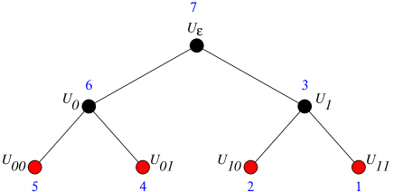
Fig. 3: This figure summarizes in which order we recover each codeword of a $\left(U\mid U+V\right)$ code of depth $2$. Nodes in red represent codes that are decoded with a soft information decoder, nodes in black correspond to codes that are not decoded directly and whose decoding is accomplished by first recovering the two descendants of the node and then combining them to recover the codeword we are looking for at this node.

When the constituent codes of this recursive $\left(U\mid U+V\right)$ construction are just codes of length $1$, it is readily seen that this decoding simply amounts to the successive cancellation decoder of Arıkan. We will be interested in the case where these constituent codes are longer than this. In such a case, we have to use as constituent codes, codes for which we have an efficient but possibly suboptimal decoder which can make use of soft information. Reed-Solomon codes or algebraic geometry codes with the Koetter Vardy decoder are precisely codes with this kind of property.

Polarization. The probability computations made during the $\left(U\mid U+V\right)$ decoding (1) and (2) correspond in a natural way to changing the channel model for the $U$ code and for the $V$ code. These two channels really correspond to the two channel combining models considered for polar codes. More precisely, if we consider a memoryless channel of input alphabet $\mathbb{F}_{q}$ and output alphabet $\mathcal{Y}$ defined by a transition matrix $W=(W(y|u))_{\begin{subarray}{c}u\in\mathbb{F}_{q}\\ y\in\mathbb{F}_{q}\end{subarray}}$, then the channel viewed by the $U$ decoder, respectively the $V$ decoder is a memoryless channel with transition matrix $W^{0}$ and $W^{1}$ respectively, which are given by

$$W^{0}(y_{1},y_{2},u_{2}|u_{1}) \stackrel{{\scriptstyle\text{def}}}{{=}} \frac{1}{q}W(y_{1}|u_{1})W(y_{2}|u_{1}\oplus u_{2})$$

$$W^{1}(y_{1},y_{2}|u_{2}) \stackrel{{\scriptstyle\text{def}}}{{=}} \frac{1}{q}\sum_{u_{1}\in\mathbb{F}_{q}}W(y_{1}|u_{1})W(y_{2}|u_{1}\oplus u_{2})$$

Here the $y^{\prime}_{i}$’s belong to $\mathcal{Y}$ and the $u_{i}$’s belong to $\mathbb{F}_{q}$. If we define the channel $W^{x}$ for $x=(x_{1}\dots x_{n})\in\{0,1\}^{n}$ recursively by

$$W^{x_{1}\dots x_{n-1}x_{n}}=\left(W^{x_{1}\dots x_{n-1}}\right)^{x_{n}}$$

then the channel viewed by the decoder for one of the constituent codes $U_{x_{1}\dots x_{n}}$ of an iterated $\left(U\mid U+V\right)$ code of depth $n$ (with the notation of Definition 2) is nothing but the channel $W^{x_{1}\dots x_{n}}$.

The key result used for showing that polar codes attain the capacity is that these channels polarize in the following sense

Theorem 1 ([ŞTA09, Theorem 1] and [Şaş11, Theorem 4.10]).

Let $q$ be an arbitrary prime. Then for a discrete $q$-ary input channel $W$ of symmetric capacity $C$ we have for all $0<\beta<\frac{1}{2}$

$$\lim_{\ell\rightarrow\infty}\frac{1}{n}\left|i\in\{0,1\}^{\ell}:{\mathcal{Z}\left(W^{i}\right)}\leq 2^{-n^{\beta}}\right|=C,$$

where $n\stackrel{{\scriptstyle\text{def}}}{{=}}2^{\ell}$.

Here ${\mathcal{Z}\left(W\right)}$ denotes the Bhattacharyya parameter of $W$ which is assumed to be a memoryless channel with $q$-ary inputs and outputs in an alphabet $\mathcal{Y}$. It is given by

$${\mathcal{Z}\left(W\right)}\stackrel{{\scriptstyle\text{def}}}{{=}}\frac{1}{q(q-1)}\sum_{x,x^{\prime}\in\mathbb{F}_{q},x^{\prime}\neq x}\sum_{y\in\mathcal{Y}}\sqrt{W(y|x)W(y|x^{\prime})}$$ (3)

Recall that this Bhattacharrya parameter quantifies the amount of noise in the channel. It is close to $0$ for channels with very low noise (i.e. channels of capacity close to $1$) whereas it is close to $1$ for very noisy channels (i.e. channels of capacity close to $0$).

3 Soft decoding of Reed-Solomon codes with the Koetter-Vardy decoding algorithm

It has been a long standing open problem to obtain an efficient soft-decision decoding algorithm for Reed-Solomon codes until Koetter and Vardy showed in [KV03a] how to modify appropriately the Guruswami-Sudan decoding algorithm in order to achieve this purpose. The complexity of this algorithm is polynomial and we will show here that the probability of error decreases exponentially in the codelength when the noise level is below a certain threshold. Let us first review a few basic facts about this decoding algorithm.

The reliability matrix.

The Koetter-Vardy decoder [KV03a] is based on a reliability matrix $\boldsymbol{\Pi}_{\mathbf{y}}$ of the codeword symbols $x(1),\dots,x(n)$ computed from the knowledge of the received word $\mathbf{y}$ and which is defined by

$$\boldsymbol{\Pi}_{\mathbf{y}}=\left(\textsf{prob}(x(j)=\alpha|y(j))\right)_{\begin{subarray}{c}\alpha\in\mathbb{F}_{q}\\ 1\leq j\leq n\end{subarray}}$$

Recall that the $j$-th column of this matrix $\boldsymbol{\Pi}_{\mathbf{y}}$ is denoted by $\boldsymbol{\Pi}_{\mathbf{y}}^{j}$. It gives the a posteriori probabilities (APP) that the $j$-th codeword symbol is equal to $\alpha$ where $\alpha$ ranges over $\mathbb{F}_{q}$.

We will be particularly interested in the $q$-ary symmetric channel model. The $q$-ary symmetric channel with error probability $p$, denoted by $q\hbox{-SC}_{p}$, takes a $q$-ary symbol at its input and outputs either the unchanged symbol, with probability $1-p$, or any of the other $q-1$ symbols, with probability $\tfrac{p}{q-1}$. Therefore, if the channel input symbols are uniformly distributed, the reliability matrix $\boldsymbol{\Pi}_{\mathbf{y}}$ for ${q\text{-SC}_{p}}$ is given by

$$\boldsymbol{\Pi}_{\mathbf{y}}^{j}(\alpha)=\textsf{prob}\left(x(j)=\alpha\mid y(j)\right)=\left\{\begin{array}[]{ll}1-p&\hbox{ if }\alpha=y(j)\\ \frac{p}{q-1}&\hbox{ if }\alpha\neq y(j)\end{array}\right.$$

Thus, all columns of $\boldsymbol{\Pi}_{\mathbf{y}}$ are identical up to permutation:

$$\boldsymbol{\Pi}_{\mathbf{y}}^{i}=\left(\begin{array}[]{c}1-p\\ \frac{p}{q-1}\\ \vdots\\ \frac{p}{q-1}\end{array}\right)\hbox{ (up to permutation)}$$

with $i=1,\ldots,n$.

This matrix is used by the Koetter-Vardy decoder to compute a multiplicity matrix that serves as the input to its soft interpolation step. When used in a $\left(U\mid U+V\right)$ construction and decoded as mentioned before, we will need to understand how the reliability matrix behaves through the $\left(U\mid U+V\right)$ decoding process. This is what we will do now.

Reliability matrix for the $V$-decoder.

We denote the reliability matrix of the $V$ decoder by $(\boldsymbol{\Pi}\oplus\boldsymbol{\Pi})_{\mathbf{y}}$ when $\boldsymbol{\Pi}_{\mathbf{y}_{1}}$ and $\boldsymbol{\Pi}_{\mathbf{y}_{2}}$ are the initial reliability matrices corresponding to the two halves of the received word $\mathbf{y}=(\mathbf{y}_{1},\mathbf{y}_{2})$. From the definition of the reliability matrix and (1) we readily obtain that

$$(\boldsymbol{\Pi}\oplus\boldsymbol{\Pi})_{\mathbf{y}}^{i}(\alpha)\stackrel{{\scriptstyle\text{def}}}{{=}}\sum_{\beta\in\mathbb{F}_{q}}\boldsymbol{\Pi}_{\mathbf{y}_{1}}^{i}(\beta)\cdot\boldsymbol{\Pi}_{\mathbf{y}_{2}}^{i}(\alpha-\beta).$$ (4)

Reliability matrix for the $U$-decoder

Similarly, by using (2) we see that the reliability matrix of the $U$ decoder, that we denote by $\boldsymbol{\Pi}\times\boldsymbol{\Pi}_{\mathbf{y},\mathbf{v}}$ is given by

$$(\boldsymbol{\Pi}\times\boldsymbol{\Pi})_{\mathbf{y},\mathbf{v}}^{i}(\alpha)=\frac{\boldsymbol{\Pi}_{\mathbf{y}_{1}}^{i}(\alpha)\cdot\boldsymbol{\Pi}_{\mathbf{\mathbf{y}}_{2}}^{i}(\alpha+v(i))}{\sum_{\beta\in\mathbb{F}_{q}}\boldsymbol{\Pi}_{\mathbf{\mathbf{y}}_{1}}^{i}(\beta)\cdot\boldsymbol{\Pi}_{\mathbf{\mathbf{y}}_{2}}^{i}(\beta+v(i))}.$$ (5)

To simplify notation we will generally avoid the dependency on $\mathbf{y}$ and $\mathbf{v}$ and simply write $\boldsymbol{\Pi}\oplus\boldsymbol{\Pi}$ and $\boldsymbol{\Pi}\times\boldsymbol{\Pi}$.

When does the Koetter-Vardy decoding algorithm succeed ?

Let us recall how the Koetter-Vardy soft decoder [KV03a] can be analyzed. By [KV03a, Theorem 12] their decoding algorithm outputs a list that contains the codeword $\mathbf{c}\in C$ if

$$\frac{\left\langle\boldsymbol{\Pi},\lfloor\mathbf{c}\rfloor\right\rangle}{\sqrt{\left\langle\boldsymbol{\Pi},\boldsymbol{\Pi}\right\rangle}}\geq\sqrt{k-1}+o(1)$$ (6)

as the codelength $n$ tends to infinity, where $\lfloor\mathbf{c}\rfloor$ represents a $q\times n$ matrix with entries $c_{i,\alpha}=1$ if $c_{i}=\alpha$, and $0$ otherwise; and $\left\langle\boldsymbol{A},\boldsymbol{B}\right\rangle$ denotes the inner product of the two $q\times n$ matrices $A$ and $B$, i.e.

$$\left\langle\boldsymbol{A},\boldsymbol{B}\right\rangle\stackrel{{\scriptstyle\text{def}}}{{=}}\sum_{i=1}^{q}\sum_{j=1}^{n}a_{i,j}b_{i,j}.$$

The algorithm uses a parameter $s$ (the total number of interpolation points counted with multiplicity). The little-O $o(1)$ depends on the choice of this parameter and the parameters $n$ and $q$.

We need a more precise formulation of the little-O of (6) to understand that we can get arbitrarily close to the lower bound $\sqrt{k-1}$ with polynomial complexity. In order to do so, let us provide more details about the Koetter Vardy decoding algorithm. Basically this algorithm starts by computing with Algorithm A of [KV03a, p.2814] from the knowledge of the reliability matrix $\boldsymbol{\Pi}$ and for the aforementioned integer parameter $s$ a $q\times n$ nonnegative integer matrix $\boldsymbol{M}(s)$ whose entries sum up to $s$. When $s$ goes to infinity $\boldsymbol{M}(s)$ becomes proportional to $\boldsymbol{\Pi}$. The cost of this matrix (we will drop the dependency in $s$) $C(\boldsymbol{M})$ is defined as

$$C(\boldsymbol{M})\stackrel{{\scriptstyle\text{def}}}{{=}}\frac{1}{2}\sum_{i=1}^{q}\sum_{j=1}^{n}m_{ij}(m_{ij}+1)=\frac{1}{2}\left(\left\langle\boldsymbol{M},\boldsymbol{M}\right\rangle+\left\langle\boldsymbol{M},\boldsymbol{1}\right\rangle\right)$$ (7)

where $m_{ij}$ denotes the entry of $\boldsymbol{M}$ at row $i$ and column $j$ and $\boldsymbol{1}$ is the all-one matrix. The complexity of the Koetter-Vardy decoding algorithm is dominated by solving a system of $C(\boldsymbol{M})$ linear equations. Then, the number of codewords on the list produced by the Koetter-Vardy decoder for a given multiplicity matrix $\boldsymbol{M}$ does not exceed

$$\mathcal{L}(\boldsymbol{M})\stackrel{{\scriptstyle\text{def}}}{{=}}\sqrt{\frac{2C(\boldsymbol{M})}{k-1}}.$$

It is straightforward to obtain from these considerations a soft-decision list decoder with a list which does not exceed some prescribed quantity $L$. Indeed it suffices to increase the value of $s$ in [KV03a, Algorithm A] until getting a matrix $\boldsymbol{M}$ which is such that

$$L\leq\mathcal{L}(\boldsymbol{M})<L+1$$

and to use this multiplicity matrix $\boldsymbol{M}$ in the Koetter-Vardy decoding algorithm. By following the terminology of [KV03a] we refer to this decoding procedure as algebraic soft-decoding with list size limited to $L$. [KV03a, Theorem 17] explains that convergence to the $\sqrt{k-1}$ lower-bound is at least as fast as $\mathcal{O}\left(1/L\right)$

Theorem 2 (Theorem 17, [KV03a]).

Algebraic soft-decoding with list size limited to $L$ produces a codeword $\mathbf{c}$ if

$$\frac{\left\langle\boldsymbol{\Pi},\lfloor\mathbf{c}\rfloor\right\rangle}{\sqrt{\left\langle\boldsymbol{\Pi},\boldsymbol{\Pi}\right\rangle}}\geq\frac{\sqrt{k-1}}{1-\frac{1}{L}\left(\frac{1}{R^{*}}+\frac{\sqrt{q}}{2\sqrt{R^{*}}}\right)}=\sqrt{k-1}\left(1+\mathcal{O}\left(\tfrac{1}{L}\right)\right)$$ (8)

where $R^{*}\stackrel{{\scriptstyle\text{def}}}{{=}}\frac{k-1}{n}$ and the constant in $\mathcal{O}\left(\cdot\right)$ depends only on $R^{*}$ and $q$.

Remark 2.

1. This theorem shows that the size of the list required to approach the asymptotic performance does not depend (directly) on the length of the code, it may depend on the rate of the code and the cardinality of the alphabet though.

2. As observed in [KV03a], this theorem is a very loose bound. The actual performance of algebraic soft-decoding with list size limited to $L$ is usually orders of magnitude better than that predicted by (8). A somewhat better bound is given by [KV03a, (44) p. 2819] where the condition for successful decoding $\mathbf{c}$ is

   $$\frac{\left\langle\boldsymbol{\Pi},\lfloor\mathbf{c}\rfloor\right\rangle}{\sqrt{\left\langle\boldsymbol{\Pi},\boldsymbol{\Pi}\right\rangle}} \geq \frac{\sqrt{k-1}}{1-\frac{1}{L}\left(\frac{1}{R^{*}}+\frac{\sqrt{n}}{2\sqrt{R^{*}\left\langle\boldsymbol{\Pi},\boldsymbol{\Pi}\right\rangle}}\right)}$$ (9)

   $$\approx \frac{\sqrt{k-1}}{1-\frac{1}{L}\left(\frac{1}{R^{*}}+\frac{1}{2\sqrt{R^{*}}}\right)}.$$

   where the approximation assumes that $\left\langle\boldsymbol{\Pi},\boldsymbol{\Pi}\right\rangle\approx n$ which holds for noise levels of practical interest. Note that this strengthens a little bit the constant in $\mathcal{O}\left(\cdot\right)$ that appears in Theorem 2, since it would not depend on $q$ anymore.

Decoding capability of the Koetter-Vardy decoder when the channel is symmetric.

The previous formula does not explain directly under which condition on the rate of the Reed-Solomon code decoding typically succeeds (in some sense this would be a “capacity” result for the Koetter-Vardy decoder). We will derive now such a result that appears to be new (but see the discussion at the end of this section). It will be convenient to restrict a little bit the class of memoryless channels we will consider- this will simplify formulas a great deal. The idea underlying this restriction is to make the behavior of the quantity $\left\langle\boldsymbol{\Pi},\lfloor\mathbf{c}\rfloor\right\rangle$ which appears in the condition of successful decoding (6) independent of the codeword $\mathbf{c}$ which is sent. This is readily obtained by restricting the channel to be weakly symmetric.

Definition 3 (weakly symmetric channel).

A discrete memoryless $W$ with input alphabet $\mathcal{X}$ and output alphabet $\mathcal{Y}$ is said to be weakly symmetric if and only if there is a partition of the output alphabet $\mathcal{Y}=Y_{1}\cup\dots\cup Y_{n}$ such that all the submatrices $W_{i}\stackrel{{\scriptstyle\text{def}}}{{=}}({W(y|x)})_{\begin{subarray}{c}x\in\mathcal{X}\\ y\in Y_{i}\end{subarray}}$ are symmetric. A matrix is said to be symmetric if all if its rows are permutations of each other, and all its columns are permutations of each other.

Remarks.

• Such a channel is called symmetric in [Gal68, p.94]. We avoid using the same terminology as Gallager since “symmetric channel” is generally used now to denote a channel for which any row is a permutation of each other row and the same property also holds for the columns.

• This notion is a generalization (when the output alphabet is discrete) of what is called a binary input symmetric channel in [RU08]. It also generalizes the notion of a cyclic symmetric channel in [BB06].

• It is shown that for such channels [Gal68, Th. 4.5.2] a uniform distribution on the inputs maximizes the mutual information between the output and the input of the channel and gives therefore its capacity. In such a case, linear codes attain the capacity of such a channel.

• This notion captures the notion of symmetry of a channel in a very broad sense. In particular the erasure channel is weakly symmetric (for many definitions of “symmetric channels” an erasure channel is not symmetric).

Notation 3.

We denote for such a channel and for a given output $y$ by $\pi_{y}=(\pi(\alpha))_{\alpha\in\mathbb{F}_{q}}$ the associated APP vector, that is $\pi(\alpha)=\textsf{prob}(x=\alpha|y)$ where we denote by $x$ the input symbol to the channel.

To compute this APP vector we will make throughout the paper the following assumption

Assumption 4.

The input of the communication channel is assumed to be uniformly distributed over $\mathbb{F}_{q}$.

We give now the asymptotic behavior of the Koetter-Vardy decoder for a weakly symmetric channel, but before doing this we will need a few lemmas.

Lemma 5.

Assume that $x$ is the input symbol that was sent and that the communication is weakly symmetric, then by viewing $\pi$ as a function of the random variable $y$ we have for any $x\in\mathbb{F}_{q}$:

$${\mathbb{E}}_{y}(\pi(x))={\mathbb{E}}_{y}\left(\left|\!\left|\pi\right|\!\right|^{2}\right),\leavevmode\nobreak\ \leavevmode\nobreak\ \leavevmode\nobreak\ \leavevmode\nobreak\ \hbox{ with }\left|\!\left|\pi\right|\!\right|^{2}\stackrel{{\scriptstyle\text{def}}}{{=}}\sum_{\alpha\in\mathbb{F}_{q}}\pi(\alpha)^{2}.$$

Proof.

To prove this result, let us introduce some notation. Let us denote by

• $\mathcal{Y}$ the output alphabet and $Y_{1}\cup\dots\cup Y_{n}=\mathcal{Y}$ is a partition of $\mathcal{Y}$ such that all the submatrices $W_{i}\stackrel{{\scriptstyle\text{def}}}{{=}}({W(y|x)})_{\begin{subarray}{c}x\in\mathcal{X}\\ y\in Y_{i}\end{subarray}}$ are symmetric for $i=1,\ldots,n$.

• $C_{i}\stackrel{{\scriptstyle\text{def}}}{{=}}\sum_{x\in\mathbb{F}_{q}}{W(y|x)}$ and $C_{i}^{(2)}\stackrel{{\scriptstyle\text{def}}}{{=}}\sum_{x\in\mathbb{F}_{q}}{W(y|x)}^{2}$ where $y$ is arbitrary in $Y_{i}$ (these quantities do not depend on the element $y$ chosen in $Y_{i}$);

• $R_{i}\stackrel{{\scriptstyle\text{def}}}{{=}}\sum_{y\in Y_{i}}{W(y|x)}$ and $R_{i}^{(2)}\stackrel{{\scriptstyle\text{def}}}{{=}}\sum_{y\in Y_{i}}{W(y|x)}^{2}$ where $x$ is arbitrary in $\mathbb{F}_{q}$.

We observe now that from the assumption that $x$ was uniformly distributed

$$\pi_{y}(\alpha)=\frac{\frac{1}{q}{W(y|\alpha)}}{\textsf{prob}(\text{receiving y})}=\frac{\frac{1}{q}{W(y|\alpha)}}{\frac{1}{q}\sum_{\beta\in\mathbb{F}_{q}}{W(y|\beta)}}=\frac{{W(y|\alpha)}}{\sum_{\beta\in\mathbb{F}_{q}}{W(y|\beta)}}.$$ (10)

We observe now that

$${\mathbb{E}}_{y}(\pi(x))=\sum_{y\in\mathcal{Y}}\pi_{y}(x){W(y|x)}=\sum_{y\in\mathcal{Y}}\frac{{W(y|x)}}{\sum_{\beta\in\mathbb{F}_{q}}{W(y|\beta)}}{W(y|x)}=\sum_{i=1}^{n}\sum_{y\in Y_{i}}\frac{{W(y|x)}^{2}}{\sum_{\beta\in\mathbb{F}_{q}}{W(y|\beta)}}=\sum_{i=1}^{n}\frac{R_{i}^{(2)}}{C_{i}}.$$

where the second equality is due to (10).

On the other hand

$${\mathbb{E}}_{y}\left(\left|\!\left|\pi\right|\!\right|^{2}\right) = \sum_{y\in\mathcal{Y}}\sum_{\alpha\in\mathbb{F}_{q}}\pi_{y}(\alpha)^{2}{W(y|x)}=\sum_{y\in\mathcal{Y}}\sum_{\alpha\in\mathbb{F}_{q}}\frac{{W(y|\alpha)}^{2}}{\left(\sum_{\beta\in\mathbb{F}_{q}}{W(y|\beta)}\right)^{2}}{W(y|x)}$$ (11)

$$= \sum_{i=1}^{n}\sum_{y\in Y_{i}}\sum_{\alpha\in\mathbb{F}_{q}}\frac{{W(y|\alpha)}^{2}}{\left(\sum_{\beta\in\mathbb{F}_{q}}{W(y|\beta)}\right)^{2}}{W(y|x)}=\sum_{i=1}^{n}\sum_{y\in Y_{i}}\sum_{\alpha\in\mathbb{F}_{q}}\frac{{W(y|\alpha)}^{2}}{(C_{i})^{2}}{W(y|x)}$$

$$= \sum_{i=1}^{n}\sum_{y\in Y_{i}}\frac{C_{i}^{(2)}}{(C_{i})^{2}}{W(y|x)}=\sum_{i=1}^{n}\frac{R_{i}C_{i}^{(2)}}{(C_{i})^{2}}$$

where the second equality is due to (10).

By summing all the elements (or the square of the elements) of the symmetric matrix $W_{i}$ either by columns or by rows and since all these row sums or all these column sums are equal, we obtain that

$$\sum_{\alpha\in\mathbb{F}_{q},y\in Y_{i}}{W(y|\alpha)}=|Y_{i}|C_{i}=qR_{i}$$

and

$$\sum_{\alpha\in\mathbb{F}_{q},y\in Y_{i}}{W(y|\alpha)}^{2}=|Y_{i}|C_{i}^{(2)}=qR^{(2)}_{i}$$

By using these two equalities in (11) we obtain

$${\mathbb{E}}_{y}\left(\left|\!\left|\pi\right|\!\right|^{2}\right)=\sum_{i=1}^{n}\frac{\frac{C_{i}|Y_{i}|}{q}\frac{R_{i}^{(2)}q}{|Y_{i}|}}{(C_{i})^{2}}=\sum_{i=1}^{n}\frac{R_{i}^{(2)}}{C_{i}}$$

This yields the same expression as the one for ${\mathbb{E}}_{y}(\pi(x))$ given in (3). ∎

As we will now show, this quantity ${\mathbb{E}}\left(\left|\!\left|\pi\right|\!\right|^{2}\right)$ turns out to be the limit of the rate for which the Koetter-Vardy decoder succeeds in decoding when the alphabet gets large. For this reason, we will denote this quantity by the Koetter-Vardy capacity of the channel.

Definition 4 (Koetter-Vardy capacity).

Consider a weakly symmetric channel and denote by $\pi$ the associated probability vector. The Koetter-Vardy capacity of this channel, which we denote by $C_{\text{KV}}$, is defined by

$$C_{\text{KV}}\stackrel{{\scriptstyle\text{def}}}{{=}}{\mathbb{E}}(\left|\!\left|\pi\right|\!\right|^{2}).$$

To prove that this quantity captures the rate at which the Koetter-Vardy is successful (at least for large lengths and therefore large field size) let us first prove concentration results around the expectation for the numerator and denominator appearing in the left-hand term of (6).

Lemma 6.

Let $\epsilon>0$ and $\mu\stackrel{{\scriptstyle\text{def}}}{{=}}{\mathbb{E}}(\left|\!\left|\pi\right|\!\right|^{2})$. We have

$$\textsf{prob}\left(\left\langle\boldsymbol{\Pi},\lfloor\mathbf{0}\rfloor\right\rangle\leq(1-\epsilon)\mu n\right) \leq e^{-2n\mu^{2}\epsilon^{2}}$$ (12)

$$\textsf{prob}\left(\left\langle\boldsymbol{\Pi},\boldsymbol{\Pi}\right\rangle\geq(1+\epsilon)n\mu\right) \leq e^{-2n\mu^{2}\epsilon^{2}}$$ (13)

Proof.

Let us first prove (13). We can write the left-hand term as a sum of $n$ i.i.d. random variables

$$\left\langle\boldsymbol{\Pi},\boldsymbol{\Pi}\right\rangle=\sum_{j=1}^{n}X_{j},$$

where $X_{j}\stackrel{{\scriptstyle\text{def}}}{{=}}\left|\!\left|\boldsymbol{\Pi}(j)\right|\!\right|^{2}$. Note that (i) ${\mathbb{E}}\left(X_{j}\right)={\mathbb{E}}(\left|\!\left|\pi\right|\!\right|^{2})$, (ii) $0\leq X_{j}\leq 1$. By using Hoeffding’s inequality we obtain that for any $\epsilon>0$ we have

$$\textsf{prob}\left(\sum_{j=1}^{n}X_{j}\geq n\mu(1+\epsilon)\right)\leq e^{-2n\mu^{2}\epsilon^{2}}.$$ (14)

Now (12) can be dealt with in a similar way by writing

$$\left\langle\boldsymbol{\Pi},\lfloor\boldsymbol{0}\rfloor\right\rangle=\sum_{j=1}^{n}Y_{j}$$

where $Y_{j}\stackrel{{\scriptstyle\text{def}}}{{=}}\Pi^{j}(0)$. The channel is assumed to be symmetric and we can therefore use Lemma 5 from which we deduce that ${\mathbb{E}}(Y_{j})={\mathbb{E}}(\left|\!\left|\pi\right|\!\right|^{2})=\mu$. We also have $0\leq Y_{j}\leq 1$ and by applying Hoeffding’s inequality we obtain that for any $\epsilon>0$ we have

$$\textsf{prob}\left(\sum_{j=1}^{n}Y_{j}\leq n\mu(1-\epsilon)\right)\leq e^{-2n\mu^{2}\epsilon^{2}}.$$ (15)

∎

This result can be used to derive a rather tight upper-bound on the probability of error of the Koetter-Vardy decoder.

Theorem 7.

Consider a weakly symmetric $q$-ary input channel of Koetter-Vardy capacity $C_{\text{KV}}$. Consider a Reed-Solomon code over $\mathbb{F}_{q}$ of length $n$, dimension $k$ such that its rate $R=\frac{k}{n}$ satisfies $R<C_{\text{KV}}$. Let

$$\delta \stackrel{{\scriptstyle\text{def}}}{{=}} \frac{C_{\text{KV}}-R}{R}$$

$$R^{*} \stackrel{{\scriptstyle\text{def}}}{{=}} \frac{k-1}{n}$$

$$L \stackrel{{\scriptstyle\text{def}}}{{=}} \left\lceil\frac{3\left(\frac{1}{R^{*}}+\frac{\sqrt{q}}{2\sqrt{R^{*}}}\right)(1+\tfrac{\delta}{3})}{\delta}\right\rceil$$

The probability that the Koetter-Vardy decoder with list size bounded by $L$ does not output in its list the right codeword is upper-bounded by $\mathcal{O}\left(e^{-K\delta^{2}n}\right)$ for some constant $K$.

Proof.

Without loss of generality we can assume that the all-zero codeword $\boldsymbol{0}$ was sent. From Theorem 2, we know that the Koetter-Vardy decoder succeeds if and only if the following condition is met

$$\frac{\left\langle\boldsymbol{\Pi},\lfloor\mathbf{0}\rfloor\right\rangle}{\sqrt{\left\langle\boldsymbol{\Pi},\boldsymbol{\Pi}\right\rangle}}\geq\frac{\sqrt{k-1}}{1-\frac{1}{L}\left(\frac{1}{R^{*}}+\frac{\sqrt{q}}{2\sqrt{R^{*}}}\right)}.$$

Notice that the right-hand side satisfies

$$\frac{\sqrt{k-1}}{1-\frac{1}{L}\left(\frac{1}{R^{*}}+\frac{\sqrt{q}}{2\sqrt{R^{*}}}\right)}\leq\frac{\sqrt{k-1}}{1-\frac{\delta\left(\frac{1}{R^{*}}+\frac{\sqrt{q}}{2\sqrt{R^{*}}}\right)}{3\left(\frac{1}{R^{*}}+\frac{\sqrt{q}}{2\sqrt{R^{*}}}\right)\left(1+\tfrac{\delta}{3}\right)}}=\frac{\sqrt{k-1}}{1-\frac{\delta}{3+\delta}}=\sqrt{k-1}\left(1+\tfrac{\delta}{3}\right)$$ (16)

Let $\epsilon$ be a positive constant that we are going to choose afterward. Define the events $\mathcal{E}_{1}$ and $\mathcal{E}_{2}$ by

$$\mathcal{E}_{1} \stackrel{{\scriptstyle\text{def}}}{{=}} \{\boldsymbol{\Pi}:\left\langle\boldsymbol{\Pi},\boldsymbol{\Pi}\right\rangle\leq nC_{\text{KV}}(1+\epsilon)\}$$

$$\mathcal{E}_{2} \stackrel{{\scriptstyle\text{def}}}{{=}} \{\boldsymbol{\Pi}:\left\langle\boldsymbol{\Pi},\lfloor\boldsymbol{0}\rfloor\right\rangle\geq nC_{\text{KV}}(1-\epsilon)\}.$$

Note that by Lemma 6 the events $\mathcal{E}_{1}$ and $\mathcal{E}_{2}$ have both probability $\geq 1-\epsilon^{\prime}$ where $\epsilon^{\prime}\stackrel{{\scriptstyle\text{def}}}{{=}}e^{-2nC_{\text{KV}}^{2}\epsilon^{2}}$.

Thus, the probability that event $\mathcal{E}_{1}$ and event $\mathcal{E}_{2}$ both occur is

$$\textsf{prob}(\mathcal{E}_{1}\cap\mathcal{E}_{2})=\textsf{prob}(\mathcal{E}_{1})+\textsf{prob}(\mathcal{E}_{2})-\textsf{prob}(\mathcal{E}_{1}\cup\mathcal{E}_{2})\geq 1-\epsilon^{\prime}+1-\epsilon^{\prime}-1=1-2\epsilon^{\prime}.$$

In the case $\mathcal{E}_{1}$ and $\mathcal{E}_{2}$ both hold, we have

$$\frac{\left\langle\boldsymbol{\Pi},\lfloor\mathbf{0}\rfloor\right\rangle}{\sqrt{\left\langle\boldsymbol{\Pi},\boldsymbol{\Pi}\right\rangle}}\geq\frac{1-\epsilon}{\sqrt{1+\epsilon}}\sqrt{C_{\text{KV}}n}$$ (17)

A straightforward computation shows that for any $x>0$ we have

$$\frac{1-x}{\sqrt{1+x}}\geq 1-\frac{3}{2}x.$$

Therefore for $\epsilon>0$ we have in the aforementioned case

$$\frac{\left\langle\boldsymbol{\Pi},\lfloor\mathbf{0}\rfloor\right\rangle}{\sqrt{\left\langle\boldsymbol{\Pi},\boldsymbol{\Pi}\right\rangle}}\geq\left(1-\tfrac{3}{2}\epsilon\right)\sqrt{C_{\text{KV}}n}=\left(1-\tfrac{3}{2}\epsilon\right)\sqrt{(1+\delta)Rn}=\left(1-\tfrac{3}{2}\epsilon\right)\sqrt{k(1+\delta)}$$

Let us choose now $\epsilon$ such that

$$\left(1-\tfrac{3}{2}\epsilon\right)\sqrt{1+\delta}=1+\tfrac{\delta}{3}.$$ (18)

Note that $\epsilon=\Theta(\delta)$. This choice implies that

$$\frac{\left\langle\boldsymbol{\Pi},\lfloor\mathbf{0}\rfloor\right\rangle}{\sqrt{\left\langle\boldsymbol{\Pi},\boldsymbol{\Pi}\right\rangle}}\geq\sqrt{k}\left(1+\tfrac{\delta}{3}\right)\geq\sqrt{k-1}\left(1+\tfrac{\delta}{3}\right)\geq\frac{\sqrt{k-1}}{1-\frac{1}{L}\left(\frac{1}{R^{*}}+\frac{\sqrt{q}}{2\sqrt{R^{*}}}\right)}$$

where we used in the last inequality the bound given in (16).

In other words, the Koetter Vardy decoder outputs the codeword $\boldsymbol{0}$ in its list. The probability that this does not happen is at most $2e^{-2nC_{\text{KV}}^{2}\epsilon^{2}}=e^{-n\Theta(\delta^{2})}$. ∎

An immediate corollary of this theorem is the following result that gives a (tight) lower bound on the error-correction capacity of the Koetter-Vardy decoding algorithm over a discrete memoryless channel.

Corollary 8.

Let $(\mathscr{C}_{n})_{n\geq 1}$ be an infinite family of Reed-Solomon codes of rate $\leq R$. Denote by $q_{n}$ the alphabet size of $\mathscr{C}_{n}$ that is assumed to be a non decreasing sequence that goes to infinity with $n$. Consider an infinite family of $q_{n}$-ary weakly symmetric channels with associated probability error vectors $\pi_{n}$ such that ${\mathbb{E}}\left(\left|\!\left|\pi_{n}\right|\!\right|^{2}\right)$ has a limit as $n$ tends to infinity. Denote by $C_{\text{KV}}^{\infty}$ the asymptotic Koetter-Vardy capacity of these channels, i.e.

$$C_{\text{KV}}^{\infty}\stackrel{{\scriptstyle\text{def}}}{{=}}\lim_{n\rightarrow\infty}{\mathbb{E}}\left(\left|\!\left|\pi_{n}\right|\!\right|^{2}\right).$$

This infinite family of codes can be decoded correctly by the Koetter-Vardy decoding algorithm with probability $1-o(1)$ as $n$ tends to infinity as soon as there exists $\epsilon>0$ such that

$$R\leq C_{\text{KV}}^{\infty}-\epsilon.$$

Remark 3.

Let us observe that for the $q\hbox{-SC}_{p}$ we have

$${\mathbb{E}}\left(\left|\!\left|\pi\right|\!\right|^{2}\right)=(1-p)^{2}+(q-1)\frac{p^{2}}{(q-1)^{2}}=(1-p)^{2}+\mathcal{O}\left(\frac{1}{q}\right).$$

By letting $q$ going to infinity, we recover in this way the performance of the Guruswami-Sudan algorithm which works as soon as $R<(1-p)^{2}$.

Link with the results presented in [KV03a] and [KV03b]. In [KV03a, Sec. V.B eq. (32)] an arbitrarily small upper bound on the error probability $P_{e}$ is given, it is namely explained that $P_{e}\leq\epsilon$ as soon as the rate $R$ and the length $n$ of the Reed-Solomon code satisfy $\sqrt{R}\leq{\mathbb{E}}(\mathcal{Z}^{*})-\frac{1}{\sqrt{\epsilon n}}$ (where the expectation is taken with respect to the a posteriori probability distribution of the codeword). Here $\mathcal{Z}^{*}$ is some function of the multiplicity matrix which itself depends on the received word. This is not a bound of the same form as the one given in Theorem 7 whose upper-bound on the error probability only depends on some well defined quantities which govern the complexity of the algorithm (such as the size $q$ of the field over which the Reed-Solomon code is defined and a bound on the list-size) and the Koetter-Vardy capacity of the channel.

However, many more details are given in the preprint version [KV03b] of [KV03a] in Section 9. There is for instance implicitly in the proof of Theorem 27 in [KV03b, Sec. 9] an upper-bound on the error probability of decoding a Reed-Solomon code with the Koetter-Vardy decoder which goes to zero polynomially fast in the length as long as the rate is less than $C\stackrel{{\scriptstyle\text{def}}}{{=}}\frac{\operatorname{trace}\left(W(\operatorname{diag}P_{Y})^{-1}W^{T}\right)}{q^{2}}$ where $W$ is the transition probability matrix of the channel and $\operatorname{diag}P_{Y}$ is the $|\mathcal{Y}|\times|\mathcal{Y}|$ matrix which is zero except on the diagonal where the diagonal elements give the probability distribution of the output of the channel when the input is uniformly distributed. It is readily verified that in the case of a weakly symmetric channel $C$ is nothing but the Koetter-Vardy capacity of the channel defined here. $C$ can be viewed as a more general definition of the “capacity” of a channel adapted to the Koetter-Vardy decoding algorithm. However it should be said that “error-probability” in [KV03a, KV03b] should be understood here as “average error probability of error” where the average is taken over the set of codewords of the code. It should be said that this average may vary wildly among the codewords in the case of a non-symmetric channel. In order to avoid this, we have chosen a different route here and have assumed some weak form of symmetry for the channel which ensures that the probability of error does not depend on the codeword which is sent. The authors of [KV03b] use a second moment method to bound the error probability, this can only give polynomial upper-bounds on the error probability. This is why we have also used a slightly different route in Theorem 7 to obtain stronger (i.e. exponentially small) upper-bounds on the error probability.

4 Algebraic-soft decision decoding of AG codes.

The problem with Reed-Solomon codes is that their length is limited by the alphabet size. To overcome this limitation it is possible to proceed as in [KV03b] and use instead Algebraic-Geometric codes (AG codes in short) which can also be decoded by an extension of the Koetter-Vardy algorithm and which have more or less a similar error correction capacity as Reed-Solomon codes under this decoding strategy. The extension of this decoding algorithm to AG codes is sketched in Section D. Let us first recall how these codes are defined.

An AG code is constructed from a triple $(\mathcal{X},\mathcal{P},mQ)$ where:

• $\mathcal{X}$ denotes an algebraic curve over a finite field $\mathbb{F}_{q}$ (we refer to [Sti93] for more information about algebraic geometry codes);

• $\mathcal{P}=\left\{P_{1},\ldots,P_{n}\right\}$ denotes a set of $n$ distinct points of $\mathcal{X}$ with coordinates in $\mathbb{F}_{q}$;

• $mQ$ is a divisor of the curve, here $Q$ denotes another point in $\mathcal{X}$ with coordinates in $\mathbb{F}_{q}$ which is not in $\mathcal{P}$ and $m$ is a nonnegative integer.

We define $\mathcal{L}(mQ)$ as the vector space of rational functions on $\mathcal{X}$ that may contain only a pole at $Q$ and the multiplicity of this pole is at most $m$. Then, the algebraic geometry code associated to the above triple denoted by $\mathcal{C}_{L}(\mathcal{X},\mathcal{P},{mQ})$ is the image of $\mathcal{L}(mQ)$ under the evaluation map $\begin{array}[]{cccc}\mathrm{ev}_{\mathcal{P}}:&\mathcal{L}(mQ)&\longrightarrow&\mathbb{F}_{q}^{n}\end{array}$ defined by $\mathrm{ev}_{\mathcal{P}}(f)=\left(f(P_{1}),\ldots,f(P_{n})\right)$, i.e.

$$\mathcal{C}_{L}(\mathcal{X},\mathcal{P},{mQ})\stackrel{{\scriptstyle\text{def}}}{{=}}\left\{\mathrm{ev}_{\mathcal{P}}(f)=\left(f(P_{1}),\ldots,f(P_{n})\right)\mid f\in\mathcal{L}(mQ)\right\}$$

Since the evaluation map is linear, the code $\mathcal{C}_{L}(\mathcal{X},\mathcal{P},{mQ})$ is a linear code of length $n$ over $\mathbb{F}_{q}$ and dimension $k=\dim(\mathcal{L}(mQ))$. This dimension can be lower bounded by $k\geq m-g+1$ where $g$ is the genus of the curve. Recall that this quantity is defined by

$$g\stackrel{{\scriptstyle\text{def}}}{{=}}\max_{m\geq 0}\{m-\dim\mathcal{L}(mQ)\}+1$$

Moreover the minimum distance $d$ of this code satisfies $d\geq n-m$.

Reed-Solomon codes are a particular case of the family of AG codes and correspond to the case where $\mathcal{X}$ is the affine line over $\mathbb{F}_{q}$, $\mathcal{P}$ are $n$ distinct elements of $\mathbb{F}_{q}$ and $\mathcal{L}$ is the vector space of polynomials of degree at most $k-1$ and with coefficients in $\mathbb{F}_{q}$.

Recall that it is possible to obtain for any designed rate $R=\tfrac{k}{n}$ and any square prime power $q$ an infinite family of AG codes over $\mathbb{F}_{q}$ of rate $\geq R$ of increasing length $n$ and minimum distance $d$ meeting “asymptotically” the MDS bound as $q$ goes to infinity

$$\frac{d}{n}\geq(1-R)-O\left(\frac{1}{\sqrt{q}}\right)$$

This follows directly from the two aforementioned lower bounds $k\geq m-g+1$ and $d\geq n-m$ and the well known result of Tsfasman, Vlăduts and Zink [TVZ82]

Theorem 9 ([TVZ82]).

For any number $R\in[0,1]$ and any square prime power $q$ there exists an infinite family of AG codes over $\mathbb{F}_{q}$ of rate $\geq R$ of increasing length $n$ such that the normalized genus $\gamma\stackrel{{\scriptstyle\text{def}}}{{=}}\frac{g}{n}$ of the underlying curve satisfies

$$\gamma\leq\frac{1}{\sqrt{q}-1}$$

We will call such codes Tsfasman-Vlăduts-Zink AG codes in what follows.

As is done in [KV03b], it will be helpful to assume that $2g-1\leq m<n$. This implies among other things that the dimension of the code is given my $k=m-g+1$. $k=m-g+1$ We will make this assumption from now on. As in [KV03a] it is possible to obtain a soft-decision list decoder with a list which does not exceed some prescribed quantity $L$. Similar to the Reed- Solomon case considered in [KV03a], it suffices to increase the value of $s$ in [KV03a][Algorithm A] until we get a matrix $\boldsymbol{M}$ such that $L<L_{m}(\boldsymbol{M})<L+1$, where $L(\boldsymbol{M})$ is a bound on the list of the codewords output by the algorithm which is given in Lemma 32, and then to use this matrix $\boldsymbol{M}$ in the Koetter Vardy decoding algorithm.

The following result is similar to [KV03a, Th. 17]

Theorem 10.

Algebraic soft-decoding for AG codes with list-size limited to $L$ produces a list that contains a codeword $\mathbf{c}\in\mathcal{C}_{L}(\mathcal{X},\mathcal{P},{mQ})$ if

$$\frac{\left\langle\boldsymbol{\Pi},\lfloor\mathbf{c}\rfloor\right\rangle}{\sqrt{\left\langle\boldsymbol{\Pi},\boldsymbol{\Pi}\right\rangle}}\geq\sqrt{m}\frac{1+\frac{\tilde{\gamma}+\sqrt{2\tilde{\gamma}}}{L\sqrt{1-\tfrac{2\tilde{\gamma}}{L}\left(1+\tfrac{2}{L}\right)}}}{1-\frac{1}{L\sqrt{1-\tfrac{2\tilde{\gamma}}{L}\left(1+\tfrac{2}{L}\right)}}\left(\frac{\sqrt{q}}{2\sqrt{\tilde{R}}}+\frac{1}{\tilde{R}}\right)}=\sqrt{m}\left(1+\mathcal{O}\left(\frac{1}{L}\right)\right)$$ (19)

where $\tilde{R}=\frac{m}{n}$, $\tilde{\gamma}=\frac{g}{m}$ and $\mathcal{O}(\cdot)$ depends only on $\tilde{R}$, $\tilde{g}$ and $q$.

The proof of this theorem can be found in Section D of the appendix. It heavily relies on results proved in the preprint version [KV03b] of [KV03a].

Theorem 11.

Consider a weakly symmetric $q$-ary input channel of Koetter-Vardy capacity $C_{\text{KV}}$ where $q$ is a square prime power. Consider a Tsfasman-Vlăduts-Zink AG code over $\mathbb{F}_{q}$ of length $n$, dimension $k$ such that its rate $R=\frac{k}{n}$ satisfies $R<C_{\text{KV}}-\gamma$ where $\gamma\stackrel{{\scriptstyle\text{def}}}{{=}}\frac{1}{\sqrt{q}-1}$. Let

$$\delta \stackrel{{\scriptstyle\text{def}}}{{=}} \frac{C_{\text{KV}}-R-\gamma}{R}$$

$$\tilde{R} \stackrel{{\scriptstyle\text{def}}}{{=}} \frac{m}{n}$$

$$\tilde{\gamma} \stackrel{{\scriptstyle\text{def}}}{{=}} \frac{g}{m}$$

$$f(\ell) \stackrel{{\scriptstyle\text{def}}}{{=}} \frac{1+\frac{\tilde{\gamma}+\sqrt{2\tilde{\gamma}}}{\ell\sqrt{1-\tfrac{2\tilde{\gamma}}{\ell}\left(1+\tfrac{2}{\ell}\right)}}}{1-\frac{1}{\ell\sqrt{1-\tfrac{2\tilde{\gamma}}{L}\left(1+\tfrac{2}{\ell}\right)}}\left(\frac{\sqrt{q}}{2\sqrt{\tilde{R}}}+\frac{1}{\tilde{R}}\right)}$$

$$L \stackrel{{\scriptstyle\text{def}}}{{=}} f^{-1}\left(1+\frac{\delta}{3}\right)$$

The probability that the Koetter-Vardy decoder with list size bounded by $L$ does not output in its list the right codeword is upper-bounded by

$$\mathcal{O}\left(e^{-K\delta^{2}n}\right)$$

for some constant $K$. Moreover $L=\Theta\left(1/\delta\right)$ as $\delta$ tends to zero.

Proof.

The proof follows word by word the proof of Theorem 7 with the only difference that $k-1$ is replaced by $m=k+g$. The only new ingredient is that we use Theorem 10 instead of (8) which explains the new form chosen for the list-size $L$. The last part, namely that $L=\Theta\left(1/\delta\right)$ is a simple consequence of the fact that $f(L)=1+\Theta\left(\frac{1}{L}\right)$ as $L$ tends to infinity. ∎

5 Correcting errors beyond the Guruswami-Sudan bound

The purpose of this section is to show that the $\left(U\mid U+V\right)$ construction improves significantly the noise level that the Koetter-Vardy decoder is able to correct. To be more specific, consider the $q$-ary symmetric channel. The asymptotic Koetter-Vardy capacity of a family of $q$-ary symmetric channels of crossover probability $p$ is equal to $(1-p)^{2}$. It turns out that this is also the maximum crossover probability that the Guruswami-Sudan decoder is able to sustain when the alphabet and the length go to infinity. We will prove here that the $\left(U\mid U+V\right)$ construction with Reed-Solomon components already performs a bit better than $(1-p)^{2}$ when the rate is small enough. By using iterated $\left(U\mid U+V\right)$ constructions we will be able to improve rather significantly the performances and this even for a moderate number of levels.

Our analysis of the Koetter-Vardy decoding is done for weakly symmetric channels. When we want to analyze a $\left(U\mid U+V\right)$ code based on Reed-Solomon codes used over a channel $W$ it will be helpful that the channels $W^{0}$ and $W^{1}$ viewed by the decoder of $U$ and $V$ respectively are also weakly symmetric. Simple examples show that this is not necessarily the case. However a slight restriction of the notion of weakly symmetric channel considered in [BB06] does the job. It consists in the notion of a cyclic-symmetric channel whose definition is given below.

Definition 5 (cyclic-symmetric channel).

We denote for a vector $\mathbf{y}=(y_{i})_{i\in\mathbb{F}_{q}}$ with coordinates indexed by a finite field $\mathbb{F}_{q}$ by $\mathbf{y}^{+g}$ the vector $\mathbf{y}^{+g}=(y_{i+g})_{i\in\mathbb{F}_{q}}$, by $n(\mathbf{y})$ the number of $g$’s in $\mathbb{F}_{q}$ such that $\mathbf{y}^{+g}=\mathbf{y}$ and by $\mathbf{y}^{*}$ the set $\{\mathbf{y}^{+g},g\in\mathbb{F}_{q}\}$. A $q$-ary input channel is cyclic-symmetric channel if and only there exists a probability function $Q$ defined over the sets of possible $\pi^{*}$ such that for any $i\in\mathbb{F}_{q}$ we have

$$\textsf{prob}(\pi=\mathbf{y}|x=i)=y_{i}n(\mathbf{y})Q(\mathbf{y}^{*}).$$

The point about this notion is that $W^{0}$ and $W^{1}$ stay cyclic-symmetric when $W$ is cyclic-symmetric and that a cyclic-symmetric channel is also weakly symmetric. This will allow to analyze the asymptotic error correction capacity of iterated $\left(U\mid U+V\right)$ constructions.

Proposition 12 ([BB06]).

Let $W$ be a cylic-symmetric channel. Then $W$ is weakly symmetric and $W^{0}$ and $W^{1}$ are also cyclic-symmetric.

5.1 The $\left(U\mid U+V\right)$-construction

We study here how a $\left(U\mid U+V\right)$ code performs when $U$ and $V$ are both Reed-Solomon codes decoded with the Koetter-Vardy decoding algorithm when the communication channel is a $q$-ary symmetric channel of error probability $p$.

Proposition 13.

For any real $p$ in $[0,1]$ and real $R$ such that

$$R<C^{\infty}_{\left(U\mid U+V\right)}(p)\stackrel{{\scriptstyle\text{def}}}{{=}}\frac{(p^{3}-4p^{2}+4p-4)(1-p)^{2}}{2(p-2)},$$

there exists an infinite family of $\left(U\mid U+V\right)$-codes of rate $\geq R$ based on Reed-Solomon codes whose alphabet size $q$ increases with the length and whose probability of error on the ${q\text{-SC}_{p}}$ when decoded by the iterated $\left(U\mid U+V\right)$-decoder based on the Koetter-Vardy decoding algorithm goes to $0$ with the alphabet size.

Proof.

The $(U_{0}|U_{0}+U_{1})$-construction can be decoded correctly by the Koetter-Vardy decoding algorithm if it decodes correctly $U_{0}$ and $U_{1}$. Let $\pi_{i}$ be the APP probability vector seen by the decoder for $U_{i}$ for $i\in\{0,1\}$. A ${q\text{-SC}_{p}}$ is clearly a cyclic-symmetric channel and therefore the channel viewed by the $U_{0}$ decoder and the $U_{1}$ decoder are also cyclic-symmetric by Proposition 12. A cyclic-symmetric channel is weakly symmetric and therefore by Corollary 8, decoding succeeds with probability $1-o(1)$ when we choose the rate $R_{i}$ of $U_{i}$ to be any positive number below $\lim_{q\rightarrow\infty}{\mathbb{E}}\left(\left|\!\left|\pi_{i}\right|\!\right|^{2}\right)$ for $i\in\{0,1\}$.

In Section A of the appendix it is proved in Lemmas 21 and 22 that

$${\mathbb{E}}\left(\left|\!\left|\pi_{0}\right|\!\right|^{2}\right) = \frac{(p+2)(p-1)^{2}}{2-p}+\mathcal{O}\left(\frac{1}{q}\right)$$

$${\mathbb{E}}\left(\left|\!\left|\pi_{1}\right|\!\right|^{2}\right) = (1-p)^{4}+\mathcal{O}\left(\frac{1}{q}\right)$$

Since the rate $R$ of the $\left(U\mid U+V\right)$ construction is equal to $\frac{R_{0}+R_{1}}{2}$ decoding succeeds with probabilty $1-o(1)$ if

$$R<\lim_{q\rightarrow\infty}\frac{{\mathbb{E}}\left(\left|\!\left|\pi_{0}\right|\!\right|^{2}\right)+{\mathbb{E}}\left(\left|\!\left|\pi_{1}\right|\!\right|^{2}\right)}{2}=\frac{(p^{3}-4p^{2}+4p-4)(1-p)^{2}}{2(p-2)}.$$

∎

From Figure 4 we deduce that the $\left(U\mid U+V\right)$ decoder outperforms the RS decoder with Guruswami-Sudan or Koetter-Vardy decoders as soon as $R<0.17$.

5.2 Iterated $\left(U\mid U+V\right)$-construction

Now we will study what happens over a $q$-ary symmetric channel with error probability $p$ if we apply the iterated $\left(U\mid U+V\right)$-construction with Reed-Solomon codes as constituent codes. In particular, the following result handles the cases of the iterated $\left(U\mid U+V\right)$-construction of depth $2$ and $3$.

Proposition 14.

For any real $p$ in $[0,1]$ we define

$$C^{\infty,(2)}_{\left(U\mid U+V\right)}(p)\stackrel{{\scriptstyle\text{def}}}{{=}}\frac{Q(p)(1-p)^{2}}{4(p^{2}-2p+2)(3p-4)(2-p)^{2}}$$ (20)

and

$$C^{\infty,(3)}_{\left(U\mid U+V\right)}(p)\stackrel{{\scriptstyle\text{def}}}{{=}}\frac{S(p)(1-p)^{2}}{T_{1}(p)T_{2}(p)T_{3}(p)\left(3p^{2}-6p+4\right)\left(p^{2}-2p+2\right)^{2}\left(7p-8\right)\left(3p-4\right)^{2}\left(2-p\right)^{4}}$$ (21)

Then, for any real $R$ such that $R<C^{\infty,(2)}_{\left(U\mid U+V\right)}(p)$ (resp. $R<C^{\infty,(3)}_{\left(U\mid U+V\right)}(p)$) there exists an infinite family of iterated $\left(U\mid U+V\right)$-codes of depth $2$ (resp. of depth $3$) and rate $\geq R$ based on Reed-Solomon codes whose alphabet size $q$ increases with the length and whose probability of error with the Koetter-Vardy decoding algorithm goes to $0$ with the alphabet size.

Where

$$Q(p) \stackrel{{\scriptstyle\text{def}}}{{=}} 3p^{11}-40p^{10}+243p^{9}-890p^{8}+2192p^{7}-3800p^{6}+4702p^{5}-4148p^{4}+2624p^{3}-1248p^{2}+480p-128,$$

$$T_{1}(p) \stackrel{{\scriptstyle\text{def}}}{{=}} p^{4}-4p^{3}+6p^{2}-4p+2,$$

$$T_{2}(p) \stackrel{{\scriptstyle\text{def}}}{{=}} 7p^{2}-18p+12,$$

$$T_{3}(p) \stackrel{{\scriptstyle\text{def}}}{{=}} 5p^{2}-12p+8\hbox{ and }$$

$$S(p) \stackrel{{\scriptstyle\text{def}}}{{=}} 6615p^{35}-269766p^{34}+5348715p^{33}-68697432p^{32}+642499307p^{31}-4663447618p^{30}+27338551153p^{29}$$

$$- 133009675740p^{28}+547673160274p^{27}-1936548054764p^{26}+5946432348816p^{25}-15994984917120p^{24}$$

$$+ 37947048851166p^{23}-79831430926900p^{22}+149553041935846p^{21}-250287141028584p^{20}+375085789739404p^{19}$$

$$- 504157479736392p^{18}+608316727420536p^{17}-659027903954592p^{16}+640716590979968p^{15}-558310438932224p^{14}$$

$$+ 435164216863552p^{13}-302519286136704p^{12}+186871196449024p^{11}-102093104278528p^{10}+49062052366336p^{9}$$

$$- 20617356455936p^{8}+7534906109952p^{7}-2386429566976p^{6}+655237726208p^{5}-156569829376p^{4}$$

$$+ 32471121920p^{3}-5628755968p^{2}+723517440p-50331648$$

Proof.

The proof is given in Appendix B and C for iterated $\left(U\mid U+V\right)$ construction of depth $2$ and $3$, respectively. ∎

Figure 4 summarizes the performances of these iterated $\left(U\mid U+V\right)$-constructions From this figure we see that if we apply the iterated $\left(U\mid U+V\right)$-construction of depth $2$ we get better performance than decoding a classical Reed-Solomon code with the Guruswami-Sudan decoder for low rate codes, specifically for $R<0.325$. Moreover, if we apply the iterated $\left(U\mid U+V\right)$-construction of depth $3$ we get even better results, we beat the Guruswami-Sudan for codes of rate $R<0.475$.

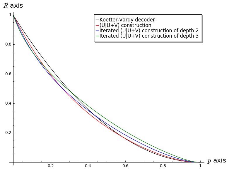
Fig. 4: Rate plotted against the crossover error probability $p$ for four code-constructions. The black line refers to standard Reed-Solomon codes decoded by the Guruswami-Sudan algorithm, the red line to the $\left(U\mid U+V\right)$-construction, the blue line to the iterated $\left(U\mid U+V\right)$-construction of depth $2$ and the green line to the iterated $\left(U\mid U+V\right)$-construction of depth $3$.

5.3 Finite length capacity

Even if for finite alphabet size $q$ the Koetter-Vardy capacity cannot be understood as a capacity in the usual sense: no family of codes is known which could be decoded with the Koetter-Vardy decoding algorithm and whose probability of error would go to zero as the codelength goes to infinity at any rate below the Koetter-Vardy capacity. Something like that is only true approximately for AG codes when the size of the alphabet is a square prime power and if we are willing to pay an additional term of $\frac{1}{\sqrt{q}-1}$ in the gap between the Koetter-Vardy capacity and the actual code rate. Actually, we can even be sure that for certain rates this result can not hold, since the Koetter-Vardy capacity can be above the Shannon capacity for very noisy channels. Consider for instance the “completely-noisy” $q$-ary symmetric channel of crossover probability $\frac{q-1}{q}$. Its capacity is $0$ whereas its Koetter-Vardy capacity is equal to $\frac{1}{q}$. Nevertheless it is still insightful to consider $f(W,\ell)\stackrel{{\scriptstyle\text{def}}}{{=}}\frac{1}{2^{\ell}}\sum_{i=0}^{2^{\ell}-1}C_{\text{KV}}(W^{i})$ where $W^{i}$ is the channel viewed by the constituent $U_{i}$ code for an iterated-$UV$ construction of depth $\ell$ for a given noisy channel. This could be considered as the limit for which we can not hope to have small probabilities of error after decoding when using Reed-Solomon codes constituent codes and the Koetter-Vardy decoding algorithm. We have plotted these functions in Figure 5 for $q=256$ and $\ell=0$ up to $\ell=6$ and a ${q\text{-SC}_{p}}$. It can be seen that for $\ell=5,6$ we get rather close to the actual capacity of the channel in this way.

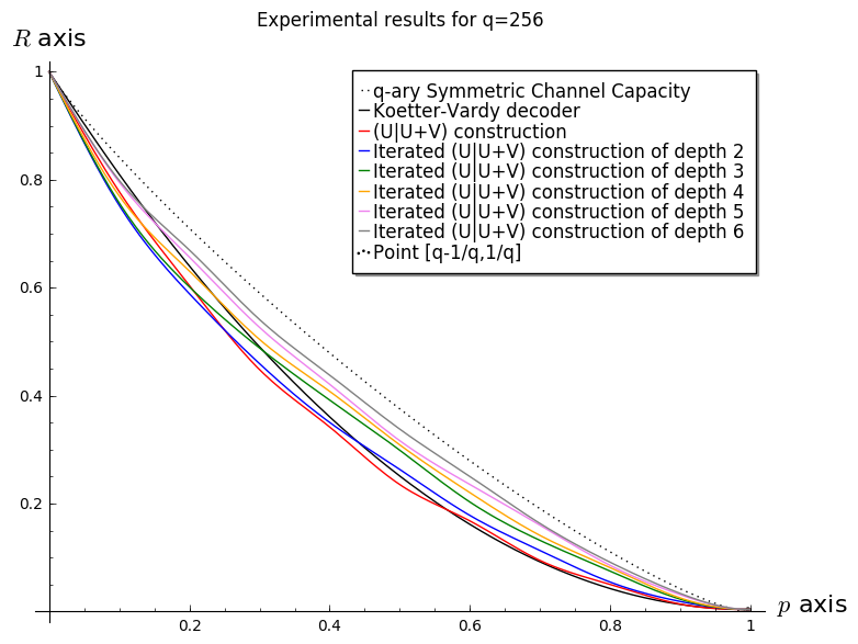
Fig. 5: average Koetter-Vardy capacity plotted against the crossover error probability $p$ for seven code constructions. The noise model is a a ${q\text{-SC}_{p}}$. .

6 Attaining the capacity with an iterated $\left(U\mid U+V\right)$ construction

When the number of levels for which we iterate this construction tends to infinity, we attain the capacity of any $q$-ary symmetric channel at least when the cardinality $q$ is prime. This is a straighforward consequence of the fact that polar codes attain the capacity of any $q$-ary symmetric channel. Moreover the probability of error after decoding can be made to be almost exponentially small with respect to the overall codelength. More precisely the aim of this section is to prove the following results about the probability of error.

Theorem 15.

Let $W$ be a cyclic-symmetric $q$-ary channel where $q$ is prime. Let $C$ be the capacity of this channel. There exists $\epsilon_{0}>0$ such that for any $\epsilon$ in the range $(0,\epsilon_{0})$ and any $\beta$ in the range $(0,1/2)$ there exists a sequence of iterated $\left(U\mid U+V\right)$ codes with Reed-Solomon constituent codes of arbitrarily large length which have rate $\geq C-\epsilon$ when the codelength is sufficiently large and whose probability of error $P_{e}$ is upper bounded by

$$P_{e}\leq ne^{-\frac{K(\epsilon,\beta)N}{n\log N}}$$

when decoded with the iterated $\left(U\mid U+V\right)$ decoder based on decoding the constituent codes with the Koetter-Vardy decoder with listsize bounded by $\mathcal{O}\left(\frac{1}{\epsilon}\right)$ and where $N$ is the codelength, $n=O(\log\log N)^{1/\beta}$, and $K(\epsilon,\beta)$ is some positive function of $\epsilon$ and $\beta$.

For the iterated $\left(U\mid U+V\right)$-construction with algebraic geometry codes as constituent codes we obtain an even stronger result which is

Theorem 16.

Let $W$ be a cyclic-symmetric $q$-ary channel where $q$ is prime. Let $C$ be the capacity of this channel. There exists $\epsilon_{0}>0$ such that for any $\epsilon$ in the range $(0,\epsilon_{0})$ there exists a sequence of iterated $\left(U\mid U+V\right)$ codes of arbitrarily large length with AG defining codes of rate $\geq C-\epsilon$ when the codelength is sufficiently large and whose probability of error $P_{e}$ is upper bounded by

$$P_{e}\leq e^{-K(\epsilon)N}$$

when decoded with the iterated $\left(U\mid U+V\right)$ decoder based on the Koetter-Vardy algorithm with listsize bounded by $\mathcal{O}\left(\frac{1}{\epsilon}\right)$ and where $K$ is some positive function of $\epsilon$.

Remarks:

• In other words the exponent of the error probability is in the first case (that is with Reed-Solomon codes) almost of the form $-\frac{K(\epsilon)N}{\log N(\log\log N)^{2+\epsilon}}$ where $\epsilon$ is an arbitrary positive constant. This is significantly better than the concatenation of polar codes with Reed-Solomon codes (see [BJE10, Th. 1] and also [MELK14] for some more practical variation of this construction) which leads to an exponent of the form $-K(\epsilon)\frac{N}{\log^{27/8}N}$.

• The second case leads to a linear exponent and is therefore optimal up to the dependency in $\epsilon$.

• Both results are heavily based on the fact that when the depth of the construction tends to infinity the channels viewed by the decoders at the leaves of the iterated construction polarize: they have either capacity close to $1$ or close to $0$. This follows from a generalization of Arıkan’s polarization result on binary input channels. This requires $q$ to be prime. However it is possible to change slightly the $\left(U\mid U+V\right)$ structure in order to have polarization for all alphabet sizes. Taking for instance in the case where $q$ is a prime power at each node instead of the $\left(U\mid U+V\right)$ construction a random $(U|U+\alpha V)=\{(\mathbf{u}|\mathbf{u}+\alpha\mathbf{v}):\mathbf{u}\in U,\;\mathbf{v}\in V\}$ where $\alpha$ is chosen randomly in $\mathbb{F}_{q}^{\times}$ would be sufficient here for ensuring polarization of the corresponding channels and would ensure that our results on the probability or error of the iterated construction would also work in this case.

• The reason why these results do not capture the dependency in $\epsilon$ of the exponent comes from the fact that only rather rough results on polarization are used (we rely namely on Theorem 1). Capturing the dependency on $\epsilon$ really needs much more precise results on polarization, such as for instance finite length scaling of polar codes. This will be discussed in the next section.

Overview of the proof of these theorems. The proof of these theorems uses four ingredients.

1. The first ingredient is the polarization theorem 1. It shows that when the number of levels of the recursive $\left(U\mid U+V\right)$ construction tends to infinity, the fraction of the decoders of the constituent codes who face an almost noiseless channel tends to the capacity of the original channel. Here the measure for being noisy is the Bhattacharyya parameter of the channel.

2. We then show that when the Bhattacharyya parameter is close to $0$ the Koetter Vardy capacity of the channel is close to $1$ meaning that we can use Reed-Solomon codes or AG codes of rate close to $1$ for those almost noiseless constituent codes (see Proposition 17).

3. When we use Tsfasman-Vlăduts-Zink AG codes and if $q$ were allowed to be a square prime power, the situation would be really clear. For the codes in our construction that face an almost noiseless channel, we use as constituent AG codes Tsfasman-Vlăduts-Zink AG codes of rate of the form $1-\epsilon-\frac{1}{\sqrt{q}-1}$. This gives an exponentially small (in the length of the constituent code) probability of error for each of those constituent codes by using Theorem 11. For the other codes, we just use the zero code (i.e. the code with only the all-zero codeword). Now in order to get an exponentially small probability of error, it suffices to take the number of levels to be large (but fixed !) so that the fraction of almost noiseless channels is close enough to capacity and to let the length of the constituent codes go to infinity. This gives an exponentially small probability of error when the rate is bounded away from capacity by a term of order $\frac{1}{\sqrt{q}-1}$.

4. In order to get rid of this term, and also in order to be able to use Tsfasman-Vlăduts-Zink AG codes for the case we are interested in, namely an alphabet which is prime, we use another argument. Instead of using a $q$-ary code over a $q$-ary input channel we will use a $q^{m}$-ary code over this $q$-ary input channel. In other words, we are going to group the received symbols by packets of size $m$ and view this as a channel with $q^{m}$-ary input symbols. This changes the Koetter Vardy capacity of the channel. It turns out that the Koetter-Vardy capacity of this new channel is the Koetter-Vardy capacity of the original channel raised to the power $m$ (see Proposition 18). This implies that when the Koetter-Vardy capacity was close to $1-\epsilon$, the new Koetter-Vardy capacity is close to $1-m\epsilon$ and we do not lose much in terms of capacity when moving to a higher alphabet. This allows to use AG codes over a higher alphabet in order to get arbitrarily close to capacity by still keeping an exponentially small probability of error (we can indeed take $m$ fixed but sufficiently large here). For Reed-Solomon codes, the same trick works and allows to use constituent codes of arbitrarily large length by making the alphabet grow with the length of the code. However in this case, we can not take $m$ fixed anymore and this is the reason why we lose a little bit in the behavior of the error exponent. Moreover the number of levels is also increasing in the last case in order to make the Bhattacharyya parameter sufficiently small at the almost noiseless constituent codes so that the Koetter-Vardy stays sufficiently small after grouping symbols together.

Link between the Bhattacharyya parameter and the Koetter-Vardy capacity. We will provide here a proposition showing that for a fixed alphabet size the Koetter Vardy capacity of a channel $W$ is greater than $1-(q-1){\mathcal{Z}\left(W\right)}$. For this purpose, it will be helpful to use an alternate form of the Bhattacharyya parameter

$${\mathcal{Z}\left(W\right)}=\sum_{y\in\mathcal{Y}}\textsf{prob}(Y=y)Z(X|Y=y)$$ (22)

where $X$ is here a uniformly distributed random variable, $Y$ is the output corresponding to sending $X$ over the channel $W$ and

$$Z(X|Y=y)\stackrel{{\scriptstyle\text{def}}}{{=}}\frac{1}{q-1}\sum_{x,x^{\prime}\in\mathbb{F}_{q}\\ x^{\prime}\neq x}\sqrt{\textsf{prob}(X=x|Y=y)}\sqrt{\textsf{prob}(X=x^{\prime}|Y=y)}$$ (23)

Proposition 17.

For a symmetric channel

$$C_{\text{KV}}(W)\geq 1-(q-1){\mathcal{Z}\left(W\right)}$$

Proof.

To simplify formula here we will write $p(x|y)$ for $\textsf{prob}(X=x|Y=y)$, $p(x)$ for $\textsf{prob}(X=x)$ and $p(y)$ for $\textsf{prob}(Y=y)$. The proposition is essentially a consequence of the well known fact that the Rényi entropy which is defined for all $\alpha>0$, $\alpha\neq 1$ by

$$H_{\alpha}(X)\stackrel{{\scriptstyle\text{def}}}{{=}}\frac{1}{1-\alpha}\log_{q}\sum_{x}p(x)^{\alpha}$$

and

$$H_{1}(X)=\lim_{\alpha\rightarrow 1}H_{\alpha}(X)$$

(which turns out to be equal to the usual Shannon entropy taken to the base $q$) is decreasing in $\alpha$. This also holds of course for the “conditional” Rényi entropy which is defined by

$$H_{\alpha}(X|Y=y)\stackrel{{\scriptstyle\text{def}}}{{=}}\frac{1}{1-\alpha}\log_{q}\sum_{x}p(x|y)^{\alpha}$$

Consider now a random variable $X$ which is uniformly distributed over $\mathbb{F}_{q}$ and let $Y$ be the corresponding output of the memoryless channel $W$. By using the definition of the Bhattacharyya parameter given by (22) we can write

$${\mathcal{Z}\left(W\right)}=\sum_{y\in\mathcal{Y}}p(y)Z(X|Y=y)$$

where

$$Z(X|Y=y)=\frac{1}{q-1}\sum_{x,x^{\prime}\in\mathbb{F}_{q},x^{\prime}\neq x}\sqrt{p(x|y)}\sqrt{p(x^{\prime}|y)}$$

We observe that we can relate this quantity to the Rényi entropy of order $\frac{1}{2}$ through

$$H_{1/2}(X|Y=y) = 2\log_{q}\sum_{x}\sqrt{p(x|y)}$$ (24)

$$= \log_{q}\left(\sum_{x}\sqrt{p(x|y)}\sum_{x^{\prime}}\sqrt{p(x^{\prime}|y)}\right)$$

$$= \log_{q}\left(\sum_{x}p(x|y)+\sum_{x,x^{\prime}\in\mathbb{F}_{q},x^{\prime}\neq x}\sqrt{p(x|y)}\sqrt{p(x^{\prime}|y)}\right)$$

$$= \log_{q}\left(1+(q-1)Z(X|Y=y)\right)$$

On the other hand we know that $H_{2}(X|Y=y)\leq H_{1/2}(X|Y=y)$. Recall that

$$H_{2}(X|Y=y)=-\log_{q}\sum_{x}p(x|y)^{2}$$

Using this together with (24) we obtain that

$$-\log_{q}\sum_{x}p(x|y)^{2}\leq\log_{q}\left(1+(q-1)Z(X|Y=y)\right)$$ (25)

Let

$$S\stackrel{{\scriptstyle\text{def}}}{{=}}1-\sum_{x}p(x|y)^{2}$$

Observe that

$$-\log_{q}\sum_{x}p(x|y)^{2}=\log_{q}\left(\frac{1}{\sum_{x}p(x|y)^{2}}\right)=\log_{q}\frac{1}{1-S}\geq\log_{q}(1+S)$$ (26)

Finally by using (25) together with (26) we deduce that $\log_{q}(1+S)\leq\log_{q}\left(1+(q-1)Z(X|Y=y)\right)$ which implies that

$$1-\sum_{x}p(x|y)^{2}=S\leq(q-1)Z(X|Y=y)$$ (27)

By averaging over all $y$’s we get

$$\sum_{y}p(y)\left(1-\sum_{x}p(x|y)^{2}\right)\leq(q-1)\sum_{y}p(y)Z(X|Y=y)$$ (28)

This implies the proposition by noticing that

$$\sum_{y}p(y)\left(1-\sum_{x}p(x|y)^{2}\right) = 1-C_{\text{KV}}$$

$$(q-1)\sum_{y}p(y)Z(X|Y=y) = (q-1){\mathcal{Z}\left(W\right)}.$$

∎

Changing the alphabet. The problem with Reed-Solomon codes is that their length is bounded by their alphabet size. It would be desirable to have more freedom in choosing their length. There is a way to overcome this difficulty by grouping together transmitted symbols into packets and to view each packet as a symbol over a larger alphabet. In other words, assume that we have a memoryless communication channel $W$ with input alphabet $\mathbb{F}_{q}$. Instead of looking for codes defined over $\mathbb{F}_{q}$ we will group input symbols in packets of size $m$ and view them as symbols in the extension field $\mathbb{F}_{q^{m}}$. This will allow us to consider codes defined over $\mathbb{F}_{q^{m}}$ and allows much more freedom in choosing the length of the Reed-Solomon codes components (or more generally the AG components). There is one caveat to this approach, it is that we change the channel model. In such a case the channel is $W^{\otimes m}\stackrel{{\scriptstyle\text{def}}}{{=}}\underbrace{W\otimes W\otimes\dots W}_{m\text{ times}}$ where we define the tensor of two channels by

Definition 6 (Tensor product of two channels).

Let $W$ and $W^{\prime}$ be two memoryless channels with respective input alphabets $\mathcal{X}$ and $\mathcal{X}^{\prime}$ and respective output alphabets $\mathcal{Y}$ and $\mathcal{Y}^{\prime}$. Their tensor product $W\otimes W^{\prime}$ is a memoryless channel with input alphabet $\mathcal{X}\times\mathcal{X}^{\prime}$ and output alphabet $\mathcal{Y}\times\mathcal{Y}^{\prime}$ where the transitions probabilities are given by

$$W\otimes W^{\prime}(y,y^{\prime}|x,x^{\prime})=W(y|x)W(y^{\prime}|x)$$

for all $(x,x^{\prime},y,^{\prime})\in\mathcal{X}\times\mathcal{X}^{\prime}\times\mathcal{Y}\times\mathcal{Y}^{\prime}$.

The Koetter-Vardy capacity of this tensor product is easily related to the Koetter-Vardy capacity of the initial channel through

Proposition 18.

$C_{\text{KV}}(W^{\otimes m})=C_{\text{KV}}(W)^{m}$. If $C_{\text{KV}}(W)=1-\epsilon$ then $C_{\text{KV}}(W^{\otimes m})\geq 1-m\epsilon.$

Proof.

Let $\mathbf{x}=(x_{1}\dots x_{m}\in\mathbb{F}_{q}^{m})$ be the sent symbol for channel $W^{\otimes m}$ and $\mathbf{y}=(y_{1},\dots,y_{m})$ be the received vector. Let $\pi^{m}_{\mathbf{y}}$ be the APP probability vector after receiving $\mathbf{y}$, that is $\pi^{m}_{\mathbf{y}}=(\textsf{prob}(\mathbf{x}=(\alpha_{1},\dots,\alpha_{m})|\mathbf{y})_{(\alpha_{1},\dots,\alpha_{m})\in\mathbb{F}_{q^{m}}}$. We denote the $(\alpha_{1},\dots,\alpha_{m})$ component of this vector by $\pi^{m}_{\mathbf{y}}(\alpha_{1},\dots,\alpha_{m})$. Let $\pi_{y_{i}}=(\textsf{prob}(x_{i}=\alpha|y_{i}))_{\alpha\in\mathbb{F}_{q}}$ be the APP vector for the $i$-th use of the channel. We denote by $\pi_{y_{i}}(\alpha)$ the $\alpha$ component of this vector. Observe that

$$\pi^{m}_{\mathbf{y}}(\alpha_{1}\dots\alpha_{m})=\pi_{y_{1}}(\alpha_{1})\dots\pi_{y_{m}}(\alpha_{m}).$$ (29)

This implies that

$$\left|\!\left|\pi^{m}_{\mathbf{y}}\right|\!\right|^{2}=\left|\!\left|\pi_{y_{1}}\right|\!\right|^{2}\dots\left|\!\left|\pi_{y_{m}}\right|\!\right|^{2}$$

This together with the fact that the channel is memoryless implies that

$$C_{\text{KV}}(W^{\otimes m}) = {\mathbb{E}}\left(\left|\!\left|\pi^{m}_{\mathbf{y}}\right|\!\right|^{2}\right))$$

$$= {\mathbb{E}}\left(\left|\!\left|\pi_{y_{1}}\right|\!\right|^{2}\right)\dots\mathbb{E}\left(\left|\!\left|\pi_{y_{m}}\right|\!\right|^{2}\right)$$

$$= C_{\text{KV}}(W)^{m}$$

The last statement follows easily from this identity and the convexity inequality $(1-x)^{m}\geq 1-mx$ which holds for $x$ in $[0,1]$ and $m\geq 1$. ∎

Proof of Theorem 15. We have now all ingredients at hand for proving Theorem 15. We use Theorem 1 to claim that there exists a lower bound $\ell_{0}$ on the number of levels $\ell$ in a recursive $\left(U\mid U+V\right)$ construction such that

$$\frac{1}{n}\left|i\in\{0,1\}^{\ell}:{\mathcal{Z}\left(W^{i}\right)}\leq 2^{-n^{\beta}}\right|\geq C-\epsilon/2$$ (30)

for all $\ell\geq\ell_{0}$ where $n\stackrel{{\scriptstyle\text{def}}}{{=}}2^{\ell}$. We call the channels that satisfy this condition the good channels. We choose our code to be a recursive $\left(U\mid U+V\right)$-code of depth $\ell$ with Reed-Solomon constituent codes that are of length $q^{m}$ and defined over $\mathbb{F}_{q^{m}}$. The overall length (over $\mathbb{F}_{q}$) of the recursive $\left(U\mid U+V\right)$ code is then

$$N\stackrel{{\scriptstyle\text{def}}}{{=}}2^{\ell}mq^{m}.$$ (31)

The constituent codes $U^{i}$ that face a good channel $W^{i}$ are chosen as Reed-Solomon codes of dimension $k$ given by

$$k=\left\lfloor q^{m}\left(1-m(q-1)2^{-n^{\beta}}-\frac{\epsilon}{4}\right)\right\rfloor$$

whereas all the other codes are chosen to be zero codes. By using Proposition 17 we know that

$$C_{\text{KV}}\left(W^{i}\right)\geq 1-(q-1)2^{-n^{\beta}}.$$

From this we deduce that the Koetter-Vardy of the channel corresponding to grouping together $m$ symbols in $\mathbb{F}_{q}$ has a Koetter-Vardy capacity that satisfies

$$C_{\text{KV}}\left[\left(W^{i}\right)^{\otimes m}\right]\geq 1-m(q-1)2^{-n^{\beta}}.$$

Now we can invoke Theorem 7 and deduce that the probability of error of the Reed-Solomon codes that face these good channels when decoding them with the Koetter-Vardy decoding algorithm with list size bounded by $\mathcal{O}\left(\frac{1}{\epsilon}\right)$ is upper-bounded by a quantity of the form $e^{-Kq^{m}\epsilon^{2}}$. The overall probability of error is bounded by $ne^{-Kq^{m}\epsilon^{2}}$.

We choose now $n$ such that it is the smallest power of two for which the inequality

$$m(q-1)2^{-n^{\beta}}\leq\epsilon/4$$

holds. This implies $n=0(\log^{1/\beta}m)$ as $m$ tends to infinity. Since $\frac{k}{q^{m}}=1-\epsilon/2-o(1)$ as $m$ tends to infinity, the rate of the iterated $\left(U\mid U+V\right)$ code is of order $(C-\epsilon/2)(1-\epsilon/2-o(1))=C-\frac{1+C}{2}\epsilon+\epsilon^{2}/4+o(1)\geq C-\epsilon$ for $\epsilon$ sufficiently small and $n$ sufficiently large when $C<1$. When $C=1$ the theorem is obviously true. This together with the previous upper-bound on the probability of a decoding error imply directly our theorem since $N=nmq^{m}$ and $n=0(\log^{1/\beta}m)$ imply that $m=\frac{\log N(1+o(1))}{\log q}$ as $m$ tends to infinity.

Proof of Theorem 16. Theorem 16 uses similar arguments, the only difference is that now the number of levels $\ell$ in the construction and the parameter $m$ only depend on the gap to capacity we are looking for. We fix $\beta$ to be an arbitrary constant in $(0,1/2)$ and choose $m$ to be the smallest even integer $m$ for which $\frac{1}{\sqrt{q^{m}}-1}$ is smaller than $\epsilon/4$ and the number of levels $\ell$ to be the smallest integer such that we have at the same time

$$\frac{1}{n}\left|i\in\{0,1\}^{\ell}:{\mathcal{Z}\left(W^{i}\right)}\leq 2^{-n^{\beta}}\right| \geq C-\epsilon/4$$

and

$$m(q-1)2^{-n^{\beta}} \leq \epsilon/4$$ (33)

where $n\stackrel{{\scriptstyle\text{def}}}{{=}}2^{\ell}$. Such an $\ell$ necessarily exists by Theorem 1.

We choose our code to be a recursive $\left(U\mid U+V\right)$-code of depth $\ell$ with Tsfasman-Vlăduts-Zink AG constituent codes that are of length $N_{0}$ and defined over $\mathbb{F}_{q^{m}}$. Such codes exist by the Tsfasman-Vlăduts-Zink construction for arbitrarily large lengths because $m$ is even. The overall length (over $\mathbb{F}_{q}$) of the recursive $\left(U\mid U+V\right)$ code is then

$$N\stackrel{{\scriptstyle\text{def}}}{{=}}2^{\ell}mN_{0}.$$ (34)

For the constituent codes $U^{i}$ that face a good channel $W^{i}$, we choose the rate of the AG code to be $\frac{k}{N_{0}}$ where

$$k=\left\lfloor N_{0}(1-m(q-1)2^{-n^{\beta}}-\frac{1}{\sqrt{q^{m}}-1}-\frac{\epsilon}{4})\right\rfloor$$

whereas all the other codes are chosen to be zero codes. The rate of the codes that face a good channel is clearly greater than or equal a quantity of the form $1-3\epsilon/4+o(1)$ as $N_{0}$ goes to infinity by using (33) and $\frac{1}{\sqrt{q^{m}}-1}\leq\epsilon/4$. The overall rate $R$ of the iterated $\left(U\mid U+V\right)$ code satisfies therefore $R\geq(C-\epsilon/4)(1-3\epsilon/4+o(1))\geq C-\frac{3C+1}{4}\epsilon+3\epsilon^{2}/4+o(1)\geq C-\epsilon$ for $\epsilon$ sufficiently small and $N_{0}$ sufficiently large when $C<1$. We can make the assumption $C<1$ from now on, since when $C=1$ the theorem is trivially true.

On the other hand, the error probability of decoding a code $U^{i}$ facing a good channel $W^{i}$ with the Koetter-Vardy decoding algorithm with list size bounded by $\mathcal{O}\left(\frac{1}{\epsilon}\right)$ is upperbounded by a quantity of the form $e^{-KN_{0}\epsilon^{2}}$ by using Theorem 11 since the rate $R_{0}$ of such a code satisfies

$$R_{0} \leq 1-m(q-1)2^{-n^{\beta}}-\frac{1}{\sqrt{q^{m}}-1}-\frac{\epsilon}{4}+o(1)$$

$$\leq C_{\text{KV}}({(W^{i})}^{\otimes m})-\frac{1}{\sqrt{q^{m}}-1}-\frac{\epsilon}{4}+o(1)$$

by using the lower bound on the Koetter-Vardy capacity of a good channel that follows from Propositions 17 and 18. The overall probability of error is therefore bounded by $ne^{-KN_{0}\epsilon^{2}}$. This probability is of the form announced in Theorem 16 since $m$ and $n$ are quantities that only depend on $q$ and $\epsilon$.

7 Conclusion

A variation on polar codes that is much more flexible. We have given here a variation of polar codes that allows to attain capacity with a polynomial-time decoding complexity in a more flexible way than standard polar codes. It consists in taking an iterated-$\left(U\mid U+V\right)$ construction based on Reed-Solomon codes or more generally AG codes. Decoding consists in computing the APP of each position in the same way as polar codes and then to decode the constituent codes with a soft information decoder, the Koetter-Vardy list decoder in our case. Polar codes are indeed a special case of this construction by taking constituent codes that consist of a single symbol. However when we take constituent codes which are longer we benefit from the fact that we do not face a binary alternative as for polar codes, i.e. putting information or not in the symbol depending on the noise model for this symbol, but can choose freely the length (at least in the AG case) and the rate of the constituent code that face this noise model.

An exponentially small probability of error. This allows to control the rate and error probability in a much finer way as for standard polar codes. Indeed the failure probability of polar codes is essentially governed by the error probability of an information symbol of the polar code facing the noisiest channel (among all information symbols). In our case, this error probability can be decreased significantly by choosing a long enough code and a rate below the noise value that our decoder is able to sustain (which is more or less the Koetter-Vardy capacity of the noisy channel in our case). Furthermore, now we can also put information in channels that were not used for sending information in the polar code case. When using Reed-Solomon codes with this approach we obtain a quasi-exponential decay of the error probability which is significantly smaller than for the standard concatenation of an inner polar code with an outer Reed-Solomon code. When we use AG codes we even obtain an exponentially fast decay of the probability of error after decoding.

The whole work raises a certain number of intriguing questions.

Dependency of the error probability with respect to the gap to capacity. Even if the exponential decay with respect to the codelength of the iterated $\left(U\mid U+V\right)$-construction is optimal, the result says nothing about the behavior of the exponent in terms of the gap to capacity. The best we can hope for is a probability of error which behaves as $e^{-K\epsilon^{2}n}$ where $\epsilon$ is the gap to capacity, that is $\epsilon=C-R$, $C$ being the capacity and $R$ the code rate. We may observe that Theorem 7 gives a behavior of this kind with the caveat that $\epsilon$ is not the gap to capacity there but the gap to the Koetter-Vardy capacity. To obtain a better understanding of the behavior of this exponent, we need to have a much finer understanding of the speed of polarization than the one given in Theorem 1. What we really need is indeed a result of the following form

$$\frac{1}{n}\left|i\in\{0,1\}^{\ell}:{\mathcal{Z}\left(W^{i}\right)}\leq\epsilon\right|\geq C-f(\epsilon,\ell)$$ (35)

which expresses the fraction of “$\epsilon$-good” channels in terms of the gap to capacity with sharp estimates for the “gap” function $f(\epsilon,\ell)$. The problem in our case is that our understanding of the speed of polarization is far from being complete. Even for binary input channels, the information we have on the function $f(\epsilon,\ell)$ is only partial as shown by [HAU14, GB14, GX15, MHU16]. A better understanding of the speed of polarization could then be used in order to get a better understanding of the decay of the error probability in terms of the gap to capacity. A tantalizing issue is whether or not we get a better scaling than for polar codes.

Choosing other kernels. The iterated $\left(U\mid U+V\right)$-construction can be viewed as choosing the original polar codes from Arikan associated to the kernel $\boldsymbol{G}=\begin{pmatrix}1&0\\ 1&1\end{pmatrix}$. Taking larger kernels does not improve the error probability after decoding in the binary case for polar codes, unless taking very large kernels as shown in [Kor09], however this is not the case for non binary kernels. Even ternary kernels, such as for instance the ternary “Reed-Solomon” kernel $\boldsymbol{G}_{\text{RS}}=\begin{pmatrix}1&1&0\\ 1&-1&1\\ 1&1&1\end{pmatrix}$ results in a better behavior of the probability of error after decoding (see [MT14]). This raises the issue whether other kernels would allow to obtain better results in our case. In other words, would other generalized concatenated code constructions do better in our case ? Interestingly enough, it is not necessary a Reed-Solomon kernel which gives the best results in our case. Preliminary results seem to show that it should be better to take the kernel $\boldsymbol{G}=\begin{pmatrix}1&0&0\\ 1&1&0\\ 1&1&1\end{pmatrix}$ rather than the aforementioned Reed-Solomon kernel. The last kernel would correspond to a $\left(U\mid U+V\mid U+V+W\right)$ construction which is defined by

$$\left(U\mid U+V\mid U+V+W\right)=\left\{(\mathbf{u}\mid\mathbf{u}+\mathbf{v}\mid\mathbf{u}+\mathbf{v}+\mathbf{w}):\mathbf{u}\in U,\;\mathbf{v}\in V\text{ and }\mathbf{w}\in W\right\}.$$

One level of concatenation outperforms the $\left(U\mid U+V\right)$ construction on the ${q\text{-SC}_{p}}$. In particular it allows to increase the slope at the origin of the “infinite Koetter-Vardy capacity curve” (when compared to the curve for one level in Figure 4). This seems to be the key for choosing good kernels. This issue requires further studies.

Practical constructions. We have explored here the theoretical behavior of this coding/decoding strategy. What is suggested by the experimental evidence shown in Subsection 5.3 is that these codes do not only have some theoretical significance, but that they should also yield interesting codes for practical applications. Indeed Figure 5 shows that it should be possible to get very close to the channel capacity by using only a construction with a small depth, say $5-6$ together with constituent codes of moderate length that can be chosen to be Reed-Solomon codes (say codes of length a hundred/a few hundred at most). This raises many issues that we did not cover here, such as for instance

• to choose appropriately the code rate of each constituent code in order to maximize the overall rate with respect to a certain target error probability;

• choose the multiplicities for each constituent code in order to attain a good overall tradeoff complexity vs. performance;

• choose other constituent codes such as AG codes especially in cases where the channel is an $\mathbb{F}_{q}$-input channel for small values of $q$. It might also be worthwhile to study the use of subfield subcodes of Reed-Solomon codes in this setting (for instance BCH codes).

The whole strategy leads to use Koetter-Vardy decoding for Reed-Solomon/AG codes in a regime where the rate gets either very close to $0$ or to $1$. This could be exploited to lower the complexity of generic Koetter-Vardy decoding.

Appendix notation and assumption

Throughout the appendix we will use the same notation as in Section 2 and denote by $U_{i}$ a constituent code of an iterated $\left(U\mid U+V\right)$ construction of some depth $\ell$. Here $i$ is an $\ell$-bit word. We assume in the appendix that all the constituent codes are Reed-Solomon codes and that the model of error is the $q$-ary symmetric channel of crossover probability $p$ (${q\text{-SC}_{p}}$). We also denote by $\pi_{i}$ the APP probability vectors computed for decoding $U_{i}$. Without loss of generality we may assume that the codeword which is sent is the $0$ codeword. With this assumption, in order to reduce the number of cases to be considered it will be very convenient to give these APP vectors only up to a permutation acting on all positions with the exception of the first one which will always be fixed. We will namely use the following notation.

Notation 19.

For two probability vectors $\mathbf{p}$ and $\mathbf{p}^{\prime}$ in $\mathbb{R}^{q}$ we will write $\mathbf{p}\stackrel{{\scriptstyle\sigma}}{{=}}\mathbf{p}^{\prime}$ if and only if $p(0)=p^{\prime}(0)$ and $p(1),\dots,p(q-1)$ is a permutation of $p^{\prime}(1),\dots,p^{\prime}(q-1)$.

Moreover also in order to simplify the expressions wich will appear in these APP vectors we will use the following notation

Notation 20.

$\varepsilon^{t}$ denotes an arbitrary function of $q$ which satisfies $|\varepsilon^{t}|=\mathcal{O}\left(\frac{1}{q^{t}}\right)$.

Appendix A The $\left(U\mid U+V\right)$ construction

With the zero codeword assumption, the distribution of the APP vector ${\mathbold{\pi}}$ of a ${q\text{-SC}_{p}}$-channel is as follows ${\mathbold{\pi}}=\left(1-p,\frac{p}{q-1},\frac{p}{q-1},\dots,\frac{p}{q-1}\right)$ with probability $1-p$ and ${\mathbold{\pi}}=\left(\frac{p}{q-1},\dots,\frac{p}{q-1},1-p,\frac{p}{q-1},\dots,\frac{p}{q-1}\right)$ with probability $\frac{p}{q-1}$ where the term $1-p$ appears in an arbitrary position with the exception of the first one. We summarize this in Table 1.

Table 1:

${\mathbold{\pi}}$	probability	$\left|\!\left|{\mathbold{\pi}}\right|\!\right|^{2}$
$p_{0}^{0}=\left(1-p,\frac{p}{q-1},\frac{p}{q-1},\dots,\frac{p}{q-1}\right)$	$1-p$	$(1-p)^{2}+\varepsilon$
$p_{0}^{1}\stackrel{{\scriptstyle\sigma}}{{=}}\left(\frac{p}{q-1},1-p,\frac{p}{q-1}\dots\frac{p}{q-1}\right)$	$p$	$(1-p)^{2}+\varepsilon$

The distribution of ${\mathbold{\pi}}\times{\mathbold{\pi}}^{\prime}$ where ${\mathbold{\pi}}$ and ${\mathbold{\pi}}^{\prime}$ are independent and distributed as in Table 1 is given in Table 2.

Table 2:

${\mathbold{\pi}}_{0}$	prob.	$\left|\!\left|{\mathbold{\pi}}\right|\!\right|^{2}$
$\mathbf{p}_{1}^{0}=\left(1-\epsilon,\varepsilon^{2},\dots,\varepsilon^{2}\right)$	$(1-p)^{2}$	$1-\varepsilon$
$\mathbf{p}_{1}^{1}\stackrel{{\scriptstyle\sigma}}{{=}}\left(A,A,B\dots B\right)$	$2p(1-p)$	$\left(\frac{1-p}{2-p}\right)^{2}+\varepsilon$
where $A=\frac{1-p}{2-p}+\varepsilon$ and $B=\frac{p}{(q-1)(2-p)}+\epsilon^{2}$
$\mathbf{p}_{1}^{2}\stackrel{{\scriptstyle\sigma}}{{=}}\left(B,A,A,B\dots B\right)$	$p^{2}+\varepsilon$	$\left(\frac{1-p}{2-p}\right)^{2}+\varepsilon$
with $A$ and $B$ as in the previous case

We have used in Table 2 the following notation.

Lemma 21.

Let ${\mathbold{\pi}}_{0}$ be the APP probability vector viewed by the decoder $U_{0}$. For the channel error model of the code $U_{0}$ we have

$${\mathbb{E}}\left(\left|\!\left|{\mathbold{\pi}}_{0}\right|\!\right|^{2}\right) = \frac{(p+2)(p-1)^{2}}{2-p}+\mathcal{O}\left(\frac{1}{q}\right)$$

The distribution of ${\mathbold{\pi}}\oplus{\mathbold{\pi}}$ where ${\mathbold{\pi}}$ and ${\mathbold{\pi}}^{\prime}$ are independent and distributed as in Table 1 is given in Table 3.

Table 3:

${\mathbold{\pi}}_{1}$	prob.	$\left|\!\left|{\mathbold{\pi}}\right|\!\right|^{2}$
$\mathbf{p}_{1}^{3}=\left(1-p_{1}+\varepsilon,\frac{p_{1}}{q-1}+\varepsilon^{2},\dots,\frac{p_{1}}{q-1}+\varepsilon^{2}\right)$	$(1-p)^{2}$	$(1-p)^{2}+\varepsilon$
where $p_{1}=2p-p^{2}$
$\mathbf{p}_{1}^{4}\stackrel{{\scriptstyle\sigma}}{{=}}\left(\frac{p_{1}}{q-1}+\varepsilon^{2},1-p_{1}+\varepsilon,\frac{p_{1}}{q-1}+\varepsilon^{2}\dots\frac{p_{1}}{q-1}+\varepsilon^{2}\right)$	$2p-p^{2}+\varepsilon$	$(1-p)^{2}+\varepsilon$

Lemma 22.

Let ${\mathbold{\pi}}_{1}$ be the APP probability vector viewed by the decoder $U_{1}$. The channel error model for the code $U_{1}$ is a $q\hbox{-SC}_{p_{1}+\varepsilon}$ with $p_{1}=2p-p^{2}$ and we have

$${\mathbb{E}}\left(\left|\!\left|{\mathbold{\pi}}_{1}\right|\!\right|^{2}\right) =(1-p)^{4}+\mathcal{O}\left(\frac{1}{q}\right).$$

Important remark: Observe that for the distribution of ${\mathbold{\pi}}\times{\mathbold{\pi}}^{\prime}$ and the distribution of ${\mathbold{\pi}}\oplus{\mathbold{\pi}}^{\prime}$ we have implicitly used the fact that with probability $1-\mathcal{O}\left(\frac{1}{q}\right)=1-\epsilon$ the two vectors ${\mathbold{\pi}}$ and ${\mathbold{\pi}}^{\prime}$ have their $1-p$ entry in a different position when ${\mathbold{\pi}}$ and ${\mathbold{\pi}}^{\prime}$ both correspond to the second case of Table 1. This accounts for the $\epsilon$ term in the probability for the third case of Tables 2 and 3. Since we are interested in obtaining the expected values of ${\mathbb{E}}\left(\left|\!\left|{\mathbold{\pi}}_{i}\right|\!\right|^{2}\right)$ only up to $\mathcal{O}\left(\frac{1}{q}\right)$ we can readily ignore the cases when ${\mathbold{\pi}}$ and ${\mathbold{\pi}}^{\prime}$ have ther $1-p$ value at the same position (assuming that this is not the first position). This reasoning will be used repeatedly in the following sections.

Appendix B The iterated $\left(U\mid U+V\right)$ construction of depth $2$

B.1 Computation of ${\mathbb{E}}\left(\left|\!\left|{\mathbold{\pi}}_{00}\right|\!\right|^{2}\right)$

Note that ${\mathbold{\pi}}_{00}={\mathbold{\pi}}\times{\mathbold{\pi}}^{\prime}$ where ${\mathbold{\pi}}$ and ${\mathbold{\pi}}^{\prime}$ are independent and distributed as ${\mathbold{\pi}}_{0}$ which is given in Table 2. Table 4 summarizes this distribution.

Table 4:

${\mathbold{\pi}}_{00}$	prob.	$\left|\!\left|{\mathbold{\pi}}\right|\!\right|^{2}$
$\mathbf{p}_{2}^{0}\stackrel{{\scriptstyle\text{def}}}{{=}}\left\{\begin{array}[]{c}\mathbf{p}_{1}^{0}\times\mathbf{p}_{1}^{0},\mathbf{p}_{1}^{0}\times\mathbf{p}_{1}^{1},\\ \mathbf{p}_{1}^{0}\times\mathbf{p}_{1}^{2},\mathbf{p}_{1}^{1}\times\mathbf{p}_{1}^{1}\end{array}\right\}=\left(1-\epsilon,\varepsilon^{2},\dots,\varepsilon^{2}\right)$	$(1-p)^{2}(1-2p+3p^{3})+\varepsilon$	$1-\varepsilon$
$\mathbf{p}_{2}^{1}\stackrel{{\scriptstyle\text{def}}}{{=}}\mathbf{p}_{1}^{1}\times\mathbf{p}_{1}^{2}\stackrel{{\scriptstyle\sigma}}{{=}}\left(C,C,C,C,D\dots D\right)$	$4p^{2}(1-p)^{2}+\varepsilon$	$4\left(\frac{1-p}{4-3p}\right)^{2}+\varepsilon$
where $C=\frac{1-p}{4-3p}+\varepsilon$ and $D=\frac{p}{(q-1)(4-3p)}+\varepsilon^{2}$
$\mathbf{p}_{2}^{2}\stackrel{{\scriptstyle\text{def}}}{{=}}\mathbf{p}_{1}^{2}\times\mathbf{p}_{1}^{2}\stackrel{{\scriptstyle\sigma}}{{=}}\left(D,C,C,C,C,D\dots D\right)$	$p^{2}+\varepsilon$	$4\left(\frac{1-p}{4-3p}\right)^{2}+\varepsilon$
with $C$ and $D$ as in the previous case

Lemma 23.

Let ${\mathbold{\pi}}_{00}$ be the APP probability vector viewed by the decoder $U_{00}$. For the channel error model of the code $U_{00}$ we have

$${\mathbb{E}}\left(\left|\!\left|{\mathbold{\pi}}_{00}\right|\!\right|^{2}\right) = \frac{(5p^{3}-6p^{2}-5p-4)(1-p)^{2}}{3p-4}+\mathcal{O}\left(\frac{1}{q}\right)$$

B.2 Computation of ${\mathbb{E}}\left(\left|\!\left|{\mathbold{\pi}}_{01}\right|\!\right|^{2}\right)$

It can be observed that ${\mathbold{\pi}}_{01}={\mathbold{\pi}}\oplus{\mathbold{\pi}}^{\prime}$ where ${\mathbold{\pi}}$ and ${\mathbold{\pi}}^{\prime}$ are independent and distributed as ${\mathbold{\pi}}_{0}$ which is given in Table 2. Table 5 summarizes this distribution.

Table 5:

${\mathbold{\pi}}_{01}$	prob.	$\left|\!\left|{\mathbold{\pi}}\right|\!\right|^{2}$
$\mathbf{p}_{2}^{3}\stackrel{{\scriptstyle\text{def}}}{{=}}\mathbf{p}_{1}^{0}\oplus\mathbf{p}_{1}^{0}=\left(1-\epsilon,\varepsilon^{2},\dots,\varepsilon^{2}\right)$	$(1-p)^{4}$	$1-\varepsilon$
$\mathbf{p}_{2}^{4}\stackrel{{\scriptstyle\text{def}}}{{=}}\mathbf{p}_{1}^{0}\oplus\mathbf{p}_{1}^{1}\stackrel{{\scriptstyle\sigma}}{{=}}\left(E,E,F\dots F\right)$	$4p(1-p)^{3}$	$2\left(\frac{1-p}{2-p}\right)^{2}+\varepsilon$
with $E=\frac{1-p}{2-p}+\varepsilon$ and $F=\frac{p}{(2-p)(q-1)}+\varepsilon^{2}$
$\mathbf{p}_{2}^{5}\stackrel{{\scriptstyle\text{def}}}{{=}}\mathbf{p}_{1}^{0}\oplus\mathbf{p}_{1}^{2}\stackrel{{\scriptstyle\sigma}}{{=}}\left(F,E,E,F\dots F\right)$	$2p^{2}(1-p)^{2}+\varepsilon$	$2\left(\frac{1-p}{2-p}\right)^{2}+\varepsilon$
with $E$ and $F$ as in the previous case
$\mathbf{p}_{2}^{6}\stackrel{{\scriptstyle\text{def}}}{{=}}\mathbf{p}_{1}^{1}\oplus\mathbf{p}_{1}^{1}\stackrel{{\scriptstyle\sigma}}{{=}}\left(G,G,G,G,H\dots H\right)$	$4p^{2}(1-p)^{2}+\varepsilon$	$4\left(\tfrac{1-p}{2-p}\right)^{4}+\varepsilon$
where $G=\left(\frac{1-p}{2-p}\right)^{2}+\varepsilon$ and $H=\frac{p(4-3p)}{(q-1)(2-p)^{2}}+\varepsilon^{2}$
$\mathbf{p}_{2}^{7}\stackrel{{\scriptstyle\text{def}}}{{=}}\mathbf{p}_{1}^{1}\oplus\mathbf{p}_{1}^{2}\stackrel{{\scriptstyle\sigma}}{{=}}\left(H,G,G,G,G,H\dots H\right)$	$4p^{2}(1-p)^{2}+p^{2}+\varepsilon$	$4\left(\tfrac{1-p}{2-p}\right)^{4}+\varepsilon$
with $G$ and $H$ as in the previous case

Lemma 24.

Let ${\mathbold{\pi}}_{01}$ be the APP probability vector viewed by the decoder $U_{01}$. For the channel error model of the code $U_{01}$ we have

$${\mathbb{E}}\left(\left|\!\left|{\mathbold{\pi}}_{01}\right|\!\right|^{2}\right) = \frac{(2+p)^{2}(1-p)^{4}}{(2-p)^{2}}+\mathcal{O}\left(\frac{1}{q}\right)$$

B.3 Computation of ${\mathbb{E}}\left(\left|\!\left|{\mathbold{\pi}}_{10}\right|\!\right|^{2}\right)$ and ${\mathbb{E}}\left(\left|\!\left|{\mathbold{\pi}}_{11}\right|\!\right|^{2}\right)$

Note that ${\mathbold{\pi}}_{10}$ and ${\mathbold{\pi}}_{11}$ are distributed like ${\mathbold{\pi}}\times{\mathbold{\pi}}^{\prime}$ and ${\mathbold{\pi}}\oplus{\mathbold{\pi}}^{\prime}$ where ${\mathbold{\pi}}$ and ${\mathbold{\pi}}^{\prime}$ are independent and distributed like ${\mathbold{\pi}}_{1}$ which is itself the APP vector obtained from transmitting $0$ over a $q\hbox{-SC}_{p_{1}+\varepsilon}$ with $p_{1}=2p-p^{2}$. We can therefore use directly both lemmas of the previous section and obtain

Lemma 25.

Let ${\mathbold{\pi}}_{10}$ and ${\mathbold{\pi}}_{11}$ be the APP probability vectors viewed by the decoder $U_{10}$ and $U_{11}$, respectively. For the channel error model of the code $U_{10}$ we have

$${\mathbb{E}}\left(\left|\!\left|{\mathbold{\pi}}_{10}\right|\!\right|^{2}\right) = \frac{(2+p_{1})(1-p_{1})^{2}}{(2-p_{1})}+\mathcal{O}\left(\frac{1}{q}\right)=\frac{(1-p)^{4}(-p^{2}+2p+2)}{(p^{2}-2p+2)}+\mathcal{O}\left(\frac{1}{q}\right)$$

The channel error model for the code $U_{11}$ is a $q\hbox{-SC}_{p_{2}+\varepsilon}$ with $p_{2}=2p_{1}-p_{1}^{2}=p(2-p)(p^{2}-2p+2)$ and we have

$${\mathbb{E}}\left(\left|\!\left|{\mathbold{\pi}}_{11}\right|\!\right|^{2}\right) = (1-p_{2})^{2}+\mathcal{O}\left(\frac{1}{q}\right)=(1-p)^{8}+\mathcal{O}\left(\frac{1}{q}\right)$$

Appendix C The iterated $\left(U\mid U+V\right)$ construction of depth $3$

C.1 Computation of ${\mathbb{E}}\left(\left|\!\left|{\mathbold{\pi}}_{000}\right|\!\right|^{2}\right)$

Note that ${\mathbold{\pi}}_{000}={\mathbold{\pi}}\times{\mathbold{\pi}}^{\prime}$ where ${\mathbold{\pi}}$ and ${\mathbold{\pi}}^{\prime}$ are independent and distributed as ${\mathbold{\pi}}_{00}$ which is given in Table 4. Table 6 summarizes this distribution.

Table 6:

${\mathbold{\pi}}_{000}$	prob.	$\left|\!\left|{\mathbold{\pi}}\right|\!\right|^{2}$
$\mathbf{p}_{3}^{0}=\left\{\begin{array}[]{c}\mathbf{p}_{2}^{0}\times\mathbf{p}_{2}^{0},\mathbf{p}_{2}^{0}\times\mathbf{p}_{2}^{1}\\ \mathbf{p}_{2}^{0}\times\mathbf{p}_{2}^{2},\mathbf{p}_{2}^{1}\times\mathbf{p}_{2}^{1}\end{array}\right\}=\left(1-\varepsilon,\varepsilon^{2},\dots,\varepsilon^{2}\right)$	$1-8p^{7}(1-p)-p^{8}+\varepsilon$	$1-\varepsilon$
$\mathbf{p}_{3}^{1}=\mathbf{p}_{2}^{1}\times\mathbf{p}_{2}^{2}\stackrel{{\scriptstyle\sigma}}{{=}}(\underbrace{I,\ldots,I}_{8\text{-times}},J,\dots,J)$	$8p^{7}(1-p)+\varepsilon$	$8\left(\frac{1-p}{8-7p}\right)^{2}+\varepsilon$
with $I=\frac{1-p}{8-7p}+\varepsilon$ and $J=\frac{p}{(8-7p)(q-1)}+\varepsilon$
$\mathbf{p}_{3}^{2}=\mathbf{p}_{2}^{2}\times\mathbf{p}_{2}^{2}\stackrel{{\scriptstyle\sigma}}{{=}}(J,\underbrace{I,\ldots,I}_{8\text{-times}},J,\dots,J)$	$p^{8}+\varepsilon$	$8\left(\frac{1-p}{8-7p}\right)^{2}+\varepsilon$
with $I$ and $J$ as in the previous case

Lemma 26.

Let ${\mathbold{\pi}}_{000}$ be the APP probability vector viewed by the decoder $U_{000}$ decoder. For the channel error model of the code $U_{000}$ we have

$${\mathbb{E}}\left(\left|\!\left|{\mathbold{\pi}}_{000}\right|\!\right|^{2}\right) = \frac{-(41p^{7}-14p^{6}-13p^{5}-12p^{4}-11p^{3}-10p^{2}-9p-8)(1-p)^{2}}{(8-7p)}+\mathcal{O}\left(\frac{1}{q}\right)$$

C.2 Computation of ${\mathbb{E}}\left(\left|\!\left|{\mathbold{\pi}}_{001}\right|\!\right|^{2}\right)$

It can be observed that ${\mathbold{\pi}}_{001}={\mathbold{\pi}}\oplus{\mathbold{\pi}}^{\prime}$ where ${\mathbold{\pi}}$ and ${\mathbold{\pi}}^{\prime}$ are independent and distributed as ${\mathbold{\pi}}_{00}$ which is given in Table 4. Table 7 summarizes this distribution.

Table 7: It is easy to check that $\left|\!\left|\mathbf{p}_{3}^{3}\right|\!\right|^{2}=1-\varepsilon$, $\left|\!\left|\mathbf{p}_{3}^{4}\right|\!\right|^{2}=4C^{2}+\varepsilon$ and $\left|\!\left|\mathbf{p}_{3}^{5}\right|\!\right|^{2}=16K^{2}+\varepsilon$ with $C$ and $K$ as defined in this table.

${\mathbold{\pi}}_{001}$	prob.	$\left|\!\left|{\mathbold{\pi}}\right|\!\right|^{2}$
$\mathbf{p}_{3}^{3}=\mathbf{p}_{2}^{0}\oplus\mathbf{p}_{2}^{0}\stackrel{{\scriptstyle\sigma}}{{=}}\left(1-\epsilon,\varepsilon^{2},\dots,\varepsilon^{2}\right)$	$(3p^{2}+2p+1)^{2}(1-p)^{4}+\varepsilon$	$1-\varepsilon$
$\mathbf{p}_{3}^{4}=\left\{\begin{array}[]{c}\mathbf{p}_{2}^{0}\oplus\mathbf{p}_{2}^{1},\\ \mathbf{p}_{2}^{0}\oplus\mathbf{p}_{2}^{2}\end{array}\right\}\stackrel{{\scriptstyle\sigma}}{{=}}(\underbrace{C,\ldots,C}_{4\text{-times}},D,\dots,D)$	$2(3p^{2}+2p+1)(4-3p)(1-p)^{2}p^{3}$	$4\left(\frac{1-p}{4-3p}\right)^{2}$
with $C=\frac{1-p}{4-3p}+\varepsilon$ and $D=\frac{p}{(q-1)(4-3p)}+\varepsilon^{2}$	$+\varepsilon$	$+\varepsilon$
$\mathbf{p}_{3}^{5}=\left\{\begin{array}[]{c}\mathbf{p}_{2}^{1}\oplus\mathbf{p}_{2}^{1},\\ \mathbf{p}_{2}^{1}\oplus\mathbf{p}_{2}^{2},\\ \mathbf{p}_{2}^{2}\oplus\mathbf{p}_{2}^{2}\end{array}\right\}\stackrel{{\scriptstyle\sigma}}{{=}}(\underbrace{K,\ldots,K}_{16\text{-times}},L,\dots,L)$	$(3p-4)^{2}p^{6}+\varepsilon$	$16\left(\frac{1-p}{4-3p}\right)^{4}+\varepsilon$
with $K=\left(\frac{1-p}{4-3p}\right)^{2}+\varepsilon$ and $L=\frac{(8-7p)p}{(4-3p)^{2}(q-1)}+\varepsilon^{2}$

Lemma 27.

Let ${\mathbold{\pi}}_{001}$ be the APP probability vector viewed by the decoder $U_{001}$ decoder. For the channel error model of the code $U_{001}$ we have

$${\mathbb{E}}\left(\left|\!\left|{\mathbold{\pi}}_{001}\right|\!\right|^{2}\right) = \frac{\left(5p^{3}-6p^{2}-5p-4\right)^{2}(1-p)^{4}}{(4-3p)^{2}}+\mathcal{O}\left(\frac{1}{q}\right)$$

C.3 Computation of ${\mathbb{E}}\left(\left|\!\left|{\mathbold{\pi}}_{010}\right|\!\right|^{2}\right)$

It can be observed that ${\mathbold{\pi}}_{010}={\mathbold{\pi}}\times{\mathbold{\pi}}^{\prime}$ where ${\mathbold{\pi}}$ and ${\mathbold{\pi}}^{\prime}$ are independent and distributed as ${\mathbold{\pi}}_{01}$ which is given in Table 5. Table 8 summarizes this distribution.

Table 8: It is easy to check that $\left|\!\left|\mathbf{p}_{3}^{6}\right|\!\right|^{2}=1-\varepsilon$, $\left|\!\left|\mathbf{p}_{3}^{7}\right|\!\right|^{2}=4C^{2}+\varepsilon$, $\left|\!\left|\mathbf{p}_{3}^{8}\right|\!\right|^{2}=4M^{2}+4N^{2}+\varepsilon$ and $\left|\!\left|\mathbf{p}_{3}^{9}\right|\!\right|^{2}=8P^{2}+\varepsilon$ with $C$, $M$, $N$ and $P$ as defined in this table.

${\mathbold{\pi}}_{010}$	prob.
$\mathbf{p}_{3}^{6}=\left\{\begin{array}[]{c}\mathbf{p}_{2}^{3}\times\mathbf{p}_{2}^{3},\\ \mathbf{p}_{2}^{3}\times\mathbf{p}_{2}^{4},\\ \mathbf{p}_{2}^{3}\times\mathbf{p}_{2}^{5},\\ \mathbf{p}_{2}^{3}\times\mathbf{p}_{2}^{6},\\ \mathbf{p}_{2}^{3}\times\mathbf{p}_{2}^{7},\\ \mathbf{p}_{2}^{4}\times\mathbf{p}_{2}^{4},\\ \mathbf{p}_{2}^{4}\times\mathbf{p}_{2}^{6},\\ \mathbf{p}_{2}^{6}\times\mathbf{p}_{2}^{6}\end{array}\right\}=\left(1-\epsilon,\varepsilon^{2},\dots,\varepsilon^{2}\right)$	$(1-p)^{4}(1+4p+10p^{2}+4p^{3}-p^{4})+\varepsilon$
$\mathbf{p}_{3}^{7}=\left\{\begin{array}[]{c}\mathbf{p}_{2}^{4}\times\mathbf{p}_{2}^{5},\\ \mathbf{p}_{2}^{5}\times\mathbf{p}_{2}^{5},\end{array}\right\}\stackrel{{\scriptstyle\sigma}}{{=}}(\underbrace{C,\ldots,C}_{4\text{-times}},D,\dots,D)$	$4p^{3}(1-p)^{4}(4-3p)+\varepsilon$
with $C=\frac{1-p}{4-3p}+\varepsilon$ and $D=\frac{p}{(4-3p)(q-1)}+\varepsilon^{2}$
$\mathbf{p}_{3}^{8}=\left\{\begin{array}[]{c}\mathbf{p}_{2}^{4}\times\mathbf{p}_{2}^{7},\\ \mathbf{p}_{2}^{5}\times\mathbf{p}_{2}^{6},\mathbf{p}_{2}^{6}\times\mathbf{p}_{2}^{7},\end{array}\right\}\stackrel{{\scriptstyle\sigma}}{{=}}(M,M,\underbrace{N,\ldots,N}_{4\text{-times}},O,\dots,O)$	$4p^{4}(1-p)^{2}(7p^{2}-18p+12)+\varepsilon$
with $M=\frac{(1-p)^{2}(4-3p)}{7p^{2}-18p+12}+\varepsilon$, $N=\frac{(1-p)^{2}}{7p^{2}-18p+12}+\varepsilon$
and $O=\frac{p(4-3p)}{(7p^{2}-18p+12)(q-1)}+\varepsilon^{2}$
$\mathbf{p}_{3}^{9}=\left\{\begin{array}[]{c}\mathbf{p}_{2}^{6}\times\mathbf{p}_{2}^{7},\\ \mathbf{p}_{2}^{7}\times\mathbf{p}_{2}^{7},\end{array}\right\}\stackrel{{\scriptstyle\sigma}}{{=}}(\underbrace{P,\ldots,P}_{8\text{-times}},Q,\dots,Q)$	$p^{5}(4-3p)(5p^{2}-12p+8)+\varepsilon$
with $P=\frac{(1-p)^{2}}{5p^{2}-12p+8}+\varepsilon$ and $Q=\frac{p(4-3p)}{(5p^{2}-12p+8)(q-1)}+\varepsilon^{2}$

Lemma 28.

Let ${\mathbold{\pi}}_{010}$ be the APP probability vector viewed by the decoder $U_{010}$ decoder. For the channel error model of the code $U_{010}$ we have

$${\mathbb{E}}\left(\left|\!\left|{\mathbold{\pi}}_{010}\right|\!\right|^{2}\right) = \frac{S(p)(1-p)^{4}}{\left(7p^{2}-18p+12\right)\left(5p^{2}-12p+8\right)\left(3p-4\right))}+\mathcal{O}\left(\frac{1}{q}\right)$$

with $S(p)=\left(151p^{9}-662p^{8}+1094p^{7}-1624p^{6}+4105p^{5}-6598p^{4}+4252p^{3}-272p^{2}-96p-384\right)$

C.4 Computation of ${\mathbb{E}}\left(\left|\!\left|{\mathbold{\pi}}_{011}\right|\!\right|^{2}\right)$

It can be observed that ${\mathbold{\pi}}_{011}={\mathbold{\pi}}\oplus{\mathbold{\pi}}^{\prime}$ where ${\mathbold{\pi}}$ and ${\mathbold{\pi}}^{\prime}$ are independent and distributed as ${\mathbold{\pi}}_{01}$ which is given in Table 5. Table 9 summarizes this distribution.

Table 9: It is easy to check that $\left|\!\left|\mathbf{p}_{3}^{10}\right|\!\right|^{2}=1-\varepsilon$, $\left|\!\left|\mathbf{p}_{3}^{11}\right|\!\right|^{2}=\left|\!\left|\mathbf{p}_{3}^{12}\right|\!\right|^{2}=2A^{2}+\varepsilon$, $\left|\!\left|\mathbf{p}_{3}^{13}\right|\!\right|^{2}=4G^{2}+\varepsilon$, $\left|\!\left|\mathbf{p}_{3}^{14}\right|\!\right|^{2}=8R^{2}+\varepsilon$ and $\left|\!\left|\mathbf{p}_{3}^{15}\right|\!\right|^{2}=16T^{2}+\varepsilon$ with $A$, $G$, $R$ and $T$ as defined in this table.

${\mathbold{\pi}}_{011}$	prob.
$\mathbf{p}_{3}^{10}=\mathbf{p}_{2}^{3}\oplus\mathbf{p}_{2}^{3}=\left(1-\epsilon,\varepsilon^{2},\dots,\varepsilon^{2}\right)$	$(1-p)^{8}+\varepsilon$
$\mathbf{p}_{3}^{11}=\mathbf{p}_{2}^{3}\oplus\mathbf{p}_{2}^{4}\stackrel{{\scriptstyle\sigma}}{{=}}\left(A,A,B,\dots,B\right)$	$8p(1-p)^{7}+\varepsilon$
with $A=\frac{1-p}{2-p}+\varepsilon$ and $B=\frac{p}{(2-p)(q-1)}+\varepsilon^{2}$
$\mathbf{p}_{3}^{12}=\mathbf{p}_{2}^{3}\oplus\mathbf{p}_{2}^{5}\stackrel{{\scriptstyle\sigma}}{{=}}\left(B,A,A,B,\dots,B\right)$	$4p^{2}(1-p)^{6}+\varepsilon$
with $A$ and $B$ as in the previous case
$\mathbf{p}_{3}^{13}=\left\{\begin{array}[]{c}\mathbf{p}_{2}^{3}\oplus\mathbf{p}_{2}^{6},\\ \mathbf{p}_{2}^{3}\oplus\mathbf{p}_{2}^{7},\\ \mathbf{p}_{2}^{4}\oplus\mathbf{p}_{2}^{4},\\ \mathbf{p}_{2}^{4}\oplus\mathbf{p}_{2}^{5},\\ \mathbf{p}_{2}^{5}\oplus\mathbf{p}_{2}^{5}\end{array}\right\}\stackrel{{\scriptstyle\sigma}}{{=}}(\underbrace{G,\ldots,G}_{4\text{-times}},H,\dots,H)$	$6(1-p)^{4}(2-p)^{2}p^{2}+\varepsilon$
with $G=\left(\frac{1-p}{2-p}\right)^{2}+\varepsilon$ and $H=\frac{p(4-3p)}{(2-p)^{2}(q-1)}+\varepsilon^{2}$
$\mathbf{p}_{3}^{14}=\left\{\begin{array}[]{c}\mathbf{p}_{2}^{4}\oplus\mathbf{p}_{2}^{6},\\ \mathbf{p}_{2}^{4}\oplus\mathbf{p}_{2}^{7},\\ \mathbf{p}_{2}^{5}\oplus\mathbf{p}_{2}^{6},\\ \mathbf{p}_{2}^{5}\oplus\mathbf{p}_{2}^{7}\end{array}\right\}\stackrel{{\scriptstyle\sigma}}{{=}}(\underbrace{R,\ldots,R}_{8\text{-times}},S,\dots,S)$	$4(1-p)^{2}(2-p)^{3}p^{3}+\varepsilon$
with $R=\left(\frac{1-p}{2-p}\right)^{3}+\varepsilon$ and $S=\frac{(7p^{2}-18p+12)p}{(2-p)^{2}(q-1)}+\varepsilon^{2}$
$\mathbf{p}_{3}^{15}=\left\{\begin{array}[]{c}\mathbf{p}_{2}^{6}\oplus\mathbf{p}_{2}^{6},\\ \mathbf{p}_{2}^{6}\oplus\mathbf{p}_{2}^{7},\\ \mathbf{p}_{2}^{7}\oplus\mathbf{p}_{2}^{7}\end{array}\right\}\stackrel{{\scriptstyle\sigma}}{{=}}(\underbrace{T,\ldots,T}_{16\text{-times}},U,\dots,U)$	$(2-p)^{4}p^{4}+\varepsilon$
with $T=\left(\frac{1-p}{2-p}\right)^{4}+\varepsilon$ and $U=\frac{(5p^{2}-12p+8)p(4-3p)}{(2-p)^{4}(q-1)}+\varepsilon^{2}$

Lemma 29.

Let ${\mathbold{\pi}}_{011}$ be the APP probability vector viewed by the decoder $U_{011}$ decoder. For the channel error model of the code $U_{011}$ we have

$${\mathbb{E}}\left(\left|\!\left|{\mathbold{\pi}}_{010}\right|\!\right|^{2}\right) = \frac{(p+2)^{4}(p-1)^{8}}{(2-p)^{4}}+\mathcal{O}\left(\frac{1}{q}\right)$$

C.5 Computation of ${\mathbb{E}}\left(\left|\!\left|{\mathbold{\pi}}_{100}\right|\!\right|^{2}\right)$, ${\mathbb{E}}\left(\left|\!\left|{\mathbold{\pi}}_{101}\right|\!\right|^{2}\right)$, ${\mathbb{E}}\left(\left|\!\left|{\mathbold{\pi}}_{110}\right|\!\right|^{2}\right)$ and ${\mathbb{E}}\left(\left|\!\left|{\mathbold{\pi}}_{111}\right|\!\right|^{2}\right)$

Note that ${\mathbold{\pi}}_{110}$ and ${\mathbold{\pi}}_{111}$ are distributed like ${\mathbold{\pi}}\times{\mathbold{\pi}}^{\prime}$ and ${\mathbold{\pi}}\oplus{\mathbold{\pi}}^{\prime}$ where ${\mathbold{\pi}}$ and ${\mathbold{\pi}}^{\prime}$ are independent and distributed like ${\mathbold{\pi}}_{11}$ which is itself the APP vector obtained from transmitting $0$ over a $q\hbox{-SC}_{p_{2}+\varepsilon}$ with $p_{2}=2p_{1}-p_{1}^{2}$. We can therefore use directly Lemmas 21 and 22 and obtain

Lemma 30.

Let ${\mathbold{\pi}}_{110}$ and ${\mathbold{\pi}}_{111}$ be the APP probability vectors viewed by the decoder $U_{110}$ and $U_{111}$, respectively. For the channel error model of the code $U_{110}$ we have

$${\mathbb{E}}\left(\left|\!\left|{\mathbold{\pi}}_{110}\right|\!\right|^{2}\right) = \frac{(2+p_{2})(1-p_{2})^{2}}{(2-p_{2})}+\mathcal{O}\left(\frac{1}{q}\right)$$

$$= \frac{-\left(p^{4}-4p^{3}+6p^{2}-4p-2\right)(p-1)^{8}}{(p^{4}-4p^{3}+6p^{2}-4p+2)}+\mathcal{O}\left(\frac{1}{q}\right)$$

The channel error model for the code $U_{111}$ is a $q\hbox{-SC}_{p_{3}+\varepsilon}$ with $p_{3}=2p_{2}-p_{2}^{2}$

$${\mathbb{E}}\left(\left|\!\left|{\mathbold{\pi}}_{111}\right|\!\right|^{2}\right) = (1-p_{3})^{2}+\mathcal{O}\left(\frac{1}{q}\right)=(1-p)^{16}+\mathcal{O}\left(\frac{1}{q}\right)$$

Note that ${\mathbold{\pi}}_{100}$ and ${\mathbold{\pi}}_{101}$ are distributed like ${\mathbold{\pi}}\times{\mathbold{\pi}}^{\prime}$ and ${\mathbold{\pi}}\oplus{\mathbold{\pi}}^{\prime}$ where ${\mathbold{\pi}}$ and ${\mathbold{\pi}}^{\prime}$ are independent and distributed like ${\mathbold{\pi}}_{10}$. We can therefore use directly Lemmas 23 and 24 and obtain

Lemma 31.

Let ${\mathbold{\pi}}_{100}$ and ${\mathbold{\pi}}_{101}$ be the APP probability vectors viewed by the decoder $U_{100}$ and $U_{101}$, respectively. For the channel error model of the code $U_{100}$ and $U_{101}$ we have

$${\mathbb{E}}\left(\left|\!\left|{\mathbold{\pi}}_{100}\right|\!\right|^{2}\right) = \frac{(5p_{1}^{3}-6p_{1}-5p_{1}-4)(1-p_{1})^{2}}{(3p_{1}-4)}+\mathcal{O}\left(\frac{1}{q}\right)$$

$$= \frac{\left(5p^{6}-30p^{5}+66p^{4}-64p^{3}+19p^{2}+10p+4\right)(p-1)^{4}}{(3p^{2}-6p+4)}+\mathcal{O}\left(\frac{1}{q}\right)$$

$${\mathbb{E}}\left(\left|\!\left|{\mathbold{\pi}}_{101}\right|\!\right|^{2}\right) = \frac{(p_{1}+2)^{2}(1-p_{1})^{4}}{(2-p_{1})^{2}}+\mathcal{O}\left(\frac{1}{q}\right)=\frac{(p^{2}-2p-2)^{2}(p-1)^{8}}{(p^{2}-2p+2)^{2}}+\mathcal{O}\left(\frac{1}{q}\right)$$

Appendix D The Koetter-Vardy decoding algorithm for AG codes

The Koetter-Vardy decoding algorithm for Reed-Solomon codes can be adapted to AG codes as was shown in [KV03b]. In this appendix, we give a short description of this algorithm and a review of the main results of [KV03b] that we need to prove Theorem 10. This section is essentially nothing but a subset of results presented for AG codes in the preprint version [KV03b] which we repeat here for the convenience of the reader since the additional material present in the preprint version has not been published as far as we know.

We first begin with the notion of a gap which will be useful to describe the Koetter-Vardy soft decoding algorithm for AG codes. We consider an algebraic curve $\mathcal{X}$ defined over a finite field $\mathbb{F}_{q}$ of genus $g$. Let $Q$ be a rational point on $\mathcal{X}$. We also assume that $\mathcal{X}$ has at least $n$ other rational points $P_{1},\dots,P_{n}$ besides $\mathcal{X}$. A positive integer $i$ is called a (Weierstrass) gap at $Q$ if $\mathcal{L}(iQ)=\mathcal{L}((i-1)Q)$. Otherwise $i$ is a non-gap at $Q$. It is well known that gaps at $Q$ lie in the interval $[0,2g-1]$ and that the number of gaps is equal to $g$.

These gaps at $Q$ can be used to construct a basis for the space $\mathcal{L}(mQ)$: we fix an arbitrary rational function $\phi_{i}\in\mathcal{L}(iQ)\setminus\mathcal{L}((i-1)Q)$ if $i$ is a non-gap at $Q$ and we set $\phi_{i}=0$ otherwise, for $i\in\{0,\ldots,m\}$.

The ring of rational functions that have either no pole or just one pole at $Q$ which is defined by

$$\mathcal{K}_{Q}\stackrel{{\scriptstyle\text{def}}}{{=}}\bigcup_{i=0}^{\infty}\mathcal{L}(iQ)$$

will also be helpful in what follows. In other words, we can write any polynomial $A(Y)\in\mathcal{K}_{Q}[Y]$ in a unique way as $A(Y)=\sum_{i,j}a_{i,j}\phi_{i}Y^{j}$. This allows to define for a pair $(w_{Q},w_{y})$ of nonnegative real numbers the $(w_{Q},w_{y})$-weighted $Q$-valuation of $A(Y)$, denoted by $\deg_{w_{Q},w_{y}}(A(Y))$, which is the maximum over all numbers $iw_{Q}+jw_{y}$ such that $a_{i,j}\neq 0$.

We will also need the notion of the multiplicity of a polynomial in $\mathcal{K}_{Q}[Y]$ at a certain point $P$. For this purpose, it will be convenient to introduce a new basis for $\mathcal{L}(mQ)$. We define $\phi_{0,P},\phi_{1,P},\dots,\phi_{m,P}$ as follows. If there exists at least one $f\in\mathcal{L}(mQ)$ that has multiplicity exactly $i$ at $P$ we set $\phi_{i,P}$ to be one of these functions (we make an arbitrary choice if there are several functions of this kind). If there is no such function we set $\phi_{i,P}=0$. For the case we are interested in, namely $n>m\geq 2g-1$, it is known that there are exactly $g$ indices $i$ for which $\phi_{i,P}=0$. It is known [Sti93] that the set of functions among $\phi_{0,P},\phi_{1,P},\dots,\phi_{m,P}$ which are non zero form a basis of $\mathcal{K}_{Q}[Y]$. We write from now on each $f$ in $\mathcal{L}(mQ)$ in a unique way as

$$f=\sum_{i=0}^{m}a_{i}\phi_{i,P}$$

when we assume that $a_{i}=0$ if $\phi_{i,P}=0$.

Definition 7 (multiplicity of a polynomial in $\mathcal{K}_{Q}[Y]$).

Let $A(Y)$ be a polynomial in $\mathcal{K}_{Q}[Y]$ and consider the shifted polynomial $A(Y+\alpha)$ expressed using the above basis, that is,

$$A(Y+\alpha)=\sum_{i,j}b_{i,j}\phi_{i,P}(Y+\alpha)^{j}$$ (36)

we say that $A(Y)$ has a zero of multiplicity $m$ at the interpolation point $(P,\alpha)$ if $b_{i,j}=0$ for $i+j<m$ and there exists a nonzero coefficient $b_{i,j}$ with $i+j=m$.

We are ready now for describing the Koetter-Vardy decoding algorithm for AG codes. We consider here an AG code $\mathcal{C}_{L}(\mathcal{\mathcal{X}},\mathcal{\mathcal{P}},{mQ})$ of length $n$ over $\mathbb{F}_{q}$ defined by a set of $n+1$ distinct $\mathbb{F}_{q}$-rational points: $Q$ and $\mathcal{P}=\left\{P_{1},\ldots,P_{n}\right\}$. We are also given a multiplicity matrix $\boldsymbol{M}=\left(m_{\alpha,j}\right)_{\begin{subarray}{c}\alpha\in\mathbb{F}_{q}\\ 1\leq j\leq n\end{subarray}}$.

Interpolation step: It consists in computing the (nontrivial) polynomial $Q_{\boldsymbol{M}}(Y)\in\mathcal{K}_{Q}[Y]$ of minimal $(1,m)$-weighted $Q$-valuation that has a zero of multiplicity at least $m_{\alpha,j}$ at the interpolation point $(P_{j},\alpha)$.

Factorization step: It consists in identifying all the factors of $Q_{\boldsymbol{M}}(Y)$ of type $Y-f$ with $f\in\mathcal{L}(mQ)$. The output of the algorithm is a list of the codewords that correspond to these factors.

The following quantities will be useful for understanding this algorithm.

• The number of monomials whose $(w_{Q},w_{y})$-weighted $Q$-valuation is at most $\delta$ is denoted $N_{w_{Q},w_{y}}(\delta,\mathcal{X})$. Thus:

  $$N_{w_{Q},w_{y}}(\delta,\mathcal{X})\stackrel{{\scriptstyle\text{def}}}{{=}}|\left\{(i,j)\mid i,j\geq 0,\text{ $\phi_{i}\neq 0$ and $iw_{Q}+jw_{y}\leq\delta$}\right\}|$$

• We define the inverse function

  $$\Delta_{w_{Q},w_{y}}(\nu,\mathcal{X})\stackrel{{\scriptstyle\text{def}}}{{=}}\min\left\{\delta\in\mathbb{Z}\mid N_{w_{Q},w_{y}}(\delta,\mathcal{X})>\nu\right\}$$

To get a better understanding of the soft-decision algorithm of AG codes the following theorem will be very helpful

Theorem 32 (Theorem 18 and Corollary 20 [KV03b]).

Let $C=C(\boldsymbol{M})$ denote the cost of the multiplicity matrix $\boldsymbol{M}$. The list obtained by factoring the interpolation polynomial $Q_{\boldsymbol{M}}(Y)$ contains a codeword $\mathbf{c}\in\mathcal{C}_{L}(\mathcal{\mathcal{X}},\mathcal{\mathcal{P}},{mQ})$ if

$$\left\langle\boldsymbol{M},\left\lfloor\mathbf{c}\right\rfloor\right\rangle>\Delta_{1,m}(C,\mathcal{X})$$ (37)

We have the following upper bound on $\Delta_{1,m}(C,\mathcal{X})$:

$$\Delta_{1,m}(C,\mathcal{X})\leq g+\sqrt{2m(C+g)+g^{2}}.$$ (38)

Proof.

We first prove that if the condition (37) holds then the list contains the codeword $\mathbf{c}$.

Recall that for every $\mathbf{c}\in\mathcal{C}_{L}(\mathcal{\mathcal{X}},\mathcal{\mathcal{P}},{mQ})$ there exists a rational function $f\in\mathcal{L}(mQ)$ such that $c_{j}=f(P_{j})$ for $j=1,\ldots,n$. Given the interpolation polynomial $Q_{\boldsymbol{M}}(Y)\in\mathcal{K}_{Q}[Y]$, we consider the function $h\in\mathcal{K}_{Q}$ defined by $h=Q_{\boldsymbol{M}}(f)$. By construction, $Q_{\boldsymbol{M}}(Y)$ passes trough the points $(P_{\ell},c_{\ell})$ with multiplicities at least $m_{\ell}$ where $\left\langle\boldsymbol{M},\lfloor\mathbf{c}\rfloor\right\rangle=m_{1}+\cdots+m_{n}$. Then:

• We claim that the function $h=Q_{\boldsymbol{M}}(f)$ has at least $\left\langle\boldsymbol{M},\lfloor\mathbf{c}\rfloor\right\rangle$ zeros in $\mathcal{P}$ counted with multiplicities. Indeed, if $Q_{\boldsymbol{M}}(Y)$ passes through the interpolation point $(P_{\ell},c_{\ell})$ with multiplicity at least $m_{\ell}$ and we express $Q_{\boldsymbol{M}}(Y)$ in the basis of the $\Phi_{i,P_{\ell}}$’s we have

  $$Q_{\boldsymbol{M}}(Y)=\sum_{i,j}a_{i,j}\phi_{i,P_{\ell}}(Y-c_{\ell})^{j}.$$

  But, by (36) it is required that $a_{i,j}=0$ if $i+j<m_{\ell}$. We thus get that $h=Q_{\boldsymbol{M}}(f)=\sum_{i,j}a_{i,j}\phi_{i,P_{\ell}}(f-c_{e}ll)^{j}$ has a zero of multiplicity $m_{\ell}$ at the point $P_{\ell}$ since $f(P_{\ell})=c_{\ell}$.

• Since $f\in\mathcal{L}(mQ)$ and $\deg_{1,m}(Q_{\boldsymbol{M}}(Y))\leq\Delta_{1,m}(C,\mathcal{X})$ then $h$ has at most $\Delta_{1,m}(C,\mathcal{X})$ poles at $Q$. And these are its only poles since $h\in\mathcal{K}_{Q}$.

That is, if $\left\langle\boldsymbol{M},\lfloor\mathbf{c}\rfloor\right\rangle>\Delta_{1,m}(C,\mathcal{X})$, then $h$ has more zeros than poles. Thus, $Q_{\boldsymbol{M}}(f)=h\equiv 0$, in other words, $Y-f$ is a factor of $Q_{\boldsymbol{M}}(Y)$.

For the second statement of the theorem, let $A(X,Y)=\sum_{i=1}^{\infty}\sum_{j=1}^{\infty}a_{i,j}X^{i}Y^{j}$ be a bivariate polynomial over $\mathbb{F}_{q}$ and let $w_{X},w_{Y}\in\mathbb{R}$. In [KV03a], the $(w_{X},w_{Y})$-weighted degree of $A(X,Y)$ is defined as the maximum over all numbers $iw_{X}+jw_{Y}$ such that $a_{i,j}\neq 0$. Moreover, the number of monomials of $(w_{X},w_{Y})$-weighted degree at most $\delta$ is denoted in [KV03a] as $N_{w_{X},w_{Y}}(\delta)$. That is,

$$N_{w_{X},w_{Y}}(\delta)\stackrel{{\scriptstyle\text{def}}}{{=}}\left|\left\{X^{i}Y^{j}\mid i,j\geq 0\hbox{ and }iw_{X}+jw_{Y}\leq\delta\right\}\right|$$

It is easy to see that

$$N_{w_{Q},w_{Y}}(\delta,\mathcal{X})\geq N_{w_{Q},w_{Y}}(\delta)-g\left\lfloor\frac{\delta}{w_{Q}}+1\right\rfloor$$

Indeed, the number of different expressions $\phi_{i}Y^{j}$ in $N_{w_{Q},w_{Y}}(\delta,\mathcal{X})$ is equal to $N_{w_{Q},w_{Y}}(\delta)$ but taking into account that some of the functions $\phi_{i}$ are zero. Then, the result follows from the fact that the number of functions $\phi_{i}$ that are zero, or equivalent, the number of gaps, is bounded by the genus $g$ of the curve $\mathcal{X}$; and the fact that the number of monomials $Y^{j}$ such that $jw_{Q}\leq\delta$ is upper bounded by $\frac{\delta}{w_{Q}}$.

Thus, using [KV03a, Lemma1] we have

$$N_{1,m}(\delta,\mathcal{X})\geq N_{1,m}(\delta)-g\left\lfloor\frac{\delta}{m}+1\right\rfloor>\frac{\delta^{2}}{2m}-g\left(\frac{\delta}{m}+1\right)$$

By replacing $N_{1,m}(\delta,\mathcal{X})$ by $\nu$ we can write the above expression as: $(\delta-g)^{2}<2m(\nu+g)+g^{2}$. Then, by the definition of $\Delta_{1,m}(\nu,\mathcal{X})$, we get the following upper bound:

$$\Delta_{1,m}(\nu,\mathcal{X})\leq g+\sqrt{2m(\nu+g)+g^{2}}$$

∎

As for Reed-Solomon codes we can obtain an algebraic soft-decoding for AG codes with list size limited to $L$. In the following we adapt the ideas of [KV03a] to AG codes.

Lemma 33.

The number of codewords on the list produced by the soft-decision decoder for the AG code $\mathcal{C}_{L}(\mathcal{\mathcal{X}},\mathcal{\mathcal{P}},{mQ})$ with a given multiplicity matrix $\boldsymbol{M}$ does not exceed

$$L_{m}(\boldsymbol{M})\stackrel{{\scriptstyle\text{def}}}{{=}}\frac{g+\sqrt{2m(C+g)+g^{2}}}{m}$$

where $g$ denotes the genus of the curve $\mathcal{X}$ and $C=C(\boldsymbol{M})$ the cost of matrix $\boldsymbol{M}$.

Proof.

Similar to [KV03a, Lemma 15] the number of codewords of the list is upper-bounded by the $(0,1)$-weight $Q$-valuation of the interpolation polynomial $Q_{\boldsymbol{M}}(Y)$. By definition of weighted $Q$-valuation, we have:

$$\deg_{0,1}Q_{\boldsymbol{M}}(Y)\leq\frac{\deg_{1,m}Q_{\boldsymbol{M}}(Y)}{m}\leq\frac{\Delta_{1,m}(C,\mathcal{X})}{m}\leq\frac{g+\sqrt{2m(C+g)+g^{2}}}{m}$$

where the first inequality follows from the definition of weighted $Q$-valuation, the second inequality follows from the definition of $\Delta_{1,m}(C,\mathcal{X})$ and the third inequality follows from Theorem 32. ∎

Remark 4.

The very definition of $L_{m}(\boldsymbol{M})$ implies

$$2C(\boldsymbol{M})=mL_{m}(\boldsymbol{M})^{2}-2L_{m}(\boldsymbol{M})g-2g$$ (39)

Lemma 34.

For a given multiplicity matrix $\boldsymbol{M}$, the algebraic soft-decision decoding algorithm outputs a list that contains a codeword $\mathbf{c}\in\mathcal{C}_{L}(\mathcal{\mathcal{X}},\mathcal{\mathcal{P}},{mQ})$ if

$$\frac{\left\langle\boldsymbol{M},\left\lfloor\mathbf{c}\right\rfloor\right\rangle}{\sqrt{\left\langle\boldsymbol{M},\boldsymbol{M}\right\rangle+\left\langle\boldsymbol{M},1\right\rangle}}\geq\sqrt{m}+\frac{2g+\sqrt{2mg}}{\sqrt{2C(\boldsymbol{M})}}$$

where $g$ denotes the genus of the curve $\mathcal{X}$ and $C=C(\boldsymbol{M})$ the cost of matrix $\boldsymbol{M}$.

Proof.

This follows immediately from Theorem 32 and the fact that

$$\sqrt{2mC}+\sqrt{2mg}+2g\geq g+\sqrt{2m(C+g)+g^{2}}\hbox{ for all }g,m,C\geq 0$$

∎

Let $\boldsymbol{\Pi}$ be a given reliability matrix and $\boldsymbol{M}$ be the corresponding multiplicity matrix produced by [KV03a][Algorithm A]. Then, by [KV03a][Lemma 16] there exists a positive real number $\lambda$ such that $\boldsymbol{M}=\lambda\boldsymbol{\Pi}-\boldsymbol{J}$ where $\boldsymbol{J}$ denotes a $q\times n$ matrix whose entries are all nonnegative real numbers not exceeding $1$. Then:

$$\left\langle\boldsymbol{M},\boldsymbol{M}\right\rangle+\left\langle\boldsymbol{M},\boldsymbol{1}\right\rangle=\lambda^{2}\left\langle\boldsymbol{\Pi},\boldsymbol{\Pi}\right\rangle-\lambda\left\langle\boldsymbol{\Pi},2\boldsymbol{J}-\boldsymbol{1}\right\rangle+\left\langle\boldsymbol{J},\boldsymbol{J}-\boldsymbol{1}\right\rangle$$

By definition we have that

$$\left\langle\boldsymbol{M},\boldsymbol{M}\right\rangle+\left\langle\boldsymbol{M},\boldsymbol{1}\right\rangle=2C(\boldsymbol{M})$$ (40)

We can use both expressions to get a quadratic equation in $\lambda$ which has only one positive root:

$$\lambda=\underbrace{\frac{\left\langle\boldsymbol{\Pi},2\boldsymbol{J}-\boldsymbol{1}\right\rangle}{2\left\langle\boldsymbol{\Pi},\boldsymbol{\Pi}\right\rangle}}_{\lambda_{2}}+\underbrace{\sqrt{\frac{\left\langle\boldsymbol{\Pi},2\boldsymbol{J}-\boldsymbol{1}\right\rangle^{2}}{4\left\langle\boldsymbol{\Pi},\boldsymbol{\Pi}\right\rangle^{2}}+\frac{\left\langle\boldsymbol{J},\boldsymbol{1}-\boldsymbol{J}\right\rangle}{\left\langle\boldsymbol{\Pi},\boldsymbol{\Pi}\right\rangle}+\frac{2C(\boldsymbol{M})}{\left\langle\boldsymbol{\Pi},\boldsymbol{\Pi}\right\rangle}}}_{\lambda_{1}}$$ (41)

D.1 Proof of Theorem 10

By using $\boldsymbol{M}=\lambda\boldsymbol{\Pi}-\boldsymbol{J}$, we can reformulate the sufficient condition of Theorem 34, by rewriting $\left\langle\boldsymbol{M},\lfloor\mathbf{c}\rfloor\right\rangle=\left\langle\lambda\boldsymbol{\Pi}-\boldsymbol{J},\lfloor\mathbf{c}\rfloor\right\rangle=\lambda\left\langle\boldsymbol{\Pi},\lfloor\mathbf{c}\rfloor\right\rangle-\left\langle\boldsymbol{J},\lfloor\mathbf{c}\rfloor\right\rangle$ and obtain

$$\frac{\lambda\left\langle\boldsymbol{\Pi},\lfloor\mathbf{c}\rfloor\right\rangle-\left\langle\boldsymbol{J},\lfloor\mathbf{c}\rfloor\right\rangle}{\sqrt{2C(\boldsymbol{M})}}\geq\sqrt{m}+\frac{g+\sqrt{2mg}}{\sqrt{2C(\boldsymbol{M})}}$$

which is equivalent to

$$\frac{\left\langle\boldsymbol{\Pi},\lfloor\mathbf{c}\rfloor\right\rangle}{\sqrt{\left\langle\boldsymbol{\Pi},\boldsymbol{\Pi}\right\rangle}}\left(\lambda-\frac{\left\langle\boldsymbol{J},\lfloor\mathbf{c}\rfloor\right\rangle}{\left\langle\boldsymbol{\Pi},\lfloor\mathbf{c}\rfloor\right\rangle}\right)\frac{\sqrt{\left\langle\boldsymbol{\Pi},\boldsymbol{\Pi}\right\rangle}}{\sqrt{2C(\boldsymbol{M})}}\geq\sqrt{m}+\frac{g+\sqrt{2mg}}{\sqrt{2C(\boldsymbol{M})}}$$

Using the expression for $\lambda$ in Equation (41), we can express the previous formula as:

$$\frac{\left\langle\boldsymbol{\Pi},\lfloor\mathbf{c}\rfloor\right\rangle}{\sqrt{\left\langle\boldsymbol{\Pi},\boldsymbol{\Pi}\right\rangle}}(F_{1}-F_{2}-F_{3})\geq\sqrt{m}+\frac{g+\sqrt{2mg}}{\sqrt{2C(\boldsymbol{M})}}$$ (42)

with:

$$F_{1} \stackrel{{\scriptstyle\text{def}}}{{=}} \lambda_{1}\frac{\sqrt{\left\langle\boldsymbol{\Pi},\boldsymbol{\Pi}\right\rangle}}{\sqrt{2C(\boldsymbol{M})}}$$

$$= \sqrt{\frac{\left\langle\boldsymbol{\Pi},2\boldsymbol{J}-\boldsymbol{1}\right\rangle^{2}}{4\left\langle\boldsymbol{\Pi},\boldsymbol{\Pi}\right\rangle^{2}}+\frac{\left\langle\boldsymbol{J},\boldsymbol{1}-\boldsymbol{J}\right\rangle}{\left\langle\boldsymbol{\Pi},\boldsymbol{\Pi}\right\rangle}+\frac{2C(\boldsymbol{M})}{\left\langle\boldsymbol{\Pi},\boldsymbol{\Pi}\right\rangle}}\frac{\sqrt{\left\langle\boldsymbol{\Pi},\boldsymbol{\Pi}\right\rangle}}{\sqrt{2C(\boldsymbol{M})}}$$

$$= \sqrt{1+\frac{\left\langle\boldsymbol{J},\boldsymbol{1}-\boldsymbol{J}\right\rangle}{2C(\boldsymbol{M})}+\frac{\left\langle\boldsymbol{\Pi},2\boldsymbol{J}-\boldsymbol{1}\right\rangle^{2}}{8C(\boldsymbol{M})\left\langle\boldsymbol{\Pi},\boldsymbol{\Pi}\right\rangle}}$$

$$\geq 1$$

$$F_{2}\stackrel{{\scriptstyle\text{def}}}{{=}}-\lambda_{2}\frac{\sqrt{\left\langle\boldsymbol{\Pi},\boldsymbol{\Pi}\right\rangle}}{\sqrt{2C(\boldsymbol{M})}}=\frac{1}{\sqrt{2C(\boldsymbol{M})}}\frac{\left\langle\boldsymbol{\Pi},\boldsymbol{1}-2\boldsymbol{J}\right\rangle}{2\sqrt{\left\langle\boldsymbol{\Pi},\boldsymbol{\Pi}\right\rangle}}\leq\frac{1}{\sqrt{2C(\boldsymbol{M})}}\frac{n}{2\sqrt{\tfrac{n}{q}}}$$

To obtain the previous inequality we have used the fact that $\left\langle\boldsymbol{\Pi},\boldsymbol{1}-2\boldsymbol{J}\right\rangle\leq\left\langle\boldsymbol{\Pi},\boldsymbol{1}\right\rangle=n$ and $\left\langle\boldsymbol{\Pi},\boldsymbol{\Pi}\right\rangle\geq\frac{n}{q}$.

$$F_{3}\stackrel{{\scriptstyle\text{def}}}{{=}}\frac{\left\langle\boldsymbol{J},\lfloor\mathbf{c}\rfloor\right\rangle}{\left\langle\boldsymbol{\Pi},\lfloor\mathbf{c}\rfloor\right\rangle}\frac{\sqrt{\left\langle\boldsymbol{\Pi},\boldsymbol{\Pi}\right\rangle}}{\sqrt{2C(\boldsymbol{M})}}\leq\frac{1}{\sqrt{2C(\boldsymbol{M})}}\frac{n}{\sqrt{m}+\frac{g+\sqrt{2mg}}{\sqrt{2C(\boldsymbol{M})}}}=\frac{n}{\sqrt{2C(\boldsymbol{M})m}+g+\sqrt{2mg}}\leq\frac{1}{\sqrt{2C(\boldsymbol{M})}}\frac{n}{\sqrt{m}}$$

To obtain the previous inequality we have made use of the following two observations:

• $\left\langle\boldsymbol{J},\lfloor\mathbf{c}\rfloor\right\rangle\leq\left\langle\boldsymbol{1},\lfloor\mathbf{c}\rfloor\right\rangle=n$;

• if $\boldsymbol{\Pi}$ and $\mathbf{c}$ are such that (19) holds, then a fortiori:

  $$\frac{\left\langle\boldsymbol{\Pi},\lfloor\mathbf{c}\rfloor\right\rangle}{\sqrt{\left\langle\boldsymbol{\Pi},\boldsymbol{\Pi}\right\rangle}}\geq\sqrt{m}+\frac{2g+\sqrt{2mg}}{\sqrt{2C(\boldsymbol{M})}}$$

Using all the bounds that we have just given for the $F_{i}$’s we obtain that (42) holds when

$$\frac{\left\langle\boldsymbol{\Pi},\lfloor\mathbf{c}\rfloor\right\rangle}{\sqrt{\left\langle\boldsymbol{\Pi},\boldsymbol{\Pi}\right\rangle}}\left(1-\frac{1}{\sqrt{2C(\boldsymbol{M})}}\frac{n}{2\sqrt{\tfrac{n}{q}}}-\frac{1}{\sqrt{2C(\boldsymbol{M})}}\frac{n}{\sqrt{m}}\right)\geq\sqrt{m}+\frac{g+\sqrt{2mg}}{\sqrt{2C(\boldsymbol{M})}}$$

which is equivalent to

$$\frac{\left\langle\boldsymbol{\Pi},\lfloor\mathbf{c}\rfloor\right\rangle}{\sqrt{\left\langle\boldsymbol{\Pi},\boldsymbol{\Pi}\right\rangle}}\geq\frac{\sqrt{m}+\frac{g+\sqrt{2mg}}{\sqrt{2C(\boldsymbol{M})}}}{1-\frac{1}{\sqrt{2C(\boldsymbol{M})}}\frac{n}{2\sqrt{\tfrac{n}{q}}}-\frac{1}{\sqrt{2C(\boldsymbol{M})}}\frac{n}{\sqrt{m}}}$$ (43)

From $L\leq L_{m}(\boldsymbol{M})\leq L+1$ and $2C(\boldsymbol{M})=mL_{m}^{2}(\boldsymbol{M})-2L_{m}(\boldsymbol{M})g-2g$ we deduce that

$$\sqrt{2C(\boldsymbol{M})}\geq\sqrt{mL^{2}-2(L+1)g-2g}=L\sqrt{m}\sqrt{1-\tfrac{2g}{mL}\left(1+\tfrac{2}{L}\right)}$$ (44)

Therefore (43) holds if we have

$$\frac{\left\langle\boldsymbol{\Pi},\lfloor\mathbf{c}\rfloor\right\rangle}{\sqrt{\left\langle\boldsymbol{\Pi},\boldsymbol{\Pi}\right\rangle}}\geq\frac{\sqrt{m}+\frac{g+\sqrt{2mg}}{L\sqrt{m}\sqrt{1-\tfrac{2g}{mL}\left(1+\tfrac{2}{L}\right)}}}{1-\frac{1}{L\sqrt{m}\sqrt{1-\tfrac{2g}{mL}\left(1+\tfrac{2}{L}\right)}}\left(\frac{n}{2\sqrt{\tfrac{n}{q}}}+\frac{n}{\sqrt{m}}\right)}$$

By introducing $\tilde{R}=\frac{m}{n}$ and $\tilde{\gamma}\stackrel{{\scriptstyle\text{def}}}{{=}}\frac{g}{m}$ we obtain that this inequality can be rewritten as

$$\frac{\left\langle\boldsymbol{\Pi},\lfloor\mathbf{c}\rfloor\right\rangle}{\sqrt{\left\langle\boldsymbol{\Pi},\boldsymbol{\Pi}\right\rangle}}\geq\sqrt{m}\frac{1+\frac{\tilde{\gamma}+\sqrt{2\tilde{\gamma}}}{L\sqrt{1-\tfrac{2\tilde{\gamma}}{L}\left(1+\tfrac{2}{L}\right)}}}{1-\frac{1}{L\sqrt{1-\tfrac{2\tilde{\gamma}}{L}\left(1+\tfrac{2}{L}\right)}}\left(\frac{\sqrt{q}}{2\sqrt{\tilde{R}}}+\frac{1}{\tilde{R}}\right)}=\sqrt{m}\left(1+\mathcal{O}\left(\frac{1}{L}\right)\right)$$

This completes the proof of the theorem, that is, $\mathbf{c}\in\mathcal{C}_{L}(\mathcal{\mathcal{X}},\mathcal{\mathcal{P}},{mQ})$ is on the list produced by the soft-decision decoder, provided that this last inequality is satisfied.

References

- [Arı09] Erdal Arıkan. Channel polarization: a method for constructing capacity-achieving codes for symmetric binary-input memoryless channels. IEEE Trans. Inform. Theory, 55(7):3051–3073, 2009.
- [BB06] Amir Bennatan and Davis Burshtein. Design and analysis of nonbinary LDPC codes over arbitrary discrete-memoryless channels. IEEE Trans. Inform. Theory, 52(2):549–583, February 2006.
- [BJE10] Mayank Bakshi, Sidharth Jaggi, and Michelle Effros. Concatenated polar codes. In Proc. IEEE Int. Symposium Inf. Theory - ISIT 2010, pages 918–922, Austin, Texas, USA, June 2010. IEEE.
- [DS06] Ilya Dumer and Kirill Shabunov. Soft-decision decoding of Reed-Muller codes: recursive lists. IEEE Trans. Inform. Theory, 52(3):1260–1266, 2006.
- [Dum06] Ilya Dumer. Soft-decision decoding of Reed-Muller codes: a simplified algorithm. IEEE Trans. Inform. Theory, 52(3):954–963, 2006.
- [Gal68] Robert G. Gallager. Information theory and reliable communication, volume 2. Springer, 1968.
- [GB14] Dina Goldin and David Burshtein. Improved bounds on the finite length scaling of polar codes. IEEE Trans. Inform. Theory, 60(11):6966–6978, November 2014.
- [GR06] Venkatesan Guruswami and Atri Rudra. Explicit capacity-achieving list-decodable codes. In Proceedings of the Thirty-eighth Annual ACM Symposium on Theory of Computing, STOC ’06, pages 1–10, New York, NY, USA, 2006. ACM.
- [GS99] Venkatesan Guruswami and Madhu Sudan. Improved decoding of Reed-Solomon and algebraic-geometry codes. IEEE Trans. Inform. Theory, 45(6):1757–1767, 1999.
- [GX15] Venkatesan Guruswami and Patrick Xia. Polar codes: speed of polarization and polynomial gap to capacity. IEEE Trans. Inform. Theory, 61(1):3–16, January 2015.
- [HAU14] S. H. Hassani, K. Alishahi, and Ruediger Urbanke. Finite-length scaling for polar codes. IEEE Trans. Inform. Theory, 60(10):5875–5898, October 2014.
- [Kor09] Satish Babu Korada. Polar Codes for Channel and Source Coding. PhD thesis, ’Ecole Polytechnique Fédérale de Lausanne (EPFL), July 2009.
- [KV03a] Ralf Koetter and Alexander Vardy. Algebraic soft-decision decoding of Reed-Solomon codes. IEEE Trans. Inform. Theory, 49(11):2809–2825, 2003.
- [KV03b] Ralf Koetter and Alexander Vardy. Algebraic soft-decision decoding of Reed-Solomon codes. preprint (long version) of the journal paper of the same name, 2003.
- [MELK14] Hessam Mahdavifar, Mostafa El-Khamy, Jungwon Lee, and Inyup Kang. Performance limits and practical decoding of interleaved Reed-Solomon polar concatenated codes. IEEE Trans. Communications, 62(5):1406–1417, 2014.
- [MHU16] Marco Mondelli, S. Hamed Hassani, and Rüdiger L. Urbanke. Unified scaling of polar codes: Error exponent, scaling exponent, moderate deviations, and error floors. IEEE Trans. Inform. Theory, 62(12):6698–6712, 2016.
- [MS86] Florence J. MacWilliams and Neil J. A. Sloane. The Theory of Error-Correcting Codes. North–Holland, Amsterdam, fifth edition, 1986.
- [MT14] Ryuhei Mori and Toshiyuki Tanaka. Source and channel polarization over finite fields and Reed-Solomon matrices. IEEE Trans. Inform. Theory, 60(5):2720–2736, 2014.
- [PV05] F. Parvaresh and A. Vardy. Correcting errors beyond the Guruswami-Sudan radius in polynomial time. In Foundations of Computer Science, 2005. FOCS 2005. 46th Annual IEEE Symposium on, pages 285–294, 2005.
- [RU08] Tom Richardson and Ruediger Urbanke. Modern Coding Theory. Cambridge University Press, 2008.
- [Şaş11] Eren Şaşoǧlu. Polarization and polar codes. Foundations and Trends in Communications and Information Theory, 8(4):259–381, 2011.
- [ŞTA09] Eren Şaşoğlu, Emre Telatar, and Erdal Arıkan. Polarization for arbitrary discrete memoryless channels. In Proc. IEEE Inf. Theory Workshop- ITW, pages 144–149, October 2009.
- [Sti93] Henning Stichtenoth. Algebraic function fields and codes. Universitext. Springer, 1993.
- [Sud97] Madhu Sudan. Decoding of Reed Solomon codes beyond the error-correction bound. J. Complexity, 13(1):180–193, 1997.
- [TVZ82] Michael A Tsfasman, SG Vlăduts, and Th Zink. Modular curves, Shimura curves, and Goppa codes, better than Varshamov-Gilbert bound. Mathematische Nachrichten, 109(1):21–28, 1982.