A complete mean-field theory for dynamics of binary recurrent networks

Abstract

We develop a unified theory that encompasses the macroscopic dynamics of recurrent interactions of binary units within arbitrary network architectures. Using the martingale theory, our mathematical analysis provides a complete description of nonequilibrium fluctuations in networks with finite size and finite degree of interactions. Our approach allows the investigation of systems for which a deterministic mean-field theory breaks down. To demonstrate this, we uncover a novel dynamic state in which a recurrent network of binary units with statistically inhomogeneous interactions, along with an asynchronous behavior, also exhibits collective nontrivial stochastic fluctuations in the thermodynamical limit.

An important means to understand the collective dynamics of high-dimensional spin systems is to use mean-field theory (MFT) to describe the activity of the system population in terms of associated lower dimensional dynamics Mézard et al. (1986). The classical characterization of the emerging states uses the analysis of the systems’ Hamiltonian functions Ising (1925); *hohenberg_theory_1977. However, this powerful approach cannot be applied, if the underlying interactions among units are directed and asymmetrically disordered as in various soft materials Hamley (2013) and in particular recurrent neuronal networks van Vreeswijk and Sompolinsky (1998), in contrast to the bidirectionality of interactions in spin glasses Mézard et al. (1986). The formulation of MFTs in these cases typically assumes statistically homogeneous interactions among units in extensively large networks van Vreeswijk and Sompolinsky (1998); Glauber (1963). The standard theoretical framework here is to expand the system’s master equation (so-called Kramers-Moyal expansion), in which the lowest order tree level expansion of these theories yields the mean-field limit and systematic corrections can be obtained by perturbative and renormalization group methods Hohenberg and Halperin (1977). In the case of statistically homogeneous binary recurrent networks various methods have been used to obtain finite-size fluctuations Ginzburg and Sompolinsky (1994); *buice_systematic_2010; *renart_asynchronous_2010 and an interesting approach to analyze the mean-field limit of a single instance of asymmetric Ising networks has been investigated Mézard and Sakellariou (2011). However, no general theory has been developed to treat systems with statistically inhomogeneous and asymmetric interactions. In this letter, we use a surprisingly elementary method that can be used to remove the need for these assumptions by deriving a novel MFT that captures the dynamic behavior of recurrent networks with binary units, including finite-size effects on population fluctuations. In this framework, we isolate the finite-size fluctuation of the system in the martingale structure of the network’s Markovian dynamics and derive the macroscopic behavior of the system given the gain function of individual units. Our mathematical approach readily identifies the conditions on the connectivity structure that are necessary to guarantee the convergence of the average population activity to a deterministic limit. Furthermore, our analysis reveals a novel dynamic state in a network with inhomogeneous coupling, in which the large amplitude fluctuations of the average population activity survive irrespective of the network size. Such stochastic synchronization could be relevant for the description of collective neocortical network dynamics.

Consider a model network that is described by an adjacency binary matrix $\mathbf{J}=(J_{ij})$ of $N$ binary units, whose current states are denoted as $\mathbf{n}(t):=(n_{1}(t),\ldots,n_{N}(t))$. The vector $\mathbf{n}(t)$ is a time-continuous Markov chain on $\{0,1\}^{N}$ with rate matrix, where $Q(\mathbf{n},\mathbf{m})=0$ if and only if $||\mathbf{n}-\mathbf{m}||\geq 2$ and

$$Q(\mathbf{n},\mathbf{m})=\begin{cases}f_{i}(\mathbf{n})&\mbox{ if }\mathbf{m}-\mathbf{n}=\mathbf{e_{i}}\\ 1-f_{i}(\mathbf{n})&\mbox{ if }\mathbf{m}-\mathbf{n}=-\mathbf{e_{i}}\end{cases}$$

where $e^{(i)}_{j}=\delta_{ij}$ denotes the $i$-th unit vector. In order to comply with the centralization property of $Q$-matrices, it follows that: $Q(\mathbf{n},\mathbf{n})=-\sum_{i=1}^{N}n_{i}(t)\big{(}1-2f_{i}(\mathbf{n}(t))\big{)}+f_{i}(\mathbf{n}(t)).$ The analytical gain function $f_{i}(\mathbf{n}(t))$ defines the state transition rate of a unit $i$, given the state of the network, $\mathbf{n}(t)$, and it is assumed to take values in the range $[0,1]$. Typically, this function is written as $f_{i}(u_{i}(t))$, where $u_{i}(t)$, which represents the input to the unit $i$ with the scaling parameter $0<\gamma$, is written as

$$u_{i}(t):=\bar{J}K_{i}^{-\gamma}\sum_{j=1}^{N}J_{ij}n_{j}(t)+K_{i}^{1-\gamma}\mu_{0,i}$$ (1)

where $\bar{J}$, $K_{i}$, and $\mu_{0,i}$ are the coupling strength, the number of recurrent input units ($K_{i}:=\sum_{j}^{N}J_{ij}$) and the external drive to the $i$-th unit, respectively. For the convenience of the current presentation, we consider here networks with $K_{i}=K$, $f_{i}=f$ and $\mu_{0,i}=\mu_{0}$ for all $i$. We will provide below (in eqns. 10 and 11) conditions on the network structure, $\mathbf{J}$, that imply the convergence of the averaged population activity in the network towards a deterministic limit

$$m(t)\stackrel{{\scriptstyle!}}{{=}}\lim_{N\rightarrow\infty}\frac{1}{N}\sum_{i=1}^{N}n_{i}(t).$$ (2)

Here, $m(t)$ is known as the mean-field limit and has the following temporal dynamics:

$$\frac{d}{dt}m(t)=-m(t)+F(m(t))$$ (3)

for some a priori unknown function $F$. In order to determine $F$, we use the following semimartingale decomposition, that specifies the difference between $\bar{n}(t):=\frac{1}{N}\sum_{i=1}^{N}n_{i}(t)$ (i.e., the average population activity of a finite-size network) and the mean-field limit $m(t)$ of the system,

$$\bar{n}(t)-m(t)=(\bar{n}(0)-m(0))-\int_{0}^{t}ds\;\big{(}\bar{n}(s)-m(s)\big{)}$$

$$\quad+\int_{0}^{t}ds\;\big{(}\frac{1}{N}\sum_{i=1}^{N}f(u_{i}(t))-F(m(s)\big{)}+\mathcal{M}(t),$$ (4)

where $\mathcal{M}(t)$ is some square integrable martingale that, according to the general theory of Markov processes Stroock (2008), satisfies

$$\operatorname{E}\left(\mathcal{M}(t)^{2}\right)=\frac{1}{N^{2}}\int_{0}^{t}ds\;\operatorname{E}(-Q(\mathbf{n}(s),\mathbf{n}(s)))\leq\frac{t}{N}.$$ (5)

Note that $\operatorname{E}\left[\mathcal{M}(t)\right]=0$ and, in general, $\mathcal{M}(t)$ specify finite-size fluctuations in the average population activity. Provided that $m(t)$ exists (refer to eqns. 10 and 11 for a justification of this ansatz), we can construct the function $F$ by expanding $\frac{1}{N}\sum_{i=1}^{N}f(u_{i}(t))$ as $N\rightarrow\infty$ in eqn. 4 around

$$\mu_{1}(t):=K^{1-\gamma}\big{(}\bar{J}m(t)+\mu_{0}\big{)}\,.$$ (6)

Using the lemma that is described in [SeeSupplementaryMatrial[url]; whichincludesRefs.\cite[cite]{\@@bibref{AuthorsPhrase1YearPhrase2}{gillespie_general_1976; doob_topics_1942}{\@@citephrase{(}}{\@@citephrase{)}}}]supp , we obtain the following series expansion

$$F(m(t))=f(\mu_{1}(t))+\sum_{r=2}^{\infty}\frac{f^{(r)}(\mu_{1}(t))}{r!}\mu_{r}(t).$$ (7)

where $\mu_{1}$ represents the average input to a unit in the network at time $t$. The higher order coefficients can be computed by expanding $\mu_{r}:=\lim_{N\rightarrow\infty}\frac{1}{N}\sum_{i=1}^{N}[(u_{i}-\mu_{1})^{r}]$. The second order coefficient is given by:

$$\mu_{2}(t)=\bar{J}^{2}K^{1-2\gamma}m(t)(1-m(t))$$ (8)

and the subsequent coefficients are given by:

$$\mu_{r}(t)=\bar{J}^{r}K^{-r\gamma}\sum_{q=0}^{r}a_{q}m(t)^{q}\sum_{s=0}^{r-q}b_{s}m(t)^{s}$$ (9)

where,

$$a_{q}:={r\choose q}(-1)^{q}K^{q}$$

and

$$b_{s}:=\mathcal{S}(r-q,s)(K)_{s}\,$$

Here, $\mathcal{S}$ is a Stirling number of the second kind and $(.)_{s}$ denotes the falling factorial. In the binomial expansion of $\mu_{r}(t)$ given in eqn. 9, the summation over $j$ (note that $j$ is hidden in the definition of $u_{i}$) is performed using the ansatz that $m(t)$ exists; thereafter, summation over $i$ in the average operator $\lim_{N\rightarrow\infty}\frac{1}{N}\sum_{i=1}^{N}[.]$ is applied. In order to provide the sufficient conditions for the existence of a deterministic limit, $m(t)$, the summation order must be changed. Therefore, the first condition for $m(t)$ and $\mu_{1}(t)$ to exist is

$$\lim_{N\rightarrow\infty}\frac{1}{N^{2}}\sum_{j=1}^{N}\left(\sum_{i=1}^{N}\left(J_{ij}-\frac{K}{N}\right)\right)^{2}=0.$$ (10)

This condition essentially states that column sums distribution of the connectivity matrix must obey the weak Law of Large Numbers (LLNs) and eqn. 10 implies that the coefficient in front of $f^{\prime}$ in the series expansion that leads to eqn. 7 vanishes in the thermodynamic limit sup . The second condition for the pointwise convergence of an averaged population activity to the MFT in eqn. 2 is given by

$$\lim_{N\rightarrow\infty}\frac{1}{N^{2}}\sum_{j_{1}\neq j_{2}}^{N}\left(\sum_{i=1}^{N}\left(J_{ij_{1}}J_{ij_{2}}-\frac{K(K-1)}{N(N-1)}\right)\right)^{2}=0.$$ (11)

This condition specifies that, as $N\rightarrow\infty$, the mean covariance of columns in the connectivity matrix $\mathbf{J}$ must satisfy the LLNs. The higher order condition can be similarly determined in order to achieve a pointwise convergence of the averaged population activity to its mean-field limit, as described in sup . An important result here is that the condition in eqn. 10 implies that eqn. 11 and all higher order conditions are satisfied for all fixed-in-degree networks and iid connectivity matrices and therefore the MFT in eqn. 3 becomes universal for those coupling structures.

In the above calculation, we assume networks with a finite input connections per unit (i.e., $K$). However, it is often of interest to study network dynamics when the number of inputs into units is large (e.g. $K\rightarrow\infty$). In order to study this classical case, we must investigate the asymptotic behavior of $\mu_{r}$ in eqn. 9 in the order of $K$; it can be observed that the odd coefficients are given by

$$\mu_{2k+1}\sim\mathcal{O}(K^{1-(2k+1)\gamma})$$

and the even coefficients are given by

$$\mu_{2k}\sim\mathcal{O}(K^{1-2k\gamma})+(2k-1)!!\;\mu_{2}^{k},$$

for $k\in\mathbb{N}$. Hence, it is apparent that the scaling parameter $\gamma$ plays a critical role in the large $K$ limit. The scaling parameter $\gamma$ is generally assumed to take the value $0.5$; in this case, $\mu_{2}\sim\mathcal{O}(1)$ and the mean-field coefficients of eqn. 3 converge as $K\rightarrow\infty$, towards the central moments of a Gaussian distribution function and the network can be asynchronous similar to the nonequilibrium and chaotic dynamics observed in van Vreeswijk and Sompolinsky (1998). As a result, the related power series that is given by eqn. 7 can be reformulated in terms of a simple Gaussian integral; in this special case, eqn. 3 reduces to

$$\frac{d}{dt}m(t)=-m(t)+\int dx\;f(x)\mathcal{N}(x;\mu_{1},\mu_{2}),$$ (12)

where $\mathcal{N}$ is a Gaussian density. In the above analysis, we first take $N\rightarrow\infty$ to arrive at the mean-field of eqn. 3 and then we consider $K\rightarrow\infty$ in order to recover eqn. 12. This derivation recovers the result has been previously known Dahmen et al. (2016); van Vreeswijk and Sompolinsky (1998), while provides insight on the structure of corrections to Gaussian density for finite $K$ networks. Our analysis here shows that the finite $K$ correction to eqn. 12 is relatively small. Thus, using asymptotic corrections up to the $\theta$-th order to the Gaussian density, the function $F$ for a finite $K$ is given by

$$F(m(t))=\int dx\,f(x)(1+\mathcal{G}_{\theta}(x))\mathcal{N}(x;\mu_{1},\mu_{2}),$$ (13)

where, $\mathcal{G}_{\theta}(x):=\sum_{k=3}^{\theta}\frac{(-1)^{k}\mu_{k}}{k!\,\mu_{2}^{k/2}}H_{k}(\frac{x-\mu_{1}}{\sqrt{\mu_{2}}})$; here, $H_{k}$ is a Hermite polynomial of $k$-th order. This representation is the usual form of the Gram-Charlier expansion (the so-called Type A series) is an expansion of a probability density function about a Gaussian distribution with common $\mu_{1}$ and $\mu_{2}$ Stuard and Ord (1994). This expansion has been used in eqn. C2 of Dahmen et al. Dahmen et al. (2016) to include finite-size corrections due to pair-wise correlations in the MFT. The structure of centralized moments in eqn. 9 allows for an arbitrary precise calculation of the mean-field limit. It is noteworthy that eqn. 13 is the steady-state mean-field limit for all possible fixed-indegree networks.

The semimartingale decomposition that is given in eqn. 4 provides information on the finite size scaling of the system. Using eqn. 5, we can determine the fluctuations magnitude of the average population activity in finite networks in the mean-square sense as

$$\operatorname{E}\left(\mathcal{M}(t)^{2}\right)=\frac{1}{N^{2}}\int ds\operatorname{E}\big{(}\sum_{i=1}^{N}n_{i}(s)(1-2f(u_{i}(s)))+f(u_{i}(s))\big{)}$$

and, by expanding $\frac{1}{N}\sum_{i=1}^{N}f(u_{i}(t))$ at $\mu_{1}(t)$, we arrive at

$$\operatorname{E}\left(\mathcal{M}(t)^{2}\right)=\frac{1}{N}\int_{0}^{t}ds\big{(}m(s)(1-2(g(\mu_{1})+\mathcal{R}))+g(\mu_{1})+\mathcal{R})\big{)}$$ (14)

where $g(\mu_{1}):=f(\mu_{1}(t))+f^{\prime\prime}(\mu_{1})\mu_{2}/2$ and $\mathcal{R}:=\sum_{r=3}^{\infty}\frac{f^{(r)}(\mu_{1})}{r!}\mu_{r}$ denotes the remainder terms of the expansion. The average population activity dynamics of a finite size network can be described approximately in terms of the following Ornstein-Uhlenbeck process

$$d\bar{n}(t)\approx\big{(}-m(t)+F(m(t))\big{)}dt+\frac{\sigma(t)}{\sqrt{N}}d\mathcal{B}_{t}$$ (15)

where $\sigma^{2}(t):=m(t)(1-2g(\mu_{1}(t))+g(\mu_{1}(t))$ and $\mathcal{B}_{\cdot}$ is Brownian motion. In the approximation of eqn. 15, we ignore the contribution of remainder terms (e.g., $\mathcal{R}$) to $\sigma(t)$. Our result recovers previously known scaling of the finite size fluctuations Brunel and Hakim (1999); *mattia_mean-field_2002; *grytskyy_unified_2013 using the semimartingale method.

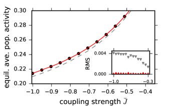
Figure 1: Convergence of the average population activity to the steady-state MFT predictions. The red line indicates the predictions of complete MFT up to fifth order correction. The dashed gray line is the predictions of mean-field eqn. 12, assuming only Gaussian fluctuations. The black dots represent network simulations averaged over 20 independent trails (error bars are smaller than symbol size). The inset is the Root Mean Square of error (RMS) between simulations and the complete theory (upward red triangles) and the Gaussian approximate theory (downward gray triangles). The simulations were performed using a Gillespie algorithm for $T=5\times 10^{5}$ steps with the gain function given by eqn. 16 . The averaged activity was estimated in the last $5\times 10^{3}$ steps across all trials. Parameters: $N=1000$, $\gamma=0.5$, $\alpha=5$, $K=10$ and $\mu_{0}=0.1$.

In order to demonstrate the applicability of our approach, we consider two scenarios that are relevant to the theoretical analysis of neural systems. The first scenario is that units receive a constant external input $\mu_{0}>0$. When $\bar{J}<0$ and $\gamma=0.5$ this system exhibits a nonequilibrium and chaotic state for which the external input is canceled by internal recurrent dynamics van Vreeswijk and Sompolinsky (1998). We choose a widely-used gain function in neural networks theory which it is given by

$$f(x):=\frac{1+\operatorname{Erf}(\alpha x)}{2}.$$ (16)

The parameter $\alpha$ describes the intrinsic noise intensity of the individual units and therefore must be positive. When $\alpha\rightarrow\infty$, this transfer function approximates to the well-studied Heaviside step function van Vreeswijk and Sompolinsky (1998); Dahmen et al. (2016). Using the transfer function given by eqn. 16 (with $\alpha=5$) and a directed fixed-in-degree Erdős-Rényi network (with $K=10$), we compute the complete steady-state mean-field limit using eqn. 13 by including up to the fifth order corrections (Fig.1, red line). We compare the complete MFT (Fig.1, red line) with the mean-field prediction that assumes only Gaussian statistics (i.e., $K\rightarrow\infty$) in eqn. 12 (Fig.1, dashed gray line). The difference between the predictions becomes apparent as $|\bar{J}|$ increases. Numerical simulations of a finite-size network ($N=1000$) are used to estimate the steady-state population activity by averaging 20 independent trials (Fig.1, black dots). The equilibrium population average activity of simulated networks (Fig.1, black dots) exhibits excellent agreement with both the complete (Fig.1, red line) and the Gaussian approximation (Fig.1, dashed gray line) of the mean-field limit in the case of weak coupling. However, in cases where the coupling is strong, the average population equilibrium activity deviates from the Gaussian approximation (Fig.1, dashed gray line) and, instead, follows the predictions of the complete mean-field limit (Fig.1, red line). Therefore, the Gaussian approximation that is given in eqn. 12 is only reasonable for weak coupling and relatively large value of $K$. The error between steady-state population activity from the simulations (Fig.1, black dots) and the Gaussian approximation (Fig.1, dashed gray line) increases as $|\bar{J}|$ becomes larger (Fig.1, downward gray triangles in the inset), in contrast to the complete MFT stays constant (Fig.1, upward red triangles in the inset).

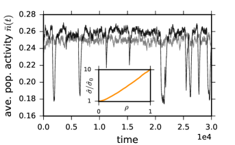
Figure 2: Emergence of stochastic MFT. The black line shows the temporal evolution of a simulated network; this network does not have a deterministic MFT since the condition in eqn. 10 is not satisfied. The out-degree of a single unit in the network was set to be $N$ (i.e., $\rho=1$ in eqn. 17). For comparison, the gray line shows the average population activity of a similar network for which $\rho=K/N$. The inset indicates the normalized empirical standard deviation of population activity temporal dynamics ($\hat{\sigma}/\hat{\sigma}_{0}$) as a function of $\rho$ (averaged over 20 independent trials with an expected number of 650 updates per unit). Simulations for the inset were performed using the stochastic update scheme described in van Vreeswijk and Sompolinsky (1998). Parameters: $N=5000$, $\bar{J}=-0.7$ and all other parameters are as in Fig.1.

In the second scenario, we show that an inherently stochastic mean-field limit with nontrivial fluctuations can emerge in a network with statistically inhomogeneous out-degrees. The condition in eqn. 10 guarantees the convergence of the average population activity to the prediction of MFT. Indeed eqn. 10 indicates that, as $N\rightarrow\infty$, the average column sum of the connectivity matrix $\mathbf{J}$ should be $K$. It is straightforward to construct networks that do not obey this rule; such networks lose their pointwise convergence to a deterministic MFT in eqn. 3. An extreme example of a network of this kind is a network that has a single unit, $n_{j_{*}}$, that connects into $\rho N$ units in the circuits, where $0<\rho\leq 1$ is the fraction of units in the network that are post-synaptic for $n_{j_{*}}$. Numerical simulations of such a network ($N=5000$ and $\rho=1$) show large-amplitude population activity fluctuations (Fig.2, black line), in contrast to the smaller fluctuations of a homogeneous network (Fig.2, gray line). Our approach allows the construction of stochastic correction terms to the mean-field limit by isolating the unit $n_{j_{*}}$ from the network and then taking the limit $N\rightarrow\infty$. Therefore, a first-order correction to the function $F$ of eqn. 7 can be derived as

$$F_{s}(m(t))\approx F(m(t))+\rho\bar{J}K^{-\gamma}f^{\prime}(\mu_{1}(t))n_{j_{*}}(t).$$ (17)

$F_{s}$ is a stochastic function since $n_{j_{*}}$ is a binomial random variable for which the probability of being at state one is $m(t)$; the mean-field equation is thus transformed into an ordinary stochastic differential equation. The correction term in eqn. 17 indicates that the observed large fluctuations (Fig.2, green line) are indeed a finite $K$ phenomenon. Therefore, in large networks that have a finite number of connections between units (e.g. finite $K$ networks), it suffices that only one unit breaks the condition (i.e., $\rho>0$) and, as a result, the deterministic MFT collapses (Fig.2, inset). The emergence of large-amplitude population events in Fig.2 has been observed previously as the indication of the “synfire chain” in cortical networks simulations Aviel et al. (2003). It is noteworthy that there is compelling evidence that a few neurons can form an extensive number of post-synaptic connections in cortical microcircuits Lee et al. (2016). In eqn. 17, we observe that a unit with a high out-degree can influence the macroscopic dynamics of the system. Therefore, recent experimental results that indicate the diverse couplings between single-cell activity and population averages in cortical networks Okun et al. (2015) can be the result of inhomogeneity of out-degrees.

In this letter, we studied a simplified model that captures the essential nonequilibrium aspects of cortical asynchronous state van Vreeswijk and Sompolinsky (1998), and it allowed us to demonstrate the calculation of a complete statistics of fluctuations in fixed indegree networks. Our results show that the MFT for binary units can be fundamentally constructed from the LLNs and the emergence of intrinsic fluctuations does not require the application of the central limit theorem. It is noteworthy that considering other heterogeneities in the system requires extra averaging operations and performing self-consistent calculations of temporal and spatial fluctuations. For instance, in a network in which unit $i$ has $K_{i}$ incoming connections, it can be shown that the power of $m$ in the eqn. 9 must be replaced by moments of the rate distribution, $\operatorname{E}\big{(}m^{r}\big{)}$, which can be self-consistently determined.

The semimartingale decomposition captures the finite-size effect (eqn. 15) in the orthogonal direction to the average correlations between units. These correlations have been investigated previously Renart et al. (2010). Here, the finite-size scaling of fluctuations can be derived directly form rate matrix $Q$. In a recent study by Dahmen et al. Dahmen et al. (2016) the MFT of binary units is extended by a cumulant expansion that allows the systematic calculation of finite-size corrections to cumulants of arbitrary order. In contrast, in our analysis all remaining correlations are implicitly encapsulated in the martingale part. Importantly, the application of martingale theory and the expansion of the averaging operator allows a tractable alternative to the perturbative expansion of the system’s state-space evolution to formulate an exact theory for network collective dynamics.

Our approach in this letter goes beyond the classical asymptotic analysis of random connectivities, which requires statistical conditions for connectivity matrices, $\mathbf{J}$, to ensure pointwise convergence to a deterministic MFT, irrespective of any fine or major motifs in the connectivity matrix, and suggests a universality class of MFT for all fixed-in-degree and iid networks. Furthermore, we demonstrated a computationally interesting phenomenon for emergence of a stochastic MFT by breaking the first condition (eqn. 10). Our framework can be readily exploited to determine the mean-field equilibrium of symmetrically disordered systems, in the presence of microstructures in their interactions such as spin glasses and associative neural networks Agliari et al. (2012); *sollich_extensive_2014, similarly. Once the connectivity matrix is given, it is straightforward to determine if the system’s mean population activity converges to the MFT in an annealed dynamics with independent initial conditions. In the quenched dynamics, the analysis of metastability requires a further investigation of the invariance measures of the state-space. Taken all together, we believe this approach paves the way for investigating the MFT of various networks collective phenomena.

Acknowledgment. This work was supported by the Federal Ministry of Education and Research (BMBF) Germany under grant No. FKZ01GQ1001B and Deutsche Forschungsgemeinschaft (DFG) grant No. FA1316/2-1.

References

- Mézard et al. (1986) M. Mézard, G. Parisi, and M. Virasoro, Spin Glass Theory and Beyond: An Introduction to the Replica Method and Its Applications, World Scientific Lecture Notes in Physics, Vol. 9 (World Scientific, 1986).
- Ising (1925) E. Ising, Zeitschrift für Physik 31, 253 (1925).
- Hohenberg and Halperin (1977) P. C. Hohenberg and B. I. Halperin, Reviews of Modern Physics 49, 435 (1977).
- Hamley (2013) I. W. Hamley, Introduction to Soft Matter: Synthetic and Biological Self-Assembling Materials (John Wiley & Sons, 2013).
- van Vreeswijk and Sompolinsky (1998) C. van Vreeswijk and H. Sompolinsky, Neural Comput 10, 1321 (1998).
- Glauber (1963) R. J. Glauber, Journal of Mathematical Physics 4, 294 (1963).
- Ginzburg and Sompolinsky (1994) I. Ginzburg and H. Sompolinsky, Physical Review E 50, 3171 (1994).
- Buice et al. (2010) M. A. Buice, J. D. Cowan, and C. C. Chow, Neural computation 22, 377 (2010).
- Renart et al. (2010) A. Renart, J. d. l. Rocha, P. Bartho, L. Hollender, N. Parga, A. Reyes, and K. D. Harris, Science 327, 587 (2010).
- Mézard and Sakellariou (2011) M. Mézard and J. Sakellariou, Journal of Statistical Mechanics: Theory and Experiment 2011, L07001 (2011).
- Stroock (2008) D. W. Stroock, An Introduction to Markov Processes, 2005th ed. (Springer, Berlin; New York, 2008).
- (12) .
- Gillespie (1976) D. T. Gillespie, Journal of Computational Physics 22, 403 (1976).
- Doob (1942) J. L. Doob, Transactions of the American Mathematical Society 52, 37 (1942).
- Dahmen et al. (2016) D. Dahmen, H. Bos, and M. Helias, Physical Review X 6, 031024 (2016).
- Stuard and Ord (1994) A. Stuard and J. K. Ord, Kendall’s Advanced Theory of Statistics. Vol. 1. Distribution Theory (Halsted Press, New York, NY, 1994).
- Brunel and Hakim (1999) N. Brunel and V. Hakim, Neural Computation 11, 1621 (1999).
- Mattia and Giudice (2002) M. Mattia and P. D. Giudice, in Artificial Neural Networks — ICANN 2002, Lecture Notes in Computer Science No. 2415, edited by J. R. Dorronsoro (Springer Berlin Heidelberg, 2002) pp. 111–116.
- Grytskyy et al. (2013) D. Grytskyy, T. Tetzlaff, M. Diesmann, and M. Helias, Frontiers in Computational Neuroscience 7 (2013), 10.3389/fncom.2013.00131.
- Aviel et al. (2003) Y. Aviel, C. Mehring, M. Abeles, and D. Horn, Neural computation 15, 1321 (2003).
- Lee et al. (2016) W.-C. A. Lee, V. Bonin, M. Reed, B. J. Graham, G. Hood, K. Glattfelder, and R. C. Reid, Nature 532, 370 (2016).
- Okun et al. (2015) M. Okun, N. A. Steinmetz, L. Cossell, M. F. Iacaruso, H. Ko, P. Barthó, T. Moore, S. B. Hofer, T. D. Mrsic-Flogel, M. Carandini, and K. D. Harris, Nature 521, 511 (2015).
- Agliari et al. (2012) E. Agliari, A. Barra, A. Galluzzi, F. Guerra, and F. Moauro, Physical Review Letters 109 (2012), 10.1103/PhysRevLett.109.268101.
- Sollich et al. (2014) P. Sollich, D. Tantari, A. Annibale, and A. Barra, Physical Review Letters 113 (2014), 10.1103/PhysRevLett.113.238106.