Local and non-local energy spectra of superfluid ³He turbulence

Abstract

Below the phase transition temperature $T_{\text{c}}\simeq 10^{-3}\,$K ³He-B has a mixture of normal and superfluid components. Turbulence in this material is carried predominantly by the superfluid component. We explore the statistical properties of this quantum turbulence, stressing the differences from the better known classical counterpart. To this aim we study the time-honored Hall-Vinen-Bekarevich-Khalatnikov coarse-grained equations of superfluid turbulence. We combine pseudo-spectral direct numerical simulations with analytic considerations based on an integral closure for the energy flux. We avoid the assumption of locality of the energy transfer which was used previously in both analytic and numerical studies of the superfluid ³He-B turbulence. For $T<0.37\,T_{\text{c}}$, with relatively weak mutual friction, we confirm the previously found “subcritical” energy spectrum $E(k)$, given by a superposition of two power laws that can be approximated as $E(k)\propto k^{-x}$ with an apparent scaling exponent $\frac{5}{3}<x(k)<3$. For $T>0.37\,T_{\text{c}}$ and with strong mutual friction, we observed numerically and confirmed analytically the scale-invariant spectrum $E(k)\propto k^{-x}$ with a ($k$-independent) exponent $x>3$ that gradually increases with the temperature and reaches a value $x\sim 9$ for $T\approx 0.72\,T_{\text{c}}$. In the near-critical regimes we discover a strong enhancement of intermittency which exceeds by an order of magnitude the corresponding level in classical hydrodynamic turbulence.

Introduction

Helium below the phase transition temperatures $T_{\lambda}\simeq 2.1\,$K in ⁴He and $T_{\text{c}}\simeq 10^{-3}\,$K in ³He can be described as consisting of two coupled, interpenetrating fluids. One fluid is inviscid with quantized vorticity, and the second is viscous with a continuous vorticity. Consequently, superfluid turbulence is even more complex than turbulence in classical fluids. Moreover, the present knowledge of many aspects of superfluid turbulence is still not fully developed despite the many decades since the discovery of superfluidity, see, e.g. Refs. Rev1 ; Rev2 ; Rev3 ; Rev4 . The subject offers many opportunities for new approaches and new discoveries.

From the experimental point of view the study of the statistical properties of superfluid turbulence is still difficult, even with the use of state-of-the-art technologies. The very low values of $T_{\lambda}$ and $T_{\text{c}}$ limit severely any visual access, and in addition pose problems for adequate sensors Rev1 ; Rev2 ; Rev3 ; Rev4 . Nevertheless new experiments are emerging, requiring parallel theoretical efforts. Theoretical progress requires developing direct numerical simulations (DNS) which presently are the only way to reach a complete description of the evolution of the normal and superfluid velocity components. Such data offer access to the statistical properties of superfluid turbulence. In the present paper we study the physics of superfluid ³He turbulence, using the fact that it is simpler problem than turbulence in ⁴He, due to very high viscosity of the normal component, which may be considered laminar.

The energy spectra $E(k)$ in space-homogeneous, steady and isotropic turbulence in superfluid ³He were studied analytically within the algebraic approximation for the energy flux in LABEL:LNV (see also Eq. (2b) below). Numerically the issue was studied using the Sabra-shell model in LABEL:He3a. The two papers  LNR ; He3a considered the large-scale velocity fluctuations with $k<\pi/\ell$, where $\ell$ is the mean distance between quantized vortex lines. It was shown that the mutual friction between normal and superfluid components suppresses $E(k)$ with respect of the Kolmogorov-1941 (K41) prediction Fri :

$$E^{{}^{\text{K41}}}(k)=C_{\scriptscriptstyle\rm{K}}\varepsilon_{0}^{2/3}k^{-5/3}\ .$$ (1)

Here $\varepsilon_{0}$ is the energy flux over scales, equal in this case to the rate of energy input into the system at $k=k_{0}$: $\varepsilon_{0}=\varepsilon(k_{0})$; $C_{\scriptscriptstyle\rm{K}}\sim 1$ is the dimensionless Kolmogorov constant.

The isotropic, steady-state energy balance equation in a one-fluid approach to ³He turbulence was analyzed by Lvov, Nazarenko and Volovik (LNV) in LABEL:LNV:

$$\frac{d\,\varepsilon(k)}{dk}+\Omega\,E(k)=0\,,\quad\Omega=\alpha(T)\,\Omega_{\scriptscriptstyle\rm{T}}\ .$$ (2a)

Here $$\alpha(T) \Omega_{\scriptscriptstyle\rm{T}} \varepsilon(k)$$ is the temperature dependent dimensionless mutual friction parameter and is the root mean square (rms) turbulent vorticity. The wavenumber-dependent energy flux over scales, , was approximated in LABEL:LNV using K41-type dimensional reasoning, similar to Eq. (1):

$$\varepsilon(k)=\big{[}E(k)\big{/}C_{\scriptscriptstyle\rm{K}}\big{]}^{3/2}\,k^{5/2}=\frac{8}{3}\big{[}E(k)\big{]}^{3/2}\,k^{5/2}\,,$$ (2b)

as suggested by Kovasznay Kov .

The ordinary differential Eq. (2) has an analytical solution LNV :

$$E(k) = E^{{}^{\text{K41}}}(k)\Big{[}1-\Omega^{\dagger}+\Omega^{\dagger}\Big{(}\frac{k_{0}}{k}\Big{)}^{2/3}\Big{]}^{2},\ \mbox{where}~{}~{}~{}~{}~{}~{}~{}~{}$$ (3a)

$$\Omega^{\dagger} = \frac{\Omega}{\Omega_{\text{cr}}}\,,\quad\Omega_{\text{cr}}=\frac{5}{4}\,\sqrt{k_{0}^{3}\,E_{0}}\,,\quad E_{0}\equiv E(k_{0})\ .$$ (3b)

For $$\Omega^{\dagger}<1$$ Eq. (3a) introduces a new crossover length-scale

$$k_{\times}=k_{0}\big{[}\Omega^{\dagger}\big{/}(1-\Omega^{\dagger})\big{]}^{3/2}\,,$$ (3c)

that breaks the scaling invariance, predicting for $$\Omega<\Omega_{\text{cr}} k\ll k_{\times}$$ a superposition of two scaling laws:
– For small , the LNV spectrum (3a) takes a “critical” form

$$E_{\text{cr}}(k)=E_{0}\big{(}k_{0}/k\big{)}^{3}\ .$$ (3d)

– For large enough $$k\gg k_{\times} \varepsilon_{\infty}<\varepsilon_{0} \varepsilon_{0}-\varepsilon_{\infty} k\sim k_{\times} E(k)\propto k^{-x} \frac{5}{3}<x(k)<3$$, the K41 spectrum (1) is recovered, but with the energy flux . The difference is dissipated by the mutual friction. For , the energy spectrum can be roughly approximated as with an apparent scaling exponent .

The crossover wavenumber $k_{\times}$ increases with $\alpha(T)$ and for some critical value of $\alpha_{\text{cr}}\sim 1$ it diverges. Then the critical LNV-spectrum (3d) occupies the entire available interval $k_{0}<k<\pi/\ell$.

For $\alpha(T)>\alpha_{\text{cr}}$, the spectrum (3a) becomes “supercritical” and terminates at some final $k_{*}$ that depends on $\alpha(T)$:

$$E_{\text{s}}(k)\propto k^{-3}\big{[}k_{*}^{2/3}-k^{2/3}\big{]}^{2}\ .$$ (3e)

All types of the LNV spectra (subcritical, critical and supercritical) where observed in Sabra-shell model simulations (see Refs. He3a and lb for a general review on shell models). However, the analytical LNV model LNV is based on an uncontrolled algebraic approximation for the energy flux (2b); the shell-model of turbulence, used in LABEL:He3a, is also an uncontrolled simplification of the basic equations of motion for the superfluid velocity field. Therefore, the problem of turbulent energy spectra in superfluid ³He requires further investigation.

In this paper we report results of a first (to the best of our knowledge) DNS study of the statistical properties of a space-homogeneous, steady and isotropic turbulence in superfluid ³He. We provide results on the turbulent energy spectra, the velocity and vorticity structure functions at different temperatures $0<T<0.7T_{\text{cr}}$, the energy balance and intermittency effects. To these aims we use the gradually-damped version of the Hall-Vinen HV -Bekarevich-KhalatnikovBK (HVBK) coarse-grained two-fluid model Eq. (4) as suggested in LABEL:PRB. We expect this model to describe properly the turbulent velocity fluctuations in superfluid ⁴He and ³He as long as the their scales exceed the mean intervortex distance $\ell$.

The paper is organized as follows:
 
• Section I is devoted to an analytical description of the statistical properties of the steady, homogeneous, isotropic, incompressible turbulence of superfluid ³He. This should serve as a basis for further studies of superfluid turbulence in more complicated or/and realistic cases: anisotropic turbulence, transient regimes, two-fluid turbulence of counterflowing, thermally driven, superfluid ⁴He turbulence, etc.

In Sec. I.1 we present the gradually damped HVBK Eqs. (4);

In Sec. I.2 we introduce the required statistical objects.

In Sec. I.3 we adapt the integral closureLNR to obtain the energy spectrum when the energy transfer over scales is not local.

In Sec. I.4 we analyze the relations between the structure functions of the velocity and vorticity fields with the sub- and super-critical energy spectra $E(k)$. These are required for the analysis of the DNS data.

• Section II presents the DNS results for the statistics of superfluid turbulence in ³He, together with a comparison with the theoretical expectations.

In Sec. II.1 we shortly describe the details of the numerical procedure;

In Sec. II.2 we present the DNS results for the energy spectra obtained for different values of mutual friction frequency $\Omega$ in the subcritical, critical and supercritical regimes. We demonstrate their quantitative agreement with the corresponding theoretical predictions, given by Eqs. (3a), (3d) and (16);

In Sec. II.3 we report a significant enhancement of intermittency in near-critical regimes of superfluid ³He turbulence, revealed by analysing the second- and fourth-order structure functions of the velocity and vorticity differences;

In Sec. II.4 we analyze the energy balance in the entire region of $k$, shedding light on the origin of the subcritical, critical and supercritical regimes of the energy spectra;

In Sec. II.5 we present and analyze the DNS results for the energy and enstropy time evolution, showing how the large and small scale turbulent fluctuations are correlated (or uncorrelated) in different regimes;

Section II.6 clarifies the relation between the mutual friction frequency $\Omega$ and the temperature $T$ in possible experiments.

• Section III summarizes our findings. For the convenience of the reader we present here the main results:

The numerical subcritical energy spectra for different $T<0.37\,T_{\text{cr}}$ (see Tab. 1 and Fig. 1a), are in good agreement with the LNV prediction (3a) with a single fitting parameter $b\approx 0.5$ that replaces the factor $\frac{5}{4}$ in Eq. (3b).

At $T\approx 0.37\,T_{\text{cr}}$ (corresponding to $\Omega=0.9$ in our case) we observed a critical energy spectrum $E_{\text{cr}}\propto 1/k^{3}$.

The numerically observed supercritical energy spectra at $T>0.37\,T_{\text{cr}}$ exhibit a scale-invariant behavior $E(k)\propto k^{-x}$, Eq. (16a) with the scaling exponent $x>3$ that gradually increases with the temperature and reaches the value $x\sim 9$ for $T\approx 0.72\,T_{\text{cr}}$.

Relaxing the assumption of locality by using integral closure for the energy flux (11), we confirmed analytically the scale-invariant spectrum $E(k)\propto k^{-x}$, Eq. (16a) with the variable scaling exponent $x$ that depends on the temperature in a qualitative agreement with the DNS observation.

In the near-critical regimes we observed significant increase in turbulent fluctuations of superfluid velocity and vorticity at small scales, typical for intermittency.

I Analytic Discussion of the Statistics of $\bm{}3$He turbulence

I.1 Gradually damped HVBK-equations for superfluid ³He-B turbulence

Large scale turbulence in superfluid ³He can be described by the Landau-Tisza two-fluid model in which the interpenetrating normal and superfluid components have densities $\rho_{\text{n}}$, $\rho_{\text{s}}$ and velocity fields ${\bm{u}}_{\text{n}}({\bm{r}},t)$, ${\bm{u}}_{\text{s}}({\bm{r}},t)$, respectively. The gradually damped version of the coarse-grained HVBK equations PRB for incompressible motions of superfluids with constant densities has the form of two Navier-Stokes equations supplemented by mutual friction:

$$\hskip-36.98866pt\frac{\partial\,{\bm{u}}_{\text{s}}}{\partial t}+({\bm{u}}_{\text{s}}\cdot{\bm{\nabla}}){\bm{u}}_{\text{s}}-\frac{1}{\rho_{\text{s}}}{\bm{\nabla}}p_{\text{s}}=\nu_{\text{s}}\,\Delta{\bm{u}}_{\text{s}}+{\bm{f}}_{\text{ns}}\,,$$

$$\hskip-36.98866pt\frac{\partial\,{\bm{u}}_{\text{n}}}{\partial t}+({\bm{u}}_{\text{n}}\cdot{\bm{\nabla}}){\bm{u}}_{\text{n}}-\frac{1}{\rho_{\text{n}}}{\bm{\nabla}}p_{\text{n}}=\nu_{\text{n}}\,\Delta{\bm{u}}_{\text{n}}{\bm{-}}\frac{\rho_{\text{s}}}{\rho_{\text{n}}}{\bm{f}}_{\text{ns}}\,,$$

$$\hskip-36.98866ptp_{\text{n}}=\frac{\rho_{\text{n}}}{\rho}[p+\frac{\rho_{\text{s}}}{2}|{\bm{u}}_{\text{s}}-{\bm{u}}_{\text{n}}|^{2}]\,,p_{\text{s}}=\frac{\rho_{\text{s}}}{\rho}[p-\frac{\rho_{\text{n}}}{2}|{\bm{u}}_{\text{s}}-{\bm{u}}_{\text{n}}|^{2}]\,,$$

$${\bm{f}}_{\text{ns}} \simeq \alpha(T)\,\Omega_{\scriptscriptstyle\rm{T}}\,({\bm{u}}_{\text{n}}-{\bm{u}}_{\text{s}})\,.$$ (4c)

Here $p_{\text{n}}$, $p_{\text{s}}$ are the pressures of the normal and the superfluid components. $\rho\equiv\rho_{\text{s}}+\rho_{\text{n}}$ is the total density, $\nu_{\text{n}}$ is the kinematic viscosity of normal fluid component. The dissipative term with the Vinen’s effective superfluid viscosity $\nu_{\text{s}}$ was added in LABEL:He4 to account for the energy dissipation at the intervortex scale $\ell$ due to vortex reconnections and similar effects. A qualitative estimate of the effective viscosity $\nu_{\text{s}}\simeq\alpha\kappa\rho_{\text{s}}/\rho$ follows from a model of a random vortex tangle moving in a quiescent normal component He4 .

The approximate Eq. (4c) for the mutual friction force ${\bm{f}}_{\text{ns}}$ was suggested in LABEL:LNV. It involves the temperature dependent dimensionless mutual friction parameters $\alpha(T)$ and rms superfluid turbulent vorticity $\Omega_{\scriptscriptstyle\rm{T}}$. In isotropic turbulence

$$\Omega_{\scriptscriptstyle\rm{T}}^{2}\equiv\left\langle|{\bm{\omega}}|^{2}\right\rangle\approx 2\int k^{2}E_{\text{s}}(k)dk\,,$$ (5)

where $E_{\text{s}}(k)$ is the one-dimensional (1D) energy spectrum, normalized such that the total energy density per unit mass ${\mathcal{E}}_{\text{s}}=\int E_{\text{s}}(k)\,dk$.

Note that in Eq. (4) we did not account for the reactive part of the mutual friction Sonin , proportional to another temperature dependent parameter $\alpha^{\prime}$. As was shown in LABEL:Finne, this force leads to a renormalization of the nonlinear terms in Eq. (4) by a factor $(1-\alpha^{\prime})$. Dividing Eq. (4) by this factor, we see that (besides the renormalization of time) we get also the renormalization of $\alpha\Rightarrow\widetilde{\alpha}=\alpha/(1-\alpha^{\prime})$ in Eq. (4c), which now reads:

$${\bm{f}}_{\text{ns}}\simeq\Omega\,({\bm{u}}_{\text{n}}-{\bm{u}}_{\text{s}})\,,\ \Omega=\widetilde{\alpha}(T)\,\Omega_{\scriptscriptstyle\rm{T}}\,,\ \widetilde{\alpha}=\alpha/(1-\alpha^{\prime})\ .$$ (6)

Ideally, the turbulent vorticity $\Omega_{\scriptscriptstyle\rm{T}}$ should be calculated self-consistently, at each time step. However we use a simplified version, by first solving Eqs. (4) with some value of $\Omega$, then calculating $\Omega_{\scriptscriptstyle\rm{T}}$ by Eq. (5) with the observed $E_{\text{s}}(k)$ and finally finding $\alpha^{{}^{\text{DNS}}}=\Omega/\Omega_{\scriptscriptstyle\rm{T}}$. After that we identify the temperature to which the particular simulation corresponds by comparing with known experimental values $\alpha(T)=\alpha^{{}^{\text{DNS}}}$. We have verified that in the present range of parameters, simulations with a constant value of $\Omega$ and self-consistent simulations give similar results.

I.2 Statistical description of space-homogeneous, isotropic turbulence of superfluid ³He

I.2.1 Definition of 1-D energy spectra and cross-correlations

Traditionally one describes the energy distribution over scales in a space-homogeneous, isotropic case using the one-dimensional (1D) energy spectrum $E(k)$, defined by Eq. (9). To clarify this definition we need to recall some well known relationships.

Fourier transforms are defined with the following normalization:

$${\bm{u}}_{\text{n,s}}({\bm{r}},t) \equiv \int\frac{d{\bm{k}}}{(2\pi)^{3}}\,\widetilde{{\bm{u}}}_{\text{n,s}}({\bm{k}},t)\exp(i{\bm{k}}\cdot{\bm{r}})\,,$$ (7a)

$$\widetilde{{\bm{u}}}_{\text{n,s}}({\bm{k}},t) = \int d{\bm{r}}~{}{\bm{u}}_{\text{n,s}}({\bm{r}},t)\exp(-i{\bm{k}}\cdot{\bm{r}})\ .~{}~{}~{}~{}~{}~{}~{}$$ (7b)

Next we define the simultaneous correlations and cross-correlations in ${\bm{k}}$-representation, [proportional to $\delta({\bm{k}}+{\bm{q}})$ and $\delta({\bm{k}}+{\bm{q}}+{\bm{p}})$ due to the space homogeneity]:

$$\left\langle\widetilde{{\bm{u}}}_{\text{n}}({\bm{k}},t)\cdot\widetilde{{\bm{u}}}_{\text{n}}({\bm{q}},t)\right\rangle=(2\pi)^{3}F_{\text{nn}}({\bm{k}})\,\delta({\bm{k}}+{\bm{q}})\,,~{}~{}~{}$$

$$\left\langle\widetilde{{\bm{u}}}_{\text{s}}({\bm{k}},t)\cdot\widetilde{{\bm{u}}}_{\text{s}}({\bm{q}},t)\right\rangle=(2\pi)^{3}F_{\text{ss}}({\bm{k}})\,\delta({\bm{k}}+{\bm{q}})\,,$$

$$\left\langle\widetilde{{\bm{u}}}_{\text{n}}({\bm{k}},t)\cdot\widetilde{{\bm{u}}}_{\text{s}}({\bm{q}},t)\right\rangle=(2\pi)^{3}F_{\text{ns}}({\bm{k}})\,\delta({\bm{k}}+{\bm{q}})\,,$$

$$\left\langle\widetilde{u}^{\,\xi}_{\text{s}}({\bm{k}},t)\,\widetilde{u}^{\,\beta}_{\text{s}}({\bm{q}},t)\,\widetilde{u}^{\,\gamma}_{\text{s}}({\bm{p}},t)\right\rangle$$

$$= (2\pi)^{3}F^{\xi\beta\gamma}_{\text{sss}}({\bm{k}},{\bm{q}},{\bm{p}})\,\delta({\bm{k}}+{\bm{q}}+{\bm{p}})\ .$$ (8d)

In the isotropic case the correlations $F_{\text{nn}}$, $F_{\text{ss}}$ and $F_{\text{ns}}$ become independent of the direction of ${\bm{k}}$, being functions of the wavenumber $k$ only. This allows us to introduce the one-dimensional energy spectra $E_{\text{s}}$, $E_{\text{n}}$ and the cross-correlation $E_{\text{ns}}$ as follows:

$$E_{\text{n}}(k) = \frac{k^{2}}{2\pi^{2}}F_{\text{nn}}(k)\,,\quad E_{\text{s}}(k)=\frac{k^{2}}{2\pi^{2}}F_{\text{ss}}(k)\,,$$

$$E_{\text{ns}}(k) \equiv \frac{k^{2}}{2\pi^{2}}F_{\text{ns}}(k)\ .$$ (9)

I.2.2 Energy balance equation

To derive the energy balance equation for $E_{\text{s}}(k,t)$ we first need to Fourier transform Eq. (4) to get the equation for $\widetilde{{\bm{u}}}_{\text{s}}({\bm{k}},t)$. Next, using Eq. (8) and Eq. (9), we arrive to the required balance equation:

$$\frac{\partial E_{\text{s}}(k)}{\partial t}+\mbox{Tr}(k)+\mbox{D}_{\nu}(k)+\mbox{D}_{\alpha}(k)=0\,,$$ (10a)

$$\mbox{D}_{\nu}=2\,\nu_{\text{s}}k^{2}E_{\text{s}}(k)\,,\ \mbox{D}_{\alpha}=2\,\Omega\big{[}E_{\text{s}}(k)-E_{\text{ns}}(k)\big{]}\ .~{}~{}~{}~{}$$ (10b)

Here D_ν describes the energy dissipation, caused by the effective viscosity. The term D_α is responsible for the energy dissipation by the mutual friction with the characteristic frequency $$\Omega$$ given by Eqs. (4c) and (5).

The energy transfer term Tr$(k)$ in Eq. (10a) originates from the nonlinear terms in the HVBK Eqs. (4) and has the same form as in classical turbulence (see, e.g. Refs. LP-95 ; LP-2 ):

$$\mbox{Tr}({\bm{k}}) = 2\,\mbox{Re}\Big{\{}\int V^{\xi\beta\gamma}({\bm{k}},{\bm{q}},{\bm{p}})\,F^{\xi\beta\gamma}({\bm{k}},{\bm{q}},{\bm{p}})$$ (10c)

$$\times\delta({\bm{k}}+{\bm{q}}+{\bm{p}})\frac{d^{3}q\,d^{3}p}{(2\pi)^{6}}\,\Big{\}}\,,$$

$$V^{\xi\beta\gamma}({\bm{k}},{\bm{q}},{\bm{p}}) = i\Big{(}\delta_{\xi\xi^{\prime}}-\frac{k^{\xi}k^{\xi^{\prime}}}{k^{2}}\Big{)}$$ (10d)

$$\times\Big{(}k^{\beta}\delta_{\xi^{\prime}\gamma}+k^{\gamma}\delta_{\xi^{\prime}\beta}\Big{)}\ .$$

Importantly, Tr$(k)$ preserves the total turbulent kinetic energy: $\displaystyle\int_{0}^{k}\mbox{Tr}(k^{\prime})dk^{\prime}=0$ and therefore can be written in the divergent form:

$$\mbox{Tr}(k)=\frac{\partial\,\varepsilon(k)}{dk}\,,$$ (10e)

where $\varepsilon(k)$ is the energy flux over scales.

I.3 Supercritical energy spectra

I.3.1 LNR integral closure

To relax the assumption of the local energy transfer in deriving the supercritical superfluid energy spectrum, we use the integral closure, introduced by L’vov, Nazarenko and RudenkoLNR (LNR). The main approximation in this closure is the presentation of the third order velocity correlation function $F^{\xi\beta\gamma}_{\text{sss}}$ in Eq. (10c) as a product of the vertex $V$, Eq. (10d), two second order correlations $F_{\text{ss}}(k_{j})$, Eq. (8), and response (Green’s) functions. This closure is widely used in analytic theories of classical turbulence, for example in the Eddy-damped quasinormal Markovian closure (EDQNM) (see, e.g. books LABEL:Fri,DKS ). Keeping in mind the uncontrolled character of this approximation, LNR further simplified the resulting approximation for isotropic turbulence by replacing $d^{3}q\,d^{3}p\,\delta^{3}({\bm{k}}+{\bm{q}}+{\bm{p}})$ in Eq. (10c) with 3-dimensional vectors ${\bm{k}}$, ${\bm{q}}$, and ${\bm{p}}$   by  $q^{2}dq\,p^{2}dp\ \delta(k+q+p)/(k^{2}+q^{2}+p^{2})$ with one-dimensional vectors $k$, $q$, and $p$ varying in the interval $(-\infty,+\infty)$. The next simplification is the replacement of the interaction amplitude $V^{\xi\beta\gamma}({\bm{k}},{\bm{q}},{\bm{p}})$, Eq. (10d) by its scalar version $(ik)$. The resulting LNR closure can be written as follows:

$$\mbox{Tr}(k)=\frac{A_{1}\,k^{3}}{2\pi^{2}}\int_{-\infty}^{\infty}\frac{q^{2}dq\,p^{2}dp\,\delta(k+q+p)}{2\pi\,(k^{2}+q^{2}+p^{2})}$$ (11)

$$\hskip-14.22636pt\times\frac{k\,F_{\text{ss}}(|q|)F_{\text{ss}}(|p|)+q\,F_{\text{ss}}(|k|)F_{\text{ss}}(|p|)+p\,F_{\text{ss}}(|q|)F_{\text{ss}}(|k|)}{\Gamma(|k|)+\Gamma(|q|)+\Gamma(|p|)}.$$

Here $A_{1}$ is a dimensionless parameter of the order of unity and $\displaystyle\Gamma(k)$ is the typical relaxation frequencies on the scale $k$.

The LNR model (11) satisfies all the general closure requirements: it conserves energy, $\int\mbox{Tr}(k)\,dk=0$ for any $F_{k}$; Tr$(k)=0$ for the thermodynamic equilibrium spectrum $F_{k}=$const and for the cascade K41 spectrum $F(k)\propto|k|^{-11/3}$. Importantly, the integrand in Eq. (11) has the correct asymptotic behavior at the limits of small and large $q/k$, as required by the sweeping-free Belinicher-L’vov representation, see LABEL:BL. This means that the model (11) adequately reflects contributions of the extended interaction triads and thus can be used for the analysis of the supercritical spectra.

I.3.2 Supercritical spectra with non-local energy transfer

As was shown in LABEL:Kh15, the eddy life time in ³He turbulence is restricted by the mutual friction, which dominates the dissipation due to the effective viscosity $\nu_{s}k^{2}$ and the turbulent viscosity, caused by the eddy interactions. Therefore we can safely approximate $\Gamma(k)$ in Eq. (11) by $\Omega$. Omitting further the (uncontrolled) prefactors of the order of unity and using Eq. (9), we rewrite Tr$(k)$ in Eq. (10a) as follows

$$\mbox{Tr}(k) \simeq -\frac{A\,k}{\Omega}\int\limits_{-\infty}^{\infty}\frac{dq\,dp\,\delta(k+q+p)}{k^{2}+q^{2}+p^{2}}$$

$$\hskip-42.67912pt\times{\big{[}k^{3}\,E_{\text{s}}(|q|)E_{\text{s}}(|p|)+q^{3}E_{\text{s}}(|k|)E_{\text{s}}(|p|)+p^{3}\,E_{\text{s}}(|q|)E_{\text{s}}(|k|)\big{]}}\ .$$

Here $A$ is uncontrolled dimensionless parameter, presumably of the order of unity. Recall, that in ³He turbulence $E_{\text{n}}\ll E_{\text{s}}$ and $E_{\text{ns}}\ll E_{\text{s}}$. This allows us to simplify the mutual friction dissipation term D_α to the form D${}_{\alpha}(k)\approx 2\,\Omega E_{\text{s}}(k)$. Hereafter we consider only superfluid component and omit the superscript ”s“ in notations. We show below that in the supercritical regime the viscous dissipation term D${}_{\nu}(k)$ is vanishingly small with respect to the mutual friction term D${}_{\alpha}(k)$ and therefore can be neglected in the balance Eq. (10a). Thus, in the stationary case Eq. (10a) can be presented in a simple form:

$$\mbox{Tr}(k)+2\,\Omega\,E(k)=0\ .$$ (12b)

The integral (I.3.2) diverges in the regions $q\ll k$ or $p\ll k$. For these wavenumbers it can be approximated as:

$$\mbox{Tr}(k) \simeq -\frac{A\,k}{\Omega}\int\limits_{-\infty}^{\infty}E(|q|)\Psi(k,q)dq\,,$$ (13)

$$\Psi(k,q) = \frac{k^{3}\,E(|k+q|)-(k+q)^{3}\,E(|k|)}{k^{2}+q^{2}+(k+q)^{2}}\ .$$

One sees that for $q=0$ $\Psi(k,0)=0$ and the term which is linear in $q$ in the expansion does not contribute to the integral (13). Therefore the main contribution to this integral in the region $q\ll k$ originates from the second term of the expansion:

$$\Psi(k,q)\simeq\frac{q^{2}}{2}\frac{\partial^{2}\Psi}{\partial q^{2}}\Big{|}_{q=0}=\frac{q^{2}}{2}\Big{[}\frac{k}{2}E^{\prime\prime}(k)-E^{\prime}(k)\Big{]}\,.$$ (14)

Here ^′ indicates the derivative with respect to $k$. Now the energy balance Eqs. (12) can be simplified as follows:

$$A\,\Omega_{\scriptscriptstyle\rm{T}}^{2}k\Big{[}\frac{k}{2}E^{\prime\prime}(k)-E^{\prime}(k)\Big{]}=4\,\Omega^{2}\,E(k)\,,$$ (15)

where $\Omega_{\scriptscriptstyle\rm{T}}$ is given by Eq. (5). Equation (15) has the scale invariant solutions

$$E(k)\propto k^{-x}\,,$$ (16a)

with

$$A\,\Omega_{\scriptscriptstyle\rm{T}}^{2}\,x(x-1)=8\,\Omega^{2}\ .$$ (16b)

The whole approach is valid if the main contribution to the integral (5) comes from the region $$q\ll k_{\text{max}} x>3 x=3 \Omega x>3$$, i.e for supercritical cases with . With logarithmic accuracy we can also include the critical case with . This allows us to estimate the new critical value of for supercritical regimes (with ):

$$\widetilde{\Omega}_{\text{cr}}=\Omega_{\scriptscriptstyle\rm{T}}\sqrt{3A}/2\ .$$ (16c)

Now we can rewrite Eq. (16b) as:

$$x(x-1)=6\,(\Omega^{\ddagger})^{2}\,,\quad\Omega^{\ddagger}\equiv\Omega/\widetilde{\Omega}_{\text{cr}}\,,\quad x>3\ .$$ (16d)

We thus conclude that for the integral closure (I.3.2) that takes into account the long-distance energy transfer in $k$-space, the supercritical spectra do not terminate at some final value of $k$ [as with the algebraic closure (2b)], but behave like $E(k)\propto k^{-x}$ with a scaling exponent $x>3$ that increases with the supercriticality $\Omega^{\ddagger}$.

I.4 Relations between structure functions and energy spectra

Velocity structure function $S_{2}(r)$ vs $E(k)$.

Consider full 2${}^{\text{nd}}$-order velocity structure function

$$S_{2}(r)\equiv\left\langle|{\bm{v}}({\bm{r}}+{\bm{R}})-{\bm{v}}({\bm{R}})|^{2}\right\rangle\,,$$ (17a)

which is related to the 3D energy spectrum $F(k)$ as follows:

$$S_{2}(r) = \int\frac{d^{3}k}{(2\pi)^{3}}\,|1-\exp(i{\bm{k}}\cdot{\bm{r}})|^{2}F(k)$$

$$= 2\int\frac{d^{3}k}{(2\pi)^{3}}\big{[}1-\cos({\bm{k}}\cdot{\bm{r}})\big{]}F(k)\ .$$

In spherical coordinates:

$$S_{2}(r) = 2\int E(k)\Big{[}1-\frac{\sin(kr)}{kr}\Big{]}dk\ .$$ (18)

Let us analyze convergence of this integral for scale-invariant spectra $E(k)\propto k^{-x}$. In the ultraviolet (UV) region (for $k\,r\gg 1$) the oscillating term ($\propto\sin(k\,r)$) can be neglected and the integral (18) converges if $x>1$. In the infrared (IR) region (for small $k\,\ll 1$)

$$[1-\sin(k\,r)/(k\,r)]\simeq(k\,r)^{2}/6$$ (19)

and the integral (18) converges if $x<3$. We conclude that for the integral (18) the window of convergence (more often is referred to as the locality window) is:

$$1<x<3\,,\quad\mbox{Locality window for $S_{2}$ integral.}$$ (20a)

In this window, the leading contribution to the integral (18) comes from the region $$k\,r\sim 1$$ and

$$S_{2}(r)\propto r^{y}\,,\quad y=x-1\ .$$ (20b)

This is a well know relationship. For example, for the K41 spectrum with $x=5/3$ (which is inside the locality window (20a)) $y=2/3$ .

We conclude that subcritical spectra, (which in the finite-$k$ interval can be approximated as $E(k)\propto k^{-x}$ with $\frac{5}{3}\leq x\leq 3$) are local and we can use for the estimate of the $S_{2}$ the scaling relation (20b). We also see that when exponent $x$ approaches the critical value $x=3$, the $S_{2}$ scaling approaches the viscous limit with $y=2$. For $x=3$, $S_{2}(r)\propto r^{2}$ with logarithmic corrections, not detectable with our resolution.

In the supercritical region ($x>3$), the $S_{2}$-integral(18) formally IR-diverges and the integration region has to be restricted from below by some $k_{0}$, similarly to the integral (5). Together with Eq. (19), this gives the viscous behavior for any $x>3$:

$$S_{2}(r)\simeq(r\,\Omega_{\scriptscriptstyle\rm{T}})^{2}/6\ .$$ (21)

Table 1: Parameters used in the simulations by columns: (# 1) $\Omega$ determines the mutual friction by Eqs. (4c) and (5); (# 2) $\nu_{s}$: the effective viscosity of the superfluid component; (# 3) $u^{\text{s}}_{\rm rms}$: the rms velocity of the superfluid component; (# 4) $Re^{\text{s}}_{\lambda}=u^{\text{s}}_{\rm rms}\lambda/\nu_{s}$: the Taylor-microscale Reynolds number, where $\displaystyle\lambda=\frac{2\pi}{L}\sqrt{\frac{\langle u^{2}\rangle}{\langle\omega^{2}\rangle}}$ is the Taylor microscale; (# 5) $\varepsilon^{\text{s}}_{\nu}$: the mean energy dissipation rate for the superfluid component due to viscosity; (# 6) $\varepsilon^{\text{s}}_{\rm tot}$: total mean energy dissipation rate for the superfluid component; (#7) $\eta_{s}=\sqrt{2}\nu_{s}/u^{\text{s}}_{\rm rms}$; (# 8) $T^{\text{s}}_{0}=L/u^{\text{s}}_{\text{rms}}$: large-eddy-turnover time. The temperature dependence of $\widetilde{a}$ is taken from Ref.Bevan (see Fig. 7). In all simulations: the number of collocation points along each axis is $N=1024$; the size of the periodic box is $L=2\pi$; the kinematic viscosity of the normal component is $\nu_{n}=10$; the range of forced wavenumbers $k^{\varphi}=[0.5,1.5]$. The values for the critical value of $\Omega_{\text{cr}}\approx\Omega=0.9$ [row (#5)] are emphasized. Runs (#1-#4) correspond to the subcritical regime, (#6-#8) to the supercritical regime.

#	1	2	3	4	5	6	7	8	9	10	11	12	13	14	15
#	$\Omega$	$\nu_{s}$	$u^{s}_{\rm rms}$	$Re^{s}_{\lambda}$	$\varepsilon^{s}_{\nu}$	$\varepsilon^{s}_{\rm tot}$	$\eta_{s}$	$T_{0}^{s}$	$\Omega_{\text{cr}}$	$\widetilde{\Omega}_{\text{cr}}\approx$	$\Omega^{\dagger}=$	$\Omega^{\ddagger}=$	$\Omega_{\scriptscriptstyle\rm{T}}$	$1/\widetilde{\alpha}(T)$	$T/T_{\text{c}}$
	Eq. (6)	$\times 10^{4}$					$\times 10^{4}$		Eq. (25)	$0.18\,\Omega_{\scriptscriptstyle\rm{T}}$	$\Omega/\Omega_{\text{cr}}$	$\Omega/\widetilde{\Omega}_{\text{cr}}$	Eq. (5)	Eq. (6)
1	$0$	$5$	$1.14$	$0$	$4.6$	$590$	$4.95$	$4.95$	$1.14$	17.7	$0$	$-$	100	$\infty$	0
2	$0.25$	$5$	$0.89$	$0.28$	$3.3$	$750$	$0.85$	$3.57$	$0.89$	7.4	$0.28$	$-$	41	164	0.19
3	$0.5$	$1$	$0.95$	$0.53$	$3.2$	$2600$	$0.34$	$5.5$	$0.95$	10.4	$0.53$	$-$	21	42	0.27
4	$0.7$	$1$	$0.81$	$0.86$	$2.6$	$7500$	$0.015$	$4.38$	$0.81$	2.2	$0.86$	$-$	10.4	15	0.32
5	$0.9$	$1$	$0.79$	$1.13$	$2.5$	$16000$	$0.0028$	$5.1$	$0.79$	0.9	$-$	1.0	6.3	7	0.37
6	$1.1$	$1$	$0.75$	$1.46$	$2.3$	$23000$	$0.001$	$5.2$	$0.75$	0.55	$-$	2.0	3.3	3	0.39
7	$2.5$	$1$	$0.57$	$4.42$	$1.6$	$18000$	$0.0004$	$5.53$	$0.57$	0.3	$-$	8.4	2.0	0.8	0.59
8	$5$	$1$	$0.4$	$12.1$	$1.2$	$14000$	$0.0002$	$5.2$	$0.4$	0.21	$-$	24	1.4	0.3	0.72

Vorticity structure function $T_{2}(r)$ vs $E(k)$.

Consider now 2${}^{\text{nd}}$-order vorticity structure function

$$T_{2}(r)\equiv\left\langle|{\bm{\omega}}({\bm{r}}+{\bm{R}})-{\bm{\omega}}({\bm{R}})|^{2}\right\rangle\,,$$ (22a)

which is related to the 3D energy spectrum $$F(k)$$ as follows:

$$T_{2}(r) = \int\frac{d^{3}k}{(2\pi)^{3}}\,|1-\exp(i{\bm{k}}\cdot{\bm{r}})|^{2}k^{2}F(k)$$

$$= 2\int k^{2}E(k)\Big{[}1-\frac{\sin(kr)}{kr}\Big{]}dk\ .$$

By analogy, we can immediately find the locality window of this integral

$$3<x<5\,,\quad\mbox{Locality window of $T_{2}$ integral.}$$ (23a)

Within this window

$$T_{2}(r)\propto r^{z}\,,\quad z=x-3\ .$$ (23b)

It is also clear that for $$x>5 T_{2}(r)$$ the scaling of takes the form

$$T_{2}(r)\simeq\frac{r^{2}}{3}\int q^{4}E(q)dq\sim r^{2}\,\Omega_{\scriptscriptstyle\rm{T}}^{2}\,k_{0}^{2}\ .$$ (23c)

II Statistics of $\bm{}3$He turbulence:     DNS results and their analysis

II.1 Numerical procedure

We carried out a series of DNSs of Eqs. (4) and (4) using a fully de-aliased pseudospectral code up to $1024^{3}$ collocation points in a triply periodic domain of size $L=2\pi$. In the numerical evolution, to get to a stationary state we further stir the velocity field of the normal and superfluid components with a random Gaussian forcing:

$$\langle{\bm{\varphi}}_{u}({\bm{k}},t)\cdot{\bm{\varphi}}_{u}^{*}({\bm{q}},t^{\prime})\rangle=\Phi(k)\delta({\bm{k}}-{\bm{q}})\delta(t-t^{\prime})\widehat{P}({\bm{k}})\,,$$ (24)

where $\widehat{P}({\bm{k}})$ is a projector assuring incompressibility and $\Phi(k)=\Phi_{0}k^{-3}$; the forcing amplitude $\Phi_{0}$ is nonzero only in a given band of Fourier modes: $k^{\varphi}\in[0.5,1.5]$ . Time integration is performed with a 2nd order Adams-Bashforth scheme with viscous term exactly integrated. The parameters of the Eulerian dynamics for all runs are reported in Table 1.

a	b

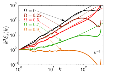
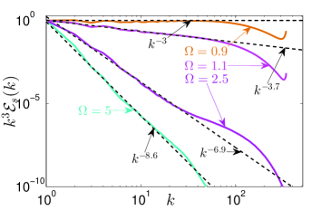
Figure 1: The normalized energy spectra ${\mathcal{E}}_{s}(k)=E(k)/E_{0}$ compensated by $k^{3}$: subcritical [Panel (a)] and supercritical [Panel (b)] (solid lines) for different values of $\Omega$. The critical spectrum (with $\Omega=0.9$) is shown in both panels. The dashed lines in Panel (a) are the LNV-prediction (3a) for the subcritical spectra with one fitting parameter in Eq.(25) ($b=0.5$) for all $\Omega<0.9$. The horizontal dashed lines in both panels show the critical spectrum. Other dashed lines in Panel (b) represent the scale-invariant spectra (16a) with an $\Omega$-dependent exponent $x$.

(a)	(b)
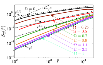
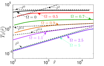
(c)	(d)

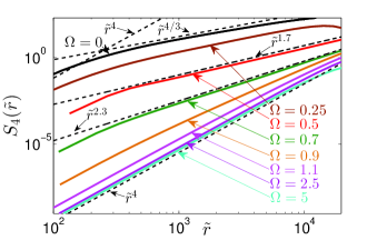
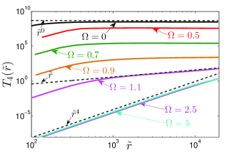
Figure 2: Color online. The second and forth-order velocity $S_{2}(\tilde{r})$ and $S_{4}(\tilde{r})$ [Panels (a),(c)] and vorticity $T_{2}(\tilde{r})$ and $T_{4}(\tilde{r})$ [Panels (b),(d)] structure functions for different $\Omega$. The straight dashed lines with the estimates of the apparent scaling exponents serve to guide the eye only.

II.2 Energy spectra

II.2.1 Critical spectrum

The numerical energy spectra are shown in Fig. 1. As was predicted in LABEL:LNV, at some particular “critical” value of the mutual friction (value of $\Omega=\Omega_{\text{cr}}$ in our current notations) there exists the self-similar balance between the energy flux and the mutual-friction energy dissipation, that leads to the scale-invariant critical spectrum $E_{\text{s}}(k)\propto k^{-3}$, Eq. (3d). As one sees in Figs. 1, the compensated spectrum for $\Omega=0.9$ is almost horizontal. Therefore, in our simulations $\Omega\approx 0.9$ corresponds to the critical spectrum.
For $\Omega<\Omega_{\text{cr}}$ we see the subcritical spectra, lying above the critical one. In this case, the energy at small $k$ is dissipated by the mutual friction and approximately $E(k)\sim k^{-3}$. For larger $k$, the $k$-independent mutual friction dissipation can be neglected compared to the energy flux (with the inverse interaction time $\gamma(k)\sim k\sqrt{kE(k)}$) and $E(k)$ can have K41 tail with the energy flux $\varepsilon_{\infty}<\varepsilon_{\text{input}}$, that for even larger $k$ is dissipated by viscosity.

II.2.2 Subcritical LNV spectra

The analytical LNV-model LNV of the subcritical spectra, based on the local in $k$-space algebraical closure (2b), was shortly presented in the Introduction. It results in Eqs. (3) for $E_{\text{cr}}(k,\Omega)$ formally without explicit fitting parameter. Nevertheless, having in mind simplification (4c) for the mutual friction, valid up to dimensionless factor of the order of unity and the uncontrolled character of Eq. (2b) for the energy flux, we replace in Eq. (3b) the numerical factor $\frac{5}{4}$ by a fitting parameter $b\approx 0.5$. Now

$$\Omega_{\text{cr}}=b\,\sqrt{k_{0}^{3}E_{0}}\ .$$ (25)

Fig. 1a compares the numerical results with the analytical LNV-spectra (3a) with $\Omega_{\text{cr}}$ given by Eq. (25).

A good agreement between DNS and analytical spectra (3a) (with $b\approx 0.5$) allows us to conclude that the algebraic LNV-model with the build-in locality of the energy transfer adequately describes the basic physical phenomena of the subcritical regime in superfluid ³He turbulence.

II.2.3 Supercritical spectra

According to LNV model LNV , for $\Omega>\tilde{\Omega}_{\text{cr}}$ we expect supercritical spectra, i.e. the energy is mainly dissipated by the mutual friction and $E_{\text{s}}(k)$ falls below the critical spectrum $k^{-3}$. As we pointed out, the energy transfer in this regime is not local anymore and a simple algebraic closure (2b) fails. Instead, we adopted an integral closure (11) and predicted the scale-invariant spectra $E_{\text{s}}(k)\propto k^{-x}$, Eq. (16a), with the exponent $x$, estimated by Eq. (16b). As we see in Fig. 1b, the supercritical energy spectra are indeed scale-invariant over more than a decade of $k$ (decaying by $13$ decades for $\Omega=5$). The scaling exponent $x$ increases with $\Omega^{\ddagger}=\Omega/\widetilde{\Omega}_{\text{cr}}$ as qualitatively predicted by Eq. (16b), although much slower. For example, $\Omega^{\ddagger}\approx 2.0$ for $\Omega=1.1$, see line (# 6) in Tab. 1. Then Eq. (16b) gives $x_{\text{model}}\simeq 5.4$ instead of numerically found $x_{\text{num}}\simeq 3.7$. This disagreement increases with $\Omega^{\ddagger}$. Here we should note that the particular form (11) of the integral closure was chosen just for simplicity. We can use much more sophisticated kind of a two-point integral closure, like EDQNM,Ors70 or Kraichnan’s Lagrangian-history direct interaction approximation Kra65 , etc. However the result will be qualitatively similar: a scale-invariant solution with the exponent $x$ that increases with $\Omega^{\ddagger}$.

We again conclude that the suggested model (now with the integral closure) describes qualitatively the physics of the supercritical regime of the superfluid ³He turbulence with the balance between the energy flux from $k\sim k_{0}$ directly to a given $k\gg k_{0}$, [the left hand side of Eq. (15)], where it is dissipated by the mutual friction [the right hand side of Eq. (15)]. This balance equation results in the power-like law $E_{\text{sp}}\propto k^{-x}$, in agreement with the DNS results. The actual value of the exponent $x$ depends on the details of the uncontrolled integral closure. A detailed analysis of the closure problem, including contribution of next order terms in perturbation approach, and comprehensive numerical simulations would be required to achieve better understanding of the statistics of the supercritical regimes of superfluid ³He turbulence

(a)	(b)
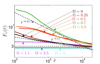
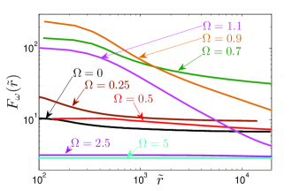
(c)	(d)

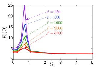
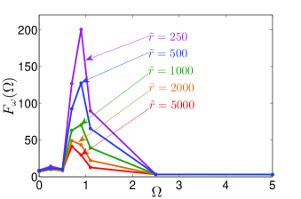
Figure 3: Color online. The velocity $F_{\text{v}}(\tilde{r})=S_{4}(\tilde{r})/S_{2}^{2}(\tilde{r})$ and vorticity $F_{\omega}(\tilde{r})=T_{4}(\tilde{r})/T_{2}^{2}(\tilde{r})$ flatness vs $\tilde{r}$ for different $\Omega$ [Panels (a) and (b)] and vs $\Omega$ for different $\tilde{r}$ [Panels (c) and (d)]. The straight dashed lines with the estimates of the apparent scaling exponents serve to guide the eye only.

II.3 Enhancement of intermittency in critical and subcritical regimes of superfluid ³He turbulence

Current Sec. II.3 is devoted to the discussion of the numerically found velocity and vorticity structure functions $S_{2}(r)$, $S_{4}(r)$ and $T_{2}(r)$, $T_{4}(r)$ and to comparison their scaling with the corresponding theoretical predictions. The most important physical observation is a significant amplification of the velocity and vorticity fluctuations in the critical and subcritical regimes (for $0.7\leq\Omega\leq 0.9$) with respect to the level typical for classical hydrodynamic turbulence. We consider this result as a manifestation of the enhancement of intermittency in superfluid ³He turbulence.

II.3.1 2${}^{\text{nd}}$-order structure functions of the velocity and vorticity $S_{2}(r)$ and $T_{2}(r)$

Consider scaling behavior of the velocity 2${}^{\text{nd}}$-order structure function $S_{2}(\tilde{r})$ for different $\Omega$, shown in Fig. 2a as a function of a dimensionless distance $\tilde{r}=r/\eta$. For the classical hydrodynamic turbulence ($\Omega=0$, black line), $S_{2}(\tilde{r})$ demonstrates the expected behavior: a viscous regime, with $S_{2}(\tilde{r})\propto\tilde{r}^{2}$ for small $r$ followed by the K41 regime, with $S_{2}(\tilde{r})\propto\tilde{r}^{\zeta_{2}}$, with $\zeta_{2}=2/3$ both shown by black dashed lines. Note, that intermittency correction to the K41 value of the scaling exponent $\zeta_{2}$ ($\zeta_{2}\approx 0.70$ instead of $\zeta_{2}=2/3\approx 0.67$) is not visible on the scale of Fig. 2a and will be discussed below. The spectrum for $\Omega=0.25$ (brown line) behaves similarly to the classical case $\Omega=0$, just with larger cross-over value of $\tilde{r}$. For larger subcritical values of $\Omega=0.5$ (red line) and $\Omega=0.7$ (green line), the viscous $S_{2}(\tilde{r})\propto\tilde{r}^{2}$ behavior for small $r$ is now followed by an apparent scaling behavior $S_{2}(\tilde{r})\propto\tilde{r}^{\zeta_{2}}$ with $\frac{2}{3}<\zeta_{2}<2$.This is a consequence of apparent scaling behavior of the subcritical LNV spectrum (3a), discussed in the Introduction. For example,for $\Omega=0.5$ $\zeta_{2}\approx 1.0$, while for $\Omega=0.7$, the apparent exponent $\zeta_{2}\approx 1.4$, and become close to $\zeta_{2}\approx 2$ already for the near critical value of $\Omega=0.9$. Note that for much larger Reynolds numbers, these apparent exponents are expected to appear only around $r_{\times}\sim 1/k_{\times}$. For $r\ll r_{\times}$ the apparent exponent should approach the classical value $\zeta_{2}=2/3$ and for $r\gg r_{\times}$ – the critical value $\zeta_{2}=1$.

As explained in Sec. I.4, in the supercritical regime, when $E_{\text{s}}(k)\propto k^{-x}$ with $x>3$, the integral (18) losses its locality and is dominated by small $r$, where the velocity field can be considered as smooth. In this regime the viscous behavior $S_{2}(\tilde{r})\propto\tilde{r}^{2}$ is expected for all $\Omega\geqslant 0.9$, as is confirmed in Fig. 2a.

Moreover, in this case the scaling behavior of the velocity structure function $S_{2}(\tilde{r})\propto\tilde{r}^{2}$ is disconnected from the energy scaling $E\propto k^{-x}$. The vorticity structure function $T_{2}(\tilde{r})$ is more informative for this regime, because, as shown in Sec. I.4, the vorticity field is not smooth for $x<5$.

Fig. 2b compares the behavior of $T_{2}(\tilde{r})$ for different $\Omega$. Consider first the test case $\Omega=0$, shown by a black line. For very small $\tilde{r}$, when $1/\tilde{r}$ exceeds viscous cutoff of the energy spectrum, we see the viscous behavior $\propto\tilde{r}^{2}$, followed by the saturation region $T_{2}(\tilde{r})\simeq$const. As explained in Sec. I.4, this is because the energy spectrum exponent $x=5/3$ is below the lower edge of the vorticity locality window (23a). For $x<3$, the integral (22) is dominated by large $k$ in the interval $\dfrac{\pi}{r}<k<k_{\text{max}}$ and $T_{2}(\tilde{r})$ becomes $r$-independent, as observed.

In Figs. 2 we present two cases with $x$ within the locality window for vorticity (23a), $3<x<5$: $\Omega=0.9$ with $x\approx 3$ and $\Omega=1.1$ with $x\approx 3.66$. According to our asymptotical (for infinitely large scaling interval) prediction (23b), we expect for these cases $z\approx 0$ and $z\approx 0.66$. The numerically found values (see Fig. 2b) are slightly larger: $z\approx 0.3$ and $z\approx 0.8$. Having relatively short scaling interval, we consider this agreement as acceptable.

For even stronger mutual friction $\Omega=2.5$ and $\Omega=5$, the energy scaling exponent $x\approx 6.9$ and $x\approx 8.6$, are above the upper edge of the vorticity locality window (23a). In this case integral (22) diverges at lower limit, giving

$$T_{2}(\tilde{r})\simeq\frac{4}{3}\,\tilde{r}^{2}\int\limits_{k_{\text{min}}}^{\infty}k^{4}E(k)\,dk\propto\tilde{r}^{2}\ .$$ (26)

as is indeed observed in Fig. 2b.

(a)	(b)	(c)
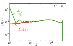
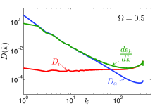
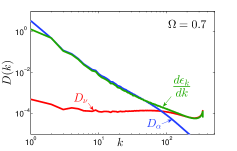
(d)	(e)	(f)

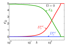
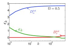
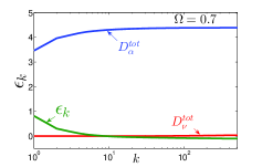
Figure 4: Color online. The differential [Panels (a),(b),(c)] and the integral [Panels (d),(e),(f)] energy balances in the subcritical regimes with $\Omega=0$ [Panels (a),(d)], $\Omega=0.5$ [Panels (b),(e)] and $\Omega=0.7$ [Panels (c),(f)]. The nonlinear energy transfer is shown by green lines, the viscous dissipation by red lines and the dissipation by mutual friction by blue lines.

II.3.2 4${}^{\text{nd}}$-order structure functions, flatnesses and enhancement of intermittency

Consider now 4${}^{\text{th}}$-order structure functions of the velocity and vorticity $S_{4}(\tilde{r})$ and $T_{4}(\tilde{r})$, shown in Fig. 2c and Fig. 2d, for the subcritical and supercritical regimes. As is well known, for the Gaussian statistics or, in a more general case, for the “mono-scaling” statistics, the fourth-order structure functions are proportional to the square of the second one: $S_{4}(\tilde{r})\propto S_{2}^{2}(\tilde{r})$ and $T_{4}(\tilde{r})\propto T_{2}^{2}(\tilde{r})$. We find such a behavior for very small $\tilde{r}$. For the classical case $\Omega=0$ (Fig. 2c) we see again scaling exponent $\zeta_{4}$ close to the standard K41 value $4/3\approx 1.33$ with intermittency corrections, hardy visible on this scale. For larger $\Omega$, the subcritical LNV spectrum (3a) becomes a superposition of two scaling laws and, as we mentioned in the Introduction, in the vicinity of a crossover wave number $k_{\times}$ may be approximated as $k^{-x}$ with an apparent scaling exponent $\frac{5}{3}<x(k)<3$. Indeed, we see in Fig. 2c that the apparent value of $\zeta_{4}$ definitely deviate from 4/3, approaching, for example, $\zeta_{4}\approx 1.7$ for $\Omega=0.5$ and $\zeta_{4}\approx 2.3$ for $\Omega=0.7$. Such a steepening of the structure functions spectra is caused by the energy dissipation by mutual friction (see Fig. 1).

More importantly, upon increase in $\Omega$ the apparent scaling of the velocity field progressively deviates from the self-similar behavior type with $S_{4}(\tilde{r})\propto S_{2}^{2}(\tilde{r})$ and $\zeta_{4}=2\zeta_{2}$. For example, for $\Omega=0.5$ $\zeta_{4}\approx 1.7<2\zeta_{2}\approx 2.0$ (such that $\xi=2\zeta_{2}-\zeta_{4}\approx 0.3$) and for $\Omega=0.7$ the difference $\xi\approx 0.5$.

To further detail this multiscaling regime, we plot in Figs. 3 the velocity and vorticity flatnesses $F_{v}(\tilde{r})$ and $F_{\omega}(\tilde{r})$, defined as:

$$F_{\text{v}}(\tilde{r})=S_{4}(\tilde{r})/S_{2}^{2}(\tilde{r})\,,\quad F_{\omega}(\tilde{r})=T_{4}(\tilde{r})/T_{2}^{2}(\tilde{r})\ .$$ (27)

For the Gaussian and mono-scaling statistics, $F_{\text{v}}(\tilde{r})$ and $F_{\omega}(\tilde{r})$ must be $\tilde{r}$-independent. In particular, for the Gaussian statistics $F_{\text{v}}(\tilde{r})=F_{\omega}(\tilde{r})$=3. As is evident in Fig. 3a and Fig. 3b, the intermittency corrections, hardly visible for structure functions for $\Omega=0$, are clearly exposed by the flatness. The velocity flatness $F_{v}(\tilde{r})$ for this case (black solid line in Fig. 3a) approximately follow the intermittent exponent for turbulence in classical fluids $\xi_{\text{cl}}\approx 0.15$, which is close to the experimental values for both the longitudinal and transversal structure functions (for previous experimental and numerical works on intermittency in the classical space-homogeneous isotropic turbulence see Refs. Gotoh02 ; Chanal00 ; Kaha98 ; Benzi10 ; Ishihara07 ; BTS-97 ) . As the mutual friction become stronger, the apparent exponent $\xi$ increases, reaching its maximum $\xi_{\text{max}}\approx 0.45\approx 3\xi_{\text{cl}}$ at $\Omega=0.7$. The vorticity flatness $F_{\omega}(\tilde{r})$[Fig. 3b] too reaches its maximum for small $\tilde{r}$ at slightly larger value of $\Omega\approx 0.9$. This is a clear evidence of significant enhancement of intermittency in the near-critical regimes of superfluid ³He turbulence.

Additional important information can be found in Figs. 3c and 3d, where $\Omega$-dependence of the velocity and vorticity flatnesses is shown for different $\tilde{r}$. The sharp peak appears for $\Omega\lesssim 0.9$. In the small $\tilde{r}$ range, the velocity flatness $F_{\text{v}}(\tilde{r})$ for $\Omega=0.7$ reaches value about 25 (compare with the Gaussian value of three and the classical hydrodynamic value about seven). At the same time the vorticity flatness reaches value of about 200, exceeding the Gaussian limit by almost two orders of magnitude.

In the supercritical regime, the intermittency sharply decreases. For example, for $\Omega>2.5$ the velocity flatness drops even below the Gaussian limit, indicating that the time dependence of the velocity becomes sub-Gaussian.

II.4 Energy balance

The direct information about the relative importance of the energy dissipation by the effective viscosity and by the mutual friction can be obtained from an analysis of the energy balance, shown in Figs. 4. The energy balance for the classical turbulence ($\Omega=0$) is presented in Fig. 4a. As expected, the energy input at a shell with a given wave number $k$, Tr$(k)=d\varepsilon(k)/dk$ (green line) is compensated by the viscous dissipation D${}_{\nu}=2\nu_{\text{s}}E_{\text{s}}(k)$ (red line). The discrepancy in the region of very small $k$ is caused by the energy pumping, which is not accounted in the balance Eq. (10a). Sometimes it is more convenient to discuss a “global” energy balance, analyzing instead of the “local” in $k$ balance Eq. (10a) its integral from $k=$ to a given $k$. In the stationary case this gives:

$$\varepsilon(k) = \varepsilon_{0}-\mbox{D}_{\nu}^{\text{tot}}(k)-\mbox{D}_{\alpha}^{\text{tot}}(k)\,,$$ (28a)

$$\mbox{D}_{\nu}^{\text{tot}}(k) = \int_{0}^{k}\mbox{D}_{\nu}(q)dq,\ \mbox{D}_{\alpha}^{\text{tot}}(k)=\int_{0}^{k}\mbox{D}_{\alpha}(q)dq\,.~{}~{}~{}~{}~{}~{}$$ (28b)

As we see in Fig. 4d (for $\Omega=0$), the energy flux over scales $\varepsilon(k)$ is almost constant up to $k\simeq 20$ and then decreases due to the viscous dissipation. Accordingly, $E_{\text{s}}(k,0)$, shown in Fig. 1a by black solid line, exhibits a K41 scaling $\propto k^{-5/3}$. Minor upward deviation from this behavior may be a numerical artifact.

The energy balance in the subcritical regime of the superfluid ³He turbulence, shown in Figs. 4b and 4e for $\Omega=0.5$ and in Figs. 4c and 4f for $\Omega=0.7$ demonstrates a qualitatively different behavior. We see in Figs. 4b and 4c that for almost all wavenumbers, the energy input Tr$(k)$ in a given $k$ (shown by green lines) is balanced by the mutual friction dissipation D${}_{\alpha}(k)$ (shown by the blue lines). Only for large $k\gtrsim 75$, the viscous dissipation begin to dominate. Nevertheless, as seen in Figs. 4e and 4f, the total contribution to the energy dissipation is dominated by the mutual friction everywhere. As expected, for larger and larger $\Omega$ the crossover wave number $k_{\times}$, at which the local dissipation by viscosity and by mutual friction are equal, increases (compare Fig. 4b with $\Omega=0.5$ and Fig. 4c with $\Omega=0.7$) and reaches $k_{\text{max}}$ for the critical regime with $\Omega=0.9$(Fig. 5a). In this case the viscous and the mutual friction dissipation become compatible only for $k\simeq k_{\text{max}}$.

In the supercritical regime, shown in Figs. 5e and 5f for $\Omega=1.1$ and $\Omega=5$, the contribution of the viscous dissipation (red lines) becomes less and less important with the increase in the supercriticality. In these cases, the nonlinear input to the energy, Tr$(k)=d\varepsilon(k)/dk$ (green lines) is fully compensated by the mutual friction dissipation(blue lines).

The global energy balance, shown in Figs. 5, confirms this physical picture.

(a)	(b)	(c)
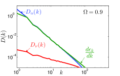
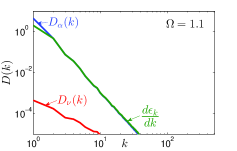
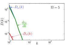
(d)	(e)	(f)

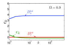
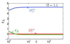
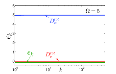
Figure 5: Color online. The differential [Panels (a),(b),(c)] and the integral [Panels (d),(e),(f)] the energy balances in the critical and the supercritical regimes with $\Omega=0.9$ [Panels (a),(d)], $\Omega=1.1$ [Panels (b),(e)] and $\Omega=5.0$ [Panels (c),(f)]. The nonlinear energy transfer is shown by green lines, the viscous dissipation by red lines and the dissipation by mutual friction by blue lines.

(a)	(b)	(c)
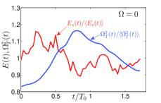
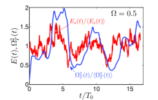
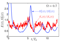
(d)	(e)	(f)

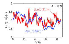
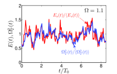
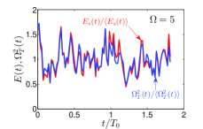
Figure 6: Color online. The energy (red lines) and enstrophy (blue lines) time evolutions in the subcritical regime normalized by mean-in-time values [Panels (a),(b),(c) with  $\Omega=0,\ 0.5,\ 0.7$], the critical [Panel (d), $\Omega=0.9$] and the supercritical regime [Panels (e),(f) with $\Omega=1.1,\ 5.0$].

II.5 Energy and enstropy time evolution

We consider here evolution of the total superfluid energy $E_{\text{s}}(t)$

$$E_{\text{s}}(t) = \int E_{\text{s}}(k,t)dk$$ (29a)

and enstrophy $1/2\Omega^{2}_{\scriptscriptstyle\rm{T}}(t)$. As expected, in the subcritical regime, when $E(k,t)$ has apparent slope $\propto k^{-x}$ with $\frac{5}{3}<x(k)<3$, the integral (29a) for total energy $E(t)$ is dominated by the small $k\sim k_{\text{min}}$, while the integral (5) for total enstropy $\Omega^{2}_{\scriptscriptstyle\rm{T}}(t)$ is dominated by the large $k\sim k_{\text{max}}$. Therefore, for the large ratio $k_{\text{max}}/k_{\text{min}}$ (in our case $k_{\text{max}}/k_{\text{min}}\sim 10^{3}$), one expects an uncorrelated behavior of $E(t)$ and $\Omega^{2}_{\scriptscriptstyle\rm{T}}(t)$ in case of a well developed turbulent cascade. This behavior is confirmed in Figs. 6a, 6b and 6c. In the supercritical regime, with the slope $x>3$, both $E(t)$ and $\Omega^{2}_{\scriptscriptstyle\rm{T}}(t)$ are dominated by the small $k\sim k_{\text{min}}$ and have to be well correlated, as is indeed seen in Figs. 6e and 6f. However, in the critical regime (Fig. 6d with $\Omega=0.9$), $E(t)$ and $\Omega^{2}_{\scriptscriptstyle\rm{T}}(t)$ are still uncorrelated because $E(t)$ is dominated by $k\sim k_{\text{min}}$, while $\Omega^{2}_{\scriptscriptstyle\rm{T}}(t)$ has equal contributions from all $k$.

II.6 Relation between $\Omega$ and temperature $T$ of possible experiments

Up to now we have considered $\Omega$ as a free parameter that determines the mutual friction by Eq. (4c), in which $\Omega_{\scriptscriptstyle\rm{T}}$ is given by Eq. (5). After the simulation with a prescribed $\Omega$ was completed, we numerically computed $\Omega_{\scriptscriptstyle\rm{T}}^{2}$, using found energy spectra and Eq. (5), see Tab.  1. Now, using Eq. (4c) we can find $\widetilde{\alpha}=\Omega/\Omega_{\scriptscriptstyle\rm{T}}$ for a given $\Omega$ in the simulations. The parameter $\widetilde{\alpha}$ in ³He strongly depend on temperature, as reported in Bevan and shown in Fig. 7. Using these data, we can find $T$ corresponding to the simulations with any prescribed $\Omega$.

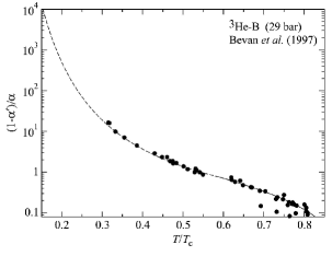
Figure 7: Temperature dependence of the mutual friction parameter $\widetilde{\alpha}(T)=\alpha/(1-\alpha^{\prime})$, taken from LABEL:Bevan

III Summary

This paper examined the basic statistical properties of the large-scale, homogeneous, steady, isotropic quantum turbulence in superfluid ³He, developing further some previous results LNV ; He3a . Direct numerical simulations of the gradually damped version of the HVBK coarse-grained two-fluid model of the superfluid He, Eqs. (4)HV ; BK ; PRB were performed using pseudo-spectral methods in a fully periodic box with a grid resolution of $N=1024^{3}$. The analytic study was based on the LNR integral closure for the energy flux LNR , Eq. (11), adapted for ³He turbulence in Eq. (I.3.2). Both the DNS and the analytic approaches do not use the assumption of locality of the energy transfer between scales. The main findings are:

1. The direct numerical simulations confirmed the previously found LNV ; He3a subcritical (3a) and critical (3d) energy spectra and showed that for $T<0.37\,T_{\text{c}}$ (see Tabl. 1) the analytic prediction are in a good quantitative agreement with the DNS results, using a single fitting parameter $b$ for all temperatures. The reason for this agreement is that in the subcritical regime the energy transfer over scales is indeed local, in accordance with the basic assumptions in Refs. LNV ; He3a . In the critical regimeLNV ; He3a with $E(k)\propto k^{-3}$, the exact locality of the energy transfer fails: all the scales contribute equally to the transfer of energy to the turbulent fluctuations with a given $k$. This leads to a logarithmic corrections to the spectrum $E(k)\propto k^{-3}$ that cannot be detected with our DNS resolution.

2. For $T>0.37\,T_{\text{c}}$, when the mutual friction exceeds some critical value, we observed in DNS and confirmed analytically the scale-invariant spectrum $E(k)\propto k^{-x}$ with a ($k$-independent) exponent $x>3$. The exponent $x$ increases gradually with the temperature, reaching in our simulation the value $x\approx 9$ for $T\approx 0.72\,T_{\text{c}}$. The reason for this behavior of the supercritical spectra with $x>3$ is that the energy is transferred directly to any given $k$ from the energy containing region at small $k$.

3. We analyzed the 2${}^{\text{nd}}$-order structure functions of the velocity and vorticity $S_{2}(r)$ and $T_{2}(r)$ and demonstrated that although their $r$-dependence can be rigorously found from the energy spectrum $E(k)$, their $r$-dependence is much less informative that the $k$-dependence of $E(k)$.

4. The 4${}^{\text{nd}}$-order structure functions of the velocity and vorticity $S_{4}(r)$ and $T_{4}(r)$ provide important additional [with respect to $E(k)$] information about the statistics of quantum turbulence in the superfluid ³He. We discover a strong enhancement of intermittency in the near-critical regimes with the level of turbulent fluctuations exceeding the corresponding level in the classical turbulence by about an order of magnitude.

5. The analysis of the energy balance and of the energy and enstrophy time evolution in various (subcritical, critical and supercritical) regimes, confirms the discovered physical picture of the quantum ³He turbulence with the local and non-local energy transfer, in which the relative importance of the energy dissipation by the effective viscosity and by the mutual friction depends in a predicted way on the temperature and the wavenumber.

We propose that these analytic and numerical findings in the description of the statistical properties of steady, homogeneous, isotropic and incompressible turbulence of superfluid ³He should serve as a basis for further studies of superfluid turbulence in more complicated or/and realistic cases: anisotropic turbulence, transient regimes, two-fluid turbulence of thermally driven counterflows in superfluid ⁴He turbulence, etc.

References

- (1) C. F. Barenghi, L. Skrbek, and K. R. Sreenivasan, Proc. Nat. Acad. Sci. USA 111, 4647-4652(2014).
- (2) C. F. Barenghi, V. S. L vovb, and P.-E. Roche, Proc. Nat. Acad. Sci. USA 111, 4683-4690(2014).
- (3) V. Eltsov, R. Hanninen, M. Krusius, Proc. Nat. Acad. Sci. USA 111,4711(2014).
- (4) S.N. Fisher, M.J. Jackson, Y.A. Sergeev, V. Tsepelin, Natl. Acad. Sci. USA 111, 4659(2014).
- (5) V. S. L’vov, S. V. Nazarenko and G. E. Volovik, JETP Letters, 80, iss.7 pp. 535-539(2004).
- (6) L. Boué, V.S. L’vov, A. Pomyalov, and I. Procaccia, Phys. Rev. B, 85 104502(2012).
- (7) V. S. L’vov, S. V. Nazarenko, O. Rudenko, Phys. Rev. B 76, 024520(2007).
- (8) U. Frisch, Turbulence: The Legacy of A. N. Kolmogorov,(Cambridge University Press, 1995 ).
- (9) L. Kovasznay, J. Aeronaut. Sci. 15, 745(1947).
- (10) L. Biferale, Annu. Rev. Fluid. Mech. 35, 441(2003).
- (11) H. E. Hall and W. F. Vinen, Proc. Roy. Soc.238, 204(1956).
- (12) I.L. Bekarevich, and I.M. Khalatnikov, Sov. Phys. JETP 13, 643 (1961).
- (13) L. Boué, V. S. L vov, Y. Nagar, S. V. Nazarenko, A. Pomyalov, and I. Procaccia, PRB 91 144501(2015).
- (14) L. Boué, V.S. L’vov, A. Pomyalov and I. Procaccia, Phys. Rev. Letts., 110, 014502(2013).
- (15) E.B. Sonin. Rev. Mod. Phys. 59, 87(1987).
- (16) A.P.Finne, T. Araki, R. Blaauwgeers, V.B. Eltsov, N.B. Kopnin, M. Krusius, L. Skrbek, M. Tsubota, and G.E. Volovik, Nature 424, 1022(2003).
- (17) V.S. L’vov and I. Procaccia, Physical Review E. 52, 3840(1995).
- (18) V.S. L’vov, I. Procaccia, Physical Review E. 52, 3858(1995).
- (19) P. A. Davidson, Y. Kaneda, K. R. Sreenivasan, Ten Chapters in Turbulence, (Cambridge University Press, 2013).
- (20) V.I. Belinicher and V.S. L’vov. Zh. Eksp. Teor. Fiz., 93, p.1269(1987). [Soviet Physics - JETP 66 pp. 303 -313 (1987) ]
- (21) D. Khomenko, V.S. L’vov, A. Pomyalov and I. Procaccia, Phys. Rev. B. 93,014516(2016).
- (22) T.D.C. Bevan, A.J. Manninen, J.B. Cook,H. Alles, J.R. Hook, and H.E. Hall, J. Low Temp. Phys. 109, 423(1997).
- (23) S. A. Orszag, J. of Fluid Mech., 41 363(1970).
- (24) R. Kraichnan, Phys. of Fluids 8, 575(1965).
- (25) T. Gotoh, D. Fukayama, T. Nakano, Phys. Fluids 14, 1065(2002).
- (26) O. Chanal, B. Chabaud, B. Castaing, B. Hébral, Eur. Phys. J. B 17, 309(2000).
- (27) H. Kahalerras, Y. Malécot, Y. Gagne, B. Castaing, Phys. Fluids 10 910(1998).
- (28) R. Benzi, L. Biferale, R. Fisher, D.Q. Lamb, F. Toschi, J. Fluid Mech. 653, 221(2010).
- (29) T. Ishihara, Y. Kaneda, M. Yokokawa, K. Itakura, A. Uno, J. Fluid Mech. 592, 335(2007).
- (30) B. Dhruva, Y. Tsuji, and K. R. Sreenivasan, Phys. Rev. E, 56, R4928(1997).