Comparison of the Iterated Equation of Motion Approach and the Density Matrix Formalism for the Quantum Rabi Model

Abstract

The density matrix formalism and the equation of motion approach are two semi-analytical methods that can be used to compute the non-equilibrium dynamics of correlated systems. While for a bilinear Hamiltonian both formalisms yield the exact result, for any non-bilinear Hamiltonian a truncation is necessary. Due to the fact that the commonly used truncation schemes differ for these two methods, the accuracy of the obtained results depends significantly on the chosen approach. In this paper, both formalisms are applied to the quantum Rabi model. This allows us to compare the approximate results and the exact dynamics of the system and enables us to discuss the accuracy of the approximations as well as the advantages and the disadvantages of both methods. It is shown to which extent the results fulfill physical requirements for the observables and which properties of the methods lead to unphysical results.

1 Introduction

In about the last 15 years, refined experimental techniques based on ultracold gases in optical lattices, created by intense laser fields grein02b ; kinos06 ; lewen07 ; bloch08 ; essli10 , have allowed for studies of closed quantum systems far away from equilibrium. Two facts are important: First, the systems must be well isolated in order not to exchange energy with the environment quickly. In this way, long observation times are possible. Second, the systems must be externally controllable in time. This is achieved by manipulating the laser fields and other external electromagnetic fields. In this way, an externally controlled $H(t)$ can be tailored to the needs of experiments which are not possible in solid state systems. One efficient way to push the system far out of equilibrium is to start from an initial quantum state which is not an eigenstate of the Hamiltonian $H(t\geq 0)$ which is constant for positive times. For instance, one may suddenly change parameters which is called a quench.

Typically, the quenched systems are in highly excited states with respect to the quenched Hamiltonian. Thus their dynamics is governed by processes on all energy scales including high energies. Properties may occur which are totally different from the equilibrium ones. This makes the field of non-equilibrium physics particularly fascinating, both, from the experimental and from the theoretical point of view. While the earlier experiments dealt with bosonic system grein02b ; kinos06 ; lewen07 ; bloch08 ; trotz12 ; ronzh13 , in the last years more and more investigations of fermionic systems are performed stroh07 ; schne08 ; stroh10 ; essli10 ; schne12 ; perto14 ; cocch16 or mixtures of both will15 . Recently, the spin degree of freedom and its correlations are also addressed lubas11 ; kosch13 ; kraus14 ; eblin14 ; brown15 ; bohne16 .

The necessity to include all energy scales makes theoretical calculations, numerical or analytical ones, challenging eiser15 . The set of tools which can be used is limited. So far, the majority of theoretical investigations were focused on one-dimensional (1D) systems, on infinite dimensional systems, and on small finite systems because for these cases powerful tools are available. For 1D systems, the tool box is best: quantum field theoretical descriptions provide analytical approaches cazal06 ; uhrig09c ; fiore10 ; sabio10 ; cazal11 ; schur12 ; rentr12 . The best understood models remain those which correspond to non-interacting fermionic or bosonic systems barth08 ; iucci10 ; calab12a ; calab12b or models which are effectively close to non-interacting ones kenne13 . Time dependent density matrix renormalization group is a powerful numerical tool which enables to study non-equilibrium phenomena in 1D systems daley04 ; white04a ; schol05 ; schol11 ; manma07 ; karra12b ; vidma13 ; zalet15 ; trotz12 ; perto14 . The other dimensionality allowing for well-controlled studies is infinite dimensions where dynamical mean-field theory becomes exact freer06 ; eckst09 ; schmi13 ; aoki14 and Gutzwiller approaches are well justified schir10 ; schir11 .

Exact diagonalization is completely flexible concerning dimensionality, but it is restricted to small systems rigol07 ; rigol08 ; torre13 . The intricate choice of basis states allows to reach even larger system size for specific issues bonca99 ; bonca07 ; mierz11a ; mierz11b ; bonca12 . Recently, the technique of exact diagonalization has been boosted by using it in a cluster approach for 1D systems rigol14 . While the results do not suffer from any finite size effects their validity is limited by the maximum extension of the clusters which can be evaluated.

A powerful macroscopic approach is to use the quantum Boltzmann equation to describe the temporal evolution of the density. This works very well for a variety of problems rapp10 ; schne12 ; eblin14 . Generically, the required scattering matrix elements are taken from leading order perturbation theory. Thus, complementary microscopic approaches are still desirable to verify the known results and to extend them to large interactions.

So far, the question to which extent conserved quantities strongly restrict or even prevent relaxation was in the center of interest rigol07 ; fiore10 ; kolla11 ; polko11 ; calab12a ; calab12b . Thus, integrable systems and systems close to integrability were studied, which drew the interest to 1D systems and to zero dimensional ones farib13a ; farib13b ; uhrig14a .

Microscopic studies of two-dimensional (2D) models out of equilibrium are still very rare; quantum Monte Carlo studies are an option goth12 . Other 2D studies address the influence of a strong electric field on the dynamics of carriers in a Mott insulator mierz11a ; mierz11b ; bonca12 . The life time of double occupancies in 2D models has been investigated experimentally and perturbatively stroh10 and by exact diagonalization lenar13 . Furthermore, the efficient representation of states as projected entangled pairs is one of the promising numerical approaches to date lubas11 ; schol11 ; orus14 . Still, the exponential growth of entanglement entropy restricts the application to short times in any dimension gober05 ; eiser15 and poses a constraint in particular in two dimensions which is not easy to overcome. Of course, three dimensional systems are even more difficult to describe reliably.

In solid state physics, pump-probe experiments provide a wealth of information on the solid systems away from equilibrium rossi02 ; matsu12 ; matsu13b ; aoki14 ; matsu16 ; ramea16 . Currently, particular interest is devoted to stirring ordered phases such as charge density waves perfe06 ; schmi08e or superconducting phases matsu12 ; matsu13b ; matsu16 ; akbar13 ; krull14 ; kempe15 ; krull16 .

The above brief review, which cannot be exhaustive, illustrates impressively that the field of non-equilibrium physics in general is currently an extremely active field of research. Thus, the development of theoretical approaches and their assessment is a timely task. To this end, we study two approaches based on the Heisenberg equations of motion and compare them in the present article. The two approaches are the density-matrix formalism (DMF) and the iterated equations of motion (iEoM), see below. They will be applied to the quantum Rabi model (QRM) which is overseeable enough to understand the origin of the observed behavior. In addition, its great advantage is that an exact solution exists which we can use to gauge the approximate approaches. Thus, the QRM provides an ideal testbed. Our study is intended to render the application of either of the approximate approaches to more complex extended models more efficiently.

The article is set up as follows. In Sect. 2, we briefly introduce the model which serves as the testbed. In Sect. 3, the two approximate approaches are introduced and their applications to the model are explained. The results are presented in Sect. 4. Finally, our findings are summarized in the Conclusions 5 where we provide an outlook as well.

2 The quantum Rabi model

The quantum Rabi model (QRM), which was introduced in 1936 by Rabi rabi36 , describes the interaction between a single bosonic mode and a two-level system. It is one of the simplest strongly coupled quantum systems. The Hamiltonian reads

$$H_{R}=\underbrace{\frac{\omega_{0}}{2}\sigma_{z}}_{H_{\sigma}}+\underbrace{\omega b^{\dagger}b}_{H_{B}}+\underbrace{g\sigma_{x}\left(b^{\dagger}+b\right)}_{H_{I}},$$ (1)

where $b^{\dagger}$ and $b$ are the bosonic creation and annihilation operators, $\omega$ the boson frequency and $\sigma_{x}$ and $\sigma_{z}$ are Pauli matrices describing the two-level system. The two-level system represented by $H_{\sigma}$ is characterized by the energy difference $\omega_{0}$. It is coupled to the bosonic environment $H_{B}$. The coupling between system and environment is described by the interaction Hamiltonian $H_{I}$ with coupling parameter $g$.

Every state of the Rabi model can be expanded in product states of a bosonic state and a spin state. In this basis, both $H_{\sigma}$ and $H_{B}$ can be chosen diagonal. However, there is no common eigenbasis for $\sigma_{x}$ and $\sigma_{z}$. Therefore, there is no common eigenbasis of all parts of the Hamiltonian. Only the total energy is preserved. We choose $\omega$ as our energy unit, i.e., all energies are given in units of $\omega$. Also, $\hbar$ is set to unity for convenience.

One key advantage of this model is that an exact solution is available. On the basis of discrete symmetries, Braak obtained an exact set of eigenstates and eigenvalues in 2011 braak11 . On this basis the numerically exact time evolution of the observables $\braket{\sigma_{x}}$ and $\braket{\sigma_{z}}$ wolf12 was computed. Another advantage of the QRM is, that the expectation values of the spin operators as well as of the number operator have to comply with certain constraints. Expectation values such as $\braket{b^{\dagger}b}$ can be rewritten according to

$$\bra{\Psi(t)}b^{\dagger}b\ket{\Psi(t)}=\left|b\ket{\Psi(t)}\right|^{2}.$$ (2)

Therefore the expectation value of the number operator remains non-negative at all times.

Every two-level system can be represented by a spin $S=\frac{1}{2}$. A maximum polarization in one direction corresponds to an expectation value 1 of the corresponding Pauli matrix. The expectation values of the Pauli matrices are bounded between -1 and 1. The number operator, the spin operators and the energy are self-adjoint operators, so their expectation values are real.

3 Methods

Here we briefly present the two general approaches used and compared in this article.

3.1 The density matrix formalism

The density matrix formalism (DMF) derives the equations of motion of expectation values by using the Heisenberg equation of motion. If the considered operators are not explicitly time dependent, but the time dependence is only induced by the Hamiltonian, the Heisenberg equation of motion reads

$$\frac{\mathrm{d}}{\mathrm{d}t}A=-i\left[A,H\right].$$ (3)

In the Heisenberg picture, the states $\ket{\Psi}$ and the corresponding density matrices $\rho_{\Psi}$ are time independent. Therefore the temporal evolution of an expectation value is given by

$$\frac{\mathrm{d}}{\mathrm{d}t}\braket{A}_{\Psi} = \frac{\mathrm{d}}{\mathrm{d}t}\mathrm{Tr}\left(\rho_{\Psi}A\right)=\mathrm{Tr}\left(\rho_{\Psi}\frac{\mathrm{d}}{\mathrm{d}t}A\right)$$ (4a)

$$= -i\mathrm{Tr}\left(\rho_{\Psi}\left[A,H\right]\right)=-i\braket{\left[A,H\right]}_{\Psi}.$$ (4b)

Depending on the Hamiltonian, calculating the commutator of the operator $A$ and the Hamiltonian may (and generically will) result in the appearance of additional expectation values whose temporal evolutions have to be calculated again by applying equation (4). In case of a bilinear fermionic or bosonic Hamiltonian, this procedure results in a closed set of differential equations that can be computed exactly. But in the case of interacting Hamiltonians, for instance the QRM, the application of (4) leads to an infinite hierarchy of differential equations which does not close. Hence, these equations cannot be integrated straightforwardly.

A truncation is necessary in order to obtain a closed system so that the temporal evolution of expectation values can be computed. One way to truncate is to neglect the interaction between operators if the corresponding cumulant exceeds a certain order. The order of the cumulant is given by the number of operators appearing in it kubo62 ; fulde88 . The fundamental idea of the DMF is that the contribution of the cumulant including a larger number of operators, i.e., being of higher order, is smaller.

Cumulants occur upon factorizing the expectation value of an operator product kubo62 . They are calculated according to

$$\braket{A_{1}^{\alpha}...A_{n}^{\beta}}^{c}=\left.\frac{\partial^{\alpha}}{\partial\lambda_{1}^{\alpha}}...\frac{\partial^{\beta}}{\partial\lambda_{n}^{\beta}}\ln\left\langle\prod_{i=1}^{n}e^{\lambda_{i}A_{i}}\right\rangle\right|_{\lambda_{1}=...=\lambda_{n}=0}$$ (5)

and comprise the dynamics of the interaction between the operators in the initial product. For instance, the cumulants for expectation values consisting of one, two and three operators are given by

$$\braket{A}^{c} = \braket{A}$$ (6a)

$$\braket{AB}^{c} = \braket{AB}-\braket{A}\braket{B}$$ (6b)

$$\braket{ABC}^{c} = \braket{ABC}+2\braket{A}\braket{B}\braket{C}$$ (6c)

$$-\braket{A}\braket{BC}-\braket{B}\braket{AC}-\braket{C}\braket{AB}.$$

The number $n$ in (5) denotes the order of the cumulant, i.e., the number of operators occuring in it.

To construct the truncation by cumulants, the system of differential equations for the expectation values has to be converted into a system of differential equations for the corresponding cumulants. For instance, the temporal evolution of $\braket{\sigma_{z}b}$ can be expressed in cumulants according to

$$\frac{\mathrm{d}}{\mathrm{d}t}\braket{\sigma_{z}b} = -i\omega\braket{\sigma_{z}b}+g\braket{\sigma_{y}}$$ (7b)

$$+2g\braket{\sigma_{y}bb}+2g\braket{\sigma_{y}b^{\dagger}b}$$

$$= -i\omega\braket{\sigma_{z}b}^{c}-i\omega\braket{\sigma_{z}}\braket{b}+g\braket{\sigma_{y}}$$

$$+2g\left(\braket{\sigma_{y}b}^{c}\braket{b}+\braket{\sigma_{y}b}^{c}\braket{b}+\braket{bb}^{c}\braket{\sigma_{y}}\right)$$

$$+2g\left(\braket{\sigma_{y}b}^{c}\braket{b^{\dagger}}+\braket{\sigma_{y}b^{\dagger}}^{c}\braket{b}+\braket{b^{\dagger}b}^{c}\braket{\sigma_{y}}\right)$$

$$+2g\left(\braket{\sigma_{y}}\braket{b}\braket{b}+\braket{\sigma_{y}}\braket{b^{\dagger}}\braket{b}\right)$$

$$+2g\left({\braket{\sigma_{y}b^{\dagger}b}^{c}}+\braket{\sigma_{y}bb}^{c}\right).$$

Furthermore, using the product rule for calculating the derivative with respect to the time leads to

$$\frac{\mathrm{d}}{\mathrm{d}t}\braket{\sigma_{z}b} = \left(\frac{\mathrm{d}}{\mathrm{d}t}\braket{\sigma_{z}b}^{c}\right)$$ (8b)

$$+\braket{\sigma_{z}}^{c}\left(\frac{\mathrm{d}}{\mathrm{d}t}\braket{b}^{c}\right)+\braket{b}^{c}\left(\frac{\mathrm{d}}{\mathrm{d}t}\braket{\sigma_{z}}^{c}\right)$$

$$= \left(\frac{\mathrm{d}}{\mathrm{d}t}\braket{\sigma_{z}b}^{c}\right)-i\omega\braket{b}\braket{\sigma_{z}}-ig\braket{\sigma_{x}}\braket{\sigma_{z}}$$

$$+2g\left(\braket{\sigma_{y}b}^{c}\braket{b}+\braket{\sigma_{y}b^{\dagger}}^{c}\braket{b}\right)$$

$$+2g\left(\braket{\sigma_{y}}\braket{b}\braket{b}+\braket{\sigma_{y}}\braket{b^{\dagger}}\braket{b}\right).$$

Equating (7b) and (8b) yields the differential equation for the cumulant

$$\frac{\mathrm{d}}{\mathrm{d}t}\braket{\sigma_{z}b}^{c}= - i\omega\braket{\sigma_{z}b}^{c}-ig\braket{\sigma_{x}}\braket{\sigma_{z}}$$

$$+ g\braket{\sigma_{y}}$$

$$+ 2g\left({\color[rgb]{1,0,0}\braket{\sigma_{y}bb}^{c}}+\braket{\sigma_{y}b}^{c}\braket{b}+\braket{bb}^{c}\braket{\sigma_{y}}\right)$$

$$+ 2g\left({\color[rgb]{1,0,0}\braket{\sigma_{y}b^{\dagger}b}^{c}}+\braket{\sigma_{y}b}^{c}\braket{b^{\dagger}}+\braket{b^{\dagger}b}^{c}\braket{\sigma_{y}}\right).$$

The cumulants marked in red (dark grey) are of third order because the number of operators involved in the cumulant is three. Thus, these cumulants are truncated in an approximation of second order. We emphasize that this is not equivalent to a perturbative truncation in the order of the coupling parameter $g$. The truncation based on the order of cumulants only requires the assumption that the contribution of a cumulant decreases with the number of operators involved. This leads to a closed system of differential equations amenable to numerical solution.

3.2 The iterated equation of motion approach

Similar to the DMF, the approach of iterated equations of motion (iEoM) is based on the Heisenberg equation of motion. But instead of directly deriving the temporal evolution of certain expectation values, the temporal evolution of certain operators is computed uhrig09c ; hamer13a ; hamer13b ; hamer14a ; krull15a . As in the DMF, the commutator in the Heisenberg equation of motion leads to an infinite hierarchy of differential equations for generic Hamiltonians. Thus, in order to solve for the temporal evolution of the operators, a truncation becomes necessary. To this end, we start from an operator basis for which we solve the iEoM. The basic idea is that the approximation becomes more and more accurate upon extending this basis.

Such an operator basis can be obtained by systematically extending the ansatz for each initial operator or by defining a common operator basis for all operators under study. The time dependences of the operators in the Heisenberg picture being elements of the chosen basis are put into prefactors $\gamma_{nl}(t)$ of the time independent operators $V_{n}^{S}$ in the Schrödinger picture. Hence, the ansatz for the dynamics of an operator $V_{n}^{H}$ in the Heisenberg picture is given by

$$V_{i}^{H}(t)=\sum_{l}\gamma_{nl}(t)V_{l}^{S}.$$ (10)

The initial conditions of the prefactors are

$$\gamma_{nl}(t=0)=\begin{cases}1&\text{for }l=n\\ 0&\text{for }l\neq n\end{cases}.$$ (11)

As mentioned above, the operator basis can be obtained by initially only considering the operator $V_{n}$ and extending the basis systematically by operators $V_{\text{new}}$ occurring in the commutator in Eq. (3). The resulting differential equations can be truncated strictly in the order of the coupling parameter $g$ by including only operators of $\mathcal{O}(g^{n})$ in the operator basis.

The alternative approach is to define a common operator basis for all operators. If such a common operator basis is defined beforehand the truncation is not applied in a strict order of the coupling parameter $g$. Contributions of $\mathcal{O}(g^{n+m})$ are included if the corresponding operator is an element of the chosen basis. Thus, the results obtained by truncating using an operator basis will differ from the results obtained by truncating strictly in the order of the coupling parameter.

For instance, the initial ansatz for the annihilation operator is given by

$$b^{H}(t)=\beta_{0}(t)b^{S}.$$ (12)

Heisenberg’s equation of motion implies

$$\frac{\mathrm{d}}{\mathrm{d}t}b(t)=\beta_{0}\left(-i\left[b,H_{R}\right]\right)=\beta_{0}\left(-i\omega b-ig\sigma_{x}\right),$$ (13)

so $\sigma_{x}$ is included in the extended ansatz which now reads

$$b(t)=\beta_{0}(t)b+g\beta_{1}(t)\sigma_{x}.$$ (14)

This can again be computed using the Heisenberg equation of motion. Extending the ansatz systematically and only considering contributions in $\mathcal{O}(g^{1})$ eventually leads to

$$b(t)=\beta_{0}(t)b+g\beta_{1}(t)\sigma_{x}+g\beta_{2}(t)\sigma_{y},$$ (15)

so that the temporal evolution of the annihilation operator is given both by

$$\frac{\mathrm{d}}{\mathrm{d}t}b(t) = \beta_{0}\left(-i\omega b-ig\sigma_{x}\right)+g\beta_{1}\left(-\omega_{0}\sigma_{y}\right)$$

$$+g\beta_{2}\left(\omega_{0}\sigma_{x}\right)$$

$$= b\left(-i\omega\beta_{0}\right)+g\sigma_{x}\left(-i\beta_{0}+\omega_{0}\beta_{2}\right)$$

$$+g\sigma_{y}\left(-\omega_{0}\beta_{1}\right)$$

and by

$$\frac{\mathrm{d}}{\mathrm{d}t}b(t)=b\frac{\mathrm{d}}{\mathrm{d}t}\beta_{0}+g\sigma_{x}\frac{\mathrm{d}}{\mathrm{d}t}\beta_{1}+g\sigma_{y}\frac{\mathrm{d}}{\mathrm{d}t}\beta_{2}.$$ (17)

Comparing Eqs. (16) and (17) yields the closed system of differential equations

$$\frac{\mathrm{d}}{\mathrm{d}t}\beta_{0} = -i\omega\beta_{0}$$ (18a)

$$\frac{\mathrm{d}}{\mathrm{d}t}\beta_{1} = -i\beta_{0}+\omega_{0}\beta_{2}$$ (18b)

$$\frac{\mathrm{d}}{\mathrm{d}t}\beta_{2} = -\omega_{0}\beta_{1},$$ (18c)

which can be solved numerically. In this case, truncating strictly in the coupling parameter $g$ and truncating according to the operator basis yields the same result. But if contributions in $\mathcal{O}(g^{2})$ are considered, computing Heisenberg’s equation of motion for the ansatz

$$b(t)=\beta_{0}(t)b+g\beta_{1}(t)\sigma_{x}+g\beta_{2}(t){\color[rgb]{0,1,0}{\sigma_{y}}}$$ (19)

$$+g^{2}\beta_{3}(t)\sigma_{z}b+g^{2}\beta_{4}(t)\sigma_{z}b^{\dagger}$$

leads to

$$\frac{\mathrm{d}}{\mathrm{d}t}b(t) = \beta_{0}\left(-i\omega b-ig\sigma_{x}\right)$$

$$+g\beta_{1}\left(-\omega_{0}\sigma_{y}\right)+g\beta_{2}\left(\omega_{0}\sigma_{x}-2g\sigma_{z}b-2g\sigma_{z}b^{\dagger}\right)$$

$$+g^{2}\beta_{3}\left(-i\omega\sigma_{z}b+{\color[rgb]{0,1,0}{g\sigma_{y}}}+{\color[rgb]{1,0,0}{2g\sigma_{y}bb+2g\sigma_{y}b^{\dagger}b}}\right)$$

$$+g^{2}\beta_{4}\left(i\omega\sigma_{z}b^{\dagger}+{\color[rgb]{0,1,0}{g\sigma_{y}}}+{\color[rgb]{1,0,0}{2g\sigma_{y}b^{\dagger}b^{\dagger}+2g\sigma_{y}b^{\dagger}b}}\right).$$

In a strict truncation in $\mathcal{O}(g^{2})$, both the operators highlighted in green (light grey) and in red (dark grey) are neglected. This differs from the truncation in the more general approach based on a pre-defined operator basis. Using the pre-defined operator basis the green (light grey) contributions in $\mathcal{O}(g^{3})$ are kept because $\sigma_{y}$, which can be found in the ansatz (19), is an element of the operator basis.

The definition of a common operator basis for all operators allows us to describe the dynamics of the operators in matrix notation. The temporal evolution of an operator that is not explicitly time dependent is given by

$$\frac{\mathrm{d}}{\mathrm{d}t}V_{n}=i\left[V_{n},H\right]=i\sum_{j}M_{nj}V_{j}.$$ (21)

The dynamics of the vector $\vec{V}$ containing all operators in the basis can therefore be described using the matrix $\uuline{M}$ according to

$$\frac{\mathrm{d}}{\mathrm{d}t}\vec{V}^{H}=i\uuline{M}\vec{V}^{H}.$$ (22)

Henceforth, we will call the transposed matrix $\uuline{M}^{T}$ the dynamic matrix belonging to the chosen basis of operators. The Hamiltonian $H_{R}$ is not time dependent and thus equal in both the Schrödinger and the Heisenberg picture. The Heisenberg equation of motion can be written as

$$i\left[V_{n}^{H},H\right] = -i\left[\sum_{j}\gamma_{nj}V_{j}^{S},H\right]$$ (23a)

$$= \sum_{j}\gamma_{nj}\left(-i\left[V_{j}^{S},H\right]\right)$$ (23b)

$$= i\sum_{j}\gamma_{nj}\sum_{k}M_{jk}V_{k}^{S}$$ (23c)

$$= i\sum_{k}V_{k}^{S}\sum_{j}\gamma_{nj}M_{jk}.$$ (23d)

Using (10), the commutator yields

$$i\left[V^{H}_{n},H\right]=\frac{\mathrm{d}}{\mathrm{d}t}V^{H}_{n}=\sum_{k}V_{k}^{S}\frac{\mathrm{d}}{\mathrm{d}t}\gamma_{nk}.$$ (24)

Comparing Eqs. (23d) and (24) we obtain

$$\frac{\mathrm{d}}{\mathrm{d}t}\gamma_{nk} = i\sum_{j}\gamma_{nj}M_{jk}$$ (25a)

$$\frac{\mathrm{d}}{\mathrm{d}t}\uuline{\gamma} = i\uuline{\gamma}\uuline{M},$$ (25b)

where the latter notation underlines the matrix form of the equation. Both $\uuline{\gamma}$ and $\uuline{M}$ are quadratic matrices. Eq. (25b) is equivalent to the vector equation

$$\frac{\mathrm{d}}{\mathrm{d}t}\left(\vec{\gamma}_{n}\right)^{T}=i\left(\vec{\gamma}_{n}\right)^{T}\uuline{M}.$$ (26)

Here, $\vec{\gamma}_{n}$ is a column vector made from the elements of the $n$-th row of the matrix $\uuline{\gamma}$. Transposing (26) leads to the vectorial differential equation

$$\frac{\mathrm{d}}{\mathrm{d}t}\vec{\gamma}_{n}=i\uuline{M}^{T}\vec{\gamma}_{n},$$ (27)

that is solved by

$$\vec{\gamma}_{n}=\sum_{m}C_{nm}e^{i\lambda_{m}t}\vec{u}_{m}.$$ (28)

Here, $\lambda_{m}$ denotes the eigenvalues and $\vec{u}_{m}$ the eigenvectors of the dynamic matrix $\uuline{M}^{T}$. Therefore, choosing an operator basis that corresponds to a hermitian matrix $\uuline{M}$ guarantees that the temporal evolution consists of oscillatory contributions only as is physically reasonable in quantum mechanics. No exponentially diverging time dependence can occur. Conversely, if the dynamic matrix $\uuline{M}^{T}$ is not hermitian complex eigenvalues may appear which imply exponentially diverging contributions which are unphysical.

For the QRM no operator basis can be found that implies a hermitian dynamic matrix $\uuline{M}^{T}$ and comprises all operators in $\mathcal{O}(g^{2})$. But there is a basis that leads to a matrix with only real eigenvalues satisfying exactness in $\mathcal{O}(g^{3})$. This basis will be discussed more specifically in the following section.

We stress an inherent advantage of the iEoM approach, namely that the non-negativity of the number operator is guaranteed. Calculating the temporal evolution of $b(t)$ the number operator can be expressed by $b^{\dagger}(t)b(t)$ which is a non-negative operator by construction. Thus, the resulting expectation values will always be non-negative as it has to be on physical grounds.

4 Results

The systems of differential equations for both the DMF and the iEoM approach are solved numerically using the Livermore Solver for Ordinary Differential Equations radha93 or, alternatively, a Runge Kutta algorithm of fourth order dorma86 . The system of differential equations for the DMF cannot be integrated for long time intervals with either of these algorithms because the numerically iterated matrix of coefficients becomes singular within machine precision.

The energy splitting of the spin $\omega_{0}$ used below in the computations of the temporal evolutions of the expectation values is $\omega_{0}=0.5\omega$. This value is chosen because it was also used in the exact data provided in Ref. wolf12 . For the iEoM, two different operator bases are considered. Both comprise the elementary set of operators

$$V := \left\{\sigma_{x},\,\sigma_{y},\,\sigma_{z}\right\}$$

$$\cup\left\{\sqrt{2}\sigma_{x}b,\,\sqrt{2}\sigma_{y}b,\,\sqrt{2}\sigma_{z}b\,\right\}$$

$$\cup\left\{\sqrt{2}\sigma_{x}b^{\dagger},\,\sqrt{2}\sigma_{y}b^{\dagger},\,\sqrt{2}\sigma_{z}b^{\dagger}\right\}$$

$$\cup\left\{\sqrt{2}\sigma_{x}bb,\,\sqrt{2}\sigma_{y}bb,\,\sqrt{2}\sigma_{z}bb,\,\right\}$$

$$\cup\left\{\sqrt{2}\sigma_{x}b^{\dagger}b^{\dagger},\,\sqrt{2}\sigma_{y}b^{\dagger}b^{\dagger},\,\sqrt{2}\sigma_{z}b^{\dagger}b^{\dagger}\right\}$$

$$\cup\left\{2\sigma_{x}b^{\dagger}b,\,2\sigma_{y}b^{\dagger}b,\,2\sigma_{z}b^{\dagger}b\right\}\,,$$

where the pre-factors are chosen such that the ensuing dynamic matrix $\uuline{M}^{T}$ is hermitian. However, the basis $V$ is not sufficient to describe the QRM because $H_{B}$ in (1) contains the bosonic operators without spin operators attached but neither $b^{\dagger}b$, nor $b$ or $b^{\dagger}$ are elements of $V$. Thus, we consider two extensions

$$V_{\mathrm{sep}} := V\cup\left\{\mathbbm{1},\,b,\,b^{\dagger}\right\}$$ (30a)

$$V_{\mathrm{prod}} := V\cup\left\{\mathbbm{1},\,\sqrt{2}b^{\dagger}b\right\}.$$ (30b)

The difference between both bases is that one ($V_{\mathrm{prod}}$) contains $b^{\dagger}b$ in a product while the other ($V_{\mathrm{sep}}$) contains the bosonic creation and annihilation operator separately.

While none of the two operator bases leads to a hermitian dynamic matrix $\uuline{M}^{T}$, we find that the matrix resulting from $V_{\mathrm{prod}}$ only has real eigenvalues. Therefore, no exponential divergences occur if this basis is used to calculate the expectation values. In contrast, the matrix resulting from $V_{\mathrm{sep}}$ has complex eigenvalues occurring in conjugate pairs with finite imaginary parts. This implies that exponentially diverging solutions for the expectation values occur. Independent from the divergence behavior the expectation value $\langle b^{\dagger}b\rangle(t)$ remains non-negative at all times.

4.1 Temporal evolution of the spin operators

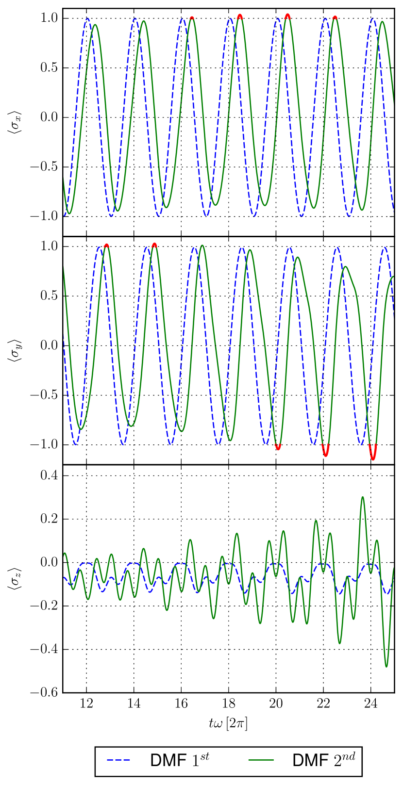
Figure 1: DMF results for the temporal evolution of the expectation values of the spin operators starting from $\braket{\sigma_{x}}(0)=1$, $\omega_{0}=0.5\omega$, and $g=0.1\omega$ in first and second order. Expectation values with $|\braket{\sigma}|>1$ in second order are marked in red.

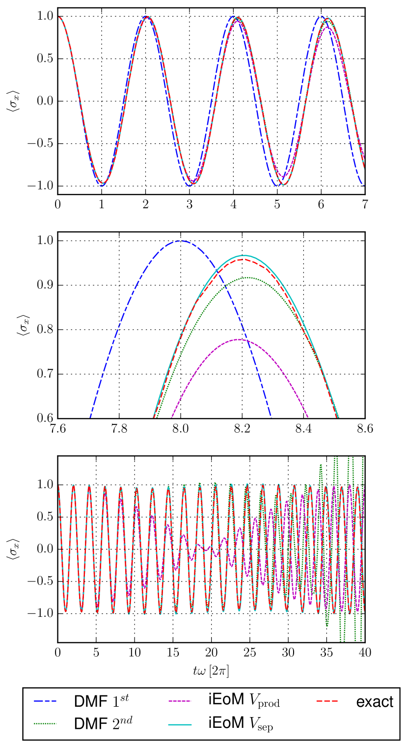
Figure 2: Results for the temporal evolution of $\braket{\sigma_{x}}$ starting from $\braket{\sigma_{x}}(0)=1$, $\omega_{0}=0.5\omega$, and $g=0.1\omega$, computed using the DMF in first and second order as well as the iEoM for $V_{\mathrm{prod}}$ and $V_{\mathrm{sep}}$. To show the agreement with the exact solution, three different time ranges are displayed. Because the first order results in the DFM differ significantly from the exact solution even on short time scales, they are not displayed in the lowest panel.

Due to the truncation, the DMF approach may lead to unphysical behaviour, for instance the expectation values for the spin operators can have absolute values beyond unity or the expectation value for the particle number turns negative. The QRM is an excellent testbed to study and to analyze such behavior. Fig. 1 shows the DMF results for the temporal evolution of the spin operators in first and second order for $g=0.1\omega$, where the initial state is set to

$$\ket{\Psi_{0}}=\ket{\chi}\otimes\ket{0},$$ (31)

that is to say that the spin is polarized in $x$-direction and the bosonic mode is initially unoccupied. In first order, where the iEoM and the DMF approach produce the same results, $\braket{\sigma_{x}}$ and $\braket{\sigma_{y}}$ oscillate with a constant phase shift of $\frac{\pi}{2}$. This corresponds to a rotation in the $xy$-plane as expected for a precessing spin (Larmor precession). Inspecting the second order results of the DMF, it becomes evident that for $t\omega[2\pi]>12.5$ the absolute expectation values of the Pauli matrices exceed unity which clearly is unphysical.

Fig. 2 displays the results of the DMF in comparison to the exact solution from Ref. wolf12 and to the results of the iEoM using the operator bases $V_{\mathrm{prod}}$ and $V_{\mathrm{sep}}$. It should be noted that calculating the temporal evolution of the spin operators using the iEoM, a strict truncation in second order of the coupling parameter equals a truncation using the operator basis $V_{\mathrm{prod}}$.

Looking at short times, it is obvious that the DMF results in first order differ significantly from the exact solution in both amplitude and phase. But the second order DMF results agree better with the exact solution than the results of the iEoM using $V_{\mathrm{prod}}$. At the same time, the temporal evolution computed using the iEoM based on $V_{\mathrm{sep}}$ is in remarkable agreement with the exact evolution. To illustrate this good agreement, a zoom of the peak of the temporal evolution around $t\omega=2\pi\cdot 8.2$ is displayed in the middle panel in Fig. 2. This excellent agreement persists for longer times as displayed in the lower panel. In addition, the lower panel shows that the expectation value computed using second order DMF diverges exponentially which is a serious caveat physically. In contrast, the results of the iEoM using $V_{\mathrm{prod}}$ show no unphysical behavior and no exponential divergences. This remains true for larger coupling parameters and was to be expected because the dynamic matrix $\uuline{M}^{T}$ resulting from $V_{\mathrm{prod}}$ only has real eigenvalues.

But the iEoM approach based on $V_{\mathrm{prod}}$ leads to large discrepancies to the exact solution. It is remarkable that the analytically better justified ansatz leads to qualitatively worse results. While the computation using $V_{\mathrm{sep}}$ implying complex eigenvalues agrees significantly better, the expectation values of the spin operators show unphysical results exceeding unity, even though no divergences occur on the considered time scales. Because the deviations of the results computed using the DMF in $\text{1}^{\text{st}}$ order become evident on short time scales, these results are not displayed for larger time scales in the lowest panel.

We depict only the temporal evolution of $\braket{\sigma_{x}}$, but the computation of $\braket{\sigma_{z}}$ yields similar results when using $V_{\mathrm{prod}}$ and $V_{\mathrm{sep}}$. This is due to the block structure of the dynamic matrix $\uuline{M}^{T}$ in (27). There are submatrices which are not linked to the other blocks so that the dynamics of certain operators is not coupled to the other operators in the operator basis. This means that for certain initial conditions reduced bases $V_{\mathrm{red}}$ can be identified yielding the same temporal evolution as the compuation in the full basis.

In concrete terms, neither the coefficients corresponding to $b$ and $b^{\dagger}$ nor the coefficient belonging to the number operator appear in the evolution of $\sigma_{z}$. Hence, the reduced basis

$$V_{\mathrm{red}} := \left\{\sigma_{z},\,\mathbbm{1}\right\}$$

$$\cup\left\{\sqrt{2}\sigma_{x}b,\,\sqrt{2}\sigma_{x}b^{\dagger}\,\right\}$$

$$\cup\left\{\sqrt{2}\sigma_{y}b,\,\sqrt{2}\sigma_{y}b^{\dagger}\right\}$$

$$\cup\left\{\sqrt{2}\sigma_{z}bb,\,\sqrt{2}\sigma_{z}b^{\dagger}b^{\dagger},\,2\sigma_{z}b^{\dagger}b\right\}$$

is sufficient and the corresponding dynamic matrix is hermitian. Therefore, the results for the temporal evolution of $\braket{\sigma_{z}}$ agree almost perfectly with the exact temporal evolution for small coupling parameters and even for larger coupling parameters no unphysical behavior is observed.

4.2 Temporal evolution of the particle number operator and the expectation value of energy

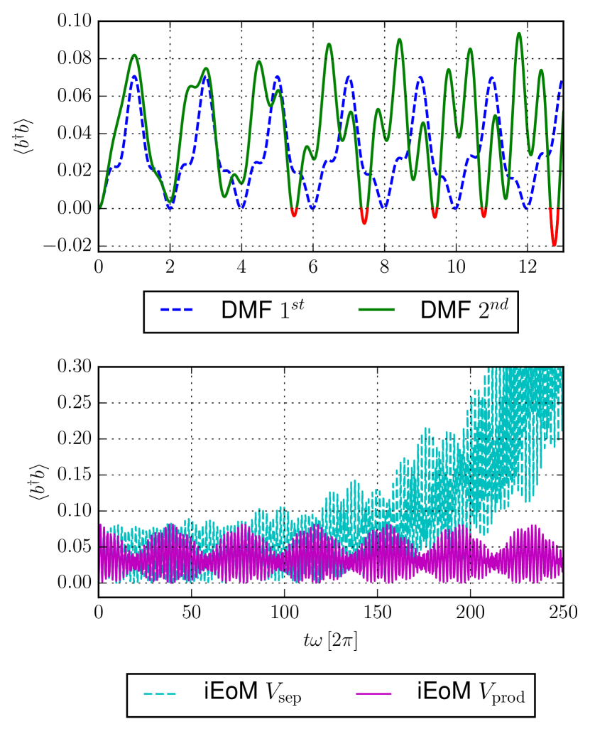
Figure 3: Results for the temporal evolution of the number operator for the parameters $\braket{\sigma_{x}}(0)=1$, $\omega_{0}=0.5\omega$, and $g=0.1\omega$. The upper panel displays the DMF results obtained in first and second order. Expectation values with $\braket{b^{\dagger}b}<0$ occurring in second order are marked in red. The lower panel displays the iEoM results based on $V_{\mathrm{prod}}$ and on $V_{\mathrm{sep}}$ on a large time scale.

The main advantage of the iEoM over the DMF is that products of operators with their hermitian conjugates will yield non-negative results by construction. By this argument, the operator basis $V_{\mathrm{sep}}$ comprising $b$ as well as $b^{\dagger}$ guarantees a non-negative temporal evolution of the number operator. We observe, however, that the expectation values of the number operator $b^{\dagger}b$ computed in the operator basis $V_{\mathrm{prod}}$ does not display negative values either. So these results are physically reasonable. But at present, we do not see a compelling mathematical argument why this is so.

In the upper panel of Fig. 3 it is evident, that the DMF results in second order display unphysical behavior, namely particle densities falling below zero, even for short times. These negative expectation values are highlighted in red. By contrast, the expectation value of the number operator remains non-negative for all times within the iEoM approach.

While the expectation value computed using $V_{\mathrm{prod}}$ shows regular oscillations and does not exceed a maximum value the expectation value computed using $V_{\mathrm{sep}}$ diverges exponentially. This must be classified unphysical since the full quantum mechanical dynamics is unitary and thus cannot yield diverging results. For instance, the expectation value of the total energy has to stay constant.

Computing the expectation value of the energy using the iEoM, it is important to calculate the expectation value $\braket{H_{\text{I}}}=g\braket{\sigma_{x}\left(b+b^{\dagger}\right)}$ using the evolution of $\sigma_{x}b$ and $\sigma_{x}b^{\dagger}$ which are elements of both operator bases. Using the product of the temporal evolutions of $\sigma_{x}$ and $b$ or $b^{\dagger}$ computed separately, the argument implicitly assumes that $\left[\sigma_{i},b^{\mu}\right]=0$. But this does not hold true for the truncated temporal evolutions of the operators except at $t=0$ for trivial reason. Therefore, the expectation value $\braket{\sigma_{x}(t)\left(b(t)+b^{\dagger}(t)\right)}$ computed from the product has a non-negligible imaginary part even though the operator is hermitian. By contrast, the expectation value computed using $\sigma_{x}b(t)$ and $\sigma_{x}b^{\dagger}(t)$ remains real for all times as it has to be.

The temporal evolution of the expectation value of energy is displayed in Fig. 4. As expected, the evolution computed using $V_{\mathrm{sep}}$ diverges. This divergence is solely due to the contribution of the number operator to $\braket{H_{\text{R}}}$, as the temporal evolution of $\braket{\sigma_{x}b}$ is the same for $V_{\mathrm{sep}}$ and for $V_{\mathrm{prod}}$.

Nevertheless, since all calculations are exact in second order in $g$, no matter if they are based on $V_{\mathrm{sep}}$ or on $V_{\mathrm{prod}}$, the error of $\braket{H_{\text{R}}}$ is of order $g^{3}$ or possibly of higher order. The plot of the deviation of $\braket{H_{\text{R}}}$ from zero on a double logarithmic scale reveals that for small couplings the proportionality $\braket{H_{\text{R}}}\propto g^{4}$ holds true. This behavior agrees with our expectation because $H_{\text{R}}$ is invariant under the transformation

$$g \leftrightarrow -g$$ (33a)

$$b \leftrightarrow -b\,,$$ (33b)

which implies that the ground state energy and certain other expectation values only depend on even powers of $g$. Thus, the accuracy of the energy in order $g^{3}$ implies the accuracy in order $g^{4}$.

Note that $V_{\mathrm{sep}}$ is the operator basis that leads to a significantly better agreement with the exact results for the temporal evolution of the spin operators, in spite of the detrimental long time behavior discernible in Fig. 4. Contrary to the energy computed using $V_{\mathrm{sep}}$, the energy using $V_{\mathrm{prod}}$ does not diverge. Here, the expectation value oscillates around zero and shows beating behavior with a constant amplitude for all times. So again, we observe that the conceptually more suitable operator basis leads to results that deviate more from the exact solution for intermediate times.

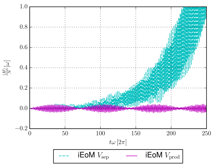
Figure 4: iEoM results for the temporal evolution of the expectation value of the energy for $\braket{\sigma_{x}}(0)=1$, $\omega_{0}=0.5\omega$, and $g=0.1\omega$ using the operator bases $V_{\mathrm{prod}}$ and $V_{\mathrm{sep}}$.

5 Conclusions and Outlook

5.1 Objective

We studied the real time behavior in the quantum Rabi model (QRM) off equilibrium by two related, but distinct approximate approaches. The QRM is chosen because it represents a correlated non-trivial model for which an exact solution for the non-equilibrium dynamics exists braak11 ; wolf12 .

Both approximate approaches to be compared are based on the Heisenberg equations of motion. The first approach is the widely used density-matrix formalism (DMF) which directly focuses on the time dependence of expectation values rossi02 ; akbar13 ; krull14 ; krull16 . The second approach is dubbed iterated equations of motion (iEoM) and focuses on the time evolution of the operators described in a basis of time independent operators uhrig09c . The motivation is to study how well these approaches work and to judge their strengths and weaknesses. This will help to employ them for other systems more efficiently.

5.2 Summary

We found that the DMF applied to the QRM in second order leads to non-physical results. The expectation values of the non-negative number operator turn spuriously negative. Furthermore, significant deviations from the exact solution occur.

The iEoM approach requires to work with an operator basis chosen beforehand. Different choices of this basis lead to different dynamic matrices and thus to different results. A key advantage of the iEoM approach is that densities stay non-negative by construction as it has to be.

Conceptually, the dynamic matrices describing the operator dynamics in the iEoM should have only real eigenvalues because only real frequencies guarantee solutions of merely oscillatory character avoiding exponential divergences. It is such oscillatory behavior which is characteristic for unitary quantum dynamics. This is ensured formally for hermitian dynamic matrices.

For the QRM, an operator basis ($V_{\text{sep}}$) comprising both $b$ and $b^{\dagger}$ leads to a dynamic matrix with complex eigenvalues. Still, non-negative expectation values for the number operator are guaranteed. The complex eigenvalues, however, imply that the expectation values of the number operator show exponential divergence. In addition, unphysical results occur for the expectation values of the spin operators for longer times.

An alternative operator basis ($V_{\text{prod}}$) avoiding the single operators $b$ and $b^{\dagger}$ but including the product $b^{\dagger}b$ leads to a dynamic matrix with only real eigen values. Here, no unphysical results or divergences occur. The number operator remains non-negative, even though this is not guaranteed by construction. Therefore, this is the basis of choice on conceptual grounds.

But we observe that the former choice of basis agrees significantly better than the latter choice in spite of the conceptual assets of the latter. At first sight, this appears astonishing. At second thought, however, the explanation is that it is strongly advantageous to include the fundamental operators $b$ and $b^{\dagger}$ in the basis even though their inclusion makes some eigenvalues of the dynamic matrix complex.

It is a general caveat in dealing with bosonic systems that the dynamic matrices turn out to be non-hermitian so that the conceptual issues cannot be avoided. Hence, for short and moderate times a better agreement can be achieved, but the solutions for long times are spoilt by the conceptual deficiencies.

5.3 Conclusions

Comparing the DMF and the iEoM we conclude from our results that the iEoM is advantageous, at least for the QRM, but also generally. One general advantage consists in the possibility to improve the approximation in a systematic way even if no small parameter exists. A larger operator basis leads to improved results. Another advantage consists in the preserved non-negativity of operators.

A caveat of the iEoM applied to the QRM is that we could not find large operator bases implying a hermitian dynamic matrix. From our findings, such a basis should yield good and systematically controlled results. We tried to identify modified scalar products for the operators to reach hermitian dynamic matrices, but failed to conceive such scalar products which are easy to use in practice.

5.4 Outlook

A key problem in the search for better adapted scalar products is the infinitely large Hilbert space of bosonic modes. For finite local Hilbert spaces, the situation is decisively different and much more promising. Thus, models consisting only of spins and lattice fermions can be treated by iEoM starting from operator bases with hermitian dynamic matrices so that the approach starts from firm conceptual underpinnings.

The appropriate scalar product between two operators $A$ and $B$ reads

$$(A|B):=\frac{1}{d}\text{Tr}(A^{\dagger}B)$$ (34)

where $d$ is the dimension of the total Hilbert space of the model. Clearly, this scalar product is well defined on any finite lattice. The thermodynamic limit of infinite lattices is also defined if the operators $A$ and $B$ have a finite spatial support, i.e., they are defined on a cluster with a finite number of lattice sites.

The key observation ensuring that the dynamic matrix $\uuline{M}$ is hermitian is the following identity for hermitan Hamiltonians $H$

$$(A|[H,B]) = \frac{1}{d}\left[\text{Tr}(A^{\dagger}HB)-\text{Tr}(A^{\dagger}BH)\right]$$ (35a)

$$= \frac{1}{d}\left[\text{Tr}((HA)^{\dagger}B)-\text{Tr}((AH)^{\dagger}B)\right]$$ (35b)

$$= ([H,A]|B).$$ (35c)

This means that the commutation with $H$, also called Liouvillean super-operator, is self-adjoint. Thus its representation as a matrix with respect to an orthonormal basis is hermitian. Therefore, by the above very general argument, we have devised a way to avoid exponential divergences and to construct approximations displaying oscillatory behavior as is generic in quantum mechanics. This route of iEoM for non-equilibrium physics shall be explored further in future research.

In parallel, we think that it will be also instructive to compare the DMF and the iEoM approach to the standard diagrammatic approach based on Keldysh diagrams freer06 ; kamen11 . This is another interesting line of research.

5.5 Author contribution statement

After G.S.U. had chosen the topic of the study, H.K. performed the first calculations and obtained the first results. This was taken up by M.K., who - with the support of F.K. - did further calculations and obtained the final results, which were interpreted by G.S.U.. The manuscript has been written by M.K. ($\approx 75$%) and G.S.U. ($\approx 25$%) and edited by F.K..

6 Appendix

6.1 Differential Equations of the QRM

The differential eqations resulting from the Heisenberg equation of motion for the QRM are given by

$$\frac{\mathrm{d}}{\mathrm{d}t}b = -i\omega b-ig\sigma_{x}$$ (36a)

$$\frac{\mathrm{d}}{\mathrm{d}t}b^{\dagger} = i\omega b^{\dagger}+ig\sigma_{x}$$ (36b)

$$\frac{\mathrm{d}}{\mathrm{d}t}\sigma_{x} = -\omega_{0}\sigma_{y}$$ (36c)

$$\frac{\mathrm{d}}{\mathrm{d}t}\sigma_{y} = \omega_{0}\sigma_{x}-2g\sigma_{z}b-2g\sigma_{z}b^{\dagger}$$ (36d)

$$\frac{\mathrm{d}}{\mathrm{d}t}\sigma_{z} = 2g\sigma_{y}b+2g\sigma_{y}b^{\dagger}$$ (36e)

$$\frac{\mathrm{d}}{\mathrm{d}t}\sigma_{x}b = -i\omega\sigma_{x}b-\omega_{0}\sigma_{y}b-gi\mathbbm{1}$$ (36f)

$$\frac{\mathrm{d}}{\mathrm{d}t}\sigma_{x}b^{\dagger} = i\omega\sigma_{x}b^{\dagger}-\omega_{0}\sigma_{y}b^{\dagger}+gi\mathbbm{1}$$ (36g)

$$\frac{\mathrm{d}}{\mathrm{d}t}\sigma_{y}b = -i\omega\sigma_{y}b+\omega_{0}\sigma_{x}b-g\sigma_{z}$$ (36h)

$$-2g\sigma_{z}bb-2g\sigma_{z}b^{\dagger}b$$

$$\frac{\mathrm{d}}{\mathrm{d}t}\sigma_{y}b^{\dagger} = i\omega\sigma_{y}b^{\dagger}+\omega_{0}\sigma_{x}b^{\dagger}-g\sigma_{z}$$ (36i)

$$-2g\sigma_{z}b^{\dagger}b^{\dagger}-2g\sigma_{z}b^{\dagger}b$$

$$\frac{\mathrm{d}}{\mathrm{d}t}\sigma_{z}b = -i\omega\sigma_{z}b+g\sigma_{y}+2g\sigma_{y}bb+2g\sigma_{y}b^{\dagger}b$$ (36j)

$$\frac{\mathrm{d}}{\mathrm{d}t}\sigma_{z}b^{\dagger} = i\omega\sigma_{z}b^{\dagger}+g\sigma_{y}$$ (36k)

$$+2g\sigma_{y}b^{\dagger}b^{\dagger}+2g\sigma_{y}b^{\dagger}b$$

$$\frac{\mathrm{d}}{\mathrm{d}t}bb = -2i\omega bb-2gi\sigma_{x}b$$ (36l)

$$\frac{\mathrm{d}}{\mathrm{d}t}b^{\dagger}b^{\dagger} = -2i\omega b^{\dagger}b^{\dagger}-2gi\sigma_{x}b^{\dagger}$$ (36m)

$$\frac{\mathrm{d}}{\mathrm{d}t}b^{\dagger}b = ig\sigma_{x}b-ig\sigma_{x}b^{\dagger}$$ (36n)

$$\frac{\mathrm{d}}{\mathrm{d}t}\sigma_{x}bb = -\omega_{0}\sigma_{y}bb-2i\omega\sigma_{x}bb-2igb$$ (36o)

$$\frac{\mathrm{d}}{\mathrm{d}t}\sigma_{x}b^{\dagger}b^{\dagger} = -\omega_{0}\sigma_{y}b^{\dagger}b^{\dagger}+2i\omega\sigma_{x}b^{\dagger}b^{\dagger}+2igb^{\dagger}$$ (36p)

$$\frac{\mathrm{d}}{\mathrm{d}t}\sigma_{x}b^{\dagger}b = -\omega_{0}\sigma_{y}b^{\dagger}b+gib-gib^{\dagger}$$ (36q)

$$\frac{\mathrm{d}}{\mathrm{d}t}\sigma_{y}bb = \omega_{0}\sigma_{x}bb-2i\omega\sigma_{y}bb-2g\sigma_{z}b$$ (36r)

$$-2g\left(\sigma_{z}bbb+\sigma_{z}b^{\dagger}bb\right)$$

$$\frac{\mathrm{d}}{\mathrm{d}t}\sigma_{y}b^{\dagger}b^{\dagger} = \omega_{0}\sigma_{x}b^{\dagger}b^{\dagger}+2i\omega\sigma_{y}b^{\dagger}b^{\dagger}-2g\sigma_{z}b^{\dagger}$$ (36s)

$$-2g\left(\sigma_{z}b^{\dagger}b^{\dagger}b^{\dagger}+\sigma_{z}b^{\dagger}b^{\dagger}b\right)$$

$$\frac{\mathrm{d}}{\mathrm{d}t}\sigma_{y}b^{\dagger}b = \omega_{0}\sigma_{x}b^{\dagger}b-g\sigma_{z}b-g\sigma_{z}b^{\dagger}$$ (36t)

$$-2g\left(\sigma_{z}b^{\dagger}b^{\dagger}b+\sigma_{z}b^{\dagger}bb\right)$$

$$\frac{\mathrm{d}}{\mathrm{d}t}\sigma_{z}bb = -2i\omega\sigma_{z}bb+2g\sigma_{y}b$$ (36u)

$$+2g\left(\sigma_{y}bbb+\sigma_{y}b^{\dagger}bb\right)$$

$$\frac{\mathrm{d}}{\mathrm{d}t}\sigma_{z}b^{\dagger}b^{\dagger} = 2i\omega\sigma_{z}b^{\dagger}b^{\dagger}+2g\sigma_{y}b^{\dagger}$$ (36v)

$$+2g\left(\sigma_{y}b^{\dagger}b^{\dagger}b^{\dagger}+\sigma_{y}b^{\dagger}b^{\dagger}b\right)$$

$$\frac{\mathrm{d}}{\mathrm{d}t}\sigma_{z}b^{\dagger}b = g\sigma_{y}b+g\sigma_{y}b^{\dagger}$$ (36w)

$$+2g\left(\sigma_{y}b^{\dagger}b^{\dagger}b+\sigma_{y}b^{\dagger}bb\right)$$

6.2 Temporal evolution of the cumulants

$$\frac{\mathrm{d}}{\mathrm{d}t}\braket{b}^{c} = -i\omega\braket{b}-ig\braket{\sigma_{x}}$$ (37a)

$$\frac{\mathrm{d}}{\mathrm{d}t}\braket{b^{\dagger}}^{c} = i\omega\braket{b^{\dagger}}+ig\braket{\sigma_{x}}$$ (37b)

$$\frac{\mathrm{d}}{\mathrm{d}t}\braket{\sigma_{x}}^{c} = -\omega_{0}\braket{\sigma_{y}}$$ (37c)

$$\frac{\mathrm{d}}{\mathrm{d}t}\braket{\sigma_{y}}^{c} = \omega_{0}\braket{\sigma_{x}}-2g\left(\braket{\sigma_{z}b^{\dagger}}^{c}+\braket{\sigma_{z}}\braket{b^{\dagger}}\right)$$ (37d)

$$-2g\left(\braket{\sigma_{z}b}^{c}+\braket{\sigma_{z}}\braket{b}\right)$$

$$\frac{\mathrm{d}}{\mathrm{d}t}\braket{\sigma_{z}}^{c} = +2g\left(\braket{\sigma_{y}b^{\dagger}}^{c}+\braket{\sigma_{y}}\braket{b^{\dagger}}\right)$$ (37e)

$$+2g\left(\braket{\sigma_{y}b}^{c}+\braket{\sigma_{y}}\braket{b}\right)$$

$$\frac{\mathrm{d}}{\mathrm{d}t}\braket{bb}^{c} = -2i\omega\braket{bb}^{c}-2ig\braket{\sigma_{x}b}^{c}$$ (37f)

$$\frac{\mathrm{d}}{\mathrm{d}t}\braket{b^{\dagger}b^{\dagger}}^{c} = 2i\omega\braket{b^{\dagger}b^{\dagger}}^{c}+2ig\braket{\sigma_{x}b^{\dagger}}^{c}$$ (37g)

$$\frac{\mathrm{d}}{\mathrm{d}t}\braket{b^{\dagger}b}^{c} = -ig\braket{\sigma_{x}b^{\dagger}}^{c}+ig\braket{\sigma_{x}b}^{c}$$ (37h)

$$\frac{\mathrm{d}}{\mathrm{d}t}\braket{\sigma_{x}b}^{c} = -i\omega\braket{\sigma_{x}b}^{c}-\omega_{0}\braket{\sigma_{y}b}^{c}$$ (37i)

$$+gi\braket{\sigma_{x}}\braket{\sigma_{x}}-gi$$

$$\frac{\mathrm{d}}{\mathrm{d}t}\braket{\sigma_{x}b^{\dagger}}^{c} = i\omega\braket{\sigma_{x}b^{\dagger}}^{c}-\omega_{0}\braket{\sigma_{y}b^{\dagger}}^{c}$$ (37j)

$$-gi\braket{\sigma_{x}}\braket{\sigma_{x}}+gi$$

$$\frac{\mathrm{d}}{\mathrm{d}t}\braket{\sigma_{y}b}^{c} = ig\braket{\sigma_{x}}\braket{\sigma_{y}}-i\omega\braket{\sigma_{y}b}^{c}$$ (37k)

$$-g\braket{\sigma_{z}}+\omega_{0}\braket{\sigma_{x}b}^{c}$$

$${+2g\left(\braket{\sigma_{z}bb}^{c}+\braket{\sigma_{z}b^{\dagger}b}^{c}\right)}$$

$$+2g\left(\braket{\sigma_{z}b}^{c}\braket{b}+\braket{\sigma_{z}b}^{c}\braket{b^{\dagger}}\right)$$

$$+2g\left(\braket{bb}^{c}\braket{\sigma_{z}}+\braket{b^{\dagger}b}^{c}\braket{\sigma_{z}}\right)$$

$$\frac{\mathrm{d}}{\mathrm{d}t}\braket{\sigma_{y}b^{\dagger}}^{c} = -ig\braket{\sigma_{x}}\braket{\sigma_{y}}+i\omega\braket{\sigma_{y}b^{\dagger}}^{c}$$ (37l)

$$-g\braket{\sigma_{z}}+\omega_{0}\braket{\sigma_{x}b^{\dagger}}^{c}$$

$${+2g\left(\braket{\sigma_{z}b^{\dagger}b^{\dagger}}^{c}+\braket{\sigma_{z}b^{\dagger}b}^{c}\right)}$$

$$+2g\left(\braket{\sigma_{z}b^{\dagger}}^{c}\braket{b^{\dagger}}+\braket{\sigma_{z}b^{\dagger}}^{c}\braket{b}\right)$$

$$+2g\left(+\braket{b^{\dagger}b^{\dagger}}^{c}\braket{\sigma_{z}}+\braket{b^{\dagger}b}^{c}\braket{\sigma_{z}}\right)$$

$$\frac{\mathrm{d}}{\mathrm{d}t}\braket{\sigma_{z}b}^{c} = ig\braket{\sigma_{x}}\braket{\sigma_{z}}-i\omega\braket{\sigma_{z}b}^{c}+g\braket{\sigma_{y}}$$ (37m)

$$+2g\left(\braket{\sigma_{y}bb}^{c}+\braket{\sigma_{y}b^{\dagger}b}^{c}\right)$$

$$+2g\left(\braket{\sigma_{y}b}^{c}\braket{b}+\braket{\sigma_{y}b\braket{b^{\dagger}}}^{c}\right)$$

$$+2g\left(\braket{bb}^{c}\braket{\sigma_{y}}+\braket{b^{\dagger}b}^{c}\braket{\sigma_{y}}\right)$$

$$\frac{\mathrm{d}}{\mathrm{d}t}\braket{\sigma_{z}b^{\dagger}}^{c} = -ig\braket{\sigma_{x}}\braket{\sigma_{z}}+i\omega\braket{\sigma_{z}b^{\dagger}}^{c}+g\braket{\sigma_{y}}$$ (37n)

$${+2g\left(\braket{\sigma_{y}b^{\dagger}b^{\dagger}}^{c}+\braket{\sigma_{y}b^{\dagger}b}^{c}\right)}$$

$$+2g\left(\braket{\sigma_{y}b^{\dagger}}^{c}\braket{b^{\dagger}}+\braket{\sigma_{y}b^{\dagger}}^{c}\braket{b}\right)$$

$$+2g\left(+\braket{b^{\dagger}b^{\dagger}}^{c}\braket{\sigma_{y}}+\braket{b^{\dagger}b}^{c}\braket{\sigma_{y}}\right)$$

6.3 Matrices for the IEoM

To illustrate the vector $\vec{V}$ that contains all operators that are elements of the chosen operator basis and the corresponding matrix $\uuline{M}$ that satisfies Eq. (22), both the vector and the matrix are divided into smaller submatrices. Eq. (22) then is given by

$$\frac{\mathrm{d}}{\mathrm{d}t}\begin{pmatrix}\vec{V_{0}}\\ \vec{V_{1}}\\ \vec{V_{1}}\\ \vec{V_{3}}\\ \vec{V_{4}}\end{pmatrix}=i\left(\begin{array}[]{c|c c c c }\uuline{A_{00}}&\uuline{A_{01}}&\uuline{A_{02}}&\uuline{A_{03}}&\uuline{A_{04}}\\ \hline\cr\uuline{A_{10}}&\uuline{C_{11}}&\uuline{C_{12}}&\uuline{C_{13}}&\uuline{C_{14}}\\ \uuline{A_{20}}&\uuline{C_{21}}&\uuline{C_{22}}&\uuline{C_{23}}&\uuline{C_{24}}\\ \uuline{A_{30}}&\uuline{C_{31}}&\uuline{C_{32}}&\uuline{C_{33}}&\uuline{C_{34}}\\ \uuline{A_{40}}&\uuline{C_{41}}&\uuline{C_{42}}&\uuline{C_{43}}&\uuline{C_{44}}\\ \end{array}\right)\begin{pmatrix}\vec{V_{0}}\\ \vec{V_{1}}\\ \vec{V_{2}}\\ \vec{V_{3}}\\ \vec{V_{4}}\end{pmatrix}\,,$$ (38)

where the vectors $\vec{V}_{n}$ for $n>0$ and the matrices $\uuline{C_{nm}}$ are the same in both $V_{\mathrm{prod}}$ and $V_{\mathrm{sep}}$. They are given by

$$\vec{V}_{1}=\begin{pmatrix}\sigma_{x}\\ \sigma_{y}\\ \sigma_{z}\end{pmatrix}, \vec{V}_{2}=\begin{pmatrix}\sqrt{2}\sigma_{x}b\\ \sqrt{2}\sigma_{x}b^{\dagger}\\ \sqrt{2}\sigma_{y}b\\ \sqrt{2}\sigma_{y}b^{\dagger}\\ \sqrt{2}\sigma_{z}b\\ \sqrt{2}\sigma_{z}b^{\dagger}\\ \end{pmatrix}$$ (39a)

$$\vec{V}_{4}=\begin{pmatrix}\sqrt{2}\sigma_{x}bb\\ \sqrt{2}\sigma_{x}b^{\dagger}b^{\dagger}\\ \sqrt{2}\sigma_{y}bb\\ \sqrt{2}\sigma_{y}b^{\dagger}b^{\dagger}\\ \sqrt{2}\sigma_{z}bb\\ \sqrt{2}\sigma_{z}b^{\dagger}b^{\dagger}\\ \end{pmatrix}, \vec{V}_{5}=\begin{pmatrix}2\sigma_{x}b^{\dagger}b\\ 2\sigma_{y}b^{\dagger}b\\ 2\sigma_{z}b^{\dagger}b\\ \end{pmatrix}\,.$$ (39b)

The matrices $\uuline{C_{nm}}$ satisfy

$$\uuline{C_{\mathrm{nm}}} = \left(\uuline{C_{\mathrm{mn}}}\right)^{\dagger}$$ (40)

and are given by

$$\uuline{C_{11}}=\uuline{C_{44}} = \begin{pmatrix}0&i\omega_{0}&0\\ -i\omega_{0}&0&0\\ 0&0&0\end{pmatrix}$$ (41a)

$$\uuline{C_{22}} = \begin{pmatrix}-\omega&0&i\omega_{0}&0&0&0\\ 0&\omega&0&\-i\omega_{0}&0&0\\ -i\omega_{0}&0&-\omega&0&0&0\\ 0&-i\omega_{0}&0&\omega&0&0\\ 0&0&0&0&-\omega&0\\ 0&0&0&0&0&\omega\end{pmatrix}$$ (41b)

$$\uuline{C_{33}} = \begin{pmatrix}-2\omega&0&i\omega_{0}&0&0&0\\ 0&2\omega&0&\-i\omega_{0}&0&0\\ -i\omega_{0}&0&-2\omega&0&0&0\\ 0&-i\omega_{0}&0&2\omega&0&0\\ 0&0&0&0&-2\omega&0\\ 0&0&0&0&0&2\omega\end{pmatrix}$$ (41c)

$$\uuline{C_{12}} = \begin{pmatrix}0&0&0&0&0&0\\ 0&0&0&0&\sqrt{2}ig&\sqrt{2}ig\\ 0&0&0&-\sqrt{2}ig&-\sqrt{2}ig&0\end{pmatrix}$$ (41d)

$$\uuline{C_{23}} = \begin{pmatrix}0&0&0&0&0&0\\ 0&0&0&0&0&0\\ 0&0&0&0&2ig&0\\ 0&0&0&0&0&2ig\\ 0&0&-2ig&0&0&0\\ 0&0&0&-2ig&0&0\end{pmatrix}$$ (41e)

$$\uuline{C_{24}} = \begin{pmatrix}0&0&0\\ 0&0&0\\ 0&0&\sqrt{2}ig\\ 0&0&\sqrt{2}ig\\ 0&-\sqrt{2}ig&0\\ 0&-\sqrt{2}ig&0\end{pmatrix}$$ (41f)

$$\uuline{C_{13}} = \uuline{C_{34}}=\uuline{0}\,.$$ (41g)

For $V_{\mathrm{prod}}$, with

$$\lx@equationgroup@subnumbering@begin\vec{V}_{0,\mathrm{prod}}=\begin{pmatrix}\mathbbm{1}\\ \sqrt{2}b^{\dagger}b\end{pmatrix}\lx@equationgroup@subnumbering@end$$ (43)

the matrices $\uuline{A_{nm,\text{prod}}}$ are given by

$$\uuline{A_{02,\text{prod}}} = \begin{pmatrix}0&0&0&0&0&0\\ g&-g&0&0&0&0\end{pmatrix}$$ (44a)

$$\uuline{A_{20,\text{prod}}} = \begin{pmatrix}-\sqrt{2}g&0\\ \sqrt{2}g&0\\ 0&0\\ 0&0\\ 0&0\\ 0&0\end{pmatrix}$$ (44b)

$$\uuline{A_{00,\text{prod}}} = \uuline{A_{01,\text{prod}}}=\uuline{A_{03,\text{prod}}}=\uuline{A_{04,\text{prod}}}=\uuline{0}$$ (44c)

$$\uuline{A_{10,\text{prod}}} = \uuline{A_{30,\text{prod}}}=\uuline{A_{40,\text{prod}}}=\uuline{0}\,.$$ (44d)

For $V_{\mathrm{sep}}$, with

$$\lx@equationgroup@subnumbering@begin\vec{V}_{0,\mathrm{sep}}=\begin{pmatrix}\mathbbm{1}\\ b\\ b^{\dagger}\end{pmatrix}\lx@equationgroup@subnumbering@end$$ (46)

the matrices $\uuline{A_{nm,\text{sep}}}$ are given by

$$\uuline{A_{00,\text{sep}}} = \begin{pmatrix}0&0&0\\ 0&-\omega&0\\ 0&0&\omega\end{pmatrix}$$ (47a)

$$\uuline{A_{01,\text{sep}}} = \begin{pmatrix}0&0&0\\ -g&0&0\\ g&0&0\end{pmatrix}$$ (47b)

$$\uuline{A_{20,\text{sep}}} = \begin{pmatrix}-\sqrt{2}g&0&0\\ \sqrt{2}g&0&0\\ 0&0&0\\ 0&0&0\\ 0&0&0\\ 0&0&0\end{pmatrix}$$ (47c)

$$\uuline{A_{30,\text{sep}}} = \begin{pmatrix}0&-2\sqrt{2}g&0\\ 0&0&2\sqrt{2}g\\ 0&0&0\\ 0&0&0\\ 0&0&0\\ 0&0&0\end{pmatrix}$$ (47d)

$$\uuline{A_{40,\text{sep}}} = \begin{pmatrix}0&2g&-2g\\ 0&0&0\\ 0&0&0\end{pmatrix}$$ (47e)

$$\uuline{A_{02,\text{sep}}} = \uuline{A_{03,\text{sep}}}=\uuline{A_{04,\text{sep}}}=\uuline{A_{10,\text{sep}}}=\uuline{0}\,.$$ (47f)

Hence the matrix $\uuline{M}_{\text{prod}}$ corresponding to $V_{\text{prod}}$ is given by

$$\uuline{M}_{\text{prod}}=\left(\begin{array}[]{c|c c c c }\uuline{0}&\uuline{0}&\uuline{A_{02,\text{prod}}}&\uuline{0}&\uuline{0}\\ \hline\cr\uuline{0}&\uuline{C_{11}}&\uuline{C_{12}}&\uuline{0}&\uuline{0}\\ \uuline{A_{20,\text{prod}}}&\left(\uuline{C_{12}}\right)^{\dagger}&\uuline{C_{22}}&\uuline{C_{23}}&\uuline{C_{24}}\\ \uuline{0}&\uuline{0}&\left(\uuline{C_{32}}\right)^{\dagger}&\uuline{C_{33}}&\uuline{0}\\ \uuline{0}&0&\left(\uuline{C_{24}}\right)^{\dagger}&\uuline{0}&\uuline{C_{44}}\\ \end{array}\right)\,,$$ (48)

and the matrix $\uuline{M}_{\text{sep}}$ corresponding to $V_{\text{sep}}$ is given by

$$\uuline{M}_{\text{sep}}=\left(\begin{array}[]{c|c c c c }\uuline{A_{00,\text{sep}}}&\uuline{A_{01,\text{sep}}}&\uuline{0}&\uuline{0}&\uuline{0}\\ \hline\cr\uuline{0}&\uuline{C_{11}}&\uuline{C_{12}}&\uuline{0}&\uuline{0}\\ \uuline{A_{20,\text{prod}}}&\left(\uuline{C_{12}}\right)^{\dagger}&\uuline{C_{22}}&\uuline{C_{23}}&\uuline{C_{24}}\\ \uuline{A_{30,\text{sep}}}&\uuline{0}&\left(\uuline{C_{32}}\right)^{\dagger}&\uuline{C_{33}}&\uuline{0}\\ \uuline{A_{40,\text{sep}}}&0&\left(\uuline{C_{24}}\right)^{\dagger}&\uuline{0}&\uuline{C_{44}}\\ \end{array}\right)\,.$$ (49)

The time evolution of the respective prefactors $\uuline{\gamma}_{\text{prod}}$ and $\uuline{\gamma}_{\text{sep}}$ is calculated using

$$\frac{\mathrm{d}}{\mathrm{d}t}\uuline{\gamma}_{\text{prod}} = i\uuline{\gamma}_{\text{prod}}\uuline{M}_{\text{prod}}$$ (50a)

$$\frac{\mathrm{d}}{\mathrm{d}t}\uuline{\gamma}_{\text{sep}} = i\uuline{\gamma}_{\text{sep}}\uuline{M}_{\text{sep}}\,.$$ (50b)

References

• (1) M. Greiner, O. Mandel, T. Esslinger, T.W. Hänsch, I. Bloch, Nature 419, 51 (2002)
• (2) T. Kinoshita, T. Wenger, D.S. Weiss, Nature 440, 900 (2006)
• (3) M. Lewenstein, A. Sanpera, V. Ahufinger, B. Damski, A. Sen(De), U. Sen, Adv. Phys. 56, 243 (2007)
• (4) I. Bloch, J. Dalibard, W. Zwerger, Rev. Mod. Phys. 80, 885 (2008)
• (5) T. Esslinger, Ann. Rev. Condens. Matter Phys. 1, 129 (2010)
• (6) S. Trotzky, Y.A. Chen, A. Flesch, I.P. McCulloch, U. Schollwöck, J. Eisert, I. Bloch, Nature Phys. 8, 325 (2012)
• (7) J.P. Ronzheimer, M. Schreiber, S. Braun, S.S. Hodgman, S. Langer, I.P. McCulloch, F. Heidrich-Meisner, I. Bloch, U. Schneider, Phys. Rev. Lett. 110, 205301 (2013)
• (8) N. Strohmaier, Y. Takasu, K. Günter, R. Jördens, M. Köhl, H. Moritz, T. Esslinger, Phys. Rev. Lett. 99, 220601 (2007)
• (9) U. Schneider, L. Hackermüller, S. Will, T. Best, I. Bloch, T.A. Costi, R.W. Helmes, D. Rasch, A. Rosch, Science 322, 1520 (2008)
• (10) N. Strohmaier, R.J. D. Greif, L. Tarruell, H. Moritz, T. Esslinger, R. Sensarma, D. Pekker, E. Altman, E. Demler, Phys. Rev. Lett. 104, 080401 (2010)
• (11) U. Schneider, L. Hackermüller, J.P. Ronzheimer, S. Will, S. Braun, T. Best, I. Bloch, E. Demler, S. Mandt, D. Rasch et al., Nature Phys. 8, 213 (2012)
• (12) D. Pertot, A. Sheikhan, E. Cocchi, L.A. Miller, J.E. Bohn, M. Koschorreck, M. Köhl, C. Kollath, Phys. Rev. Lett. 113, 170403 (2014)
• (13) E. Cocchi, L.A. Miller, J.H. Drewes, M. Koschorreck, D. Pertot, F. Brennecke, M. Köhl, Phys. Rev. Lett. 116, 175301 (2016)
• (14) S. Will, D. Iyer, M. Rigol, Nature Comm. 6, 6009 (2015)
• (15) M. Lubasch, V. Murg, U. Schneider, J.I. Cirac, M.C.B. nuls, Phys. Rev. Lett. 107, 165301 (2011)
• (16) M. Koschorreck, D. Pertot, E. Vogt, M. Köhl, Nature Phys. 9, 405 (2013)
• (17) J.S. Krauser, U. Ebling, N. Fläschner, J. Heinze, K. Sengstock, M. Lewenstein, A. Eckardt, C. Becker, Science 343, 157 (2014)
• (18) U. Ebling, J.S. Krauser, N. Fläschner, K. Sengstock, C. Becker, M. Lewenstein, A. Eckard, Phys. Rev. X 4, 021011 (2014)
• (19) R.C. Brown, R. Wyllie, S.B. Koller, E.A. Goldschmidt, M. Foss-Feig, J.V. Porto, Science 348, 540 (2015)
• (20) J.G. Bohnet, B.C. Sawyer, J.W. Britton, M.L. Wall, A.M. Rey, M. Foss-Feig, J.J. Bollinger, Science 352, 1297 (2016)
• (21) J. Eisert, M. Friesdorf, C. Gogolin, Nature Phys. 11, 124 (2015)
• (22) M.A. Cazalilla, Phys. Rev. Lett. 97, 156403 (2006)
• (23) G.S. Uhrig, Phys. Rev. A 80, 061602(R) (2009)
• (24) D. Fioretto, G. Mussardo, New J. Phys. 12, 055015 (2010)
• (25) J. Sabio, S. Kehrein, New J. Phys. 12, 055008 (2010)
• (26) M.A. Cazalilla, R. Citro, T. Giamarchi, E. Orignac, M. Rigol, Rev. Mod. Phys. 83, 1405 (2011)
• (27) D. Schuricht, F.H.L. Essler, J. Stat. Mech.: Theor. Exp. p. P040717 (2012)
• (28) J. Rentrop, D. Schuricht, V. Meden, New J. Phys. 14, 075001 (2012)
• (29) T. Barthel, U. Schollwöck, Phys. Rev. Lett. 100, 100601 (2008)
• (30) A. Iucci, M.A. Cazalilla, New J. Phys. 12, 055019 (2010)
• (31) P. Calabrese, F.H.L. Essler, M. Fagotti, J. Stat. Mech.: Theor. Exp. p. P07016 (2012)
• (32) P. Calabrese, F.H.L. Essler, M. Fagotti, J. Stat. Mech.: Theor. Exp. p. P07022 (2012)
• (33) D.M. Kennes, O. Kashuba, M. Pletyukhov, H. Schoeller, V. Meden, Phys. Rev. Lett. 110, 100405 (2013)
• (34) A.J. Daley, C. Kollath, U. Schollwöck, G. Vidal, J. Stat. Mech.: Theor. Exp. p. P04005 (2004)
• (35) S.R. White, A.E. Feiguin, Phys. Rev. Lett. 93, 076401 (2004)
• (36) U. Schollwöck, Rev. Mod. Phys. 77, 259 (2005)
• (37) U. Schollwöck, Ann. of Phys. 326, 96 (2011)
• (38) S.R. Manmana, S. Wessel, R.M. Noack, A. Muramatsu, Phys. Rev. Lett. 98, 210405 (2007)
• (39) C. Karrasch, J. Rentrop, D. Schuricht, V. Meden, Phys. Rev. Lett. 109, 126406 (2012)
• (40) L. Vidmar, S. Langer, I.P. McCulloch, U. Schneider, U. Schollwöck, F. Heidrich-Meisner, Phys. Rev. B 88, 235117 (2013)
• (41) M.P. Zaletel, R.S.K. Mong, C. Karrasch, J.E. Moore, F. Pollmann, Phys. Rev. B 91, 165112 (2015)
• (42) J.K. Freericks, V.M. Turkowski, V. Zlatić, Phys. Rev. Lett. 97, 266408 (2006)
• (43) M. Eckstein, M. Kollar, P. Werner, Phys. Rev. Lett. 103, 056403 (2009)
• (44) B. Schmidt, M.R. Bakhtiari, I. Titvinidze, U. Schneider, M. Snoek, W. Hofstetter, Phys. Rev. Lett. 110, 075302 (2013)
• (45) H. Aoki, N. Tsuji, M. Eckstein, M. Kollar, T. Oka, P. Werner, Rev. Mod. Phys. 86, 779 (2014)
• (46) M. Schiró, M. Fabrizio, Phys. Rev. Lett. 105, 076401 (2010)
• (47) M. Schiró, M. Fabrizio, Phys. Rev. B 83, 165105 (2011)
• (48) M. Rigol, V. Dunjko, V. Yurovsky, M. Olshanii, Phys. Rev. Lett. 98, 050405 (2007)
• (49) M. Rigol, V. Dunjko, M. Olshanii, Nature 452, 854 (2008)
• (50) E.J. Torres-Herrera, L.F. Santos, Phys. Rev. E 88, 042121 (2013)
• (51) J. Bonča, S.A. Trugman, I. Batistić, Phys. Rev. B 60, 1633 (1999)
• (52) J. Bonča, S. Maekawa, T. Tohyama, Phys. Rev. B 76, 035121 (2007)
• (53) M. Mierzejewski, L. Vidmar, J. Bonča, P. Prelovšek, Phys. Rev. Lett. 106, 196401 (2011)
• (54) M. Mierzejewski, J. Bonča, P. Prelovšek, Phys. Rev. Lett. 107, 126601 (2011)
• (55) J. Bonča, M. Mierzejewski, L. Vidmar, Phys. Rev. Lett. 109, 156404 (2012)
• (56) M. Rigol, Phys. Rev. Lett. 112, 170601 (2014)
• (57) A. Rapp, S. Mandt, A. Rosch, Phys. Rev. Lett. 105, 220405 (2010)
• (58) M. Kollar, F.A. Wolf, M. Eckstein, Phys. Rev. B 84, 054304 (2011)
• (59) A. Polkovnikov, K. Sengupta, A. Silva, M. Vengalattore, Rev. Mod. Phys. 83, 863 (2011)
• (60) A. Faribault, D. Schuricht, Phys. Rev. Lett. 110, 040405 (2013)
• (61) A. Faribault, D. Schuricht, Phys. Rev. B 88, 085323 (2013)
• (62) G.S. Uhrig, J. Hackmann, D. Stanek, J. Stolze, F.B. Anders, Phys. Rev. B 90, 060301(R) (2014)
• (63) F. Goth, F.F. Assaad, Phys. Rev. B 85, 085129 (2012)
• (64) Z. Lenarčič, P. Prelovšek, Phys. Rev. Lett. 111, 016401 (2013)
• (65) R. Orús, Ann. of Phys. 349, 117 (2014)
• (66) D. Gobert, C. Kollath, U. Schollwöck, G. Schütz, Phys. Rev. E 71, 036102 (2005)
• (67) F. Rossi, T. Kuhn, Rev. Mod. Phys. 74, 895 (2002)
• (68) R. Matsunaga, R. Shimano, Phys. Rev. Lett. 109, 187002 (2012)
• (69) R. Matsunaga, Y.I. Hamada, K. Makise, Y. Uzawa, H. Terai, Z. Wang, R. Shimano, Phys. Rev. Lett. 111, 057002 (2013)
• (70) R. Matsunaga, N. Tsuji, H. Fujita, A. Sugioka, K. Makise, Y. Uzawa, H. Terai, Z. Wang, H. Aoki, R. Shimano, Science 345, 1145 (2016)
• (71) J.D. Rameau, S. Freutel, A.F. Kemper, M.A. Sentef, J.K. Freericks, I. Avigo, M. Ligges, L. Rettig, Y. Yoshida, H. Eisaki et al., Nature Comm. 7, 13761 (2016)
• (72) L. Perfetti, P.A. Loukakos, M. Lisowski, U. Bovensiepen, H. Berger, S. Biermann, P.S. Cornaglia, A. Georges, M. Wolf, Phys. Rev. Lett. 97, 067402 (2006)
• (73) F. Schmitt, P.S. Kirchmann, U. Bovensiepen, R.G. Moore, L. Rettig, M. Krenz, J.H. Chu, N. Ru, L. Perfetti, D.H. Lu et al., Science 321, 1649 (2008)
• (74) A. Akbari, A.P. Schnyder, D. Manske, I. Eremin, Europhys. Lett. 101, 17002 (2013)
• (75) H. Krull, D. Manske, G.S. Uhrig, A.P. Schnyder, Phys. Rev. B 90, 014515 (2014)
• (76) A.F. Kemper, M.A. Sentef, B. Moritz, J.K. Freericks, T.P. Devereaux, Phys. Rev. B 92, 224517 (2015)
• (77) H. Krull, N. Bittner, G.S. Uhrig, D. Manske, A.P. Schnyder, Nature Comm. 7, 11921 (2016)
• (78) I.I. Rabi, Phys. Rev. Lett. 49, 324 (1936)
• (79) D. Braak, Phys. Rev. Lett. 107, 100401 (2011)
• (80) F.A. Wolf, M. Kollar, D. Braak, Phys. Rev. A 85, 053817 (2012)
• (81) R. Kubo, J. Phys. Soc. Jpn. 17, 1100 (1962)
• (82) P. Fulde, J. Keller, G. Zwicknagl, Solid State Physics 41 (1988)
• (83) S.A. Hamerla, G.S. Uhrig, Phys. Rev. B 87, 064304 (2013)
• (84) S.A. Hamerla, G.S. Uhrig, New J. Phys. 15, 073012 (2013)
• (85) S.A. Hamerla, G.S. Uhrig, Phys. Rev. B 89, 104301 (2014)
• (86) H. Krull, Conductivity of strongly pumped superconductors (PhD Thesis, available at http://t1.physik.uni-dortmund.de/uhrig/phd.html, TU Dortmund, 2015)
• (87) K. Radhakrishnan, A.C. Hindmarsh, Description and use of lsode, the livermore solver for ordinary differential equations, NASA-RP-1327, UCRL-ID-113855, Lawrence Livermore National Laboratory (1993)
• (88) J.R. Dormand, P.J. Prince, Comp. & Maths. with Appls. 12A, 1007 (1986)
• (89) A. Kamenev, Field Theory of Non-Equilibrium Systems (Cambridge University Press, Cambridge, UK, 2011)