The Planar Sandwich and Other 1D Planar Heat Flow Test Problems in ExactPack

Abstract

This report documents the implementation of several related 1D heat flow problems in the verification package ExactPack exactpack2014 . In particular, the planar sandwich class defined in Ref. Dawes2016 , as well as the classes PlanarSandwichHot, PlanarSandwichHalf, and other generalizations of the planar sandwich problem, are defined and documented here. A rather general treatment of 1D heat flow is presented, whose main results have been implemented in the class Rod1D. All planar sandwich classes are derived from the parent class Rod1D.

I 1D Planar Heat Flow in ExactPack

I.1 Use of ExactPack Solvers

This report documents the implementation of a number of planar 1D heat flow problems in the verification package ExactPack exactpack2014 . The first problem that we consider is the planar sandwich of Ref. Dawes2016 , and some generalizations thereof, under the class names

1. PlanarSandwich

2. PlanarSandwichHot

3. PlanarSandwichHalf

4. Rod1D .

We will describe each of these classes in this section, and will provide instructions on how to use them in a python script (for plotting or data analysis, for example). We also provide a pedagogical treatment of 1D heat flow and a detailed derivation of the cases treated herein. We have implemented the general 1D heat flow problem as the class Rod1D, and the planar sandwich classes inherit from this base class. These classes can be imported and accessed in a python script as follows,

from exactpack.solvers.heat import PlanarSandwich
from exactpack.solvers.heat import PlanarSandwichHot
from exactpack.solvers.heat import PlanarSandwichHalf
from exactpack.solvers.heat import Rod1D  .

To instantiate and use these classes for plotting or analysis, one must create a corresponding solver object; for example, an instance of the planar sandwich is created by

solver = PlanarSandwich(T1=1, T2=0, L=2)  .

This creates an ExactPack solver object called “solver”, with boundary conditions $T_{1}=1$ and $T_{2}=0$, and length $L=2$. All other variables take their default values. The solver object does not know anything about the spatial grid of the solution, and we must pass an array of $x$-values along the length of the rod, as well as a time variable $t$ at which to evaluate the solution; for example,

x = numpy.linspace(0, 2, 1000)
t = 0.2

soln = solver(x, t)
soln.plot(’temperature’)  .

This creates an ExactPack solution object called “soln”. Solution objects in ExactPack come equipped with a plotting method, as illustrated in the last line above, in addition to various analysis methods not shown here. Now that we have reviewed the mechanics of importing and using the various planar classes, let us turn to the physics of 1D heat flow.

I.2 The General 1D Heat Conducting Rod

The planar sandwich is a special case of the simplest form of heat conduction problem, namely, 1D heat flow in a rod of length $L$ and constant heat conduction $\kappa$. The heat flow equation, along with the boundary conditions and an initial condition, take the form Berg1966 ,

$${\rm DE}:\hskip 106.12865pt\frac{\partial T(x,t)}{\partial t} = \kappa\,\frac{\partial^{2}T(x,t)}{\partial x^{2}}\hskip 34.14322pt0<x<L~{}{\rm and}~{}t>0$$ (1)

$${\rm BC}:\hskip 33.0053pt\alpha_{1}T(0,t)+\beta_{1}\partial_{x}T(0,t) = \gamma_{1}\hskip 79.6678ptt>0$$ (2)

$$\alpha_{2}T(L,t)+\beta_{2}\partial_{x}T(L,t) = \gamma_{2}$$ (3)

$${\rm IC}:\hskip 115.23373ptT(x,0) = T_{0}(x)\hskip 62.59596pt0<x<L\ .$$ (4)

We use an arbitrary but consistent set of temperature units throughout. Equation (1) is the diffusion equation (DE) describing the temperature response to the heat flow, the second two equations (2) and (3) specify the boundary conditions (BC), each of which which are taken to be a linear combination of Neumann and Dirichlet boundary conditions. The final equation (4) is the initial condition (IC), specifying the temperature profile of the rod at $t=0$. When the right-hand sides of the BC’s vanish, $\gamma_{1}=\gamma_{2}=0$, the problems is called homogeneous, otherwise the problem is called nonhomogeneous. The special property of homogeneous problems is that the sum of any two homogeneous solutions is another homogeneous solution. This is not true of nonhomogeneous problems, since the nonhomogeneous BC will not be satisfied by the sum of two nonhomogeneous solutions.

Finding a solution to the nonhomogeneous problem (1)–(4) involves two steps. The first is to find a general solution to the homogeneous problem, which Wdenote by $\tilde{T}(x,t)$ in the text; and the second step is to find a specific solution to the nonhomogeneous problem. We accomplish the latter by finding a static nonhomogeneous solution, which is denoted by $\bar{T}(x)$, as this is easier than finding a fully dynamic nonhomogeneous solution. There are times when finding a static nonhomogeneous solution is not possible, but in our context, these cases are rare, and will not be treated here. The sum of the general homogeneous and the specific nonhomogeneous solutions,

$$T(x,t)=\tilde{T}(x,t)+\bar{T}(x)\ ,$$ (5)

will in fact be a solution to the full nonhomogeneous problem. The homogeneous solution $\tilde{T}(x,t)$ will be represented as a Fourier series, and its coefficients will be chosen so that the initial condition (4) is satisfied by $T(x,t)$, i.e. we choose the Fourier coefficients of $\tilde{T}$ such that

$$\tilde{T}(x,0)=T_{0}(x)-\bar{T}(x)\ .$$ (6)

The boundary conditions (2) and (3) are specified by the coefficients $\alpha_{i}$, $\beta_{i}$, and $\gamma_{i}$ for $i=1,2$. Combinations of these parameters produce temperatures and fluxes $T_{i}$ and $F_{i}$, and it is often more convenient to specify the boundary conditions in terms of these quantities. For example, if $\beta_{1}=0$ in (2), then the BC becomes $\alpha_{1}T(0,t)=\gamma_{1}$, which we can rewrite in the form $T(0,t)=T_{1}$ with $T_{1}=\gamma_{1}/\alpha_{1}$. This leads to four special cases for the boundary condition, the first being

$${\rm BC1}$$

$$T(0,t)=T_{1}~{}:~{}\hskip 4.26773pt\alpha_{1}\neq 0\hskip 14.22636pt\beta_{1}=0\hskip 14.22636pt\gamma_{1}\neq 0\hskip 28.45274ptT_{1}=\frac{\gamma_{1}}{\alpha_{1}}$$ (7)

$$T(L,t)=T_{2}~{}:~{}\hskip 4.26773pt\alpha_{2}\neq 0\hskip 14.22636pt\beta_{2}=0\hskip 14.22636pt\gamma_{2}\neq 0\hskip 28.45274ptT_{2}=\frac{\gamma_{2}}{\alpha_{2}}\ .$$ (8)

By setting $\alpha_{1}=\alpha_{2}=0$, with $\beta_{i}\neq 0$, we arrive at the heat flux boundary condition,

$${\rm BC2}$$

$$\partial_{x}T(0,t)=F_{1}~{}:~{}\hskip 4.26773pt\alpha_{1}=0\hskip 14.22636pt\beta_{1}\neq 0\hskip 14.22636pt\gamma_{1}\neq 0\hskip 28.45274ptF_{1}=\frac{\gamma_{1}}{\beta_{1}}$$ (9)

$$\partial_{x}T(L,t)=F_{2}~{}:~{}\hskip 4.26773pt\alpha_{2}=0\hskip 14.22636pt\beta_{2}\neq 0\hskip 14.22636pt\gamma_{2}\neq 0\hskip 28.45274ptF_{2}=\frac{\gamma_{2}}{\beta_{2}}\ .$$ (10)

As we shall see, we must further constrain the heat flux so that $F_{1}=F_{2}$. This is because in a static configuration, the heat flowing into the system must equal the heat flowing out of the system. Finally, we can set a temperature boundary condition at one end of the rod, and a flux boundary condition at the other. This can be performed in two ways,

$${\rm BC3}\hskip 36.98866pt$$

$$T(0,t)=T_{1} :\hskip 4.26773pt\alpha_{1}\neq 0\hskip 14.22636pt\beta_{1}=0\hskip 14.22636pt\gamma_{1}\neq 0\hskip 28.45274ptT_{1}=\frac{\gamma_{1}}{\alpha_{1}}$$ (11)

$$\partial_{x}T(L,t)=F_{2} :\hskip 4.26773pt\alpha_{2}=0\hskip 14.22636pt\beta_{2}\neq 0\hskip 14.22636pt\gamma_{2}\neq 0\hskip 28.45274ptT_{2}=\frac{\gamma_{2}}{\alpha_{2}}\ ,$$ (12)

or

$${\rm BC4}\hskip 42.67912pt$$

$$\partial_{x}T(0,t)=F_{1} :\hskip 4.26773pt\alpha_{1}=0\hskip 14.22636pt\beta_{1}\neq 0\hskip 14.22636pt\gamma_{1}\neq 0\hskip 28.45274ptF_{1}=\frac{\gamma_{1}}{\beta_{1}}$$ (13)

$$T(L,t)=T_{2} :\hskip 4.26773pt\alpha_{2}\neq 0\hskip 14.22636pt\beta_{2}=0\hskip 14.22636pt\gamma_{2}\neq 0\hskip 28.45274ptT_{2}=\frac{\gamma_{2}}{\alpha_{2}}\ .$$ (14)

Note that BC3 and BC4 are physically equivalent, and represent a rod that has been flipped from left to right about its center. In the following sections, we shall compute the solution for each of boundary conditions BC1 $\cdots$ BC4, as well as the case of general BC’s.

While the heat flow problem is well defined and solvable for arbitrary (continuous) profiles $T_{0}(x)$, a particularly convenient choice of an initial condition is the linear function

$$T_{0}(x)=T_{0}^{\text{lin}}(x;T_{\rm\scriptscriptstyle L},T_{\rm\scriptscriptstyle R})=T_{\rm\scriptscriptstyle L}+\frac{T_{\rm\scriptscriptstyle R}-T_{\rm\scriptscriptstyle L}}{L}\,x\ ,$$ (15)

where $T_{\rm\scriptscriptstyle L}$ is the initial temperature at the far left of the rod, $x=0^{+}$, and $T_{\rm\scriptscriptstyle R}$ is the initial temperature at the far right of the rod, $x=L^{-}$. We have used the notation $x=0^{+}$ and $x=L^{-}$ because the initial condition only holds on the open interval $0<x<L$, and, strictly speaking, $T_{0}(x)$ is not defined at $x=0$ and $L$, as this would “step on” the boundary conditions at these end-points (the system would be over constrained at $x=0,L$). This leads to the interesting possibility that the initial condition can be incommensurate with the boundary conditions, in that $T_{\rm\scriptscriptstyle L}$ need not agree with $T_{1}$, nor $T_{\rm\scriptscriptstyle R}$ with $T_{2}$.

Taking the boundary condition BC1 for definiteness, let us examine the resulting solution $T(x,t)$ when $T_{1}\neq T_{\rm\scriptscriptstyle L}$ or $T_{2}\neq T_{\rm\scriptscriptstyle R}$. If we consider such a solution $T(x,t)$ on the open $x$-interval $(0,L)$, then $T(x,t)$ converges to the initial profile $T_{0}(x)$ as $t$ goes to zero, that is to say, $T(x,t)\to T_{0}(x)$ as $t\to 0$ for all $x\in(0,L)$; however, this point-wise convergence is nonuniform. See Ref. Rubin1976 for an introductory but solid treatment of real analysis and uniform convergence, and Appendix B for a short summary of uniform convergence. Alternatively, we may consider the solution $T(x,t)$ on the closed interval $[0,L]$ by appending the boundary conditions at $x=0,L$. Then the limit of $T(x,t)$ as $t\to 0$ is a the function taking the values $T=T_{1}$ at $x=0$, $T=T_{2}$ at $x=L$, and $T=T_{0}(x)$ at $x\in(0,L)$. If $T_{1}\neq T_{\rm\scriptscriptstyle L}$ or $T_{2}\neq T_{\rm\scriptscriptstyle R}$, the limit function $\lim_{t\to 0}T(x,t)$ is discontinuous at $x=0,L$, even though every function $T(x,t)$ in the sequence is continuous in $x$. We have therefore found a sequence of continuous functions $T(x,t)$ (continuous in $x$ and indexed by $t$) whose limit is a discontinuous function, and this is exactly what one would expect of a nonuniformly converging sequence of functions. Not surprisingly, if we set the boundary condition to agree with the initial condition, $T_{1}=T_{\rm\scriptscriptstyle L}$ and $T_{2}=T_{\rm\scriptscriptstyle R}$, then the limit function is continuous; however, the initial condition $T_{0}(x)$ becomes a static nonhomogeneous solution to the heat equations.

I.3 Some Heat Flow Problems in ExactPack

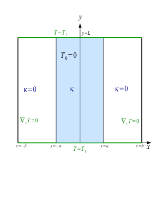
Figure 1: The Planar Sandwich. The inner material in blue (the meat) located within $-a\leq x\leq a$ is heat conducting with $\kappa>0$. The outer materials (the bread), located within $-b\leq x<-a$ and $a<x\leq b$, are not heat conducting and have $\kappa=0$. The boundary temperature is uniform in $x$ along the lower and upper boundaries, with temperatures $T(x,0)=T_{1}$ and $T(x,L)=T_{2}$. The temperature flux along the far left and right boundaries vanishes, $\partial_{x}T(\pm b,y)=0$. Finally, the initial temperature is taken to be $T_{0}(x,y)=0$ inside the entire region $(-b,b)\times(0,L)$.

The first test problem of Ref. Dawes2016 is a heat flow problem in 2D rectangular coordinates called the Planar Sandwich, illustrated in Fig. 1. The problem consists of three material layers aligned along the y-direction in a sandwich-like configuration. The outer two layers do not conduct heat ($\kappa=0$), while the inner layer is heat conducting with $\kappa>0$, forming a sandwich of conducting and non-conducting materials. The temperature boundary condition on the lower $y=0$ boundary is taken to be $T(x,y\!=\!0)=T_{1}$, while the temperature on the upper boundary is $T(x,y\!=\!L)=T_{2}$. The temperature flux in the $x$-direction on the far left and right ends of the sandwich vanishes, $\partial_{x}T(\pm b,y)=0$. Finally, the initial temperature inside the sandwich is taken to vanish, $T_{0}(x,y)=0$. Symmetry arguments reduce the problem to 1D heat flow in the $y$-direction, and in this subsection we shall orient the 1D rod of the previous section along the $y$-direction rather than the $x$-direction (in the remaining sections, however, we shall revert to the convention of heat flow along $x$). This brief change in convention allows us to keep with the original notation defined in Ref. Dawes2016 . The heat flow equation in the central region, $|x|\leq a$, reduces to 1D flow along the $y$-direction,

$$\frac{\partial T}{\partial t} = \kappa\,\frac{\partial^{2}T}{\partial y^{2}}\ .$$ (16)

We now represent the temperature profile as a function of $y$, so that $T=T(y,t)$, and the boundary conditions of the rod become $T(0,t)=T_{1}$ and $T(L,t)=T_{2}$, as in BC1. The initial condition becomes $T_{0}(y)=0$. The exact analytic solution was presented in Ref. Dawes2016 , and takes the form

$$T(y,t) = T_{1}+\frac{(T_{2}-T_{1})\,y}{L}+\sum_{n=1}^{\infty}B_{n}\,\sin(k_{n}y)\,e^{-\kappa\,k_{n}^{2}t}$$ (17)

$$k_{n} = \frac{n\pi}{L}\hskip 14.22636pt{\rm and}\hskip 14.22636ptB_{n}=\frac{2T_{2}(-1)^{n}-2T_{1}}{n\pi}\ ,$$ (18)

for $|x|\leq a$; and $T=0$ for $|x|>a$. Figure 2 illustrates a plot of the planar sandwich solution for the initial conditions $T_{1}=1$ and $T_{2}=0$, at several representative times $t=1\,,\,0.2\,,\,0.1\,,\,0.01,$ and $0.001$. The instance of the planar sandwich class used to plot the figure was created by the python call

solver = PlanarSandwich(T1=1, T2=0, L=2, Nsum=1000)  .

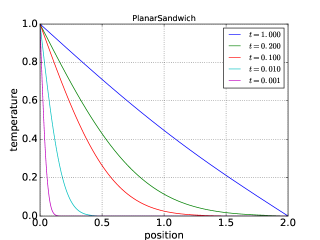
Figure 2: The Planar Sandwich in ExactPack: PlanarSandwich(T1=1, T2=0, L=2, Nsum=1000). The temperature profile is plotted at times $t=1,0.2,0.1,0.01$, and $0.001$. The BC’s are $T(0)=1$, T(L)=0, and The IC is $T_{0}=0$. The diffusion constant is $\kappa=1$, the length of the rod is $L=2$, and we have summed over 1000 terms in the series

This class instance sets the boundary conditions to $T_{1}=1$ and $T_{2}=0$, the length of the rod to $L=2$, and it sums over the first 1000 terms of the series. By default it also sets the IC to $T_{0}=0$. For each of the five representative values of $t$, we must create five solution objects, i.e.

t0 = 0.001
t1 = 0.01
...
soln0 = solver(y, t0)
soln1 = solver(y, t1)
...  ,

where y is an array of grid values ranging from $y=0$ to $y=L=2$. The solutions can then be plotted in the standard ExactPack manner, soln0.plot(), soln1.plot(), etc. The script that produces the plot in Fig. 2 is given in Appendix A.

In the following sections, we shall analyze heat flow in a 1D rod in some detail, and we will see that by modifying the boundary conditions, as well as the initial condition, we can form a number of variants of the planar sandwich. In our first variant, we take $T_{1}=0$ and $T_{2}=0$ (the homogeneous version of BC1), but we choose a nontrivial initial condition for $T_{0}(y)$. An arbitrary continuous function would suffice, but for simplicity we employ a linear initial condition for $T_{0}(y)$. Since, in this section, the heat flow is along the $y$-direction, the linear initial condition (15) must be translated into

$$T_{0}(y)=T_{0}^{\text{lin}}(y)=T_{\rm\scriptscriptstyle L}+\frac{T_{\rm\scriptscriptstyle R}-T_{\rm\scriptscriptstyle L}}{L}\,y\ .$$ (19)

As shown in the next section, the solution takes the form

$$T(y,t) = \sum_{n=1}^{\infty}B_{n}\,\sin(k_{n}y)\,e^{-\kappa\,k_{n}^{2}t}$$ (20)

$$k_{n} = \frac{n\pi}{L}\hskip 14.22636pt{\rm with}\hskip 14.22636ptB_{n}=\frac{2T_{\rm\scriptscriptstyle L}-T_{\rm\scriptscriptstyle R}(-1)^{n}}{n\pi}\ .$$ (21)

This is illustrated in Fig. 3 for the initial condition specified by $T_{\rm\scriptscriptstyle L}=3$ and $T_{\rm\scriptscriptstyle R}=4$. For this case, the class PlanarSandwich is instantiated by

solver = PlanarSandwich(T1=0, T2=0, TL=3, TR=4, L=2, Nsum=1000)  .

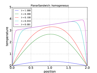
Figure 3: The Planar Sandwich: PlanarSandwich(T1=0, T2=0, TL=3, TR=4, L=2, Nsum=1000). Temperature profiles for the homogeneous planar sandwich at times $t=1,0.2,0.1,0.01$, and $0.001$, with $\kappa=1$, $L=2$, $T_{\rm\scriptscriptstyle L}=3$, $T_{\rm\scriptscriptstyle R}=4$ (and $T_{1}=T_{2}=0$). The boundary conditions $T_{1}=0$ and $T_{2}=0$ render the solution homogenous, while the initial condition $T_{0}(y)$, specified by $T_{\rm\scriptscriptstyle L}$ and $T_{\rm\scriptscriptstyle R}$, specifies the linear function (19) as the initial condition. As $t\to 0$, the solution $T(y,t)$ convergens nonuniformly on the open $y$-interval $(0,L)$ to $T_{0}(y)$.

The similarity between the coefficients $B_{n}$ in (21) and (18) is somewhat accidental, and arises from the choice of the linear initial condition (19), which, coincidentally, is the same form as the nonhomogeneous solution $\bar{T}(x)$ used to construct the original variant of the planar sandwich (18). It is this that accounts for the similarity. This example also illustrates how to override the default parameters in an ExactPack class, in this case, by setting $T_{1}=0$ and $T_{2}=0$. The default initial condition is $T_{0}(y)=0$, and this is why we did not need to specify the values of $T_{\rm\scriptscriptstyle L}$ and $T_{\rm\scriptscriptstyle R}$ in Fig. 2, and why we had to override these values in Fig. 3.

As another variant on the planar sandwich, we can choose vanishing heat flux on the upper and lower boundaries (as in BC2). This will be called the Hot Planar Sandwich, in analogy with the Hot Cylindrical Sandwich of Ref. Dawes2016 , and its solution takes the form

$$T(y,t) = \frac{A_{0}}{2}+\sum_{n=1}^{\infty}A_{n}\,\cos(k_{n}y)\,e^{-\kappa\,k_{n}^{2}t}$$ (22)

$$k_{n} = \frac{n\pi}{L}$$ (23)

$$A_{0} = \frac{T_{\rm\scriptscriptstyle L}+T_{\rm\scriptscriptstyle R}}{2}\hskip 14.22636pt{\rm and~{}for}~{}n\neq 0,\hskip 14.22636ptA_{n}=2\Big{(}T_{\rm\scriptscriptstyle L}-T_{\rm\scriptscriptstyle R}\Big{)}\frac{1-(-1)^{n}}{n^{2}\pi^{2}}\ .$$ (24)

This new variant of the planar sandwich can be instantiated by

solver = PlanarSandwichHot(F=0, TL=3, TR=3, L=2, Nsum=1000)  .

The heat flux $F$ on the boundaries has been set to zero, and a constant initial condition $T_{0}=3$ has been specified (by setting $T_{\rm\scriptscriptstyle L}=T_{\rm\scriptscriptstyle R}=3)$. The solution is illustrated in Fig. 4.

Figure 4: The Hot Planar Sandwich in ExactPack: PlanarSandwichHot(F=0, TL=3, TR=3, L=2, Nsum=1000). Since the heat flux on the boundaries vanishes, heat cannot escape from the material, and the temperature must remain constant in time. The temperature profile has been plotted for the times $t=1,0.2,0.1,0.01$, and $0.001$, and is indeed constant.

On physical grounds, heat cannot escape from the material, and the temperature must remain constant. In contrast, when the heat flux is nonzero, heat is free to flow from the sandwich to the environment, and the temperature need not remain constant. For a flux $F=1$, the change in the temperature profiles with time is illustrated in Fig. 5.

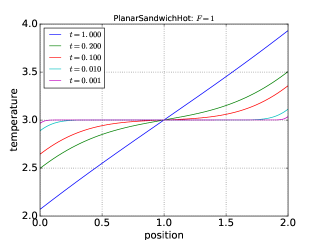
Figure 5: The Hot Planar Sandwich in ExactPack: PlanarSandwichHot(F=1, TL=3, TR=3, L=2, Nsum=1000). The profiles are plotted for times $t=1,0.2,0.1,0.01$, and $0.001$. The heat flux at the boundaries is $F=1$, and we see that the temperature profile changes as heat flows out of the rod.

Another variant on the planar sandwich is to choose vanishing heat flux on the upper boundary, $\partial_{y}T(L)=0$, and zero temperature on the lower boundary, $T(0)=0$. This is an example of boundary condition BC3, and the solution is called the Half Planar Sandwich. As we show in the next section, the solution takes the form

$$T(y,t) = \sum_{n=0}^{\infty}B_{n}\,\sin(k_{n}y)\,e^{-\kappa\,k_{n}^{2}t}$$ (25)

$$k_{n} = \frac{(2n+1)\pi}{L}\hskip 14.22636pt{\rm with}\hskip 14.22636ptB_{n}=\frac{4T_{\rm\scriptscriptstyle R}}{(2n+1)\pi}-\frac{8\big{(}T_{\rm\scriptscriptstyle R}-T_{\rm\scriptscriptstyle L}\big{)}}{(2n+1)^{2}\pi^{2}}\ .$$ (26)

Taking the initial condition $T_{0}=3$ ($T_{\rm\scriptscriptstyle L}=T_{\rm\scriptscriptstyle R}=3)$ gives Fig. 6, which is instantiated by solver = PlanarSandwichHalf(T=0, F=0, TL=3, TR=3, L=2, Nsum=1000)  .

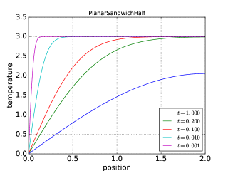
Figure 6: The Half Planar Sandwich in ExactPack: PlanarSandwichHalf(T=0, F=0, TL=3, TR=3, L=2, Nsum=1000). The profiles are plotted for times $t=1,0.2,0.1,0.01$, and $0.001$. Note that the profiles clearly satisfy the temperature on the left vanishes, and the derivative of the temperature on the right vanishes.

If we had chosen $\partial_{y}T(0)=0$ and $T(L)=0$, as in BC4, then the figure would have been reflected about the central point $y=1$, but otherwise physically identical.

II The Static Nonhomogeneous Problem

As previously discussed, the full nonhomogeneous problem is divided into two parts: (i) finding a general homogeneous solution $\tilde{T}(x,t)$, and (ii) finding a specific nonhomogeneous static solution $\bar{T}(x)$. Because of its simplicity, we first turn to solving the corresponding nonhomogeneous equations. We start with the static or equilibrium heat equation for $\bar{T}(x)$ with nonhomogeneous BC’s,

$${\rm DE}:\hskip 82.51282pt\frac{\partial^{2}\bar{T}(x)}{\partial x^{2}} = 0\hskip 85.35826pt0<x<L$$ (27)

$${\rm BC}:\hskip 33.0053pt\alpha_{1}\bar{T}(0)+\beta_{1}\bar{T}^{\prime}(0) = \gamma_{1}$$ (28)

$$\alpha_{2}\bar{T}(L)+\beta_{2}\bar{T}^{\prime}(L) = \gamma_{2}\ .$$ (29)

The solution to (27) is trivial, and may be written in the form,

$$\bar{T}(x)=a+b\,x\ ,$$ (30)

or alternatively,

$$\bar{T}(x) = T_{1}+\frac{T_{2}-T_{1}}{L}\,x\ .$$ (31)

The coefficients $a$ and $b$, or $T_{1}$ and $T_{2}$, are determined by the nonhomogeneous boundary conditions (28) and (29). Note that, coincidentally, that the static nonhomogeneous solution $\bar{T}(x)$ takes the same form as the linearized initial condition of (15), namely,

$$\bar{T}(x) = T_{0}^{\text{lin}}(x;T_{1},T_{2})\ .$$ (32)

While this is a fortuitous coincidence of 1D heat flow, and does not hold for 2D heat flow, (32) will be used in the following sections to simplify the algebra in calculating expansion coefficients for the homogenous and nonhomogeneous solutions. We turn now to finding the appropriate values of $T_{1}$ and $T_{2}$ for the case of general boundary conditions, and then for the four special cases,

1. (7)–(8)

2. (9)–(10)

3. (11)–(12)

4. (13)-(14)  .

II.1 General Boundary Conditions

As exhibited in (30)–(31), the nonhomogeneous solution $\bar{T}(x)$ can be expressed in the form

$$\bar{T}(x)=a+b\,x=T_{1}+\frac{T_{2}-T_{1}}{L}\,x\ ,$$ (33)

where $\bar{T}(0)=a=T_{1}$ and $\bar{T}(L)=a+bL=T_{2}$. The BC’s (28) and (29), and the solution (30), reduce to a linear equation in terms of $a$ and $b$,

$$\left(\begin{array}[]{cc}\alpha_{1}&\beta_{1}\\ \alpha_{2}&~{}\beta_{2}+\alpha_{2}L\end{array}\right)\left(\begin{array}[]{c}a\\ b\end{array}\right)=\left(\begin{array}[]{c}\gamma_{1}\\ \gamma_{2}\end{array}\right)\ .$$ (40)

Upon solving this equation we find

$$a = \frac{-\beta_{1}\gamma_{2}+\beta_{2}\gamma_{1}+L\alpha_{2}\gamma_{1}}{\alpha_{1}\beta_{2}-\alpha_{2}\beta_{1}+L\alpha_{1}\alpha_{2}}$$ (41)

$$b = \frac{\alpha_{1}\gamma_{2}-\alpha_{2}\gamma_{1}}{\alpha_{1}\beta_{2}-\alpha_{2}\beta_{1}+L\alpha_{1}\alpha_{2}}\ ,$$ (42)

or in terms of temperature parameters, $T_{1}=a$ and $T_{2}=a+bL$, we can write

$$T_{1} = \frac{\beta_{2}\gamma_{1}-\beta_{1}\gamma_{2}+L\alpha_{2}\gamma_{1}}{\alpha_{1}\beta_{2}-\alpha_{2}\beta_{1}+L\alpha_{1}\alpha_{2}}$$ (43)

$$T_{2} = \frac{\beta_{2}\gamma_{1}-\beta_{1}\gamma_{2}+L\alpha_{1}\gamma_{2}}{\alpha_{1}\beta_{2}-\alpha_{2}\beta_{1}+L\alpha_{1}\alpha_{2}}\ .$$ (44)

Note that the determinant of the linear equations vanishes for BC2, and we must handle this case separately.

II.2 Special Cases of the Static Problem

II.2.1 BC1

The first special boundary condition is (7) and (8),

$$\bar{T}(0) = T_{1}$$ (45)

$$\bar{T}(L) = T_{2}\ ,$$ (46)

with the solution taking the form (31),

$$\bar{T}(x) = T_{1}+\frac{T_{2}-T_{1}}{L}\,x\ .$$ (47)

The temperature coefficients $T_{1}$ and $T_{2}$ are given by the temperatures of the upper and lower boundaries in (45) and (46). Equivalently, the coefficients in (30) are just $a=T_{1}$ and $b=(T_{2}-T_{1})/L$.

II.2.2 BC2

Let us now find the nonhomogeneous equilibrium solution for the boundary conditions (9) and (10),

$$\partial_{x}\bar{T}(0) = F_{1}$$ (48)

$$\partial_{x}\bar{T}(L) = F_{2}\ ,$$ (49)

where $F_{1}$ and $F_{2}$ are the heat fluxes at $x=0$ and $x=L$, respectively, and are related to the boundary condition parameters in (28) and (29) by $F_{1}=\gamma_{1}/\beta_{1}$ and $F_{2}=\gamma_{2}/\beta_{2}$. As before, the general solution is $\bar{T}(x)=a+bx$, and we see that $\bar{T}^{\prime}(x)=b$ is independent of $x$. In other words, the heat flux at either end of the rod must be identical, $F_{1}=b=F_{2}$. In fact, this result follows from energy conservation, since, in equilibrium, the heat flowing into the rod must be equal the heat flowing out of the rod. Therefore, more correctly, we should have started with the boundary conditions

$$\partial_{x}\bar{T}(0) = F$$ (50)

$$\partial_{x}\bar{T}(L) = F\ ,$$ (51)

with

$$F=\frac{\gamma_{1}}{\beta_{1}}=\frac{\gamma_{2}}{\beta_{2}}\ .$$ (52)

As we saw in the previous section on general initial conditions, this case is singled out for special treatment. The value of the constant term $a$ is not uniquely determined in this case; however, we are free to set it to zero, giving

$$\bar{T}(x)=Fx\ .$$ (53)

There is nothing wrong with setting $a=0$, since we only need to find one nonhomogeneous solution, and (53) fits the bill. We can write this solution in the form (31), with

$$T_{1} = 0$$ (54)

$$T_{2} = FL\ .$$ (55)

II.2.3 BC3

The next set of boundary conditions are (11) and (12),

$$\bar{T}(0) = T_{1}$$ (56)

$$\partial_{x}\bar{T}(L) = F_{2}\ ,$$ (57)

and we can express the solution (31) in terms of the temperature $T_{1}$, and the effective temperature

$$T_{2} = T_{1}+F_{2}L=\frac{\gamma_{1}}{\alpha_{1}}+\frac{\gamma_{2}L}{\beta_{2}}\ .$$ (58)

II.2.4 BC4

The boundary conditions are (13) and (14),

$$\partial_{x}\bar{T}(0) = F_{1}$$ (59)

$$\bar{T}(L) = T_{2}\ ,$$ (60)

and the solution (31) can be written in terms of $T_{2}$ and the effective temperature

$$T_{1} = T_{2}-F_{1}L=\frac{\gamma_{2}}{\alpha_{2}}-\frac{\gamma_{1}L}{\beta_{1}}\ .$$ (61)

We have now found the static homogeneous solution in the form

$$\bar{T}(x)=T_{\scriptstyle 1}+\frac{(T_{1}-T_{1})\,x}{L}\ ,$$ (62)

where the temperatures in (62) are given by

1. $T_{1}$ and $T_{2}$

2. $T_{1}=0$ and $T_{2}=FL$

3. $T_{1}$ and $T_{2}=T_{1}+F_{2}l$

4. $T_{1}=T_{2}-F_{1}L$ and $T_{2}$  ,

and by (43) and (44) for general BC’s.

III The Homogeneous Problem

Now that we have found the appropriate nonhomogeneous solutions $\bar{T}(x)$, we turn to the more complicated task of finding the general homogeneous solutions $\tilde{T}(x,t)$. These solutions involve a Fourier sum over a discrete number of normal modes, the coefficients being determined by the initial conditions. These solutions depend upon The homogeneous equations of motion, for which $\gamma_{1}=0$ and $\gamma_{2}=0$ in the equations (1)–(4), take the form

$${\rm DE}:\hskip 106.12865pt\frac{\partial\tilde{T}(x,t)}{\partial t} = \kappa\,\frac{\partial^{2}\tilde{T}(x,t)}{\partial x^{2}}\hskip 34.14322pt0<x<L~{}{\rm and}~{}t>0$$ (63)

$${\rm BC}:\hskip 33.0053pt\alpha_{1}\tilde{T}(0,t)+\beta_{1}\partial_{x}\tilde{T}(0,t) = 0\hskip 83.93553ptt>0$$ (64)

$$\alpha_{2}\tilde{T}(L,t)+\beta_{2}\partial_{x}\tilde{T}(L,t) = 0$$

$${\rm IC}:\hskip 115.23373pt\tilde{T}(x,0) = T_{0}(x)\hskip 62.59596pt0<x<L\ .$$ (65)

As we have discussed in Section I.2, in all of our examples we shall employ the linear initial condition

$$T_{0}(x)=T_{0}^{\text{lin}}(x;T_{\rm\scriptscriptstyle L},T_{\rm\scriptscriptstyle R})=T_{\rm\scriptscriptstyle L}+\frac{T_{\rm\scriptscriptstyle R}-T_{\rm\scriptscriptstyle L}}{L}\,x\ .$$ (66)

The solution technique is by separation of variables, for which we assume the trial solution to be the product of independent functions of $x$ and $t$,

$$\tilde{T}(x,t)=X(x)\,U(t)\ .$$ (67)

Substituting this Ansatz into the heat equation gives

$$\frac{dU(t)}{dt}\,X(x)=\kappa\,U(t)\,\frac{d^{2}X(x)}{dx^{2}}\ ,$$ (68)

or

$$\frac{1}{\kappa}\,\frac{U^{\prime}(t)}{U(t)}=\frac{X^{\prime\prime}(x)}{X(x)}={\rm const}\equiv-k^{2}\ ,$$ (69)

where we have chosen the constant to have a negative value $-k^{2}$, and we have expressed derivatives of $U(t)$ and $X(x)$ by primes. As usual in the separation of variables technique, when two functions of different variables are equated, they must be equal to a constant, independent of the variables. The equation for $U(t)$ has the solution,

$$U_{k}(t) = U_{0}\,e^{-\kappa\,k^{2}t}\ ,$$ (70)

where we have introduced a $k$-subscript to indicate that the solution depends upon the value of $k$. The equations for $X$ reduce to

$$X^{\prime\prime}(x)+k^{2}X(x) = 0\hskip 51.21504pt0<x<L$$ (71)

$$\alpha_{1}X(0)+\beta_{1}X^{\prime}(0) = 0$$ (72)

$$\alpha_{2}X(L)+\beta_{2}X^{\prime}(L) = 0\ ,$$

where, now, the condition $X(x)=T_{0}(x)$ is the obvious statement that $X(x)$ is simply the initial condition of the original problem. The general solution to (71) is

$$X_{k}(x)=A_{k}\cos kx+B_{k}\sin kx\ ,$$ (73)

and when the BC’s are applied, the modes $X_{k}$ will be orthogonal,

$$\int_{0}^{L}dx\,X_{k}(x)X_{k^{\prime}}(x)=N_{k}\,\delta_{kk^{\prime}}\ .$$ (74)

Since the solutions are square integrable, and since the DE is liner and the BC’s are homogeneous, we have scaled $X_{k}$ to give an arbitrary normalization constant $N_{k}$, which can be chosen for convenience.

The general time dependent solution is a sum over all modes,

$$\tilde{T}(x,t)={\sum}_{k}D_{k}\,X_{k}(x)\,e^{-\kappa\,k^{2}t}\ ,$$ (75)

where we have absorbed the coefficient $U_{0}$ into the coefficients $D_{k}$. The $D_{k}$’s themselves are chosen so that the initial condition is satisfied,

$$\tilde{T}(x,0) = {\sum}_{k}D_{k}X_{k}(x)=T_{0}(x)$$ (76)

$$~{}~{}~{}\Rightarrow~{}~{}~{}D_{k} = \frac{1}{N_{k}}\int_{0}^{L}\!dx\,T_{0}(x)\,X_{k}(x)\ .$$ (77)

For tractability, we take the IC to be linear, as given in (15), where $T_{\rm\scriptscriptstyle L}$ is the temperature at $x=0^{+}$, and $T_{\rm\scriptscriptstyle R}$ is the temperature at $x=L^{-}$. When $T_{\rm\scriptscriptstyle L}=T_{\rm\scriptscriptstyle R}$, the IC is a constant. The linear initial condition (15) contains two temperature parameters, $T_{0}(x)=T_{0}^{\text{lin}}(x;T_{\rm\scriptscriptstyle L},T_{\rm\scriptscriptstyle R})$, and therefore the corresponding Fourier coefficients are functions of these parameters,

$$D_{k}^{\text{lin}}(T_{\rm\scriptscriptstyle L},T_{\rm\scriptscriptstyle R}) = \frac{1}{N_{k}}\int_{0}^{L}\!dx\,T_{0}^{\text{lin}}(x;T_{\rm\scriptscriptstyle L},T_{\rm\scriptscriptstyle R})\,X_{k}(x)\ .$$ (78)

When solving for the full nonhomogeneous solution (NH), rather than using (77) to find $D_{k}$, we need to choose the coefficients such that

$$D_{k}^{\rm\scriptscriptstyle NH} = \frac{1}{N_{k}}\int_{0}^{L}\!dx\,\Big{[}T_{0}(x)-\bar{T}(x)\Big{]}\,X_{k}(x)$$ (79)

$$= \frac{1}{N_{k}}\int_{0}^{L}\!dx\,\Big{[}T_{0}^{\text{lin}}(x;T_{\rm\scriptscriptstyle L},T_{\rm\scriptscriptstyle R})-T_{0}^{\text{lin}}(x;T_{1},T_{2})\Big{]}\,X_{k}(x)\ ,$$ (80)

where we have written the nonhomogeneous solution $\bar{T}(x)$ can be written

$$\bar{T}(x)=T_{0}^{\text{lin}}(x;T_{1},T_{2})\ ,$$ (81)

as discussed in Section II. Therefore, the nonhomogeneous coefficients can be expressed in terms of the homogeneous coefficients by

$$D_{k}^{\rm\scriptscriptstyle NH}(T_{\rm\scriptscriptstyle L},T_{\rm\scriptscriptstyle R},T_{1},T_{2}) = D_{k}^{\text{lin}}(T_{\rm\scriptscriptstyle L}-T_{1},T_{\rm\scriptscriptstyle R}-T_{2})$$ (82)

$$= \frac{1}{N_{k}}\int_{0}^{L}\!dx\,T_{0}^{\text{lin}}(x,T_{\rm\scriptscriptstyle L}-T_{1},T_{\rm\scriptscriptstyle R}-T_{2})\,X_{k}(x)\ .$$ (83)

We will employ this equation in the final section.

It is instructive to prove the orthogonality relation (74) directly from the differential equation. To see this, multiply (71) by $X_{k^{\prime}}$, and then write the result in the two alternate forms,

$$X_{k^{\prime}}\Big{[}X_{k}^{\prime\prime}+k^{2}X_{k}\Big{]} = 0$$ (84)

$$X_{k}\Big{[}X_{k^{\prime}}^{\prime\prime}+k^{\prime\,2}X_{k^{\prime}}\Big{]} = 0\ .$$ (85)

Upon subtracting these equations, and then integrating over space, we find

$$(k^{2}-k^{\prime\,2})\int_{0}^{L}\!dx\,X_{k}\,X_{k^{\prime}} = \int_{0}^{L}\!dx\,\Big{[}X_{k}X_{k^{\prime}}^{\prime\prime}-X_{k^{\prime}}X_{k}^{\prime\prime}\Big{]}$$

$$= \int_{0}^{L}\!dx\,\Big{[}\frac{d}{dx}\,\Big{(}X_{k}X_{k^{\prime}}^{\prime}\Big{)}-X_{k}^{\prime}X_{k^{\prime}}^{\prime}-\frac{d}{dx}\Big{(}X_{k^{\prime}}X_{k}^{\prime}\Big{)}+X_{k^{\prime}}^{\prime}X_{k}^{\prime}\Big{]}$$

$$= \int_{0}^{L}\!dx\,\frac{d}{dx}\,\Big{(}X_{k}X_{k^{\prime}}^{\prime}-X_{k^{\prime}}X_{k}^{\prime}\Big{)}$$ (87)

$$= \Big{(}X_{k}X_{k^{\prime}}^{\prime}-X_{k^{\prime}}X_{k}^{\prime}\Big{)}\Big{|}_{0}^{L}=0\ ,$$ (88)

where each contribution from $x=0$ and $x=L$ vanishes separately because of their respective boundary conditions. We therefore arrive at

$$(k^{2}-k^{\prime\,2})\int_{0}^{L}\!dx\,X_{k}\,X_{k^{\prime}}=0\ .$$ (89)

Provided $k\neq k^{\prime}$, we can divide (89) by $k^{2}-k^{\prime\,2}$ to obtain

$$\int_{0}^{L}\!dx\,X_{k}(x)\,X_{k^{\prime}}(x) = 0~{}~{}~{}{\rm when}~{}k\neq k^{\prime}\ .$$ (90)

However, when $k=k^{\prime}$, (89) gives no constraint on the corresponding normalization integral; however, since the BC’s are homogeneous, we are free to normalize $X_{k}$ over $[0,L]$ such that $\int dx\,X_{k}^{2}=N_{k}$, for any convenient choice of $N_{k}$.

III.1 Special Cases of the Homogeneous Problem

We now find the homogeneous solutions for four special boundary conditions, BC1–BC4.

III.1.1 BC1

The first case holds the temperature fixed to zero at both ends of the rod,

$$\tilde{T}(0,t) = 0$$ (91)

$$\tilde{T}(L,t) = 0\ .$$ (92)

The general solution $X_{k}(x)\!=\!A_{k}\cos kx+B_{k}\sin kx$ reduces to $X_{k}(x)=B_{k}\sin kx$ under (91), while (92) restricts the wave numbers to satisfy $\sin kL=0$, i.e. $k=k_{n}=n\pi/L$ for $n=1,2,3,\cdots$. Note that $n=0$ does not contribute, since this gives the trivial vanishing solution. It is convenient to express the modes by $X_{n}(x)=\sin k_{n}x$, separating the coefficient $B_{n}=B_{k_{n}}$ from the mode $X_{n}$ itself. The homogeneous solution then takes the form

$$\tilde{T}(x,t) = \sum_{n=1}^{\infty}B_{n}\,X_{n}(x)\,e^{-\kappa\,k_{n}^{2}t}$$ (93)

$$X_{n}(x) = \sin k_{n}x$$ (94)

$$k_{n} = \frac{n\pi}{L}\hskip 28.45274ptn=1,2,3,\cdots\ .$$ (95)

The tilde over the temperature is meant to explicitly remind us that this is the general homogeneous solution. The orthogonality condition on the modes $X_{n}$ can be checked by a simple integration,

$$\int_{0}^{L}dx\,X_{n}(x)X_{m}(x) = \frac{L}{2}\,\delta_{nm}\ .$$ (96)

For an initial condition $\tilde{T}(x,0)=T_{0}(x)$, we can calculate the corresponding coefficients in the Fourier sum,

$$B_{n}=\frac{2}{L}\int_{0}^{L}dx\,T_{0}(x)\sin k_{n}x\ .$$ (97)

For the linear initial condition (15), a simple calculation gives

$$B_{n} = 2T_{\rm\scriptscriptstyle L}\,\frac{1-(-1)^{n}}{n\pi}+2(T_{\rm\scriptscriptstyle L}-T_{\rm\scriptscriptstyle R})\,\frac{(-1)^{n}}{n\pi}$$ (98)

$$= \frac{2T_{\rm\scriptscriptstyle L}-2T_{\rm\scriptscriptstyle R}(-1)^{n}}{n\pi}\ .$$ (99)

The first two terms in line (98) are the constant and linear contributions of $T_{0}(x)$, respectively, and a typical solution is illustrated in Fig. 7. The ExactPack object used to create Fig. 7 is the class Rod1D, which takes the following boundary and initial condition arguments

Rod1D(alpha1=1, beta1=0, alpha2=1, beta2=0, TL=3, TR=4)  .

This Figure is identical to Fig. 3, and is meant to illustrate the parent class Rod1D from which PlanarSandwich inherits.

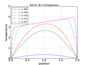
Figure 7: This is the same as Fig. 3, the homogeneous planar sandwich, except we use the base class Rod1D(alpha1=1, beta1=0, alpha2=1, beta2=0, TL=3, TR=4).

III.1.2 BC2

The second special boundary condition that we consider sets the heat flux at both ends of the rod to zero,

$$\partial_{x}\tilde{T}(0,t) = 0$$ (100)

$$\partial_{x}\tilde{T}(L,t) = 0\ .$$ (101)

This is the hot planar sandwich of the introduction. The general solution $X_{k}(x)\!=\!A_{k}\cos kx+B_{k}\sin kx$ reduces to $X_{k}(x)=A_{k}\cos kx$ under (100) , while (101) restricts the wave numbers to $k\sin kL=0$, so that $k=k_{n}=n\pi/L$ for $n=0,1,2\cdots$. In this case, the $n=0$ mode is permitted (and essential). As before we separate the Fourier coefficients $A_{n}=A_{k_{n}}$ from the mode functions themselves, $X_{n}=X_{k_{n}}$, and we write

$$\tilde{T}(x,t) = \frac{A_{0}}{2}+\sum_{n=1}^{\infty}A_{n}\,X_{n}(x)\,e^{-\kappa\,k_{n}^{2}t}$$ (102)

$$X_{n}(x) = \cos k_{n}x$$ (103)

$$k_{n} = \frac{n\pi}{L}\hskip 28.45274ptn=0,1,2,\cdots\ .$$ (104)

A conventional factor of $1/2$ has been used in the $n=0$ term because of the difference in normalization between $n=0$ and $n\neq 0$,

$$\int_{0}^{L}dx\,X_{0}^{2}(x) = L$$ (105)

$$\int_{0}^{L}dx\,X_{n}^{2}(x) = \frac{L}{2}~{}~{}~{}~{}n\neq 0\ ,$$ (106)

since $X_{0}(x)=1$ and $X_{n}=\cos k_{n}x$. Given the initial condition $\tilde{T}(x,0)=T_{0}(x)$, the Fourier modes become

$$A_{n}=\frac{2}{L}\,\int_{0}^{L}dx\,T_{0}(x)\cos k_{n}x\ .$$ (107)

This holds for all values of $n$, including $n=0$, because we have inserted the factor of 1/2 in the $A_{0}$-term of (102). For simplicity, we will take the linear initial condition (15) for $T_{0}(x)$, in which case, (107) gives the coefficients

$$\frac{A_{0}}{2} = \frac{1}{2}\Big{(}T_{\rm\scriptscriptstyle L}+T_{\rm\scriptscriptstyle R}\Big{)}$$ (108)

$$A_{n} = 2\,\Big{(}T_{\rm\scriptscriptstyle L}-T_{\rm\scriptscriptstyle R}\Big{)}\,\frac{1-(-1)^{n}}{n^{2}\pi^{2}}\ .$$ (109)

For pedagogical purposes, let us be pedantic and work through the algebra for the $A_{n}$ coefficients, doing the $n=0$ case first:

$$\frac{A_{0}}{2} = \frac{1}{L}\int_{0}^{L}\,T_{0}(x)=\frac{1}{L}\int_{0}^{L}\,\left[T_{\rm\scriptscriptstyle L}+\frac{T_{\rm\scriptscriptstyle R}-T_{\rm\scriptscriptstyle L}}{L}\,x\right]$$ (110)

$$= T_{\scriptstyle L}+\left[\frac{T_{\rm\scriptscriptstyle R}-T_{\rm\scriptscriptstyle L}}{2}\right]=\frac{1}{2}\left[T_{\rm\scriptscriptstyle R}+T_{\rm\scriptscriptstyle L}\right]\ .$$ (111)

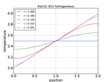
Figure 8: BC2 with $\kappa=1$, $L=2$, $T_{\rm\scriptscriptstyle L}=3$, $T_{\rm\scriptscriptstyle R}=4$. Rod1D(alpha1=0, beta1=1, alpha2=0, beta2=1, TL=3, TR=4).

Next, taking $n\neq 0$, we find:

$$A_{n} = \frac{2}{L}\int_{0}^{L}dx\,T_{0}(x)\cos k_{n}x$$ (112)

$$= \frac{2}{L}\int_{0}^{L}dx\,\left[T_{\rm\scriptscriptstyle L}+\frac{T_{\rm\scriptscriptstyle R}-T_{\rm\scriptscriptstyle L}}{L}\,x\right]\cos k_{n}x$$ (113)

$$= T_{\rm\scriptscriptstyle L}\,\frac{2}{L}\int_{0}^{L}dx\,\cos k_{n}x+\Big{(}T_{\rm\scriptscriptstyle R}-T_{\rm\scriptscriptstyle L}\Big{)}\frac{2}{L^{2}}\int_{0}^{L}dx\,x\,\cos k_{n}x\ .$$ (114)

The first term integrates to zero since

$$\frac{2}{L}\int_{0}^{L}dx\,\cos k_{n}x = \frac{2}{L}\,\sin k_{n}x\Big{|}_{x=0}^{x=L}=0\ ,$$ (115)

and the second term gives

$$\frac{2}{L^{2}}\int_{0}^{L}dx\,x\,\cos k_{n}x = \frac{2}{L^{2}}\left[\frac{\cos k_{n}x}{k_{n}^{2}}+\frac{x\sin k_{n}x}{k_{n}}\right]_{x=0}^{x=L}$$ (116)

$$= \frac{2}{L^{2}}\,\frac{L^{2}}{n^{2}\pi^{2}}\,\Big{[}\cos k_{n}L-1\Big{]}=2\,\frac{(-1)^{n}-1}{n^{2}\pi^{2}}\ ,$$ (117)

which leads to (109).

III.1.3 BC3

The next specialized boundary condition is

$$\tilde{T}(0,t) = 0$$ (118)

$$\partial_{x}\tilde{T}(L,t) = 0\ .$$ (119)

The general solution $X_{k}(x)\!=\!A_{k}\cos kx+B_{k}\sin kx$ under (118) reduces to $X_{k}(x)=B_{k}\sin kx$, while (119) restricts the wave numbers to $k\cos kL=0$, so that $k=k_{n}=(2n+1)\pi/2L$ for $n=0,1,2\cdots$. The general homogeneous solution is therefore

$$\tilde{T}(x,t) = \sum_{n=0}^{\infty}B_{n}\,X_{n}(x)\,e^{-\kappa\,k_{n}^{2}t}$$ (120)

$$X_{n}(x) = \sin k_{n}x$$ (121)

$$k_{n} = \frac{(2n+1)\pi}{2L}\hskip 28.45274ptn=0,1,2,\cdots\ .$$ (122)

The initial condition $\tilde{T}(x,0)=T_{0}(x)$ gives the Fourier modes

$$B_{n}=\frac{2}{L}\,\int_{0}^{L}dx\,T_{0}(x)\sin k_{n}x\ ,$$ (123)

and, as before, upon taking the linear function (15), we find

$$B_{n} = \frac{4T_{\rm\scriptscriptstyle L}}{(2n+1)\pi}+4\big{(}T_{\rm\scriptscriptstyle R}-T_{\rm\scriptscriptstyle L}\big{)}\left[\frac{1}{(2n+1)\pi}-\frac{2}{(2n+1)^{2}\pi^{2}}\right]$$ (124)

$$= \frac{4T_{\rm\scriptscriptstyle R}}{(2n+1)\pi}-\frac{8\big{(}T_{\rm\scriptscriptstyle R}-T_{\rm\scriptscriptstyle L}\big{)}}{(2n+1)^{2}\pi^{2}}\ .$$ (125)

Before plotting this example, let us examine the next boundary condition.

III.1.4 BC4

The last special case is the boundary condition

$$\partial_{x}\tilde{T}(0,t) = 0$$ (126)

$$\tilde{T}(L,t) = 0\ .$$ (127)

The general solution $X_{k}(x)\!=\!A_{k}\cos kx+B_{k}\sin kx$ reduces to $X_{k}(x)=A_{k}\cos kx$ under (118), while (127) restricts the wave numbers to $\cos kL=0$, i.e. $k=k_{n}=(2n+1)\pi/2L$ for $n=0,1,2\cdots$, which gives rise to the homogeneous solution

$$\tilde{T}(x,t) = \sum_{n=0}^{\infty}A_{n}\,X_{n}(x)\,e^{-\kappa\,k_{n}^{2}t}$$ (128)

$$X_{n}(x) = \cos k_{n}x$$ (129)

$$k_{n} = \frac{(2n+1)\pi}{2L}\hskip 28.45274ptn=0,1,2,\cdots\ .$$ (130)

Similar to (123), the mode coefficient is

$$A_{n}=\frac{2}{L}\,\int_{0}^{L}dx\,T_{0}(x)\cos k_{n}x\ ,$$ (131)

and, upon taking the linear initial condition (15), we find

$$A_{n} = 4T_{\rm\scriptscriptstyle L}\,\frac{(-1)^{n}}{(2n+1)\pi}-8\Big{(}T_{\rm\scriptscriptstyle R}-T_{\rm\scriptscriptstyle L}\Big{)}\,\frac{1-(-1)^{n}}{(2n+1)^{2}\,\pi^{2}}\ .$$ (132)

The cases BC3 and BC4 are plotted in Fig. 9.

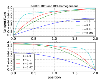
Figure 9: BC3 and BC4 for $\kappa=1$, $L=2$, $T_{\rm\scriptscriptstyle L}=T_{\rm\scriptscriptstyle R}=3$. By symmetry principles, the two profiles are mirror images of one another. BC3 is instantiated by Rod1D(alpha1=1, beta1=0, alpha2=0, beta2=1, TL=3, TR=4), and BC4 by Rod1D(alpha1=0, beta1=1, alpha2=1, beta2=0, TL=4, TR=3). Note that $T_{\rm\scriptscriptstyle L}$ and $T_{\rm\scriptscriptstyle R}$ are interchanged between BC3 and BC4.

III.2 General Boundary Conditions

We now turn to the general form of the boundary conditions, which, expressed in terms of $X$, take the form

$$\alpha_{1}X_{k}(0)+\beta_{1}X_{k}^{\prime}(0) = 0$$ (133)

$$\alpha_{2}X_{k}(L)+\beta_{2}X_{k}^{\prime}(L) = 0\ .$$ (134)

The solution and its derivative are

$$X_{k}(x) = A\cos kx+B\sin kx$$ (135)

$$X_{k}^{\prime}(x) = -Ak\sin kx+Bk\cos kx\ .$$ (136)

Substituting this into (133) and (134) gives

$$\alpha_{1}A+\beta_{1}Bk = 0$$ (137)

$$\alpha_{2}\Big{[}A\cos kL+B\sin kL\Big{]}+\beta_{2}\Big{[}-Ak\sin kL+Bk\cos kL\Big{]} = 0\ .$$ (138)

Upon diving by $\cos kL\neq 0$, can write (138) as

$$(\alpha_{2}\,B-\beta_{2}\,Ak)\tan kL+\alpha_{2}A+\beta_{2}\,Bk = 0\ ,$$ (139)

or

$$\tan kL = \frac{\beta_{2}\,Bk+\alpha_{2}A}{\beta_{2}\,Ak-\alpha_{2}\,B}\ .$$ (140)

From (137) we have $Bk=-\alpha_{1}A/\beta_{1}$ (if $\beta_{1}\neq 0)$, and substituting into (140) gives

$$\tan kL = \frac{-(\alpha_{1}\beta_{2}/\beta_{1})+\alpha_{2}}{\beta_{2}\,k+\alpha_{2}\,(\alpha_{1}/\beta_{1}k)}\cdot\frac{\beta_{1}k}{\beta_{1}k}$$ (141)

$$= \frac{-\alpha_{1}\beta_{2}\,k+\alpha_{2}\beta_{1}k}{\beta_{1}\beta_{2}\,k^{2}+\alpha_{2}\,\alpha_{1}}\ .$$ (142)

Setting $\mu\equiv kL$ and $\bar{\beta}_{i}\equiv\beta_{i}/L$, we can write (142) in the form

$$\tan\mu = \frac{(\alpha_{2}\bar{\beta}_{1}-\alpha_{1}\bar{\beta}_{2})\,\mu}{\alpha_{1}\alpha_{2}+\bar{\beta}_{1}\bar{\beta}_{2}\,\mu^{2}}\ .$$ (143)

The solution is illustrated in Fig. 10.

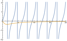
Figure 10: The roots $\mu_{n}$ for $\alpha_{1}=1$, $\bar{\beta}=1/2$, $\alpha_{2}=1$, and $\bar{\beta}_{2}=1$. For $L=2$ this gives $\beta_{1}=1$ and $\beta_{2}=2$.

Equation (143) will give solutions $\mu_{n}$ for $n=0,1,2,\cdots$ and with wave numbers

$$k_{n}=\frac{\mu_{n}}{L}\ .$$ (144)

Note that $\mu_{0}=0$, and therefore $k_{0}=0$. The solution now takes the form

$$X_{n}(x) = A_{n}\cos k_{n}x+B_{n}\sin k_{n}$$ (145)

$$A_{n} = -\frac{\beta_{1}k_{n}}{\alpha_{1}}\,B_{n}\ ,$$ (146)

where $\alpha_{1}\neq 0$. The case of $\alpha_{1}=0$ will be handled separately. Setting $B_{n}=1$ for convenient, the solution (145) can be expressed as

$$X_{n}(x) = \sin k_{n}x-\frac{\beta_{1}k_{n}}{\alpha_{1}}\cos k_{n}x\ .$$ (147)

And the general solution is

$$X(x) = \sum_{n=1}^{\infty}B_{n}X_{n}(x)\ ,$$ (148)

as the $n=0$ term does not contribute. Note that

$$\int_{0}^{L}dx\,X_{n}(x)X_{m}(x)=0~{}~{}~{}{\rm for}~{}n\neq m$$ (149)

and

$$\int_{0}^{L}dx\,X_{n}^{2}(x) = \frac{1}{4k_{n}\alpha_{1}^{2}}\Bigg{[}-2\alpha_{1}\beta_{1}k_{n}+2(\beta_{1}^{2}k_{n}^{2}+\alpha_{1}^{2})k_{n}L+$$

$$\hskip 42.67912pt2\alpha_{1}\beta_{1}k_{n}\cos 2k_{n}L+(\beta_{1}^{2}k_{n}^{2}-\alpha_{1}^{2})\sin 2k_{n}L\Bigg{]}\ .$$

In summary,

$$\int_{0}^{L}dx\,X_{n}(x)X_{m}(x)=N_{n}\,\delta_{nm}\ ,$$ (151)

$$N_{n}=\frac{1}{4k_{n}\alpha_{1}^{2}}\Big{[}-2\alpha_{1}\beta_{1}k_{n}+2(\beta_{1}^{2}k_{n}^{2}+\alpha_{1}^{2})k_{n}L+2\alpha_{1}\beta_{1}k_{n}\cos 2k_{n}L+(\beta_{1}^{2}k_{n}^{2}-\alpha_{1}^{2})\sin 2k_{n}L\Big{]}\ .$$

(152)

Since $k_{0}=0$, we have $X_{0}(x)=0$, so we are free to restrict $n=1,2,3,\cdots$, and the general solution is

$$X(x) = \sum_{n=1}^{\infty}D_{n}\,X_{n}(x)\ .$$ (153)

Since $X(x)=T_{0}(x)$, we find

$$D_{n}=\frac{1}{N_{n}}\int_{0}^{L}dx\,T_{0}(x)X_{n}(x)\ .$$ (154)

It is convenient for numerical work to express this in terms of $A_{n}$ and $B_{n}$ coefficients:

$$X(x) = \sum_{n=1}^{\infty}D_{n}\,\Big{[}-\frac{\beta_{1}k_{n}}{\alpha_{1}}\,\cos k_{n}x+\sin k_{n}x\Big{]}$$ (155)

$$= \sum_{n=1}^{\infty}\Big{[}A_{n}\cos k_{n}x+B_{n}\sin k_{n}x\Big{]}{\rm~{}~{}~{}with}$$ (156)

$$A_{n} = -\frac{\beta_{1}k_{n}}{\alpha_{1}}\,D_{n}$$

$$B_{n} = D_{n}\ .$$

The temperature $\tilde{T}(x,t)$ is therefore,

$$\tilde{T}(x,t) = \sum_{n=1}^{\infty}\Big{[}A_{n}\cos k_{n}x+B_{n}\sin k_{n}x\Big{]}\,e^{-\kappa\,k_{n}^{2}t}$$ (157)

$$B_{n} = \frac{1}{N_{n}}\int_{0}^{L}dx\,T_{0}(x)X_{n}(x)$$ (158)

$$A_{n} = -\frac{\beta_{1}k_{n}}{\alpha_{1}}\,B_{n}\ .$$ (159)

For $T_{0}^{a}(x)=T_{1}$ we have

$$B_{n}^{a} = \frac{T_{1}}{N_{n}}\,\left[\frac{1-\cos k_{n}L}{k_{n}}-\frac{\beta_{1}\sin k_{n}L}{\alpha_{1}}\right]\ .$$ (160)

For $T_{0}^{b}(x)=(T_{2}-T_{1})\,x/L$ we have

$$B_{n}^{b} = \frac{T_{2}-T_{1}}{N_{n}\,L}\,\frac{1}{\alpha_{1}k_{n}^{2}}\,\Big{[}\beta_{1}k_{n}-(\alpha_{1}k_{n}L+\beta_{1}k_{n})\cos k_{n}L+(\alpha_{1}-\beta_{1}k_{n}^{2}L)\sin k_{n}L\Big{]}\ ,$$ (161)

with $B_{n}=B_{n}^{a}+B_{n}^{b}$.

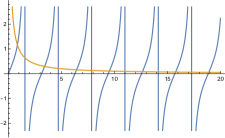
Figure 11: The roots $\mu_{n}$ for $\alpha_{1}=0$, $\alpha_{2}=1$, and $\bar{\beta}_{2}=1$. For $L=2$ we have $\beta_{2}=2$.

Let us now consider the case of $\alpha_{1}=0$, so that (143) becomes

$$\tan\mu = \frac{a}{\mu}~{}~{}~{}~{}{\rm with}~{}~{}a=\alpha_{2}/\bar{\beta}_{2}\ .$$ (162)

We can find an approximate solution for large values of $\mu$: since the RHS is very small for $\mu\gg 1$, we must solve $\tan\mu=0$, and therefore $\mu_{n}^{(0)}=n\pi$. The exact solution can be expressed as $\mu_{n}=n\pi+h$, where $h$ is small and unknown. Then ${\rm LHS}=\tan(n\pi+h)=\tan(h)=h+{\cal O}(h^{2})$. Similarly, ${\rm RHS}=a/(n\pi+h)=(a/n\pi)\big{(}1+h/n\pi\big{)}^{-1}=(a/n\pi)\big{(}1-h/n\pi\big{)}+{\cal O}([h/n]^{2})=a/n\pi-ah+{\cal O}([h/n]^{2})$, thus

$$h=\frac{a}{n\pi}-ah~{}~{}~{}\Rightarrow~{}~{}~{}h=\frac{a}{1+a}\,\frac{1}{n\pi}\ ,$$ (163)

and the first order solution becomes

$$\mu_{n}^{(1)}=n\pi+\frac{a}{1+a}\,\frac{1}{n\pi}+{\cal O}(1/n^{2})\ .$$ (164)

This can be used as an initial guess when using an iteration method to find the $\mu_{n}$. The solution is

$$T(x,t) = \sum_{n=1}^{\infty}A_{n}X_{n}(x)\,e^{-\kappa\,k_{n}^{2}t}$$ (165)

$$X_{n}(x) = \cos k_{n}L$$ (166)

$$\int_{0}^{L}dx\,X_{n}(x)X_{m}(x) = N_{n}\,\delta_{nm}$$ (167)

$$N_{n} = \frac{1}{4k_{n}}\,\Big{[}2k_{n}L+\sin 2k_{n}L\Big{]}\ ,$$ (168)

and

$$A_{n} = \frac{1}{N_{n}}\int_{0}^{L}dx\,T(x,0)X_{n}(x)$$ (169)

$$= \frac{T_{1}}{k_{n}}\,\sin k_{n}L+\frac{T_{2}-T_{1}}{k_{n}^{2}L}\,\Big{[}-1+\cos k_{n}L+k_{n}L\sin k_{n}L\Big{]}\ .$$ (170)

IV The Full Nonhomogeneous Problem

Suppose now that $\tilde{T}(x,t)$ is a general solution to the homogeneous problem as described in the previous section. Also suppose that $\bar{T}(x)$ is a specific solution to the nonhomogeneous problem as described in the previous section, then

$$T(x,t) = \tilde{T}(x,t)+\bar{T}(x)$$ (171)

is the solution to the nonhomogeneous problem (1)–(4). The general homogeneous solution, and the specific nonhomogeneous solution take the form

$$\tilde{T}(x,t) = \sum_{n}D_{n}\,X_{n}(x)\,e^{-\kappa\,k_{n}^{2}t}$$ (172)

$$\bar{T}(x) = T_{0}^{\text{lin}}(x;T_{1},T_{2})=T_{1}+\frac{T_{2}-T_{1}}{L}\,x\ ,$$ (173)

where the coefficients are chosen to satisfy the initial condition,

$$D_{n} = \int_{0}^{L}\Big{[}T_{0}(x)-\bar{T}(x)\Big{]}X_{n}(x)\ ,$$ (174)

with $\bar{T}(x)$ given by (173), and $T_{0}(x)$ given by

$$T_{0}(x) = T_{0}^{\text{lin}}(x;T_{\rm\scriptscriptstyle L},T_{\rm\scriptscriptstyle R})=T_{\rm\scriptscriptstyle L}+\frac{T_{\rm\scriptscriptstyle R}-T_{\rm\scriptscriptstyle L}}{L}\,x\ .$$ (175)

Since $T_{0}(x)$ and $\bar{T}(x)$ are of the same functional form, we can write

$$T_{0}(x)-\bar{T}(x) \equiv T_{0}^{\text{lin}}(x;T_{a},T_{b})=T_{a}+\frac{T_{b}-T_{a}}{L}\,x$$ (176)

$$T_{a} = T_{\rm\scriptscriptstyle L}-T_{1}$$ (177)

$$T_{b} = T_{\rm\scriptscriptstyle R}-T_{2}\ ,$$ (178)

where we have expressed the parametric dependence upon temperature explicitly in $T_{0}^{\text{lin}}$. Therefore,

$$D_{n} = D_{n}^{\text{lin}}(T_{\rm\scriptscriptstyle L}-T_{1},T_{\rm\scriptscriptstyle R}-T_{2})\equiv\int_{0}^{L}T_{0}^{\text{lin}}(x;T_{\rm\scriptscriptstyle L}-T_{1},T_{\rm\scriptscriptstyle R}-T_{2})\,X_{n}(x)\ .$$ (179)

This is why the the planar sandwich and the homogeneous planar sandwich have such similar coefficients,

$$B_{n}^{\text{planar sand}} = \phantom{-}D_{n}^{\text{lin}}(T_{1},T_{2})$$ (180)

$$B_{n}^{\text{hom planar sand}} = -D_{n}^{\text{lin}}(T_{\rm\scriptscriptstyle L},T_{\rm\scriptscriptstyle R})\ .$$ (181)

IV.1 Special Cases of the Nonhomogeneous Problem

We turn now to the full set of nonhomogeneous problems for the special cases considered in the previous section.

IV.1.1 BC1

The complete solution for the nonhomogeneous BC’s

$$T(0,t) = T_{1}$$ (182)

$$T(L,t) = T_{2}$$ (183)

is

$$T(x,t)=T_{1}+\frac{(T_{2}-T_{1})x}{L}+\sum_{n=1}^{\infty}B_{n}\,\sin k_{n}x\,e^{-\kappa\,k_{n}^{2}t}\ .$$ (184)

Recall that these BC’s corresponds to $\beta_{1}=\beta_{2}=0$ with and $\gamma_{1}/\alpha_{1}=T_{1}$ and $\gamma_{2}/\alpha_{2}=T_{2}$ in Eqs. (7) and (8 ). In terms of the BC’s, we can write this as

$$\bar{T}(x)=T_{1}+\frac{T_{2}-T_{1}}{L}\,x\ .$$ (185)

The nonhomogeneous coefficients are found by

$$B_{n} = \int_{0}^{L}\Big{[}T_{0}(x)-\bar{T}(x)\Big{]}\sin k_{n}x\ .$$ (186)

Since we have taken the $T_{0}(x)$ to be a linear equation, as is $\bar{T}(x)$, we can use the previous results for a linear initial conditions by substituting $T_{\rm\scriptscriptstyle L}\to T_{a}=T_{\rm\scriptscriptstyle L}-T_{1}$ and $T_{\rm\scriptscriptstyle R}\to T_{b}=T_{\rm\scriptscriptstyle R}-T_{2}$ into (99), as explained in the previous section. In other words,

$$T_{0}(x)-\bar{T}(x) = T_{a}+\frac{T_{b}-T_{a}}{L}$$ (187)

$$T_{a} = T_{\rm\scriptscriptstyle L}-T_{1}$$ (188)

$$T_{b} = T_{\rm\scriptscriptstyle R}-T_{2}\ ,$$ (189)

and the coefficients of the nonhomogeneous solution become

$$B_{n} = 2T_{a}\,\frac{1-(-1)^{n}}{n\pi}+2(T_{a}-T_{b})\,\frac{(-1)^{n}}{n\pi}$$ (190)

$$= \frac{2T_{a}-2T_{b}(-1)^{n}}{n\pi}\ .$$ (191)

A typical example of the solution is illustrated in Fig 7. In this Figure, we take the initial conditions as zero temperature, with the $x=0$ BC to be $T_{1}=1$, and the $x=L$ BC to be $T_{2}=0$, and we see that a heat wave moves from the left end of the rod to the right, until the the entire rod is at temperature $\bar{T}(x)$. This is just the heat conduction physics of the planar sandwich.

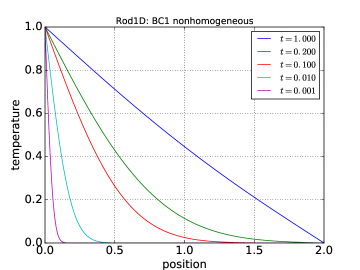
Figure 12: BC1 for $\kappa=1$, $L=2$, $T_{1}=1$, $T_{2}=0$ ($\alpha_{1}=1,\beta_{1}=0,\gamma_{1}=1$, and $\alpha_{1}=1,\beta_{1}=0,\gamma_{1}=0$), with $T_{\rm\scriptscriptstyle L}=0$, $T_{\rm\scriptscriptstyle R}=0$. Solver instantiation: Rod1D(alpha1=1, beta1=0, alpha2=1, gamma1=1, beta2=0, gamma2=0, TL=0, TR=0).

For Fig. 12, the Class Rod1D takes the boundary and initial condition arguments

Rod1D(alpha1=1, beta1=0, gamma1=1, alpha2=1,beta2=0, gamma2=0, TL=0, TR=0).

Note that $T_{1}=\gamma_{1}/\alpha_{1}=1$ and $T_{2}=\gamma_{2}/\alpha_{2}=0$.

IV.1.2 BC2

For the boundary conditions

$$\partial_{x}T(0,t) = F$$ (192)

$$\partial_{x}T(L,t) = F\ ,$$ (193)

the full nonhomogeneous solution is thus

$$T(x,t) = Fx+\frac{A_{0}}{2}+\sum_{n=1}^{\infty}A_{n}\,\cos k_{n}x\,e^{-\kappa\,k_{n}^{2}t}\ .$$ (194)

Using the initial condition $T(x,t=0)=T_{0}(x)$, we find

$$\frac{A_{0}}{2}+\sum_{n=1}^{\infty}A_{n}\,\cos k_{n}x = T_{0}(x)-Fx=T_{\rm\scriptscriptstyle L}+\frac{(T_{\rm\scriptscriptstyle R}-FL)-T_{\rm\scriptscriptstyle L}}{L}\,x\ .$$ (195)

We can use the previous results (197) and (198) provided we make the substitution $T_{\rm\scriptscriptstyle L}\to T_{a}=T_{\rm\scriptscriptstyle L}$ and $T_{\rm\scriptscriptstyle R}\to T_{b}=T_{\rm\scriptscriptstyle R}-FL$,

$$T_{a} = T_{\rm\scriptscriptstyle L}\hskip 14.22636ptT_{b}=T_{\rm\scriptscriptstyle R}-FL$$ (196)

$$\frac{A_{0}}{2} = \frac{1}{2}\Big{(}T_{a}+T_{b}\Big{)}$$ (197)

$$A_{n} = 2\,\Big{(}T_{a}-T_{b}\Big{)}\,\frac{1-(-1)^{n}}{n^{2}\pi^{2}}\ .$$ (198)

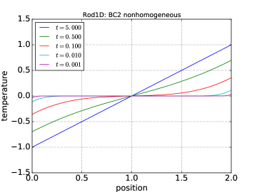
Figure 13: BC2 with $\kappa=1$, $L=2$, $F=1$ (with $T_{\rm\scriptscriptstyle L}=0$, $T_{\rm\scriptscriptstyle R}=0$). ExactPack instantiation: Rod1D(alpha1=0, beta1=1, gamma1=F, alpha2=0, beta2=1, gamma2=F, TL=0, TR=0).

The instantiation of Rod1D used for Fig. 13 is

Rod1D(alpha1=1, beta1=0, alpha2=1, gamma1=1, beta2=0, gamma2=0, TL=0, TR=0).

Since $T_{1}=\gamma_{1}/\alpha_{1}$, and $T_{2}=\gamma_{2}/\alpha_{2}$, we could simplify the interface to

PlanarSandwich(TL=T1, TR=T2, Nsum=1000).

IV.1.3 BC3

For the boundary conditions

$$T(0,t) = T_{1}$$ (199)

$$\partial_{x}T(L,t) = F_{2}\ ,$$ (200)

the full nonhomogeneous solution is thus

$$T(x,t) = T_{1}+\frac{T_{2}-T_{1}}{L}\,x+\sum_{n=0}^{\infty}B_{n}\,\sin k_{n}x\,e^{-\kappa\,k_{n}^{2}t}$$ (201)

$$T_{2} = T_{1}+F_{2}L=\frac{\gamma_{1}}{\alpha_{1}}+\frac{\gamma_{2}L}{\beta_{2}}$$ (202)

$$k_{n} = \frac{(2n+1)\pi}{2L}\hskip 28.45274ptn=0,1,2,\cdots\ .$$ (203)

The Fourier coefficients

$$B_{n}=\frac{2}{L}\,\int_{0}^{L}dx\,\Big{[}T_{0}(x)-\bar{T}(x)\Big{]}\sin k_{n}x$$ (204)

take the form

$$B_{n} = \frac{4T_{a}}{(2n+1)\pi}+4\big{(}T_{b}-T_{a}\big{)}\left[\frac{1}{(2n+1)\pi}-\frac{2}{(2n+1)^{2}\pi^{2}}\right]$$ (205)

$$= \frac{4T_{b}}{(2n+1)\pi}-\frac{8\big{(}T_{b}-T_{a}\big{)}}{(2n+1)^{2}\pi^{2}}\ .$$ (206)

IV.1.4 BC4

For the boundary conditions

$$\partial_{x}T(0,t) = F_{1}$$ (207)

$$T(L,t) = T_{2}\ ,$$ (208)

the full nonhomogeneous solution is

$$\bar{T}(x) = T_{1}+\frac{T_{2}-T_{1}}{L}\,x+\sum_{n=0}^{\infty}A_{n}\,\cos k_{n}x\,e^{-\kappa\,k_{n}^{2}t}$$ (209)

$$T_{1} = T_{2}-F_{1}L=\frac{\gamma_{2}}{\alpha_{2}}-\frac{\gamma_{1}L}{\beta_{1}}$$ (210)

$$k_{n} = \frac{(2n+1)\pi}{2L}\hskip 28.45274ptn=0,1,2,\cdots\ .$$ (211)

As before, we take the linear initial condition (15), and then (77) gives the coefficients

$$A_{n} = 4T_{a}\,\frac{(-1)^{n}}{(2n+1)\pi}-8\Big{(}T_{b}-T_{a}\Big{)}\,\frac{1-(-1)^{n}}{(2n+1)^{2}\,\pi^{2}}\ .$$ (212)

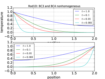
Figure 14: BC3 and BC4 for $\kappa=1$, $L=2$, $T_{1}=1,T_{2}=0$, $T_{\rm\scriptscriptstyle L}=T_{\rm\scriptscriptstyle R}=0$. The two profiles should be mirror images of each other, by symmetry principle. This appears to be the case, for for $N_{\rm max}=300$. Note that the profile are indeed asymmetric. BC3: Rod1D(alpha1=1, beta1=0, alpha2=0, beta2=1, TL=3, TR=4). BC4: Rod1D(alpha1=0, beta1=1, alpha2=1, beta2=0, TL=4, TR=3).

IV.2 General Boundary Conditions

For general boundary conditions, the full nonhomogeneous solution is

$$T(x,t) = T_{1}+\frac{T_{2}-T_{1}}{L}\,x+\sum_{n=1}^{\infty}D_{n}\,X_{n}(x)\,e^{-\kappa\,k_{n}^{2}t}$$ (213)

$$X_{n}(x) = A_{n}\cos k_{n}x+B_{n}\sin k_{n}x\ ,$$ (214)

with coefficients

$$A_{n} = -\frac{\beta_{1}k_{n}}{\alpha_{1}}\,B_{n}$$ (215)

$$T_{1} = \frac{\beta_{2}\gamma_{1}-\beta_{1}\gamma_{2}+L\alpha_{2}\gamma_{1}}{\alpha_{1}\beta_{2}-\alpha_{2}\beta_{1}+L\alpha_{1}\alpha_{2}}$$ (216)

$$T_{2} = \frac{\beta_{2}\gamma_{1}-\beta_{1}\gamma_{2}+L\alpha_{1}\gamma_{2}}{\alpha_{1}\beta_{2}-\alpha_{2}\beta_{1}+L\alpha_{1}\alpha_{2}}\ .$$ (217)

The Fourier coefficients are

$$D_{n} = \frac{1}{N_{n}}\int_{0}^{L}dx\,\Big{[}T_{0}(x)-\bar{T}(x)\Big{]}X_{n}(x)\ .$$ (218)

The zeroth order contributions is $T_{0}^{(0)}(x)-\bar{T}^{(0)}(x)=T_{a}$, and we find

$$D_{n}^{(0)} = \frac{T_{a}}{N_{n}}\,\left[\frac{1-\cos k_{n}L}{k_{n}}-\frac{\beta_{1}\sin k_{n}L}{\alpha_{1}}\right]\ .$$ (219)

The first order contribution is $T_{0}^{(1)}(x)-\bar{T}^{(0)}(x)=(T_{b}-T_{a})\,x/L$ we have

$$D_{n}^{(1)} = \frac{T_{b}-T_{a}}{N_{n}\,L}\,\frac{1}{\alpha_{1}k_{n}^{2}}\,\Big{[}\beta_{1}k_{n}-(\alpha_{1}k_{n}L+\beta_{1}k_{n})\cos k_{n}L+(\alpha_{1}-\beta_{1}k_{n}^{2}L)\sin k_{n}L\Big{]}\ .$$ (220)

The normalization factor is

$$N_{n}=\frac{1}{4k_{n}\alpha_{1}^{2}}\Big{[}-2\alpha_{1}\beta_{1}k_{n}+2(\beta_{1}^{2}k_{n}^{2}+\alpha_{1}^{2})k_{n}L+2\alpha_{1}\beta_{1}k_{n}\cos 2k_{n}L+(\beta_{1}^{2}k_{n}^{2}-\alpha_{1}^{2})\sin 2k_{n}L\Big{]}$$

$$\ .$$ (221)

Setting $\mu\equiv kL$ and $\bar{\beta}_{i}\equiv\beta_{i}/L$, we can write (142) in the form

$$\tan\mu = \frac{(\alpha_{2}\bar{\beta}_{1}-\alpha_{1}\bar{\beta}_{2})\,\mu}{\alpha_{1}\alpha_{2}+\bar{\beta}_{1}\bar{\beta}_{2}\,\mu^{2}}\ .$$ (222)

Equation (222) will give solutions $\mu_{n}$ for $n=0,1,2,\cdots$ (with $\mu_{0}=0)$, and the wave numbers become

$$k_{n}=\frac{\mu_{n}}{L}\ .$$ (223)

Appendix A Sample ExactPack Script

The following script produces Fig. 2.

import numpy as np
import matplotlib.pylab as plt

from exactpack.solvers.heat import PlanarSandwich

L = 2.0
x = np.linspace(0.0, L, 1000)
t0 = 1.0
t1 = 0.2
t2 = 0.1
t3 = 0.01
t4 = 0.001

solver = PlanarSandwich(T1=1, T2=0, L=L, Nsum=1000)
soln0 = solver(x, t0)
soln1 = solver(x, t1)
soln2 = solver(x, t2)
soln3 = solver(x, t3)
soln4 = solver(x, t4)
soln0.plot(’temperature’, label=r’$t=1.000$’)
soln1.plot(’temperature’, label=r’$t=0.200$’)
soln2.plot(’temperature’, label=r’$t=0.100$’)
soln3.plot(’temperature’, label=r’$t=0.010$’)
soln4.plot(’temperature’, label=r’$t=0.001$’)

plt.title(’Planar Sandwich’)
plt.ylim(0,1)
plt.xlim(0,L)
plt.legend(loc=0)
plt.grid(True)
plt.show()

Appendix B Uniformly Convergent Sequences of Functions

Many of the mathematical operations we take for granted in a typical analytic calculation of a physical process, such as the simple interchange of a limit and an integral, depend deeply upon issues surrounding the uniform convergence of sequences of functions. By way of introduction, let us consider a solution $T(x,t)$ to the heat flow equations (1)–(4). Let us further consider a sequence of times $t_{1},t_{2},t_{3},\cdots$, from which we can construct a sequence of temperature profiles $T_{n}(x)=T(x,t_{n})$. In other words, $T_{n}(x)$ is a sequence of functions of $x$, indexed by the integers $n$, or equivalently by the times $t_{n}$. Suppose now that the time sequence $t_{n}$ converges to the limit $t_{0}$, so that $\lim_{n\to\infty}t_{n}=t_{0}$. Then, for our purposes, we may speak interchangeably of the limits $\lim_{n\to\infty}T_{n}(x)$ and $\lim_{t\to t_{0}}T(x,t)$, and in this way, we can think of $T(x,t)$ as a sequence of functions of $x$ indexed by $t$. To make this more precise, and to refresh our memories, it is constructive to review the formal definition of a limit. The sequence $\{t_{n}\}$ converges to the the limit $t_{0}$ as $n\to\infty$, denoted

$$\lim_{n\to\infty}t_{n}=t_{0}\ ,$$ (224)

provided that for every $\epsilon>0$ there exists $N>0$ such that

$$\big{|}t_{n}(x)-t_{0}\big{|}<\epsilon$$ (225)

whenever $n\geq N$. That is to say, $t_{n}$ can be made arbitrarily close to $t_{0}$ by choosing $n$ arbitrarily large.

The notion of a limit can extended to a sequence of functions. The domain of the functions $T_{n}(x)$, which we refer to as $E$, can be either the open interval $(0,L)$, or the closed interval $[0,L]$, if we are also interested in the boundary points $x=0,L$. For definiteness, we take the case BC1, for which $T(0,t_{n})=T_{1}$ and $T(L,t_{n})=T_{2}$. There are two distinct (but related) sense in which the limit

$$\lim_{n\to\infty}T_{n}(x)=T(x)$$ (226)

exists. The obvious way to interpret this limit is to choose a value of $x=x_{0}$, and to take the limit of the normal sequence of numbers $T_{1}(x_{0}),T_{2}(x_{0}),T_{3}(x_{0}),\cdots$. If, in the limit $n\to\infty$, the sequence converges to a number $T(x_{0})$ for some function $T(x)$, we say that the sequence $T_{n}(x)$ converges point-wise to $T(x)$ at $x=x_{0}$. This is made formal by the following definition.

Definition: The sequence of functions $\{T_{n}(x)\}$ converges point-wise on $E$ to a function $T(x)$ if for every $x\in E$ and for every $\epsilon>0$ there is an integer $N$ such that

$$\big{|}T_{n}(x)-T(x)\big{|}<\epsilon$$ (227)

for all $n\geq N$.

The integer $N$ might depend upon the point $x$. If, however, we can choose the same $N$ for all $x\in E$, then we say that the limit is uniformly convergent. This is made precise in following definition.

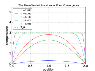
Figure 15: Temperature profiles for the homogeneous planar sandwich at times $t_{1}=1$, $t_{2}=0.2$, $t_{3}=0.1$, $t_{4}=0.01$, and $t_{5}=0.001$. The diffusion constant is $\kappa=1$ and length of the rod is $L=2$, with a constant initial condition $T_{0}(x)=3$. The plot uses the instance PlanarSandwich(T1=0, T2=0, TL=3, TR=3, L=2, Nsum=1000). Since the boundary conditions are incommensurate with the initial condition, the solution $T(y,t)$ convergens non-uniformly on the open $x$-interval $(0,L)$ to $T_{0}(x)=3$, which is plotted by the dashed line.

Definition: The sequence of functions $\{T_{n}(x)\}$ converges uniformly on $E$ to a function $T(x)$ if for every $\epsilon>0$ there is an integer $N$ such that

$$\big{|}T_{n}(x)-T(x)\big{|}<\epsilon$$ (228)

for all $n\geq N$ and all $x\in E$.

As an example, let us consider the solution illustrated in Fig. 15. This is a homogeneous solution, for which $T(0,t)=T(0,L)=0$, with a constant initial condition $T_{0}(x)=3$ (for $0<x<L$). The time sequence is $t_{1}=1$, $t_{2}=0.2$, $t_{3}=0.1$, $t_{4}=0.01$, $t_{5}=0.001,\cdots$. We see that $\lim_{n\to\infty}T_{n}(x)=T_{0}(x)$ for $x\in(0,L)$, but the limit is non-uniform.

References

- (1) ExactPack source code, https://github.com/lanl/ExactPack (formally github.com/losalamos), LA-CC-14-047.
- (2) A Dawes, C Malone, M Shashkov, Some New Verification Test Problems for Multimaterial Diffusion on Meshes that are Non-Aligned with Material Boundaries, LA-UR-16-24696, Los Alamos report (2016).
- (3) Paul W Berg and James L McGregor, Elementary Partial Differential Equations, Holden Day (1966).
- (4) Walter Rubin, Principles of Mathematical Analysis, McGraw-Hill, third edition (1976).