Scattering of a diatomic composite system

Abstract

We investigate the scattering problem of a two-particle composite system on a delta-function potential. Using the time independent scattering theory, we study how the transmission/reflection coefficients change with the height of external potential, the incident momentum, and the strength of internal potential. In particular, we show that the existence of internal degree of freedom can significantly change the transmission/reflection coefficients even without internal excitation. We consider two scenarios: the internal degree of freedom of the incident wave is set to be in a state with even parity or odd parity, we find that the influence of a symmetric Hamiltonian is greater on the odd-parity internal states than on the even-parity ones.

I Introduction

The quantum superposition principle lies at the heart of quantum mechanics and allows massive objects to be prepared in spatial superposition of the order of their sizes. Although quantum interferences of macroscopic objects have remaind experimentally challenging ORom ; ABas , a series of preparatory work  WMar ; ORome ; ORomer ; TKov ; UBHo ; JQLi ; MCar ; MAbd have been finished. Experiments involving composite systems WSch ; MArn ; SGer provide a way to probe the quantum interferences of macroscopic objects, moreover, it requires controlled splitting of a wave pocket to observe interference. In our model, we simulate this process by employing a delta-function potential to separate the incoming wave into two (reflected and transmitted) components. As a composite system that contains two particles at least, the energy levels of the internal degree of freedom may be excited. In the following, we consider a diatomic bound system and exhibit how the internal states affect the reflected and transmitted components.

As a good approximation to many actual phenomena, quantum mechanical scattering in one dimension attracts increasing interest during the past years LLSa ; AMos1 ; WTrz ; LVChe ; MGRo ; LVCh ; FQue . Scattering theory JRTa ; RGNe promotes greatly the experimental research on the interaction and internal structure of particles. The elegance and power of the $S$-matrix formulation is beyond doubt, but this formulation always has high computation complexity, especially for the higher-order correction. In this paper, we propose a simple method to calculate the probability that a composite system that entered the collision with in asymptote state will be observed to emerge with out asymptote state. $S$-matrix within Born approximate is also calculated to compare with our proposal.

In our study, we discuss the scattering process of a two-particle bound system to mimic the splitting of the incoming wave corresponding to a diatomic composite system. The coefficients of reflection and transmission for different internal modes are worked out by invoking appropriate boundary conditions on the eigenfunctions of the Hamiltonian, but not by calculating the high-order correction of $S$-matrix elements. In the following, we will see the condition that excited internal modes become populated and their influence on the reflected and transmitted components. We propose our model in section II and list the results in section III, in section IV, we end with a summary.

II Theoretical Model

Consider two particles with mass $m_{1},m_{2}$ and coordinates $x_{1},x_{2}$. A model which resembles the interaction of these particles and the scattering potential is specified by the Hamiltonian

$$H=-\frac{\hbar^{2}}{2m_{1}}\partialderivative[2]{x_{1}}-\frac{\hbar^{2}}{2m_{2}}\partialderivative[2]{x_{2}}+\Omega^{2}{(x_{1}-x_{2})}^{2}+\gamma_{1}\delta(x_{1})+\gamma_{2}\delta(x_{2}),$$ (1)

where we assume that the particles are tied to each other by a harmonic coupling with stiffness $\Omega$ and the scattering potential has the form $V(x_{i})=\gamma_{i}\delta(x_{i})$.

For convenience, we rewrite the Hamiltonian in terms of center-of-mass coordinate $X=(m_{1}x_{1}+m_{2}x_{2})/(m_{1}+m_{2})$ and relative coordinate $x=x_{2}-x_{1}$

$$H=-\frac{\hbar^{2}}{2M}\partialderivative[2]{X}-\frac{\hbar^{2}}{2\mu}\partialderivative[2]{x}+\frac{1}{2}\mu\omega^{2}x^{2}+\gamma_{1}\delta(X-r_{2}x)+\gamma_{2}\delta(X+r_{1}x),$$ (2)

where $M=m_{1}+m_{2}$, $\mu=m_{1}m_{2}/M$, $r_{i}=m_{i}/M$.

Obviously, the eigenstates of $H_{0}=-\hbar^{2}\partialderivative[2]{X}/2M-\hbar^{2}\partialderivative[2]{x}/2\mu+\mu\omega^{2}x^{2}/2$ are

$$\phi_{K,n}(X,x)=\frac{1}{\sqrt{2\pi}}e^{iKX}\psi_{n}(x),$$ (3)

for $n=0,1,2...$ with eigenenergies

$$E_{K,n}=\frac{\hbar^{2}K^{2}}{2M}+\left(n+\frac{1}{2}\right)\hbar\omega,$$ (4)

where $K$ denotes the momentum of the center-of-mass and $\{\psi_{n}(x)\}$ are the normalized stationary wave functions for harmonic oscillator and they describe the internal states of this bound system. If the system is incoming from the left (as shown in Fig. 1) with momentum $K_{0}$ and the internal degree of freedom is assumed to be in the $l$-th state, the scattering state reads

$$\Psi_{K_{0},l}^{+} = \begin{cases}\phi_{K_{0},l}+\sum_{n}\alpha_{n}\phi_{-K_{n},n},&x_{1}<0,x_{2}<0\\ \sum_{n}\mu_{n}\phi_{K_{n},n}+\sum_{n}\nu_{n}\phi_{-K_{n},n},&x_{1}<0,x_{2}>0\\ \sum_{n}\xi_{n}\phi_{K_{n},n}+\sum_{n}\eta_{n}\phi_{-K_{n},n},&x_{1}>0,x_{2}<0\\ \sum_{n}\beta_{n}\phi_{K_{n},n},&x_{1}>0,x_{2}>0\end{cases}$$ (5)

where $\{\alpha_{n},\beta_{n}\}$ are the amplitudes of different modes for the reflected and transmitted waves respectively, $K_{n}$ are the momentum of the center-of-mass corresponding to the $n$-th internal state and can be derived from the energy conservation condition:

$$\frac{\hbar^{2}K_{0}^{2}}{2M}+(l+\frac{1}{2})\hbar\omega=\frac{\hbar^{2}K_{n}^{2}}{2M}+(n+\frac{1}{2})\hbar\omega.$$ (6)

Furthermore, we can easily get the probability current densities of incident, reflected and transmitted waves with different modes

$$J_{0}^{in} =\frac{1}{2\pi}\frac{\hbar K_{0}}{M},$$ (7)

$$J_{n}^{re} =-\frac{|\alpha_{n}|^{2}}{2\pi}\frac{\hbar K_{n}}{M},$$ (8)

$$J_{n}^{tr} =\frac{|\beta_{n}|^{2}}{2\pi}\frac{\hbar K_{n}}{M}.$$ (9)

Thus the corresponding coefficients of reflection and transmission are

$$j_{n}^{re} =\frac{|J_{n}^{re}|}{J_{0}^{in}}=|\alpha_{n}|^{2}\frac{K_{n}}{K_{0}},$$ (10)

$$j_{n}^{tr} =\frac{J_{n}^{tr}}{J_{0}^{in}}=|\beta_{n}|^{2}\frac{K_{n}}{K_{0}}.$$ (11)

Note that the conservation of probability implies

$$j_{t}=\sum_{n}\left(j_{n}^{re}+j_{n}^{tr}\right)=1.$$ (12)

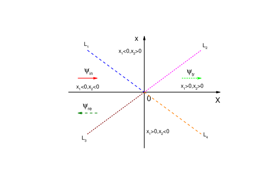
Figure 1: (Color online) Schematic scattering process in the $X-x$ frame. The scattering potentials locate along $x_{1}=0$ (i.e., $L_{2}$ and $L_{3}$) and $x_{2}=0$ (i.e., $L_{1}$ and $L_{4}$), and an incoming wave is separated into a reflected and a transmitted component.

The boundary conditions at $x_{1}=0$ and $x_{2}=0$ require

$$\begin{cases}\hskip 96.73918pt\Psi_{K_{0},l}^{+}|_{x_{1}\rightarrow 0^{+}}&=\Psi_{K_{0},l}^{+}|_{x_{1}\rightarrow 0^{-}},\\ \partialderivative{x_{1}}{\Psi_{K_{0},l}^{+}|_{x_{1}\rightarrow 0^{+}}}-\partialderivative{x_{1}}{\Psi_{K_{0},l}^{+}|_{x_{1}\rightarrow 0^{-}}}&=\frac{2m_{1}\gamma_{1}}{\hbar^{2}}\Psi_{K_{0},l}^{+}|_{x_{1}\rightarrow 0^{+}},\\ \hskip 96.73918pt\Psi_{K_{0},l}^{+}|_{x_{2}\rightarrow 0^{+}}&=\Psi_{K_{0},l}^{+}|_{x_{2}\rightarrow 0^{-}},\\ \partialderivative{x_{2}}{\Psi_{K_{0},l}^{+}|_{x_{2}\rightarrow 0^{+}}}-\partialderivative{x_{2}}{\Psi_{K_{0},l}^{+}|_{x_{2}\rightarrow 0^{-}}}&=\frac{2m_{2}\gamma_{2}}{\hbar^{2}}\Psi_{K_{0},l}^{+}|_{x_{2}\rightarrow 0^{+}},\end{cases}$$ (13)

Concretely speaking, the continuity of the wave function at $L_{1}$ (see Fig. 1) gives

$$e^{iK_{0}r_{1}x_{1}}\psi_{l}(-x_{1})+\sum_{n}\alpha_{n}e^{-iK_{n}r_{1}x_{1}}\psi_{n}(-x_{1})$$

$$=\sum_{n}\mu_{n}e^{iK_{n}r_{1}x_{1}}\psi_{n}(-x_{1})+\sum_{n}\nu_{n}e^{-iK_{n}r_{1}x_{1}}\psi_{n}(-x_{1}),$$

$$\hskip 170.71652pt(x_{1}<0)$$ (14)

and the discontinuity of the derivative of wave function at $L_{1}$ gives

$$\frac{2m_{2}\gamma_{2}}{\hbar^{2}}\left[\sum_{n}\mu_{n}e^{iK_{n}r_{1}x_{1}}\psi_{n}(-x_{1})+\sum_{n}\nu_{n}e^{-iK_{n}r_{1}x_{1}}\psi_{n}(-x_{1})\right]$$

$$=\sum_{n}\mu_{n}\left[e^{iK_{n}r_{1}x_{1}}\psi_{n}^{{}^{\prime}}(-x_{1})+iK_{n}r_{2}e^{iK_{n}r_{1}x_{1}}\psi_{n}(-x_{1})\right]$$

$$\quad{}+\sum_{n}\nu_{n}\left[e^{-iK_{n}r_{1}x_{1}}\psi_{n}^{{}^{\prime}}(-x_{1})-iK_{n}r_{2}e^{-iK_{n}r_{1}x_{1}}\psi_{n}(-x_{1})\right]$$

$$\quad{}-\left[e^{iK_{0}r_{1}x_{1}}\psi_{0}^{{}^{\prime}}(-x_{1})+e^{iK_{0}r_{1}x_{1}}iK_{0}r_{2}\psi_{0}(-x_{1})\right]$$

$$\quad{}-\sum_{n}\alpha_{n}\left[e^{-iK_{n}r_{1}x_{1}}\psi_{n}^{{}^{\prime}}(-x_{1})-iK_{n}r_{2}e^{-iK_{n}r_{1}x_{1}}\psi_{n}(-x_{1})\right]$$

$$\hskip 170.71652pt(x_{1}<0).$$ (15)

Multiplying Eq. 14 and Eq. 15 with $\psi_{m}$ and integrating from $0$ to $\infty$ leads to

$$c_{ml}^{2}(-iK_{0}r_{1})+\sum_{n}\alpha_{n}c_{mn}^{2}(iK_{n}r_{1})$$

$$=\sum_{n}\mu_{n}c_{mn}^{2}(-iK_{n}r_{1})+\sum_{n}\nu_{n}c_{mn}^{2}(iK_{n}r_{1})$$ (16)

and

$$\frac{2m_{2}\gamma_{2}}{\hbar^{2}}\left[\sum_{n}\mu_{n}c_{mn}^{2}(-iK_{n}r_{1})+\sum_{n}\nu_{n}c_{mn}^{2}(iK_{n}r_{1})\right]$$

$$=\sum_{n}\mu_{n}\left[iK_{n}r_{2}c_{mn}^{2}(-iK_{n}r_{1})+d_{mn}^{2}(-iK_{n}r_{1})\right]$$

$$\quad{}+\sum_{n}\nu_{n}\left[-iK_{n}r_{2}c_{mn}^{2}(iK_{n}r_{1})+d_{mn}^{2}(iK_{n}r_{1})\right]$$

$$\quad{}-\left[iK_{0}r_{2}c_{ml}^{2}(-iK_{0}r_{1})+d_{ml}^{2}(-iK_{0}r_{1})\right]$$

$$\quad{}-\sum_{n}\alpha_{n}\left[-iK_{n}r_{2}c_{mn}^{2}(iK_{n}r_{1})+d_{mn}^{2}(iK_{n}r_{1})\right].$$ (17)

Similarly, the boundary conditions at $L_{2}$, $L_{3}$ and $L_{4}$ take the form

$$\sum_{n}\mu_{n}c_{mn}^{2}(iK_{n}r_{2})+\sum_{n}\nu_{n}c_{mn}^{2}(-iK_{n}r_{2})$$

$$=\sum_{n}\beta_{n}c_{mn}^{2}(iK_{n}r_{2}),$$ (18)

$$\frac{2m_{1}\gamma_{1}}{\hbar^{2}}\sum_{n}\beta_{n}c_{mn}^{2}(ik_{n}r_{2})$$

$$=\sum_{n}\beta_{n}\left[iK_{n}r_{1}c_{mn}^{2}(iK_{n}r_{2})-d_{mn}^{2}(iK_{n}r_{2})\right]$$

$$\quad{}-\sum_{n}\mu_{n}\left[iK_{n}r_{1}c_{mn}^{2}(iK_{n}r_{2})-d_{mn}^{2}(iK_{n}r_{2})\right]$$

$$\quad{}-\sum_{n}\nu_{n}\left[-iK_{n}r_{1}c_{mn}^{2}(-iK_{n}r_{2})-d_{mn}^{2}(-iK_{n}r_{2})\right],$$ (19)

$$c_{ml}^{1}(iK_{0}r_{2})+\sum_{n}\alpha_{n}c_{mn}^{1}(-iK_{n}r_{2})$$

$$=\sum_{n}\xi_{n}c_{mn}^{1}(iK_{n}r_{2})+\sum_{n}\eta_{n}c_{mn}^{1}(-iK_{n}r_{2}),$$ (20)

$$\frac{2m_{1}\gamma_{1}}{\hbar^{2}}\left[\sum_{n}\xi_{n}c_{mn}^{1}(iK_{n}r_{2})+\sum_{n}\eta_{n}c_{mn}^{1}(-ik_{n}r_{2})\right]$$

$$=\sum_{n}\xi_{n}\left[iK_{n}r_{1}c_{mn}^{1}(iK_{n}r_{2})-d_{mn}^{1}(iK_{n}r_{2})\right]$$

$$\quad{}+\sum_{n}\eta_{n}\left[-iK_{n}r_{1}c_{mn}^{1}(-iK_{n}r_{2})-d_{mn}^{1}(-iK_{n}r_{2})\right]$$

$$\quad{}-\left[iK_{0}r_{1}c_{ml}^{1}(iK_{0}r_{2})-d_{ml}^{1}(iK_{0}r_{2})\right]$$

$$\quad{}-\sum_{n}\alpha_{n}\left[-iK_{n}r_{1}c_{mn}^{1}(-iK_{n}r_{2})-d_{mn}^{1}(-iK_{n}r_{2})\right],$$ (21)

$$\sum_{n}\xi_{n}c_{mn}^{1}(-iK_{n}r_{1})+\sum_{n}\eta_{n}c_{mn}^{1}(iK_{n}r_{1})$$

$$=\sum_{n}\beta_{n}c_{mn}^{1}(-iK_{n}r_{1}),$$ (22)

and

$$\frac{2m_{2}\gamma_{2}}{\hbar^{2}}\sum_{n}\beta_{n}c_{mn}^{1}(-iK_{n}r_{1})$$

$$=\sum_{n}\beta_{n}\left[iK_{n}r_{2}c_{mn}^{1}(-iK_{n}r_{1})+d_{mn}^{1}(-iK_{n}r_{1})\right]$$

$$\quad{}-\sum_{n}\xi_{n}\left[iK_{n}r_{2}c_{mn}^{1}(-iK_{n}r_{1})+d_{mn}^{1}(-iK_{n}r_{1})\right]$$

$$\quad{}-\sum_{n}\eta_{n}\left[-iK_{n}r_{2}c_{mn}^{1}(iK_{n}r_{1})+d_{mn}^{1}(iK_{n}r_{1})\right],$$ (23)

where $c_{mn}^{1}(q)=\int_{-\infty}^{0}\psi_{m}(x)e^{qx}\psi_{n}(x)\mathbf{d}x$, $c_{mn}^{2}(q)=\int_{0}^{\infty}\psi_{m}(x)e^{qx}\psi_{n}(x)\mathbf{d}x$, $d_{mn}^{1}(q)=\int_{-\infty}^{0}\psi_{m}(x)e^{qx}\psi_{n}^{{}^{\prime}}(x)\mathbf{d}x$ and $d_{mn}^{2}(q)=\int_{0}^{\infty}\psi_{m}(x)e^{qx}\psi_{n}^{{}^{\prime}}(x)\mathbf{d}x$.

Eqs.16$-$23 determine $\Psi_{K_{0},l}^{+}$. In the following we will analyze the scattering behavior of this two-particle composite system.

III Results and Analysis

In this section, we calculate how the population of excited states changes with different parameters, and analyze the physical picture behind it. In the following calculation, we set $\hbar=1$, $M=2$ and select the incident internal state to be the ground state or the first excited state, i.e., $l=0$ or $1$.

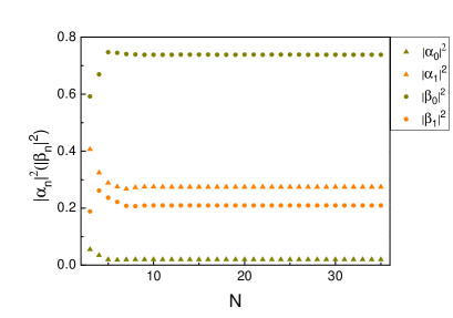
(a)

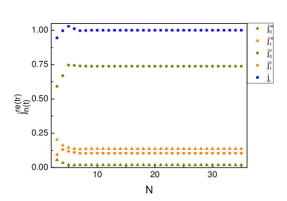
(b)

Figure 2: (Color online) The amplitudes $\alpha_{n},\beta_{n}$ (a) and reflection/transmission coefficients $j_{n}$ (b) via the total modes $N$ with parameters $K_{0}=4$, $\omega=3$, $\gamma_{1}=1$, $\gamma_{2}=0$ and $n_{c}=1$.

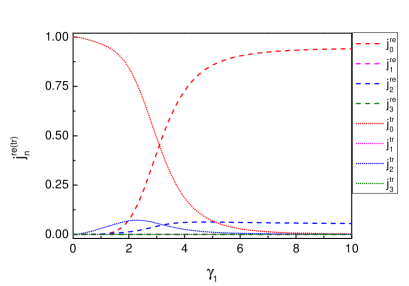
(a)

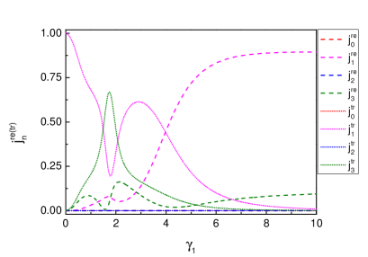
(b)

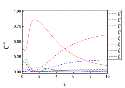
(c)

Figure 3: (Color online) The reflection/transmission coefficients $j_{n}$ via the potential strength $\gamma_{1}$ with parameters (a) $m_{1}=1$, $K_{0}=5.2$, $\omega=2$, $\gamma_{2}=\gamma_{1},l=0$; (b) $m_{1}=1$, $K_{0}=4.5$, $\omega=2$, $\gamma_{2}=\gamma_{1},l=1$; (c) $m_{1}=1.1$, $K_{0}=5.2$, $\omega=2$, $\gamma_{2}=2,l=0$.

From Eq. 6, it’s reasonable to believe that: (1) the $n$-th excited internal state may become populated if its energy is less than the energy of the incident wave $(n+1/2)\hbar\omega\leq\hbar^{2}K_{0}^{2}/2M+(l+1/2)\hbar\omega$; (2) the highest internal energy level excited by the potential should be $n_{c}=\lfloor\hbar K_{0}^{2}/(2M\omega)\rfloor+l$, where $\lfloor a\rfloor$ is the maximum integer less than or equal to $a$. However it is worthy to point out that in Eqs.16$-$23, the levels above $n_{c}$ should also be taken into account to ensure the conservation of probability is satisfied, thus $K_{n}=i\sqrt{2nM\omega-K_{0}^{2}}$ for $n>n_{c}$. These correspond to the states whose internal energies are sufficiently high while the center-of-mass energies being negative. From the point of physics, these sates only exist in the scattering region since they decay rapidly as $|X|\rightarrow\infty$. In fact, it’s enough to take only several internal modes above $n_{c}$ into account. Fig. 2 shows that the results are stable with the increasing of the mode number, indicating that the modes well above $n_{c}$ have little effect on the population of the actual states.

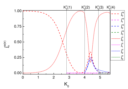
(a)

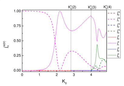
(b)

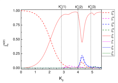
(c)

Figure 4: (Color online) The reflection/transmission coefficients $j_{n}$ via the incident momentum of the center-of-mass $K_{0}$ with parameters (a) $m_{1}=1$, $\omega=2$, $\gamma_{1}=\gamma_{2}=1,l=0$; (b) $m_{1}=1$, $\omega=2$, $\gamma_{1}=\gamma_{2}=1,l=1$; (c) $m_{1}=1.1$, $\omega=2$, $\gamma_{1}=0.8,\gamma_{2}=0.5,l=0$.

The influences of barrier heights $\gamma_{1,2}$ are different for the reflected and transmitted part of the wave. As a consequence, the internal modes become populated differently. As shown in Fig. 3a and Fig. 3b, in the limit $\gamma_{1}=\gamma_{2}=0$, the incident wave $\phi_{K_{0},l}$ transmits directly without reflection and excitation ($j_{l}^{tr}=1$). For $l=0$ (Fig. 3a), with the increasing of $\gamma_{1}$, the transmission coefficient for ground mode $j_{0}^{tr}$ decreases monotonously while the reflection coefficient $j_{0}^{re}$ increases. It should be stressed that, at the quite beginning of $\gamma_{1}$, the reflection/transmission coefficients for excited states $j_{2}^{re(tr)}$ increase, indicating that a certain height of potential is needed to excite the upper states. With the further increasing of $\gamma_{1}$, $j_{n}^{re}$ increase and $j_{n}^{tr}$ decrease, only reflected components remains for the potential high enough.

We want to emphasize that the influence of a symmetric Hamiltonian( i.e., $m_{1}=m_{2},\gamma_{1}=\gamma_{2}$) is greater on the odd-parity internal states than on the even-parity ones. The curves of $j_{1,3}$ in Fig. 3b have obviously characteristics ”peak” and ”valley” which are not available for $j_{0,2}$ in Fig. 3a. Moreover, Fig. 3 illustrates the dependence of the internal excitation on the symmetry of Hamiltonian. The internal degree of freedom can only be excited to the states whose parity is same as that of the incident state for a symmetric Hamiltonian, (Fig. 3a, Fig. 3b), contrasting to that all the states $n\leq n_{c}$ could be excited for a asymmetric Hamiltonian $m_{1}\neq m_{2}$,$\gamma_{1}\neq\gamma_{2}$ (Fig. 3c).

From Eq. 6, the critical incident momentums which could excite $n$-th internal states read

$$K_{0}^{c}(n)=\sqrt{2(n-l)M\omega/\hbar},$$ (24)

if $K_{0}>K_{0}^{c}(n)$, the $n$-th internal state may be excited. This is the energy condition to excite internal states. Fig. 4 displays how reflection and transmission coefficients $j_{n}$ change with $K_{0}$, the vertical lines label $K_{0}^{c}$ to excite $n=1,2,3$ states. For $l=0$ (Fig. 4a), when $K_{0}$ is not too large, the internal degree of freedom is in the ground state, the reflection (transmission) coefficient decreases (increases) with the increasing of $K_{0}$, but for $K_{0}=K_{0}^{c}(2)$, the $n=2$ internal state becomes populated, leading to the non-monotonic change of $j_{0}$ with $K_{0}$. However, when $K_{0}>K_{0}^{c}(1)$ and $K_{0}>K_{0}^{c}(3)$, $n=1$ and $n=3$ states are non-excited because of the symmetry although energy condition Eq. 24 is satisfied. Similar behaviors were also found for $l=1$. Additionally, the reflection and transmission coefficients of the excited internal state for $l=1$( $j_{3}^{re(tr)}$ in Fig. 4b) have obviously characteristics ”peak” and ”valley” whereas those for $l=0$ ( $j_{2}^{re(tr)}$ in Fig. 4a) have only a ”peak”, confirming the greater influence of a symmetric Hamiltonian on the odd-parity state. In Fig. 4c, since $\gamma_{1}\neq\gamma_{2}$ and $m_{1}\neq m_{2}$ the $n$-th state can be excited as long as $K_{0}>K_{0}^{c}(n)$. Furthermore, compared with the other excited states, the modes $n=2$ is mainly populated because the symmetry is just damaged slightly for this set of parameters.

It is natural that the internal excitation will affect the reflected and transmitted components, however what we emphasize is that the internal degree of freedom will significantly changes the the reflection and transmission coefficients even without internal excitation. See Fig. 4b, when $K_{0}<K_{0}^{c}(3)$, although no excited states are populated besides the incident $l=1$ state, the curves of $j_{1}^{re(tr)}$ present non-monotonic dependence on $K_{0}$.

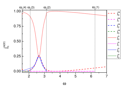
(a)

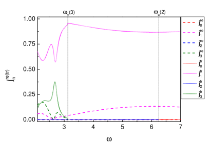
(b)

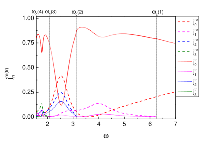
(c)

Figure 5: (Color online) The reflection/transmission coefficients $j_{n}$ via the potential strength $\omega$ with parameters (a) $m_{1}=1$, $K_{0}=5$, $\gamma_{1}=\gamma_{2}=1,l=0$; (b) $m_{1}=1$, $K_{0}=5$, $\gamma_{1}=\gamma_{2}=1,l=1$; (c) $m_{1}=1.1$, $K_{0}=5$, $\gamma_{1}=2,\gamma_{2}=1,l=0$.

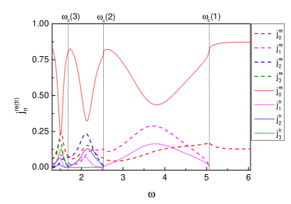
(a)

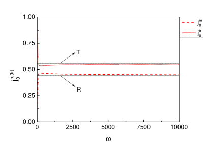
(b)

Figure 6: (Color online) The reflection/transmission coefficients $j_{n}$ via the coupling strength $\omega$ with parameters $m_{1}=1$, $K_{0}=4.5$, $\gamma_{1}=2$, $\gamma_{2}=0$, and (a) $\omega\in(1.3,6)$; (b) $\omega\in(6,10^{4})$. The black lines in (b) label the reflection and transmission coefficients for a single particle scattered by a delta-function potential (see text for details).

In our model, we assume a harmonic coupling as the binding potential, and the choice of $\omega$ determines how far the particles of the bound system can separate from each other. For a certain $K_{0}$, the critical coupling stiffness $\omega_{c}(n)$ to excite the $n$-th internal state is

$$\omega_{c}(n)=\frac{\hbar K_{0}^{2}}{2(n-l)M}.$$ (25)

when $\omega\leq\omega_{c}(n)$, the $n$-th mode may be excited. We exhibit the dependence of $j_{n}$ on the coupling stiffness $\omega$ in Fig. 5. Similar as discussed above, the scattering potential can only excite the modes whose parity are the same as that of incident mode for the symmetric Hamiltonian (Fig. 5a, Fig. 5b), while the other modes can also be excited for the asymmetric Hamiltonian (Fig. 5c). The greater influence of symmetric Hamiltonian on odd-parity modes still results in the characteristics ”peak” and ”valley” for $j_{3}^{re(tr)}$ in Fig. 5b.

We have discussed the situation where both particles interact individually with the scattering potential above, then we discuss the case $\gamma_{1}>0$ and $\gamma_{2}=0$ that corresponds to the situation where particle 2 is only affected indirectly by the scattering potential via the binding potential. Considering of two limiting cases, when the coupling stiffness is large enough, the internal degrees of freedom is confined in the ground state and the bound system reduces to a single particle, this problem is equivalent to that of a particle with mass $M$ scattered by a delta-function potential $\gamma\delta(X)$, the corresponding reflection and transmission coefficients are

$$R =\frac{\hbar^{4}K_{0}^{2}}{\hbar^{4}K_{0}^{2}+M^{2}\gamma^{2}},$$ (26)

$$T =\frac{M^{2}\gamma^{2}}{\hbar^{4}K_{0}^{2}+M^{2}\gamma^{2}}.$$ (27)

which are marked by the horizontal lines in Fig. 6b. As Fig. 6b indicates, the reflection and transmission coefficients $j_{0}^{re},j_{0}^{tr}$ converge to $R$ and $T$ respectively for the extreme large $\omega$.

As we mentioned above, particle 2 is affected by the potential via the binding potential, the proportion of particle 1 in the bound system will seriously affect the scattering process. In the limit $m_{1}\rightarrow 0$, i.e., $m_{1}/M\rightarrow 0$, this problem is equivalent to that of a particle with mass $M$ passing through the delta-function potential directly, namely, $j_{0}^{tr}=1,j_{0}^{re}=0$. On the other extreme, $m_{1}/M\rightarrow 1$, it reduces to the situation that one particle with $m_{1}$ is scattered by a delta-function potential, resulting in $j_{0}^{re}=R$ and $j_{0}^{tr}=T$ (see Fig. 7).

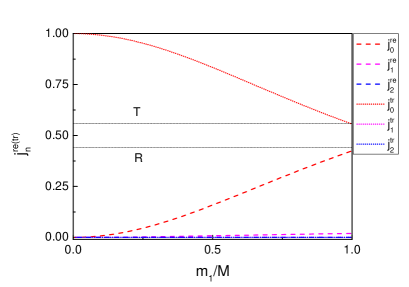
Figure 7: (Color online) The reflection/transmission coefficients $j_{n}$ via $m_{1}/M$ with parameters $K_{0}=4.5$, $\omega=2$, $\gamma_{1}=2$, $\gamma_{2}=0$. The black lines denote the reflection and transmission coefficients for a single particle scattered by a delta-function potential (see text for details).

(a)

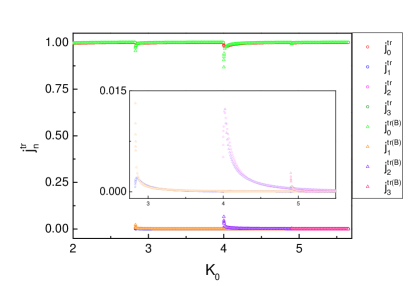
(b)

Figure 8: (Color online) The reflection coefficients $j_{n}^{re}$ (a) and transmission coefficients $j_{n}^{tr}$ (b) via the potential strength $\omega$ with parameters $m_{1}=1.1$, $\omega_{0}=2$, $\gamma_{1}=0.1,\gamma_{2}=0.05,l=0$, $j_{n}^{re/tr(B)}$are the analytical results within Born approximation.

In order to test the reliability and accuracy of our results, we derive the coefficients of reflection and transmission $j_{n}^{re},j_{n}^{tr}$ by using scattering matrix method within Born approximation, here $l$ is set to be $l=0$.

$$j_{0}^{re} = |\langle\phi_{-K_{0},0}|\mathcal{S}|\phi_{K_{0},0}\rangle|^{2}$$ (28)

$$\approx \frac{4\pi^{2}M^{2}}{K_{0}^{2}}|\langle\phi_{-K_{0},0}|V|\phi_{K_{0},0}\rangle|^{2},$$

$$j_{0}^{tr} =|\langle\phi_{K_{0},0}|\mathcal{S}|\phi_{K_{0},0}\rangle|^{2}$$

$$\approx 1+\frac{4\pi^{2}M^{2}}{K_{0}^{2}}|\langle\phi_{K_{0},0}|V|\phi_{K_{0},0}\rangle|^{2}$$

$$\quad{}+\frac{4\pi M}{K_{0}}\mathbf{Im}{\langle\phi_{K_{0},0}|VG_{0}^{+}V|\phi_{K_{0},0}\rangle}$$

$$=1+\frac{4\pi^{2}M^{2}}{K_{0}^{2}}|\langle\phi_{K_{0},0}|V|\phi_{K_{0},0}\rangle|^{2}-\frac{4\pi^{2}M^{2}}{K_{0}}\sum_{n=0}^{n_{c}}\frac{1}{K_{n}}$$

$$\quad{}\times\left(|\langle\phi_{-K_{n},n}|V|\phi_{K_{0},0}\rangle|^{2}+|\langle\phi_{K_{n},n}|V|\phi_{K_{0},0}\rangle|^{2}\right),$$ (29)

$$j_{n}^{re} = |\langle\phi_{-K_{n},n}|\mathcal{S}|\phi_{K_{0},0}\rangle|^{2}$$ (30)

$$\approx \frac{4\pi^{2}M^{2}}{K_{0}K_{n}}|\langle\phi_{-K_{n},n}|V|\phi_{K_{0},0}\rangle|^{2}$$

and

$$j_{n}^{tr} = |\langle\phi_{K_{n},n}|\mathcal{S}|\phi_{K_{0},0}\rangle|^{2}$$ (31)

$$\approx \frac{4\pi^{2}M^{2}}{K_{0}K_{n}}|\langle\phi_{K_{n},n}|V|\phi_{K_{0},0}\rangle|^{2}.$$

where $V=\gamma_{1}\delta(X-r_{2}x)+\gamma_{2}\delta(X+r_{1}x)$ and

$$\langle\phi_{\pm K_{n},n}|V|\phi_{K_{0},0}\rangle$$

$$=\frac{\gamma_{1}}{2\pi\sqrt{\mu\omega}}\mathbf{e}^{\frac{-(K_{n}-K_{0})^{2}r_{2}^{2}}{4\mu\omega}}\sqrt{\frac{2^{n}}{n!}}\left(\frac{i(K_{0}-K_{n})r_{2}}{2\sqrt{\mu\omega}}\right)^{n}$$

$$\quad{}+\frac{\gamma_{2}}{2\pi\sqrt{\mu\omega}}\mathbf{e}^{\frac{-(K_{n}-K_{0})^{2}r_{1}^{2}}{4\mu\omega}}\sqrt{\frac{2^{n}}{n!}}\left(\frac{i(K_{n}-K_{0})r_{1}}{2\sqrt{\mu\omega}}\right)^{n}.$$ (32)

It’s well known that Born approximate is no longer valid for a high barrier, in Fig. 8 we take $\gamma_{1}=0.1$, $\gamma_{2}=0.05$ and compare our numerical results with analytical ones. For $K_{0}$ away from $K_{0}^{c}(n)$, numerical simulations show qualitative agreement with these analytical results, while for $K_{0}\sim K_{0}^{c}(n)$, the analytical results are divergent, indicating the resonance between the incident mode with the to-be excited modes.

IV Discussion and summary

In summary, we have considered a diatomic bound system to simulate the composite system, and present how this system is scattered by a delta-function potential. This could be of importance for a scattering process of an actual composite system, and even for the testing of the quantum superposition with a macroscopic object, since we have considered the internal degrees of freedom. The wave function of the composite system can be splitted up into two components, leading to the realization of preparation of a spatial superposition.

When the incoming momentum of the center-of-mass degree of freedom is large enough, the scattering potential may excite internal states. We emphasize that the $n>n_{c}$ states could exist in the scattering region. Physically, these states decay when the system is far away from the scattering region since the outgoing momentums are imaginary, namely, there are only $n\leq n_{c}$ internal states being populated at infinite. Whether the $n\leq n_{c}$ internal states can be excited depends on both the symmetry of Hamiltonian and the energy condition. All the states under $n_{c}$ could be excited for an asymmetric Hamiltonian, whereas only the states whose parity are same as incident one could be excited for a symmetric Hamiltonian. The populations of internal modes are different for reflected and transmitted components, this should be taken into account in the experiments of composite system.

We find that the existence of internal degree of freedom can significantly change the reflection and transmission coefficients of the incident mode no matter whether the other modes are populated. And the symmetric Hamiltonian has a more serious impact on the odd-parity internal states than on the even-parity states.

Depending on the coupling strength between the two particles, and also on the mass of particle 1, the scattering of composite system can reduce to that of a single particle. Moreover, in the region where Born approximate is valid, simulation results are in a good accordance with those of analytical values.

In the present study, we employ a harmonic coupling to mimic the interaction between particles simply. Our further research within a general coupling potential, which can describe the process to transform a diatomic molecular to two atoms, is in process.

References

• (1) O. Romero-Isart, L. Clemente, C. Navau, A. Sanchez, and J. I. Cirac, Phys. Rev. Lett. 109, 147205 (2012).
• (2) A. Bassi, K. Lochan, S. Satin, T. P. Singh, H. Ulbricht, Rev. Mod. Phys. 85, 471 (2013).
• (3) W. Marshall, C. Simon, R. Penrose, and D. Bouwmeester, Phys. Rev. Lett. 91, 13 (2003).
• (4) O. Romero-Isart, M. L Juan, R. Quidant, and J. I. Cirac, New J. Phys. 12, 033015 (2010).
• (5) O. Romero-Isart, Phys. Rev. A 84, 052121 (2011).
• (6) T. Kovachy, P. Asenbaum, C. Overstreet, C. A. Donnelly, S. M. Dickerson, A. Sugarbaker, J. M. Hogan, and M. A. Kasevich, Nature 528, 530 (2015).
• (7) U. B. Hoff, J. Kollath-Bönig, J. S. Neergaard-Nielsen, and U. L. Andersen, Phys. Rev. Lett. 117, 143601 (2016).
• (8) J. Q. Liao, and L. Tian, Phys. Rev. Lett. 116, 163602 (2016).
• (9) M. Carlesso, A. Bassi, P. Falferi, and A. Vinante, Phys. Rev. D 94, 124036 (2016).
• (10) M. Abdi, P. Degenfeld-Schonburg, M. Sameti, C. Navarrete-Benlloch and M. J. Hartmann, Phys. Rev. Lett. 116, 233604 (2016).
• (11) W. Schöllkopf, and J. P. Toennies, Science 266, 1345 (1994).
• (12) M. Arndt, O. Nairz, J. Vos-Andreae, C. Keller, G. van der Zouw, and A. Zeilinger, Nature 401, 680 (1999).
• (13) S. Gerlich, S. Eibenberger, M. Tomandl, S. Nimmrichter, K. Hornberger, P. J. Fagan, J. Tüxen, M. Mayor, and M. Arndt, Nat. Commun. 2, 263 (2011).
• (14) L. L. Sánchez-Soto, J. J. Monzón, A. G. Barriuso, J. F. Cariñena, Phys. Rep. 513, 191 (2012).
• (15) A. Mostafazadeh, Phys. Rev. Lett. 102, 220402 (2009).
• (16) W. Trzeciakowski, M. Gurioli, J. Phys.: Condens. Matter 5, 1701 (1993).
• (17) L. V. Chebotarev, A. Tchebotareva, J. Phys. A: Math. Gen. 29, 7259 (1996).
• (18) M. G. Rozman, P. Reineker, R. Tehver, Phys. Lett. A 187, 127 (1994).
• (19) L. V. Chebotarev, Phys. Rev. A 52, 107 (1995).
• (20) F. Queisser, W. G. Unruh, Phys. Rev. D 94, 116018 (2016).
• (21) J. R. Taylor, Scattering Theory: The Quantum Theory on Nonrelativistic Collisions, Wiley, New York, 1972.
• (22) R. G. Newton, Scattering Theory of Waves and Particles, 2nd ed., Springer, New York, 1982.