An Explicit, Coupled-Layer Construction of a High-Rate Regenerating Code with Low Sub-Packetization Level, Small Field Size and $d<(n-1)$

Abstract

This paper presents an explicit construction for an $((n=2qt,k=2q(t-1),d=n-(q+1)),(\alpha=q(2q)^{t-1},\beta=\frac{\alpha}{q}))$ regenerating code (RGC) over a field $\mathbb{F}_{Q}$ having rate $\geq\frac{t-2}{t}$. The RGC code can be constructed to have rate $k/n$ as close to $1$ as desired, sub-packetization level $\alpha\leq r^{\frac{n}{r}}$ for $r=(n-k)$, field size $Q$ no larger than $n$ and where all code symbols can be repaired with the same minimum data download.

I Introduction

In an $((n,k,d),(\alpha,\beta))$ regenerating code [1] over the finite field $\mathbb{F}_{Q}$, a file of size $B$ over $\mathbb{F}_{Q}$ is encoded and stored across $n$ nodes in the network with each node storing $\alpha$ coded symbols. The parameter $\alpha$ is termed as the sub-packetization level of the code. A data collector can download the data by connecting to any $k$ nodes. In the event of node failure, node repair is accomplished by having the replacement node connect to any $d$ nodes and downloading $\beta\leq\alpha$ symbols from each node. The quantity $d\beta$ is termed the repair bandwidth. The focus here is on exact repair, meaning that at the end of the repair process, the contents of the replacement node are identical to that of the failed node.

It is well known that the file size $B$ must satisfy the upper bound (see [1]): $B\ \leq\ \sum_{\ell=1}^{k}\min\{\alpha,(d-\ell+1)\beta\}$. It follows from this that $B\leq k\alpha$ and equality is possible only if $\alpha\leq(d-k+1)\beta$.

I-A Literature on MSR Codes

A regenerating code is said to be a Minimum Storage Regenerating (MSR) code if $B=\alpha k$ and $\alpha=(d-k+1)\beta$, since the amount $n\alpha$ of data stored for given file size $B$ is then the minimum possible.

The definition of an MSR code requires that all nodes be repairable with the same minimum data download. There are papers however in the literature that refer to a code as being an MSR code even if the data download is a minimum only for the repair of systematic nodes. We will distinguish between the two classes by referring to them as all-node-repair and systematic-repair MSR codes respectively.

Several constructions of MSR codes can now be found in the literature. The product-matrix construction [2], provides MSR codes for any $2k-2\leq d\leq n-1$. In [3], high-rate MSR codes with parameters $(n,k=n-2,d=n-1)$ are constructed using Hadamard designs. In [4], high-rate systematic-repair MSR codes, known as zigzag codes, are constructed for $d=n-1$. This was subsequently extended to include the repair of parity nodes as well in [5]. In [6], Cadambe et al. show the existence of high-rate MSR codes for any value of $(n,k,d)$ as $\alpha$ scales to infinity.

Desirable attributes of an MSR code include an explicit construction, high-rate, low values of sub-packetization level $\alpha$ and small field size. While zigzag codes allow arbitrarily high rates to be achieved, a level of sub-packetization that is exponential in $k$ is required. In a subsequent paper [7], a systematic-repair MSR code having $\alpha=r^{\frac{k}{r+1}}$ is constructed. A lower bound $2\log_{2}\alpha(\log_{\left(\frac{r}{r-1}\right)}\alpha+1)+1\ \geq\ k$ on $\alpha$ is presented in [8]. A second lower bound on $\alpha$, $\alpha\geq r^{\frac{k}{r}}$, can be found in [9], that applies to a subclass of MSR codes known as help-by-transfer (also known in the literature as access-optimal) MSR codes. For help-by-transfer MSR codes, the number of symbols transmitted as helper data over the network is equal to the number of symbols accessed at the helper nodes. Prior to this in [10], the authors presented a construction of a systematic-repair MSR code that permits rates in the regime $\frac{2}{3}\leq R\leq 1$, and that has an $\alpha$ that is polynomial in $k$. In [11], explicit help-by-transfer systematic-repair MSR codes are presented with sub-packetization meeting the lower bound $\alpha\geq r^{\frac{k}{r}}$. However the constructions were limited for $r=2,3$. In [12], explicit help-by-transfer systematic-repair MSR codes are presented with sub-packetization meeting the lower bound $\alpha\geq r^{\frac{k}{r}}$ for any $k,r$. In [13], a high-rate MSR construction for $d=n-1$ is presented that has sub-packetization level $r^{\frac{n}{r}}$ and where all nodes are repaired with minimum data download. The construction provided was however, not explicit, and required large field size. This is extended for general $k\leq d\leq n-1$ in [14]. In [15], the authors provide a construction for a systematic-repair MSR code for all $k\leq d\leq n-1$, but these constructions are also non-explicit and require large field size. Though suboptimal in terms of repair bandwidth, a vector-MDS code supporting a family of $\alpha=r^{p},p\geq 1$ and efficient node-repair is presented in [16].

Most recently, in [17], Ye and Barg present an explicit construction of a high-rate MSR code having rate $k/n$ as close to $1$ as desired, sub-packetization level $\alpha=r^{\frac{n}{r}}$ for $r=(n-k)$, field size $Q$ no larger than $n$, $d=(n-1)$ and where all code symbols can be repaired with the same minimum data download. Essentially the same construction was rediscovered, albeit some two months later, by the authors of the present paper in [18]. The construction in [18] builds on the earlier construction in [13]. The authors of [16] observe that the construction in [17] can be extended for $d<n-1$ using the technique suggested in [14], resulting in a non-explicit construction. In [19], the authors present explicit MSR code constructions for $d<n-1$ that requires sub-packetization level $(d-k+1)^{n-1}$.

I-B Our Contribution

In the present paper, we show how the Coupled-Layer MSR code construction in [17] (or [18]) can be modified to handle the case when $d<(n-1)$ to yield an RGC having parameters:

$$(n=2qt,k=2q(t-1),d=n-(q+1)),$$

$$(\alpha=q(2q)^{t-1},\beta=\frac{\alpha}{q}),$$

over a field $\mathbb{F}_{Q}$ having rate $\geq\frac{t-2}{t}$. A smaller value of $d$ is appealing in practice because it provides greater flexibility in handling node repair. For instance, it allows one to avoid calling upon nodes that are either slow to respond or else, are otherwise occupied.

II Description of the RGC

II-A Code Parameters

Let $q\geq 2,t\geq 2$ be integers. Let ${\mathbb{Z}_{2q}}$ denote the set of integers modulo $2q$, $[t]$ denote the set $\{1,2,\cdots,t\}$ and $[0,2q-1]$ denote the set of integers $\{0,1,\cdots,2q-1\}$. We describe below the construction of an $\{(n,k,d),(\alpha,\beta)\}$ high-rate RGC over a finite field $\mathbb{F}_{Q}$ having parameters

$$\left(\ n=2qt,\ k=2q(t-1),\ d=n-(q+1)\ \right),$$

$$\left(\alpha=q\cdot(2q)^{t-1},\beta=(2q)^{t-1}\right)\text{ and }\ \ Q\leq n\ .$$

The file size $B$ of the RGC is such that the rate $R:=\frac{B}{n\alpha}$ of the RGC satisfies:

$$R \geq \frac{t-2}{t}.$$

The code is not however an MSR code as it does not meet the requirement $B=k\alpha$. We note that through shortening, we can obtain RGCs having $(n,k,d)=(n-\Delta_{s},k-\Delta_{s},d-\Delta_{s})$ for $0\leq\Delta_{s}\ \leq k-1$. Through puncturing, we can obtain RGCs having $(n,k,d)=(n-\Delta_{p},k,d)$ for $0\leq\Delta_{p}\leq n-d-1$. A few example parameters are given in the table below:

$(q,t),\Delta_{s}/\Delta_{p}$	Parameter set
	$n$	$k$	$d$	$\alpha$
$(2,3)$	12	8	9	32
$(2,3),\Delta_{p}=1$	11	8	9	32
$(2,3),\Delta_{s}=2$	10	6	7	32
$(2,4)$	16	12	13	128
$(3,4)$	24	16	20	648

II-B The Data Cube

The RGC constructed here can be described in terms of an array of symbols over $\mathbb{F}_{Q}$ as given below:

$${\cal A} = \left\{\mbox{$A(x,y;\underline{z})$}\mid x\in\mathbb{Z}_{2q},y\in[t],\underline{z}\in\mathbb{Z}_{2q}^{t}\right\}.$$

This array can be depicted as a data cube, see Fig. 1(a) of size $(2q\times t\times(2q)^{t})$.

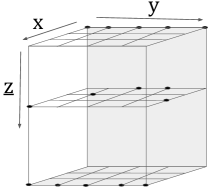
(a) The data cube containing $((2q\times t)\times(2q)^{t})$ symbols over the finite field $\mathbb{F}_{Q}$. In this example, $2q=4,t=5$.

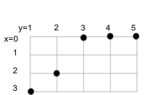
(b) We employ a dot notation to identify a plane. The example indicates the plane $\mbox{$\underline{z}$}\ =(3,2,0,0,0)$.

Figure 1: Illustration of the data cube.

In the figure, the cube appears as a collection of $(2q)^{t}$ planes, with each horizontal plane indexed by the parameter $\underline{z}$.

From the point of view of the RGC, the data cube corresponds to the data contained in a total of $n=2qt$ nodes, where each node is indexed by the pair of variables:

$$\left\{(x,y)\mid x\in\mathbb{Z}_{2q},y\in[t]\ \right\}.$$

The $(x,y)$th node stores the $\alpha_{0}=(2q)^{t}$ symbols

$$C(x,y) = \left\{\mbox{$A(x,y;\underline{z})$}\mid\underline{z}\in\mathbb{Z}_{2q}^{t}\right\}.$$ (1)

Thus each codeword in the RGC is made up of the $n=2qt$ vector code symbols $(C(x,y)\mid\mbox{$x\in\mathbb{Z}_{2q},y\in[t]$})$, in which each vector has $(2q)^{t}$ components indexed by $\underline{z}$. It will be explained in Sec. III-A how the $\alpha_{0}$ components in a vector are mapped to $\alpha$ symbols of a node in the RGC. Let $\Theta$ be a Vandermonde matrix that forms a parity-check matrix of an $[n,k]$-MDS code ${\cal J}$ . This can be constructed using field size $n$. We denote by $\theta^{\ell}_{(x,y)}$the entry of $\Theta$ at the location $(\ell,(x,y))$, $\ell\in[0,2q-1]$, $(x,y)\in\mathbb{Z}_{2q}\times[t]$ . Let $u\in\mbox{$\mathbb{F}_{Q}$}$ satisfy $u\neq 0,u^{2}\neq 1$.

By a slight abuse of notation, we will refer to the symbols $A(x,y;\underline{z})$ as code symbols (as opposed to calling them components of a code symbol) as most of our discussion will involve the symbols $A(x,y;\underline{z})$.

II-C Companion Terms, Transformed Code Symbols

Let us define

in other words, $\underline{z}_{(x,y)}$, is obtained by replacing the $y$th component of $\underline{z}$ by $x$. We next, set

$$A^{c}(x,y;\underline{z}) = \mbox{$A(z_{y},y;\underline{z}_{(x,y)})$},$$

and regard $\{\mbox{$A(x,y;\underline{z})$},\mbox{$A^{c}(x,y;\underline{z})$}\}$ as a set of paired elements and $A^{c}(x,y;\underline{z})$ as the companion of $A(x,y;\underline{z})$. Conversely, $A(x,y;\underline{z})$ is the companion of $A^{c}(x,y;\underline{z})$. Note however, that if $z_{y}=x$, then $\mbox{$A^{c}(x,y;\underline{z})$}=\mbox{$A(x,y;\underline{z})$}$ and the element $A(x,y;\underline{z})$ is paired with itself. For $\underline{z}$ such that $z_{y}\neq x$, we introduce the transformed code symbols  $B(x,y;\underline{z})$, $B^{c}(x,y;\underline{z})$:

$$\left[\begin{array}[]{c}\mbox{$B(x,y;\underline{z})$}\\ \mbox{$B^{c}(x,y;\underline{z})$}\end{array}\right] = \left[\begin{array}[]{cc}1&u\\ u&1\end{array}\right]\left[\begin{array}[]{c}\mbox{$A(x,y;\underline{z})$}\\ \mbox{$A^{c}(x,y;\underline{z})$}\end{array}\right],$$

where the inverse transformation is given by

$$\left[\begin{array}[]{c}\mbox{$A(x,y;\underline{z})$}\\ \mbox{$A^{c}(x,y;\underline{z})$}\end{array}\right] = \frac{1}{1-u^{2}}\left[\begin{array}[]{cc}1&-u\\ -u&1\end{array}\right]\left[\begin{array}[]{c}\mbox{$B(x,y;\underline{z})$}\\ \mbox{$B^{c}(x,y;\underline{z})$}\end{array}\right].$$

If however, $z_{y}=x$, we simply define

$$\mbox{$B(x,y;\underline{z})$}\ =\ \mbox{$B^{c}(x,y;\underline{z})$}\ =\ \mbox{$A(x,y;\underline{z})$}\ =\mbox{$A^{c}(x,y;\underline{z})$}.$$

It can be verified that all $4$ elements $\{\mbox{$B(x,y;\underline{z})$},\mbox{$B^{c}(x,y;\underline{z})$},\mbox{$A(x,y;\underline{z})$},\mbox{$A^{c}(x,y;\underline{z})$}\}$ can be determined from any $2$ of them.

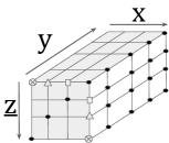
Figure 2: Illustrating $3$ sets of paired symbols $(\mbox{$A(x,y;\underline{z})$},\mbox{$A^{c}(x,y;\underline{z})$})$.

II-D Parity-Check Equations

The parity-check (p-c) equations required to be satisfied by the symbols $A(x,y;\underline{z})$ are of two types: $B$-plane p-c equations and nodal p-c equations.

The $B$-plane p-c equations are expressed in terms of the transformed code symbols $B(x,y;\underline{z})$ and are given by:

(5)

Thus there are in all, $(2q)\times(2q)^{t}$ $B$-plane p-c equations  with $2q$ equations indexed by the parameter $\ell$ per plane $\underline{z}$.

The nodal p-c equations involve only the symbols $A(x_{0},y_{0};\underline{z})$ lying within the same node. For fixed $(x_{0},y_{0})\in\mathbb{Z}_{2q}\times[t]$, there are a total of $\left(q\times(2q)^{t-1}\right)$ equations of the form

(6)

obtained by varying $\ell$, over $0\leq\ell\leq(q-1)$ and varying $z_{i},1\leq i\leq t,i\neq y_{0}$ over all of $\mathbb{Z}_{2q}$, with $z_{y_{0}}=x_{0}$ fixed. These can be alternately be described in terms of their companions as given below:

(7)

where the $\left(q\times(2q)^{t-1}\right)$ equations are obtained this time, by varying $\ell$, over $0\leq\ell\leq(q-1)$ and varying $\mbox{$\underline{z}$}\in\mathbb{Z}_{2q}^{t}$ while maintaining $z_{y_{0}}=x_{0}$.

III Parameters of the Proposed RGC

In the sections to follow, it will be shown that the code constructed above, yields an RGC having parameters

and having rate $\geq\frac{t-2}{t}$.

III-A The Value of $\alpha$

With respect to the data cube $\{A(x,y;\mbox{$\underline{z}$})\mid\mbox{$x\in\mathbb{Z}_{2q},y\in[t]$},\mbox{$\underline{z}$}\in\mbox{$\mathbb{Z}_{2q}$}^{t}\}$, each pair $(x,y)$ identifies a distinct node. At the outset each node appears to contain $(2q)^{t}$ symbols leading to $\alpha=(2q)^{t}$. However, these symbols are not linearly independent, since they are subject to the nodal parity-check equations (6). For a given node $(x_{0},y_{0})$, there are a total of $(2q)^{t}/2$ parity-check equations corresponding to a parity-check matrix $J$ having a block-diagonal form:

$$\underbrace{J_{0}}_{(\ (2q)^{t}/2\ \times\ (2q)^{t}\ )} = \left[\begin{array}[]{cccc}\underbrace{J}_{(q\times 2q)}&&&\\ &J_{0}&&\\ &&\ddots&\\ &&&J_{0}\end{array}\right]$$

Each of the matrices $J_{0}$ is a Vandermonde matrix, hence $J$ has full rank, which means that each node contains just $(2q)^{t}/2$ linearly independent symbols. We can thus set $\alpha=(2q)^{t}/2$.

III-B File Size and Rate of the RGC

The total number of parity-check equations, including both $B$-plane p-c equations and nodal p-c equations, is given by:

$$\underbrace{2qt(2q)^{t-1}q}_{\text{nodal}}+\underbrace{(2q)^{t}2q}_{\text{planar}}\ =\ (2q)^{t}(qt+2q).$$

As $\alpha_{0}$ denotes the number of symbols per node without considering linear dependence among them, we have

$$n\alpha_{0} = (2qt)(2q)^{t}.$$

It follows that the file size $B$ satisfies the lower bound:

$$B \geq n\alpha_{0}\ -\ (2q)^{t}(qt+2q)$$

$$= (2qt)(2q)^{t}\ -\ (2q)^{t}(qt+2q)$$

$$= (2q)^{t}\left\{q(t-2)\right\}.$$

This leads to the rate bound

$$R \geq \frac{t-2}{t}.$$

We note that an MSR code having the same parameters would have rate $\frac{k}{n}\ =\ \frac{t-1}{t}$.

IV Pictorial Representation for Planes that Identifies Erased Nodes

We associate with each plane $\underline{z}$, a $(2q\times t)$ $\{0,1\}$ incidence matrix $P(\underline{z})$ given by

$$P_{(x,y)}(\underline{z}) = \left\{\begin{array}[]{rl}1&z_{y}=x\\ 0&\text{else}.\end{array}\right.$$

Let ${\cal E}=\{(x_{i},y_{i})\in\mathbb{Z}_{2q}\times[t]\mid 1\leq i\leq 2q\}$ denote the location of the $2q$ erased nodes. Given an erasure pattern ${\cal E}$  and a plane $\underline{z}$  we define a $(2q\times t)$ $\{0,1\}$ incidence matrix $P(\mbox{${\cal E}$},\underline{z})$ which is the matrix $P(\underline{z})$ with the entries corresponds to the erased nodes circled. For example, if $\mbox{${\cal E}$}\ \ =\ \{(0,2),(1,2),(2,2),(2,4)\}$, with $\mbox{$\underline{z}$}=[1\ 2\ 3\ 1\ 0]^{t}$, we obtain:

$$P({\cal E},\underline{z})\ =\ \left[\begin{array}[]{ccccc}0&\leavevmode\hbox to14.18pt{\vbox to14.18pt{\text{[drawing]}}}&0&0&1\\ 1&\leavevmode\hbox to14.18pt{\vbox to14.18pt{\text{[drawing]}}}&0&1&0\\ 0&\leavevmode\hbox to14.18pt{\vbox to14.18pt{\text{[drawing]}}}&0&\leavevmode\hbox to14.18pt{\vbox to14.18pt{\text{[drawing]}}}&0\\ 0&0&1&0&0\end{array}\right].$$

IV-A Intersection Score of an Erasure Pattern on a Plane

Given a plane $\underline{z}$ $\in\mathbb{Z}_{2q}^{t}$ and an erasure pattern ${\cal E}$, we define the intersection score $\sigma\mbox{$({\cal E},\mbox{$\underline{z}$})$}$ to be given by

$$\sigma\mbox{$({\cal E},\mbox{$\underline{z}$})$} = \mid\left\{y\in[t]\mid(z_{y},y)\in\mbox{${\cal E}$}\right\}\mid,$$ (11)

and set $\sigma_{\max}(\mbox{${\cal E}$})=\max\{\sigma(\mbox{${\cal E}$},\mbox{$\underline{z}$})\mid\mbox{$\underline{z}$}\in\mathbb{Z}_{2q}^{t}\}$. In terms of the matrix $P({\cal E},\underline{z})$, the intersection score equals the number of circled entries that equal $1$, and hence $\sigma\mbox{$({\cal E},\mbox{$\underline{z}$})$}=1$ in the example above.

V Sequential Decoding Approach to Data Collection

The data collection property requires that we can recover the data in the presence of $(n-k)=2q$ erasures. Let $\mbox{${\cal E}$}=\{(x_{i},y_{i})\mid 1\leq i\leq 2q\}$ be a fixed erasure pattern. First, we make use of the nodal equations to recover $\alpha$ symbols in each of the $k$ surviving nodes. Then the aim is to recover the erased code symbols, $\{A(x_{i},y_{i};\underline{z})\mid 1\leq i\leq[t],\mbox{$\underline{z}$}\ \in\mathbb{Z}_{2q}^{t}\}$. We adopt a sequential procedure in which the erased symbols are decoded successively in increasing order of intersection score $s$, $0\leq s\leq\sigma_{\max}(\mbox{${\cal E}$})$. The decoding algorithm that relies upon only the $B$-plane p-c equations remains the same as the one described in [18].

V-A Case of Zero Intersection Score

Let $\underline{z}$ be a fixed plane having intersection score zero. The $2q$ $B$-plane p-c equations associated to $\underline{z}$ are given by

$$\sum\limits_{\mbox{$x\in\mathbb{Z}_{2q},y\in[t]$}}\left\{A(x,y;\mbox{$\underline{z}$})+uA^{c}(x,y;\mbox{$\underline{z}$})\right\}\theta_{(x,y)}^{\ell} = 0.$$

Since $\mbox{$\underline{\sigma}({\cal E},\underline{z})$}=0$, we have that $(z_{y},y)\not\in{\cal E},\text{for any }y\in[t]$. As a result, the companion symbol $A^{c}(x,y;\underline{z})$ which lies in node $(z_{y},y)$, is not erased. It follows that for symbols $A(x,y;\underline{z})$ with $(x,y)\not\in{\cal E}$, both $A(x,y;\underline{z})$ and $A^{c}(x,y;\underline{z})$ are known. The same argument tells us that for symbols $A(x,y;\underline{z})$ with $(x,y)\in{\cal E}$, while $A(x,y;\underline{z})$ is unknown, $A^{c}(x,y;\underline{z})$ is known. Hence, we can rewrite the parity-check equations associated to plane $\underline{z}$ equations in the form $\sum\limits_{(x,y)\in\mbox{${\cal E}$}}A(x,y;\mbox{$\underline{z}$})\ \theta_{(x,y)}^{\ell}\ =\ \kappa_{*}$, where $\kappa_{*}$ is generic notion for a known element in the finite field $\mathbb{F}_{Q}$ that can be determined from the non-erased code symbols. We are thus left with a set of $2q$ equations involving $2q$ unknowns and a Vandermonde coefficient matrix, so the symbols $A(x,y;\mbox{$\underline{z}$})$ lying in a place $\underline{z}$ having intersection-score zero can in this way, be recovered.

V-B Case of Intersection Score $\sigma>0$

We show here how one can inductively recover code symbols corresponding to planes $\underline{z}$ having intersection score $\mbox{$\underline{\sigma}({\cal E},\underline{z})$}>0$, given that symbols in planes $\mbox{$\underline{z}$}^{\prime}$ with $\sigma({\cal E},\mbox{$\underline{z}$}^{\prime})<\mbox{$\underline{\sigma}({\cal E},\underline{z})$}$ have already been recovered.

Let an erasure pattern ${\cal E}$ and a plane $\underline{z}$ be fixed. We first partition the $2q$-erasure location set ${\cal E}$ into disjoint subsets,

$$\mbox{${\cal E}$}_{0,\underline{z}} = \left\{(x,y)\in\mbox{${\cal E}$}\mid x=z_{y}\right\},$$

$$\mbox{${\cal E}$}_{1,\underline{z}} = \left\{(x,y)\in\mbox{${\cal E}$}\mid(z_{y},y)\notin\mbox{${\cal E}$}\text{ hence $x\neq z_{y}$}\right\},$$

$$\mbox{${\cal E}$}_{2,\underline{z}} = \left\{(x,y)\in\mbox{${\cal E}$}\mid(z_{y},y)\in\mbox{${\cal E}$},\ x\neq z_{y}\right\}.$$

It can be verified that in the case of a symbol $A(x,y;\underline{z})$ with $(x,y)\not\in{\cal E}$, the companion symbol $A^{c}(x,y;\underline{z})$ lies either in an unerased node or else in a plane having a lower intersection score, and thus has already been recovered. For this reason, we can assume that the symbols $B(x,y;\underline{z})$ with $(x,y)\not\in{\cal E}$ are known and the parity-check equations in the inductive decoding process, can once again, be restricted to the erased symbols and their companions, i.e., can be assumed to be of the form

$$\sum\limits_{(x,y)\in\mbox{${\cal E}$}}\mbox{$B(x,y;\underline{z})$}\ \ \theta_{(x,y)}^{\ell} = \kappa_{*}.$$

These equations allow us to determine the value of the transformed code symbols $\{\mbox{$B(x,y;\underline{z})$}\ \mid(x,y)\in{\cal E}\}$.

• In the case of symbols $\{\mbox{$B(x,y;\underline{z})$}\ \mid(x,y)\in\mbox{${\cal E}$}_{0,\underline{z}}\}$, we have $\mbox{$A(x,y;\underline{z})$}=\mbox{$B(x,y;\underline{z})$}$ and thus we have recovered the symbols $A(x,y;\underline{z})$ in this instance.

• In the case of the symbols $\{\mbox{$B(x,y;\underline{z})$}\ \mid(x,y)\in\mbox{${\cal E}$}_{1,\underline{z}}\}$, we have that the complement $A^{c}(x,y;\underline{z})$ does not belong to an erased node and is hence known. From $B(x,y;\underline{z})$ and $A^{c}(x,y;\underline{z})$ one can recover $A(x,y;\underline{z})$, and so we are done even in this case.

• This leaves us only with having to recover symbols $\{\mbox{$A(x,y;\underline{z})$}\ \mid(x,y)\in\mbox{${\cal E}$}_{2,\underline{z}}\}$. In the case of such symbols, the companion $A^{c}(x,y;\underline{z})$ can be verified to also belong to a plane having the same intersection score as $\underline{z}$ and hence we can assume that both $B(x,y;\underline{z})$ and $B^{c}(x,y;\underline{z})$ have been determined. From these values, one can determine the value of $A(x,y;\underline{z})$.

This concludes the decoding process.

VI Node Repair

We turn in this section to node repair and assume node $(x_{1},y_{1})$ to be the failed node. Since there are a total of $d=n-q-1$ helper nodes, there are a set of $q$ nodes which do not participate in the repair process and which we will term as aloof nodes. Nodes that are not aloof and which do not correspond to the failed node, will be termed as helper nodes.

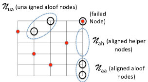
Figure 3: Illustrating the partioning of ${\cal E}$ into aligned (${\cal N}_{aa}$) and unaligned aloof nodes (${\cal N}_{an}$) and aligned helper nodes (${\cal N}_{ah})$.

VI-A Aligned and Unaligned Nodes

We will declare that two nodes to be aligned if their $y$ coordinates are the same. Let $\left\{(x_{i},y_{i})\ |\ 2\leq i\leq(q+m)\right\}$ denote the coordinates of the helper nodes aligned with $(x_{1},y_{1})$. Let us assume that of the $q$ aloof nodes, $(q-m)$ aloof nodes, namely, $\left\{(x_{i},y_{i})\ |\ q+m+1\leq i\leq 2q\right\}$, are aligned with the failed node and $m$ of them, namely, $\left\{(x_{i},y_{i})\ |\ 2q+1\leq i\leq 2q+m\right\}$, are not aligned. We set:

$${\cal N}=(x_{1},y_{1})\cup{\cal N}_{ah}\cup{\cal N}_{aa}\cup{\cal N}_{ua}.\hskip 72.26999pt$$

VI-B The Starting Equations

During the repair process, the aloof nodes and the single failed node together behave as though they together constitute a set of $(q+1)$ erased nodes. For this reason, we set

$${\cal E} = \{(x_{1},y_{1})\}\cup\mbox{${\cal N}_{aa}$}\cup\mbox{${\cal N}_{ua}$},$$

and retain the notation $\underline{\sigma}({\cal E},\underline{z})$ with regard to intersection score.

While each node $(x,y)$ only stores $\alpha$ non-redundant symbols, it nevertheless has access through computation, to all $(2q)^{t}$ symbols $\{\mbox{$A(x,y;\underline{z})$},\mbox{$\underline{z}$}\ \in\mbox{$\mathbb{Z}_{2q}^{t}$}\}$. Therefore the code does not support help-by-transfer repair. But the only computation required at any helper node is decoding of a half-rate RS code. During the repair of node $(x_{1},y_{1})$, we will only call upon the $\beta=(2q)^{t-1}$ symbols $\{\mbox{$A(x,y;\underline{z})$}\mid z_{y_{1}}=x_{1}\}$ from a helper node $(x,y)$.

VI-B1 Planes with intersection score $1$

Consider first, planes $\underline{z}$ which are such that $z_{y_{1}}=x_{1}$ and $z_{y_{i}}\neq x_{i}$ for any aloof node. Such planes have intersection score $\mbox{$\underline{\sigma}({\cal E},\underline{z})$}=1$. The $B$-plane p-c equations in such a plane take on the form:

$$\sum_{\mbox{$x\in\mathbb{Z}_{2q},y\in[t]$}}\mbox{$B(x,y;\underline{z})$}\ \mbox{$\theta^{\ell}_{(x,y)}$} = 0.$$ (12)

It can be verified that for $(x,y)\not\in{\cal N}$, the symbols $A(x,y;\underline{z})$ and $A^{c}(x,y;\underline{z})$ are both available for node repair and from these two values, one can compute $B(x,y;\underline{z})$. Hence we can rewrite (12) in the form:

$$\sum_{(x,y)\in\mbox{${\cal N}$}}\mbox{$B(x,y;\underline{z})$}\ \mbox{$\theta^{\ell}_{(x,y)}$} = \mbox{$\kappa_{*}$}.$$ (13)

For brevity in writing we set:

$$a_{i}\ =\ A(x_{i},y_{i};\mbox{$\underline{z}$}), a^{c}_{i}\ =\ A^{c}(x_{i},y_{i};\mbox{$\underline{z}$}),$$

$$b_{i}\ =\ B(x_{i},y_{i};\mbox{$\underline{z}$}), b^{c}_{i}\ =\ B^{c}(x_{i},y_{i};\mbox{$\underline{z}$}),$$

$$\theta_{i}\ =\ \theta_{(x_{i},y_{i})}, \underline{a}^{c}_{ah}\ =\ [a_{2}^{c},\cdots,a_{q+m}^{c}]^{T},$$

$$\underline{b}_{aa}\ =\ [b_{q+m+1},\cdots,b_{2q}]^{T}, \underline{b}_{ua}\ =\ [b_{2q+1},\cdots,b_{2q+m}]^{T}.$$

We have the following situation:

Node in ${\cal N}_{ah}$	$a_{i}$ known, $a_{i}^{c}$ always unknown
Node in ${\cal N}_{aa}$	$a_{i}$ unavailable, $a_{i}^{c}$ always unknown
Node in ${\cal N}_{ua}$	$a_{i}$ unavailable, $a_{i}^{c}$ can be unknown

The allows us to rewrite (13) in the form:

$$\left[\begin{array}[]{ccc}1&\cdots&1\\ \theta_{1}&\cdots&\theta_{2q+m}\\ \vdots&\vdots&\vdots\\ \theta_{1}^{2q-1}&\cdots&\theta_{2q+m}^{2q-1}\\ \end{array}\right]\left[\begin{array}[]{c}a_{1}^{c}\\ u\underline{a}^{c}_{ah}\\ \underline{b}_{aa}\\ \underline{b}_{ua}\end{array}\right] = \kappa_{*}.$$ (22)

Apart from these $2q$ plane-parity equations , we also have the $q$ nodal parity-equations associated to node $(x_{1},y_{1})$:

$$\left[\begin{array}[]{ccc}1&\cdots&1\\ \theta_{1}&\cdots&\theta_{2q}\\ \vdots&\vdots&\vdots\\ \theta_{1}^{q-1}&\cdots&\theta_{2q}^{q-1}\\ \end{array}\right]\left[\begin{array}[]{c}a_{1}^{c}\\ ua_{2}^{c}\\ \vdots\\ ua_{2q}^{c}\\ \end{array}\right] = \kappa_{*}.$$ (31)

Through row-reduction of the parity-check matrix, we can rewrite (31) in the form:

$$\leavevmode\resizebox{422.77661pt}{}{$\left[\begin{array}[]{c|c|c}\underbrace{C_{1}}_{(m\times q)}&I_{m}&\underbrace{[0]}_{(m\times(q-m))}\\ \hline\cr\underbrace{C_{2}}_{(q-m\times q)}&\underbrace{[0]}_{((q-m)\times m)}&I_{q-m}\\ \end{array}\right]\left[\begin{array}[]{c}a_{1}^{c}\\ ua_{2}^{c}\\ \vdots\\ ua_{2q}^{c}\\ \end{array}\right]\ =\ \kappa_{*}$}.$$ (38)

Combining (22) and first $m$ equations in (38) along with further row-reduction, we obtain: (see [21] for details)

$$\leavevmode\resizebox{422.77661pt}{}{$\left[\begin{array}[]{c|c|c|c}\underbrace{[0]}_{(m\times q)}&\underbrace{[0]}_{(m\times m)}&\underbrace{[0]}_{(m\times(q-m))}&\underbrace{C_{3}}_{(m\times m)}\\ \hline\cr\lx@intercol\hfil\underbrace{V\left(\{\theta_{i}^{j}\}^{2q-1}_{j=0},\ i\in[2q]\right)}_{((2q)\times(2q))}\hfil\lx@intercol\vrule\lx@intercol&\underbrace{[0]}_{(2q\times m)}\end{array}\right]\left[\begin{array}[]{c}a_{1}^{c}\\ u\underline{a}^{c}_{ah}\\ \underline{b}_{aa}\\ \underline{b}_{ua}\end{array}\right]\ =\ \kappa_{*}$}.$$ (45)

Clearly, the matrix on the left is nonsingular since $C_{3}$ is a Cauchy matrix and it follows therefore that we can recover the unknown vector: $[a_{1}^{c},\ u[\underline{a}^{c}_{ah}]^{T},\ [\underline{b}_{aa}]^{T},\ [\underline{b}_{ua}]^{T}]^{T}$. The vector $[a_{1}^{c},\ [\underline{a}^{c}_{ah}]^{T}]^{T}$ consists of $(q+m)$ symbols from the same node that participate in the $q$ nodal p-c equations involving $2q$ symbols. Thus we can decode $2q$ symbols $\{A(x_{1},y_{1};\underline{z}_{(x,y_{1})}\mid x\in\mathbb{Z}_{2q}\}$ belonging to the failed node.

The case of planes having intersection score $>1$ can be shown to reduce to the case of plane shaving intersection score $1$ using arguments similar to those employed in describing how data collection is carried out. For lack of space, we omit the details.

References

• [1] A. Dimakis, P. Godfrey, Y. Wu, M. Wainwright, and K. Ramchandran, “Network coding for distributed storage systems,” IEEE Trans. Inf. Theory, vol. 56, no. 9, pp. 4539–4551, Sep. 2010.
• [2] K. V. Rashmi, N. B. Shah, and P. V. Kumar, “Optimal Exact-Regenerating Codes for Distributed Storage at the MSR and MBR Points via a Product-Matrix Construction,” IEEE Trans. Inf. Theory, vol. 57, no. 8, pp. 5227–5239, Aug. 2011.
• [3] D. Papailiopoulos, A. Dimakis, and V. Cadambe, “Repair Optimal Erasure Codes through Hadamard Designs,” IEEE Trans. Inf. Theory, vol. 59, no. 5, pp. 3021–3037, 2013.
• [4] I. Tamo, Z. Wang, and J. Bruck, “Zigzag codes: MDS array codes with optimal rebuilding,” IEEE Trans. Inf. Theory, vol. 59, no. 3, pp. 1597–1616, 2013.
• [5] Wang, Z. and Tamo, I. and Bruck, J., “On Codes for Optimal Rebuilding Access,” in Proc. IEEE 47th Annual Allerton Conference on Communication, Control, and Computing, 2009, pp. 1374–1381.
• [6] V. Cadambe, S. A. Jafar, H. Maleki, K. Ramchandran, and C. Suh, “Asymptotic interference alignment for optimal repair of mds codes in distributed storage,” IEEE Trans. Inf. Theory, vol. 59, no. 5, pp. 2974–2987, 2013.
• [7] Z. Wang, I. Tamo, and J. Bruck, “Long MDS codes for optimal repair bandwidth,” in Proc. IEEE International Symposium on Information Theory, ISIT, 2012, pp. 1182–1186.
• [8] S. Goparaju, I. Tamo, and A. R. Calderbank, “An improved sub-packetization bound for minimum storage regenerating codes,” IEEE Trans. on Inf. Theory, vol. 60, no. 5, pp. 2770–2779, 2014.
• [9] I. Tamo, Z. Wang, and J. Bruck, “Access versus bandwidth in codes for storage,” IEEE Trans. Information Theory, vol. 60, no. 4, pp. 2028–2037, 2014.
• [10] V. R. Cadambe, C. Huang, J. Li, and S. Mehrotra, “Polynomial length MDS codes with optimal repair in distributed storage,” in Conference Record of the Forty Fifth Asilomar Conference on Signals, Systems and Computers ACSCC, 2011, pp. 1850–1854.
• [11] N. Raviv, N. Silberstein, and T. Etzion, “Access-optimal MSR codes with optimal sub-packetization over small fields,” CoRR, vol. 1505.00919, 2015.
• [12] G. K. Agarwal, B. Sasidharan, and P. V. Kumar, “An alternate construction of an access-optimal regenerating code with optimal sub-packetization level,” in National Conference on Communication (NCC), 2015.
• [13] B. Sasidharan, G. K. Agarwal, and P. V. Kumar, “A high-rate MSR code with polynomial sub-packetization level,” in Proc. IEEE International Symposium on Information Theory, ISIT, 2015, pp. 2051–2055.
• [14] A. S. Rawat, O. O. Koyluoglu, and S. Vishwanath, “Progress on high-rate MSR codes: Enabling arbitrary number of helper nodes,” CoRR, vol. 1601.06362, 2016.
• [15] S. Goparaju, A. Fazeli, and A. Vardy, “Minimum storage regenerating codes for all parameters,” CoRR, vol. 1602.04496, 2016.
• [16] V. Guruswami and A. S. Rawat, “New MDS codes with small sub-packetization and near-optimal repair bandwidth,” CoRR, vol. abs/1608.00191, 2016.
• [17] M. Ye and A. Barg, “Explicit constructions of optimal-access MDS codes with nearly optimal sub-packetization,” CoRR, vol. abs/1605.08630, 2016.
• [18] B. Sasidharan, M. Vajha, and P. V. Kumar, “An explicit, coupled-layer construction of a high-rate MSR code with low sub-packetization level, small field size and all-node repair,” CoRR, vol. abs/1607.07335, 2016.
• [19] M. Ye and A. Barg, “Explicit constructions of high-rate MDS array codes with optimal repair bandwidth,” CoRR, vol. 1604.00454, 2016.
• [20] B. Sasidharan, M. Vajha, and P. V. Kumar, “An explicit, coupled-layer construction of a high-rate msr code with low sub-packetization level, small field size and $d<(n-1)$,” in 2017 IEEE International Symposium on Information Theory (ISIT), 2017, pp. 2048–2052.
• [21] ——, “An explicit, coupled-layer construction of a high-rate regenerating code with low sub-packetization level, small field size and $d<(n-1)$,” CoRR, vol. abs/1701.07447v1, 2017.