Non-colocated Time-Reversal MUSIC: High-SNR Distribution of Null Spectrum

Abstract

We derive the asymptotic distribution of the null spectrum of the well-known Multiple Signal Classification (MUSIC) in its computational Time-Reversal (TR) form. The result pertains to a single-frequency non-colocated multistatic scenario and several TR-MUSIC variants are here investigated. The analysis builds upon the 1st-order perturbation of the singular value decomposition and allows a simple characterization of null-spectrum moments (up to the 2nd order). This enables a comparison in terms of spectrums stability. Finally, a numerical analysis is provided to confirm the theoretical findings.

I Introduction

Time-Reversal (TR) refers to all those methods which exploit the invariance of the wave equation (in lossless and stationary media) by re-transmitting a time-reversed version of the scattered (or radiated) field measured by an array to focus on a scattering object (or radiating source), by physical [1] or synthetic [2] means. In the latter case (computational TR), it consists in numerically back-propagating the field data by using a known Green’s function, representative of the propagation medium. Since the employed Green function depends on the object (or source) position, an image is formed by varying the probed location (this procedure is referred to as “imaging”). Computational TR has been successfully applied in different contexts such as subsurface prospecting [3], through-the-wall [4] and microwave imaging [5].

The key entity in TR-imaging is the Multistatic Data Matrix (MDM), whose entries are the scattered field due to each Transmit-Receive (Tx-Rx) pair. Two popular methods for TR-imaging are the decomposition of TR operator (DORT) [6] and the TR Multiple Signal Classification (TR-MUSIC) [7]. DORT imaging exploits the MDM spectrum by back-propagating each eigenvector of the so-called signal subspace, thus allowing to selectively focus on each (well-resolved) scatterer. On the other hand, TR-MUSIC imaging is based on a complementary point of view and relies on the noise subspace (viz. orthogonal-subspace), leading to satisfactory performance as long as the data space dimension exceeds the signal subspace dimension and sufficiently high Signal-to-Noise-Ratio (SNR) is present. TR-MUSIC was first introduced for a Born Approximated (BA) linear scattering model [7] and, later, successfully applied to the Foldy-Lax (FL) non-linear model [8]. Also, it became popular mainly due to: ($a$) algorithmic efficiency; ($b$) no need for approximate scattering models; and ($c$) finer resolution than the diffraction limits (especially in scenarios with few scatterers). Recently, TR-MUSIC has been expanded to extended scatterers in [9].

Though a vast literature on performance analysis of MUSIC [10] for Direction-Of-Arrival (DOA) estimation exists (see [11, 12] for resolution studies and [13, 14, 15, 16] for asymptotic Mean Squared Error (MSE) derivation, with more advanced studies presented in [17, 18, 19]), such results cannot be directly applied to TR-MUSIC. Indeed, in TR framework scatterers/sources are generally assumed deterministic and more importantly a single snapshot is used, whereas MUSIC results for DOA refer to a different asymptotic condition (i.e. a large number of snapshots). Also, to our knowledge, no corresponding theoretical results have been proposed in the literature for TR-MUSIC, except for [20, 21], providing the asymptotic (high-SNR) localization MSE for point-like scatterers. Yet, a few works have tackled achievable theoretical performance both for BA and FL models via the Cramér-Rao lower-bound [22].

In this letter we provide a null-spectrum analysis of TR-MUSIC for point-like scatterers, via a 1st-order perturbation of Singular Value Decomposition (SVD) [24], thus having asymptotic validity (i.e. meaning a high SNR regime). The present results are based on a homogeneous background assumption and neglecting mutual coupling, as well as polarization or antenna pattern effects. Here we build upon [25] (tackling the simpler colocated case) and consider a general non-colocated multistatic setup with BA/FL models where several TR-MUSIC variants, proposed in the literature, are here investigated. The obtained results complement those found in DOA literature [23] and allow to obtain both the mean and the variance of each null-spectrum, as well as to draw-out its pdf. Also, they highlight performance dependence of null-spectrum on the scatterers/arrays configurations and compare TR-MUSIC variants in terms of spectrum stability. We recall that stability property is important for TR-MUSIC, and has been investigated by numerical means [26, 27] or using compressed-sensing based approaches [28]. Finally, a few numerical examples, for a 2-D geometry with scalar scattering, are presented to confirm our findings.

The letter is organized as follows: Sec. II describes the system model and reviews classic results on SVD perturbation analysis. Sec. III presents the theoretical characterization of TR-MUSIC null-spectrum, whereas its validation is shown in Sec. IV via simulations. Finally, conclusions are in Sec. V.

II System Model

We consider localization of $M$ point-like scatterers at unknown positions $\{\bm{x}_{k}\}_{k=1}^{M}$ in $\mathbb{R}^{p}$ with unknown scattering potentials $\{\tau_{k}\}_{k=1}^{M}$ in $\mathbb{C}$. The Tx (resp. Rx) array consists of $N_{T}$ (resp. $N_{R}$) isotropic point elements (resp. receivers) located at $\{\tilde{\bm{r}}_{i}\}_{i=1}^{N_{T}}$ in $\mathbb{R}^{p}$ (resp. $\{\bar{\bm{r}}_{j}\}_{j=1}^{N_{R}}$ in $\mathbb{R}^{p}$). The illuminators first send signals to the probed scenario (in a known homogeneous background with wavenumber $\kappa$) and the transducer array records the received signals. The (single-frequency) measurement model is then [30]:

$$\bm{K}_{n} = \bm{K}(\bm{x}_{1:M},\bm{\tau})+\bm{W}$$ (1)

$$= \bm{G}_{\mathrm{r}}(\bm{x}_{1:M})\,\bm{M}(\bm{x}_{1:M},\bm{\tau})\,\bm{G}_{\mathrm{t}}(\bm{x}_{1:M})^{T}+\bm{W}$$ (2)

where $\bm{K}_{n}\in\mathbb{C}^{N_{R}\times N_{T}}$ (resp. $\bm{K}(\bm{x}_{1:M},\bm{\tau})$) denotes the measured (resp. noise-free) MDM. Differently $\bm{W}\in\mathbb{C}^{N_{R}\times N_{T}}$ is a noise matrix s.t. $\mathrm{vec}(\bm{W})\sim\mathcal{N}_{\mathbb{C}}(\bm{0}_{N},\sigma_{w}^{2}\,\bm{I}_{N})$, where $N\triangleq N_{T}N_{R}$. Additionally, we have denoted: ($i$) the vector of scattering coefficients as $\bm{\tau}\triangleq\left[\begin{array}[]{ccc}\tau_{1}&\cdots&\tau_{M}\end{array}\right]^{T}\in\mathbb{C}^{M\times 1}$; ($ii$) ($b$) the Tx (resp. Rx) array matrix as $\bm{G}_{\mathrm{t}}(\bm{x}_{1:M})\in\mathbb{C}^{N_{T}\times M}$ (resp. $\bm{G}_{\mathrm{r}}(\bm{x}_{1:M})\in\mathbb{C}^{N_{R}\times M}$), whose $(i,j)$th entry equals $\mathcal{G}(\tilde{\bm{r}}_{i},\bm{x}_{j})$ (resp. $\mathcal{G}(\bar{\bm{r}}_{i},\bm{x}_{j})$), where $\mathcal{G}(\cdot,\cdot)$ denotes the (scalar) background Green function [7]. Also, $j$th column $\bm{g}_{\mathrm{t}}(\bm{x}_{j})$ (resp. $\bm{g}_{\mathrm{r}}(\bm{x}_{j})$) of $\bm{G}_{\mathrm{t}}(\bm{x}_{1:M})$ (resp. $\bm{G}_{\mathrm{r}}(\bm{x}_{1:M})$) denotes the Tx (resp. Rx) Green’s function vector evaluated at $\bm{x}_{j}$. In Eq. (2) the scattering matrix $\bm{M}(\bm{x}_{1:M},\bm{\tau})\in\mathbb{C}^{M\times M}$ equals $\bm{M}(\bm{x}_{1:M},\bm{\tau})\triangleq\mathrm{diag}(\bm{\tau})$ for BA model [7], while $\bm{M}(\bm{x}_{1:M},\bm{\tau})\triangleq\left[\mathrm{diag}^{-1}(\bm{\tau})-\bm{S}(\bm{x}_{1:M})\right]^{-1}$ in the case of FL model [22], where the $(m,n)$th entry of $\bm{S}(\bm{x}_{1:M})$ equals $\mathcal{G}(\bm{x}_{m},\bm{x}_{n})$ when $m\neq n$ and zero otherwise. We recall that our null-spectrum analysis of TR-MUSIC is general and can be applied to both scattering models.

Finally, we define the $\mathrm{SNR\triangleq}\left\|\bm{K}(\bm{x}_{1:M},\bm{\tau})\right\|_{F}^{2}/(\sigma_{w}^{2}\,N_{T}N_{R})$ and, for notational convenience, $N_{\mathrm{Rdof}}\triangleq(N_{R}-M)$ and $N_{\mathrm{Tdof}}\triangleq(N_{T}-M)$ as the dimensions of the left and right orthogonal subspaces, whereas $N_{\mathrm{dof}}\triangleq(N_{\mathrm{Rdof}}+N_{\mathrm{Tdof}})$.

II-A TR-MUSIC Spatial Spectrum

Several TR-MUSIC variants have been proposed in the literature for the non co-located setup [8]. A first approach consists in using the so-called Rx mode TR-MUSIC, which evaluates the null (or spatial) spectrum (assuming $M<N_{R}$):

$$\mathcal{P}_{\mathrm{r}}(\bm{x};\widetilde{\bm{U}}_{n})\triangleq\bar{\bm{g}}_{r}(\bm{x})^{\dagger}\,\widetilde{\bm{P}}_{\mathrm{r},n}\,\bar{\bm{g}}_{r}(\bm{x})=\left\|\widetilde{\bm{U}}_{n}^{\dagger}\,\bar{\bm{g}}_{r}(\bm{x})\right\|^{2}\,,$$ (3)

where $\widetilde{\bm{U}}_{n}\in\mathbb{C}^{N_{R}\times N_{\mathrm{Rdof}}}$ is the matrix of left singular vectors of $\bm{K}_{n}$ spanning the noise subspace, $\bar{\bm{g}}_{\mathrm{r}}(\bm{x})\triangleq\bm{g}_{\mathrm{r}}(\bm{x})/\left\|\bm{g}_{\mathrm{r}}(\bm{x})\right\|$ is the unit-norm Rx Green vector function and $\widetilde{\bm{P}}_{\mathrm{r},n}\triangleq(\widetilde{\bm{U}}_{n}\widetilde{\bm{U}}_{n}^{\dagger})$ (i.e. the “noisy” projector into the left noise subspace). A dual approach, denoted as Tx mode TR-MUSIC, constructs the null spectrum (assuming $M<N_{T}$):

$$\mathcal{P}_{\mathrm{t}}(\bm{x};\widetilde{\bm{V}}_{n})\triangleq\bar{\bm{g}}_{\mathrm{t}}(\bm{x})^{T}\,\widetilde{\bm{P}}_{\mathrm{t},n}\,\bar{\bm{g}}_{\mathrm{t}}(\bm{x})^{*}=\left\|\widetilde{\bm{V}}_{n}^{\dagger}\,\bar{\bm{g}}_{\mathrm{t}}^{*}(\bm{x})\right\|^{2}\,,$$ (4)

where $\widetilde{\bm{V}}_{n}\in\mathbb{C}^{N_{T}\times N_{\mathrm{Tdof}}}$ is the matrix of right singular vectors of $\bm{K}_{n}$ spanning the noise subspace, $\bar{\bm{g}}_{\mathrm{t}}(\bm{x})\triangleq\bm{g}_{\mathrm{t}}(\bm{x})/\left\|\bm{g}_{\mathrm{t}}(\bm{x})\right\|$ is the unit-norm Tx Green vector function and $\widetilde{\bm{P}}_{\mathrm{t},n}\triangleq(\widetilde{\bm{V}}_{n}\widetilde{\bm{V}}_{n}^{\dagger})$ (i.e. the “noisy” projector into the right noise subspace). Finally, a combined version of two modes, named generalized TR-MUSIC, is built as (assuming $M<\min\{N_{T},N_{R}\}$) [8]:

$$\mathcal{P}_{\mathrm{tr}}(\bm{x};\widetilde{\bm{U}}_{n},\widetilde{\bm{V}}_{n})\triangleq\mathcal{P}_{\mathrm{t}}(\bm{x};\widetilde{\bm{V}}_{n})+\mathcal{P}_{\mathrm{r}}(\bm{x};\widetilde{\bm{U}}_{n}).$$ (5)

Usually, the $M$ largest local maxima of $\mathcal{P}_{\mathrm{r}}(\bm{x};\widetilde{\bm{U}}_{n})^{-1}$, $\mathcal{P}_{\mathrm{t}}(\bm{x};\widetilde{\bm{V}}_{n})^{-1}$ and $\mathcal{P}_{\mathrm{tr}}(\bm{x};\widetilde{\bm{U}}_{n},\widetilde{\bm{V}}_{n})^{-1}$ are chosen as the estimates $\{\hat{\bm{x}}_{k}\}_{k=1}^{M}$. Indeed, it can be shown that Eq. (3) (resp. Eq. (4)) equals zero when $\bm{x}$ equals one among $\{\bm{x}_{k}\}_{k=1}^{M}$ in the noise-free case, since when $\widetilde{\bm{U}}_{n}=\bm{U}_{n}$ (resp. $\widetilde{\bm{V}}_{n}=\bm{V}_{n}$) this reduces to the eigenvector matrix spanning the left (resp. right) noise subspace of $\bm{K}(\bm{x}_{1:M},\bm{\tau})$ [7]. Similar conclusions hold for $\mathcal{P}_{\mathrm{tr}}(\bm{x};\widetilde{\bm{U}}_{n},\widetilde{\bm{V}}_{n})$ in a noise-free condition.

II-B Review of Results on SVD Perturbation

We consider a rank deficient matrix $\bm{A}\in\mathbb{C}^{R\times T}$ with rank $\delta<\min\{R,T\}$, whose SVD $\bm{A}=\bm{U}\,\bm{\Sigma}\,\bm{V}^{\dagger}$ is rewritten as:

$$\bm{A}=\left(\begin{array}[]{cc}\bm{U}_{s}&\bm{U}_{n}\end{array}\right)\left(\begin{array}[]{cc}\bm{\Sigma}_{s}&\bm{0}_{\delta\times\check{\delta}}\\ \bm{0}_{\bar{\delta}\times\delta}&\bm{0}_{\bar{\delta}\times\check{\delta}}\end{array}\right)\left(\begin{array}[]{c}\bm{V}_{s}^{\dagger}\\ \bm{V}_{n}^{\dagger}\end{array}\right)\,,$$ (11)

where $\bar{\delta}\triangleq(R-\delta)$ and $\check{\delta}\triangleq(T-\delta)$, respectively. Also, $\bm{U}_{s}\in\mathbb{C}^{R\times\delta}$ and $\bm{V}_{s}\in\mathbb{C}^{T\times\delta}$ (resp. $\bm{U}_{n}\in\mathbb{C}^{R\times\bar{\delta}}$ and $\bm{V}_{n}\in\mathbb{C}^{T\times\check{\delta}}$) denote the left and right singular vectors of signal (resp. orthogonal) subspaces in Eq. (11), while $\bm{\Sigma}_{s}\in\mathbb{R}^{\delta\times\delta}$ collects the ($>0$) singular values of the signal subspace. Then, consider $\widetilde{\bm{A}}=(\bm{A}+\bm{N})$, where $\bm{N}$ is a perturbing term. Similarly to (11), the SVD $\widetilde{\bm{A}}=\widetilde{\bm{U}}\widetilde{\bm{\Sigma}}\widetilde{\bm{V}}^{\dagger}$ is rewritten as

$$\widetilde{\bm{A}}=\left(\begin{array}[]{cc}\widetilde{\bm{U}}_{s}&\widetilde{\bm{U}}_{n}\end{array}\right)\left(\begin{array}[]{cc}\widetilde{\bm{\Sigma}}_{s}&\bm{0}_{\delta\times\check{\delta}}\\ \bm{0}_{\bar{\delta}\times\delta}&\widetilde{\bm{\Sigma}}_{n}\end{array}\right)\left(\begin{array}[]{c}\widetilde{\bm{V}}_{s}^{\dagger}\\ \widetilde{\bm{V}}_{n}^{\dagger}\end{array}\right)\,,$$ (17)

showing the effect of $\bm{N}$ on the spectral representation of $\widetilde{\bm{A}}$, highlighting the change of the left and right principal directions. We are here concerned with the perturbations pertaining to $\widetilde{\bm{U}}_{n}$ and $\widetilde{\bm{V}}_{n}$, stressed as $\widetilde{\bm{U}}_{n}=\bm{U}_{n}+\bm{\Delta U}_{n}$ and $\widetilde{\bm{V}}_{n}=\bm{V}_{n}+\bm{\Delta V}_{n}$, where $\bm{\Delta}(\cdot)$ terms are generally complicated functions of $\bm{N}$. However, when $\bm{N}$ has a “small magnitude” compared to $\bm{A}$ (see [31]), a 1st-order perturbation (i.e. $\bm{\Delta}(\cdot)$ are approximated as linear with $\bm{N}$), will be accurate [24]. The key result is that perturbed orthogonal left subspace $\widetilde{\bm{U}}_{n}$ (resp. right subspace $\widetilde{\bm{V}}_{n}$) is spanned by $\bm{U}_{n}+\bm{U}_{s}\bm{B}$ (resp. $\bm{V}_{n}+\bm{V}_{s}\bar{\bm{B}}$), where norm (any sub-multiplicative one, such as $\ell_{2}$ or $\left\|\cdot\right\|_{F}$ norm) of $\bm{B}$ (resp. $\bar{\bm{B}}$) is of the same order of that of $\bm{N}$. Intuitively, a small perturbation is observed at high-SNR. The expressions for $\bm{\Delta U}_{n}$ and $\bm{\Delta V}_{n}$, at 1st-order, are [32]:

$$\bm{\Delta U}_{n}=-(\bm{A}^{-})^{\dagger}\,\bm{N}^{\dagger}\,\bm{U}_{n};\quad\bm{\Delta V}_{n}=-(\bm{A}^{-})\,\bm{N}\,\bm{V}_{n};$$ (18)

where we have exploited $\bm{A}^{-}=\bm{V}_{s}\,\bm{\Sigma}_{s}^{-1}\,\bm{U}_{s}^{\dagger}$ [33].

III Null-spectrum analysis

First, we observe that the null spectrums at scatterer positions $\mathcal{P}_{\mathrm{r}}(\bm{x}_{k};\widetilde{\bm{U}}_{n})$, $\mathcal{P}_{\mathrm{t}}(\bm{x}_{k};\widetilde{\bm{V}}_{n})$ and $\mathcal{P}_{\mathrm{tr}}(\bm{x}_{k};\widetilde{\bm{U}}_{n},\widetilde{\bm{V}}_{n})$, $k\in\{1,\ldots,M\}$, in Eqs. (3), (4) and (5) can be simplified, using $\widetilde{\bm{U}}_{n}=\bm{U}_{n}+\bm{\Delta U}_{n}$ and $\widetilde{\bm{V}}_{n}=\bm{V}_{n}+\bm{\Delta V}_{n}$ and exploiting the properties $\bm{U}_{n}^{\dagger}\,\bar{\bm{g}}_{\mathrm{r}}(\bm{x}_{k})=\bm{0}_{N_{\mathrm{Rdof}}}$ and $\bm{V}_{n}^{\dagger}\bar{\bm{g}}_{\mathrm{t}}^{*}(\bm{x}_{k})=\bm{0}_{N_{\mathrm{Tdof}}}$, as

$$\mathcal{P}_{\mathrm{r}}(\bm{x}_{k};\widetilde{\bm{U}}_{n})=\left\|\bm{\xi}_{\mathrm{r,}k}\right\|^{2}\,,\quad\mathcal{P}_{\mathrm{t}}(\bm{x}_{k};\widetilde{\bm{V}}_{n})=\left\|\bm{\xi}_{\mathrm{t,}k}\right\|^{2},$$ (19)

where $\bm{\xi}_{\mathrm{r,}k}\triangleq\bm{\Delta U}_{n}^{\dagger}\,\bar{\bm{g}}_{\mathrm{r}}(\bm{x}_{k})\in\mathbb{C}^{N_{\mathrm{Rdof}}\times 1}$ and $\bm{\xi}_{\mathrm{t,}k}\triangleq\bm{\Delta V}_{n}^{\dagger}\,\bar{\bm{g}}_{t}^{*}(\bm{x}_{k})\in\mathbb{C}^{N_{\mathrm{Tdof}}\times 1}$, respectively. Similarly,

$$\mathcal{P}_{\mathrm{tr}}(\bm{x}_{k};\widetilde{\bm{U}}_{n},\widetilde{\bm{V}}_{n})=\left\|\bm{\xi}_{\mathrm{t,}k}\right\|^{2}+\left\|\bm{\xi}_{\mathrm{r,}k}\right\|^{2}=\left\|\bm{\xi}_{k}\right\|^{2},$$ (20)

where $\bm{\xi}_{k}\triangleq\begin{bmatrix}\bm{\xi}_{\mathrm{r,}k}^{T}&\bm{\xi}_{\mathrm{t,}k}^{T}\end{bmatrix}^{T}\in\mathbb{C}^{N_{\mathrm{dof}}\times 1}$. Thus, to characterize $\mathcal{P}_{\mathrm{r}}(\bm{x}_{k};\widetilde{\bm{U}}_{n})$, $\mathcal{P}_{\mathrm{t}}(\bm{x}_{k};\widetilde{\bm{V}}_{n})$ and $\mathcal{P}_{\mathrm{tr}}(\bm{x}_{k};\widetilde{\bm{U}}_{n},\widetilde{\bm{V}}_{n})$, it suffices to study the random vector $\bm{\xi}_{k}$. Indeed, the marginal pdfs of $\bm{\xi}_{\mathrm{r,}k}$ and $\bm{\xi}_{\mathrm{t,}k}$ are easily drawn from that of $\bm{\xi}_{k}$. As a byproduct, $\bm{\xi}_{k}$ definition also allows an elegant and simpler MSE analysis with respect to [21], as it can be shown that the position-error of the estimates with Tx mode ($\bm{\Delta}\bm{x}_{T,k}$), Rx mode ($\bm{\Delta}\bm{x}_{R,k}$) and generalized ($\bm{\Delta}\bm{x}_{TR,k}$) TR-MUSIC can be expressed as $\bm{\Delta}\bm{x}_{T,k}\approx-\bm{\Gamma}_{T,k}^{-1}\Re\{\bm{J}_{T,k}^{T}\,\bm{V}_{n}\,\bm{\xi}_{\mathrm{t,}k}\}$, $\bm{\Delta}\bm{x}_{R,k}\approx-\bm{\Gamma}_{R,k}^{-1}\Re\{\bm{J}_{R,k}^{\dagger}\,\bm{U}_{n}\,\bm{\xi}_{\mathrm{r,}k}\}$ and $\bm{\Delta}\bm{x}_{TR,k}\approx-\bm{\Gamma}_{TR,k}^{-1}\Re\{[\begin{array}[]{cc}(\bm{J}_{R,k}^{\dagger}\,\bm{U}_{n})&(\bm{J}_{T,k}^{T}\,\bm{V}_{n})\end{array}]\bm{\xi}_{k}\}$, respectively, where $\bm{J}_{T,k}$, $\bm{J}_{R,k}$, $\bm{\Gamma}_{T,k}$, $\bm{\Gamma}_{R,k}$ and $\bm{\Gamma}_{TR,k}$ are suitably defined known matrices (see [21]). Clearly, finding the exact pdf of $\bm{\xi}_{k}$ is hard, as $\bm{\Delta U}_{n}$ and $\bm{\Delta V}_{n}$ are generally complicated functions of the unknown perturbing matrix $\bm{W}$.

However, $\bm{\Delta U}_{n}$ and $\bm{\Delta V}_{n}$ assume a (tractable) closed form with a 1st-order approximation (see Eq. (18)). This approximation holds tightly at high-SNR, as $\bm{W}$ will be statistically “small” compared to noise-free MDM $\bm{K}(\bm{x}_{1:M},\bm{\tau})$. Hence, at high-SNR, $\bm{\xi}_{k}$ is (approximately) expressed in terms of $\bm{W}$ as:

$$\bm{\xi}_{k}=\begin{bmatrix}\bm{\xi}_{\mathrm{r,}k}\\ \bm{\xi}_{\mathrm{t,}k}\end{bmatrix}\approx\begin{bmatrix}-\bm{U}_{n}^{\dagger}\,\bm{W}\,\bm{t}_{\mathrm{r},k}\\ -\bm{V}_{n}^{\dagger}\,\bm{W}^{\dagger}\,\bm{t}_{\mathrm{t},k}\end{bmatrix}\,,$$ (21)

where $\bm{t}_{\mathrm{r},k}\triangleq\bm{K}^{-}(\bm{x}_{1:M},\bm{\tau})\,\bar{\bm{g}}_{\mathrm{r}}(\bm{x}_{k})\in\mathbb{C}^{N_{T}\times 1}$ and $\bm{t}_{\mathrm{t},k}\triangleq\bm{K}^{-}(\bm{x}_{1:M},\bm{\tau})^{\dagger}\,\bar{\bm{g}}_{\mathrm{t}}^{\text{*}}(\bm{x}_{k})\in\mathbb{C}^{N_{R}\times 1}$ are deterministic. Since the vector $\bm{\xi}_{k}$ is linear with the noise matrix $\bm{W}$, it will be Gaussian distributed; thus we only need to evaluate its moments up to the 2nd order to characterize it completely. Hereinafter we only sketch the main steps and provide the detailed proof as supplementary material. First, the mean vector $\mathbb{E}\{\begin{bmatrix}\bm{\xi}_{\mathrm{r,}k}^{T}&\bm{\xi}_{\mathrm{t,}k}^{T}\end{bmatrix}^{T}\}=\bm{0}_{N_{\mathrm{dof}}}$, exploiting $\mathbb{E}\left\{\bm{W}\right\}=\bm{0}_{N_{R}\times N_{T}}$. Secondly, the covariance matrix $\bm{\Xi}_{k}\triangleq\mathbb{E}\{\bm{\xi}_{k}\bm{\xi}_{k}^{\dagger}\}$ (since $\mathbb{E}\{\bm{\xi}_{k}\}=\bm{0}_{N_{\mathrm{dof}}}$) is given in closed-form as:

$$\bm{\Xi}_{k}=\begin{bmatrix}\sigma_{w}^{2}\,\left\|\bm{t}_{\mathrm{r},k}\right\|^{2}\,\bm{I}_{N_{\mathrm{Rdof}}}&\bm{0}_{N_{\mathrm{Rdof}}\times N_{\mathrm{Tdof}}}\\ \bm{0}_{N_{\mathrm{Tdof}}\times N_{\mathrm{Rdof}}}&\sigma_{w}^{2}\,\left\|\bm{t}_{\mathrm{t},k}\right\|^{2}\,\bm{I}_{N_{\mathrm{Tdof}}}\end{bmatrix}\,.$$ (22)

The above result is based on circularity of the entries of $\bm{W}$, along with their mutual independence. Thirdly, aiming at completing the statistical characterization, we evaluate the pseudo-covariance matrix $\bm{\Psi}_{k}\triangleq\mathbb{E}\{\bm{\xi}_{k}\bm{\xi}_{k}^{T}\}$ (since $\mathbb{E}\{\bm{\xi}_{k}\}=\bm{0}_{N_{\mathrm{dof}}}$), whose closed-form is $\bm{\Psi}_{k}=\bm{0}_{N_{\mathrm{dof}}\times N_{\mathrm{dof}}}$. The latter result is based on circularity of the entries of $\bm{W}$, along with their mutual independence and exploiting the results $\bm{V}_{n}^{\dagger}\,\bm{t}_{\mathrm{r},k}=\bm{0}_{N_{\mathrm{Tdof}}}$ and $\bm{U}_{n}^{\dagger}\,\bm{t}_{\mathrm{t,k}}=\bm{0}_{N_{\mathrm{Rdof}}}$, arising from subspaces orthogonality $\bm{V}_{n}^{\dagger}\bm{V}_{s}=\bm{0}_{N_{\mathrm{Tdof}}\times M}$ and $\bm{U}_{n}^{\dagger}\bm{U}_{s}=\bm{0}_{N_{\mathrm{Rdof}}\times M}$.

Therefore, in summary $\bm{\xi}_{k}\sim\mathcal{N}_{\mathbb{C}}\left(\bm{0}_{N_{\mathrm{dof}}},\,\bm{\Xi}_{k}\right)$, i.e. a proper complex Gaussian vector [34]. Similarly, it is readily inferred that $\bm{\xi}_{\mathrm{r},k}\sim\,\mathcal{N}_{\mathbb{C}}(\bm{0}_{N_{\mathrm{Rdof}}},\,\sigma_{w}^{2}\,\left\|\bm{t}_{\mathrm{r},k}\right\|^{2}\,\bm{I}_{N_{\mathrm{Rdof}}})$ and $\bm{\xi}_{\mathrm{t},k}\sim\,\mathcal{N}_{\mathbb{C}}(\bm{0}_{N_{\mathrm{Tdof}}},\,\sigma_{w}^{2}\,\left\|\bm{t}_{\mathrm{t},k}\right\|^{2}\,\bm{I}_{N_{\mathrm{Tdof}}})$, respectively, i.e. they are independent proper Gaussian vectors. Clearly, since $\bm{\xi}_{\mathrm{r,}k}$ and $\bm{\xi}_{t,k}$ have zero mean and scaled-identity covariance, the corresponding variance-normalized energies $\left\|\bm{\xi}_{\mathrm{r},k}\right\|^{2}/(\sigma_{w}^{2}\left\|\bm{t}_{\mathrm{r},k}\right\|^{2})\sim\mathcal{C\chi}_{N_{\mathrm{Rdof}}}^{2}$ and $\left\|\bm{\xi}_{\mathrm{t},k}\right\|^{2}/(\sigma_{w}^{2}\left\|\bm{t}_{\mathrm{t},k}\right\|^{2})\sim\mathcal{C\chi}_{N_{\mathrm{Tdof}}}^{2}$, respectively (i.e. they are chi-square distributed). Interestingly these DOFs coincide with those available for TR-MUSIC localization through Rx and Tx modes, respectively.

Based on these considerations, the means of the null-spectrum for Tx and Rx modes are $\mathbb{E}\{\left\|\bm{\xi}_{\mathrm{r},k}\right\|^{2}\}=\sigma_{w}^{2}\,\left\|\bm{t}_{\mathrm{r},k}\right\|^{2}\,N_{\mathrm{Rdof}}$ and $\mathbb{E}\{\left\|\bm{\xi}_{\mathrm{t},k}\right\|^{2}\}=\sigma_{w}^{2}\,\left\|\bm{t}_{\mathrm{t},k}\right\|^{2}\,N_{\mathrm{Tdof}}$, respectively, whereas for generalized null-spectrum $\mathbb{E}\{\left\|\bm{\xi}_{k}\right\|^{2}\}=\mathbb{E}\{\left\|\bm{\xi}_{\mathrm{r},k}\right\|^{2}\}+\mathbb{E}\{\left\|\bm{\xi}_{\mathrm{t},k}\right\|^{2}\}$ (by linearity). By similar reasoning, the variances for Tx and Rx modes are given by $\mathrm{var}\{\left\|\bm{\xi}_{\mathrm{r},k}\right\|^{2}\}=\sigma_{w}^{4}\,\left\|\bm{t}_{\mathrm{r},k}\right\|^{4}\,N_{\mathrm{Rdof}}$ and $\mathrm{var}\{\left\|\bm{\xi}_{\mathrm{t},k}\right\|^{2}\}=\sigma_{w}^{4}\,\left\|\bm{t}_{\mathrm{t},k}\right\|^{4}\,N_{\mathrm{Tdof}}$, respectively, whereas for the generalized null-spectrum $\mathrm{var}\{\left\|\bm{\xi}_{k}\right\|^{2}\}=\mathrm{var}\{\left\|\bm{\xi}_{\mathrm{r},k}\right\|^{2}\}+\mathrm{var}\{\left\|\bm{\xi}_{\mathrm{t},k}\right\|^{2}\}$ (by independence of $\bm{\xi}_{\mathrm{r,}k}$ and $\bm{\xi}_{\mathrm{t,}k}$).

Hence, once we have obtained the mean and the variance of $\mathcal{P}_{\mathrm{r}}(\bm{x}_{k};\widetilde{\bm{U}}_{n})$, $\mathcal{P}_{\mathrm{t}}(\bm{x}_{k};\widetilde{\bm{V}}_{n})$ and $\mathcal{P}_{\mathrm{tr}}(\bm{x}_{k};\widetilde{\bm{U}}_{n},\widetilde{\bm{V}}_{n})$, respectively, we can consider the Normalized Standard Deviation (NSD), generically defined as

$$\mathrm{NSD}_{k}\triangleq\,\sqrt{\mathrm{var}\{\mathcal{P}(\bm{x}_{k};\,\cdot)}\}\,/\,\mathbb{E}\{\mathcal{P}(\bm{x}_{k};\,\cdot)\}.$$ (23)

Clearly, the lower the NSD, the higher the null-spectrum stability at $\bm{x}_{k}$ [23]. For Rx and Tx modes it follows that $\mathrm{NSD}_{\mathrm{r},k}=1/\sqrt{N_{\mathrm{Rdof}}}$ and $\mathrm{NSD}_{\mathrm{t},k}=1/\sqrt{N_{\mathrm{Tdof}}}$, respectively. It is apparent that in both cases the NSD does not depend (at high SNR) on the scatterers and measurement setup, as well as $\sigma_{w}^{2}$, but only on the (complex) DOFs, being equal to $N_{\mathrm{Rdof}}$ and $N_{\mathrm{Tdof}}$, respectively. Thus, the NSD becomes (asymptotically) small only when the number of scatterers is few compared to the Tx (resp. Rx) elements of the array. Those results are analogous to the case of MUSIC null-spectrum for DOA, whose NSD depends on the DOFs, namely the difference between the (Rx) array size and the number of sources [23]. Differently, the NSD for generalized null spectrum equals

$$\mathrm{NSD}_{k}=\frac{\sqrt{\left\|\bm{t}_{\mathrm{r},k}\right\|^{4}N_{\mathrm{Rdof}}+\left\|\bm{t}_{\mathrm{t},k}\right\|^{4}N_{\mathrm{Tdof}}}}{\left\|\bm{t}_{\mathrm{r},k}\right\|^{2}N_{\mathrm{Rdof}}+\left\|\bm{t}_{\mathrm{t},k}\right\|^{2}N_{\mathrm{Tdof}}}\,.$$ (24)

Eq. (24) underlines ($i$) a clear dependence of generalized null-spectrum NSD on scatterers and measurement setup and ($ii$) independence from the noise level $\sigma_{w}^{2}$. Also, it is apparent that when $\left\|\bm{t}_{\mathrm{r},k}\right\|\approx 0$ (resp. $\left\|\bm{t}_{\mathrm{t},k}\right\|\approx 0$) the expression reduces to $\mathrm{NSD}_{k}\approx 1/\sqrt{N_{\mathrm{Tdof}}}$ (resp. $\mathrm{NSD}_{k}\approx 1/\sqrt{N_{\mathrm{Rdof}}}$), i.e. the NSD is dominated by Tx (resp. Rx) mode stability. Finally, the same equation is exploited to obtain the conditions ensuring that generalized spectrum is “more stable” than Tx and Rx modes ($\mathrm{NSD}_{k}\leq\mathrm{NSD}_{\mathrm{t},k}$ and $\mathrm{NSD}_{k}\leq\mathrm{NSD}_{\mathrm{r},k}$, respectively), expressed as the pair of inequalities

$$\begin{cases}\frac{1}{2}\left[1-N_{\mathrm{Rdof}}/N_{\mathrm{Tdof}}\right]\leq\left(\left\|\bm{t}_{\mathrm{t},k}\right\|/\left\|\bm{t}_{\mathrm{r},k}\right\|\right)^{2}&(\mathrm{Tx})\\ \frac{1}{2}\left[1-N_{\mathrm{Tdof}}/N_{\mathrm{Rdof}}\right]\leq\left(\left\|\bm{t}_{\mathrm{r},k}\right\|/\left\|\bm{t}_{\mathrm{t},k}\right\|\right)^{2}&(\mathrm{Rx})\end{cases}$$ (25)

Clearly, when $N_{R}>N_{T}$ (resp. $N_{T}>N_{R}$) the inequality regarding the Tx (resp. Rx) mode is always verified as the left-hand side is always negative. Also, in the special case $N_{T}=N_{R}$ the left-hand side is always zero for both inequalities.

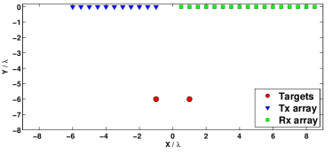
Figure 1: Geometry for the considered imaging problem in 2-D space.

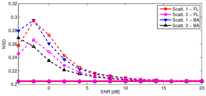
Figure 2: NSD (generalized null spectrum) vs. SNR; theoretical (Eq. (24), solid lines) vs. MC-based (dashed lines) performance.

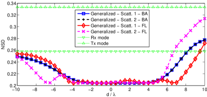
Figure 3: Theoretical NSD vs. scatterers rigid shift $d$; two targets located at $(\bm{x}_{1}/\lambda)=\left[\begin{array}[]{cc}(-1-d)&-6\end{array}\right]^{T}$ and $(\bm{x}_{2}/\lambda)=\left[\begin{array}[]{cc}(1-d)&-6\end{array}\right]^{T}$.

IV Numerical results

In this section we confirm our findings through simulations, focusing on 2-D localization, with Green function being $\mathcal{G}(\bm{x}^{\prime},\bm{x})=H_{0}^{(1)}\left(\kappa\left\|\bm{x}^{\prime}-\bm{x}\right\|\right)$. Here $H_{n}^{(1)}(\cdot)$ and $\kappa=2\pi/\lambda$ denote the $n$th order Hankel function of the 1st kind and the wavenumber ($\lambda$ is the wavelength), respectively. First, we consider a setup with $\lambda/2$-spaced Tx/Rx arrays ($N_{T}=11$ and $N_{R}=17$, respectively, see Fig. 1). Secondly, to quantify the level of multiple scattering (as in [8]) we define the index $\eta\triangleq\left\|\bm{K}_{\mathrm{f}}(\bm{x}_{1:M},\bm{\tau})-\bm{K}_{\mathrm{b}}(\bm{x}_{1:M},\bm{\tau})\right\|_{F}/\left\|\bm{K}_{\mathrm{b}}(\bm{x}_{1:M},\bm{\tau})\right\|_{F},$ where $\bm{K}_{\mathrm{b}}(\bm{x}_{1:M},\bm{\tau})$ and $\bm{K}_{\mathrm{f}}(\bm{x}_{1:M},\bm{\tau})$ denote the MDMs generated via BA and FL models, respectively. Finally, for simplicity we consider $M=2$ targets located at $(\bm{x}_{1}/\lambda)=\left[\begin{array}[]{cc}-1&-6\end{array}\right]^{T}$ and $(\bm{x}_{2}/\lambda)=\left[\begin{array}[]{cc}+1&-6\end{array}\right]^{T}$ and having scattering coefficients $\bm{\tau}=\left[\begin{array}[]{cc}3&4\end{array}\right]^{T}$; thus $\eta=(0.7445)$.

Then, we compare the asymptotic NSD (Eq. (24), solid lines) with the true ones obtained via Monte Carlo (MC) simulation (dashed lines, $10^{5}$ runs), focusing only on the generalized null-spectrum for brevity. To this end, Fig. 2 depicts the null-spectrum NSD vs. SNR for the two targets being considered, both for FL and BA models. It is apparent that, as the SNR increases, the theoretical results tightly approximate the MC-based ones, with approximations deemed accurate above $\mathrm{SNR}\approx 10\,\mathrm{dB}$. Differently, in Fig. 3, we plot the asymptotic NSD of the three TR-MUSIC variants vs. $d$, where $(\bm{x}_{1}/\lambda)=\left[\begin{array}[]{cc}(-1-d)&-6\end{array}\right]^{T}$ and $(\bm{x}_{2}/\lambda)=\left[\begin{array}[]{cc}(1-d)&-6\end{array}\right]^{T}$ (i.e. a rigid shift of the two scatterers), in order to investigate the potentially improved asymptotic stability (viz. NSD) of the generalized spectrum in comparison to Tx and Rx modes. It is apparent that the gain is significant when $d\in(-5,5)$, while outside this interval the NSD expression is either dominated by Tx or Rx mode, which for the present case $\mathrm{NSD}_{\mathrm{t},k}=1/\sqrt{11-2}\approx 0.33$ and $\mathrm{NSD}_{\mathrm{r},k}=1/\sqrt{17-2}\approx 0.26$, with the generalized NSD never above that of $\mathrm{NSD}_{\mathrm{t},k}$ (as dictated from Eq. (25)).

V Conclusions

We provided an asymptotic (high-SNR) analysis of TR-MUSIC null-spectrum in a non-colocated multistatic setup, by taking advantage of the 1st-order perturbation of the SVD of the MDM. Three different variants of TR-MUSIC were analyzed (i.e. Tx mode, Rx mode and generalized), based on the characterization of a certain complex-valued Gaussian vector. This allowed to obtain the asymptotic NSD (a measure of null-spectrum stability) for all the three imaging procedures. While similar results as the DOA setup were obtained for Tx and Rx modes, it was shown a clear dependence of generalized null-spectrum NSD on the scatterer and measurement setup. Finally, its potential stability advantage was investigated in comparison to Tx and Rx modes. Future works will analyze mutual coupling, antenna pattern and polarization effects [35, 36], and propagation in inhomogeneous (random) media [37].

References

• [1] M. Fink, “Time-reversal mirrors,” Journal of Physics D: Applied Physics, vol. 26, no. 9, p. 1333, 1993.
• [2] D. Cassereau and M. Fink, “Time-reversal of ultrasonic fields. III. theory of the closed time-reversal cavity,” IEEE Trans. Ultrason., Ferroelectr., Freq. Control, vol. 39, no. 5, pp. 579–592, Sep. 1992.
• [3] G. Micolau, M. Saillard, and P. Borderies, “DORT method as applied to ultrawideband signals for detection of buried objects,” IEEE Trans. Geosci. Remote Sens., vol. 41, no. 8, pp. 1813–1820, Aug. 2003.
• [4] L. Li, W. Zhang, and F. Li, “A novel autofocusing approach for real-time through-wall imaging under unknown wall characteristics,” IEEE Trans. Geosci. Remote Sens., vol. 48, no. 1, pp. 423–431, Jan. 2010.
• [5] M. D. Hossain, A. S. Mohan, and M. J. Abedin, “Beamspace time-reversal microwave imaging for breast cancer detection,” IEEE Antennas Wireless Propag. Lett., vol. 12, pp. 241–244, 2013.
• [6] C. Prada, S. Manneville, D. Spoliansky, and M. Fink, “Decomposition of the time reversal operator: Detection and selective focusing on two scatterers,” The Journal of the Acoustical Society of America, vol. 99, no. 4, pp. 2067–2076, 1996.
• [7] A. J. Devaney, “Time reversal imaging of obscured targets from multistatic data,” IEEE Trans. Antennas Propag., vol. 53, no. 5, pp. 1600–1610, May 2005.
• [8] E. A. Marengo and F. K. Gruber, “Subspace-based localization and inverse scattering of multiply scattering point targets,” EURASIP Journal on Advances in Signal Processing, pp. 1–16, 2007.
• [9] E. A. Marengo, F. K. Gruber, and F. Simonetti, “Time-reversal MUSIC imaging of extended targets,” IEEE Trans. Image Process., vol. 16, no. 8, pp. 1967–1984, Aug. 2007.
• [10] R. Schmidt, “Multiple emitter location and signal parameter estimation,” IEEE Trans. Antennas Propag., vol. 34, no. 3, pp. 276–280, 1986.
• [11] M. Kaveh and A. Barabell, “The statistical performance of the MUSIC and the minimum-norm algorithms in resolving plane waves in noise,” IEEE Trans. Acoust., Speech, Signal Process., vol. 34, no. 2, pp. 331–341, 1986.
• [12] B. Friedlander, “A sensitivity analysis of the MUSIC algorithm,” IEEE Trans. Acoust., Speech, Signal Process., vol. 38, no. 10, pp. 1740–1751, Oct. 1990.
• [13] B. Porat and B. Friedlander, “Analysis of the asymptotic relative efficiency of the MUSIC algorithm,” IEEE Trans. Acoust., Speech, Signal Process., vol. 36, no. 4, pp. 532–544, Apr. 1988.
• [14] P. Stoica and A. Nehorai, “MUSIC, maximum likelihood, and Cramér-Rao bound,” IEEE Trans. Acoust., Speech, Signal Process., vol. 37, no. 5, pp. 720–741, May 1989.
• [15] F. Li and R. J. Vaccaro, “Analysis of min-norm and MUSIC with arbitrary array geometry,” IEEE Trans. Aerosp. Electron. Syst., vol. 26, no. 6, pp. 976–985, 1990.
• [16] A. L. Swindlehurst and T. Kailath, “A performance analysis of subspace-based methods in the presence of model errors, Part I: the MUSIC algorithm,” IEEE Trans. Signal Process., vol. 40, no. 7, pp. 1758–1774, Jul. 1992.
• [17] A. Ferréol, P. Larzabal, and M. Viberg, “On the asymptotic performance analysis of subspace DOA estimation in the presence of modeling errors: case of MUSIC,” IEEE Trans. Signal Process., vol. 54, no. 3, pp. 907–920, Mar. 2006.
• [18] ——, “On the resolution probability of MUSIC in presence of modeling errors,” IEEE Trans. Signal Process., vol. 56, no. 5, pp. 1945–1953, May 2008.
• [19] ——, “Statistical analysis of the MUSIC algorithm in the presence of modeling errors, taking into account the resolution probability,” IEEE Trans. Signal Process., vol. 58, no. 8, pp. 4156–4166, Aug. 2010.
• [20] D. Ciuonzo, G. Romano, and R. Solimene, “On MSE performance of time-reversal MUSIC,” in IEEE 8th Sensor Array and Multichannel Signal Processing Workshop (SAM), Jun. 2014, pp. 13–16.
• [21] ——, “Performance analysis of time-reversal MUSIC,” IEEE Trans. Signal Process., vol. 63, no. 10, pp. 2650–2662, 2015.
• [22] G. Shi and A. Nehorai, “Cramér-Rao bound analysis on multiple scattering in multistatic point-scatterer estimation,” IEEE Trans. Signal Process., vol. 55, no. 6, pp. 2840–2850, Jun. 2007.
• [23] J. Choi and I. Song, “Asymptotic distribution of the MUSIC null spectrum,” IEEE Trans. Signal Process., vol. 41, no. 2, pp. 985–988, 1993.
• [24] F. Li, H. Liu, and R. J. Vaccaro, “Performance analysis for DOA estimation algorithms: unification, simplification, and observations,” IEEE Trans. Aerosp. Electron. Syst., vol. 29, no. 4, pp. 1170–1184, 1993.
• [25] D. Ciuonzo and P. Salvo Rossi, “On the asymptotic distribution of time-reversal MUSIC null spectrum,” Elsevier Digital Signal Processing, submitted, 2016.
• [26] E. G. Asgedom, L.-J. Gelius, A. Austeng, S. Holm, and M. Tygel, “Time-reversal multiple signal classification in case of noise: A phase-coherent approach,” The Journal of the Acoustical Society of America, vol. 130, no. 4, pp. 2024–2034, 2011.
• [27] M. E. Yavuz and F. L. Teixeira, “On the sensitivity of time-reversal imaging techniques to model perturbations,” IEEE Transactions on Antennas and Propagation, vol. 56, no. 3, pp. 834–843, Mar. 2008.
• [28] A. C. Fannjiang, “The MUSIC algorithm for sparse objects: a compressed sensing analysis,” Inverse Problems, vol. 27, no. 3, p. 035013, 2011.
• [29] H. Krim and M. Viberg, “Two decades of array signal processing research: the parametric approach,” IEEE Signal Process. Mag., vol. 13, no. 4, pp. 67–94, 1996.
• [30] G. Shi and A. Nehorai, “Maximum likelihood estimation of point scatterers for computational time-reversal imaging,” Communications in Information & Systems, vol. 5, no. 2, pp. 227–256, 2005.
• [31] G. W. Stewart, “Error and perturbation bounds for subspaces associated with certain eigenvalue problems,” SIAM review, vol. 15, no. 4, pp. 727–764, 1973.
• [32] J. Liu, X. Liu, and X. Ma, “First-order perturbation analysis of singular vectors in singular value decomposition,” IEEE Trans. Signal Process., vol. 56, no. 7, pp. 3044–3049, Jul. 2008.
• [33] D. S. Bernstein, Matrix mathematics: theory, facts, and formulas.   Princeton University Press, 2009.
• [34] P. J. Schreier and L. L. Scharf, Statistical Signal Processing of Complex-Valued Data: The Theory of Improper and Noncircular Signal.   Cambridge, 2010.
• [35] K. Agarwal and X. Chen, “Applicability of MUSIC-type imaging in two-dimensional electromagnetic inverse problems,” IEEE Trans. Antennas Propag., vol. 56, no. 10, pp. 3217–3223, 2008.
• [36] R. Solimene and A. Dell’Aversano, “Some remarks on time-reversal MUSIC for two-dimensional thin PEC scatterers,” IEEE Geoscience and Remote Sensing Letters, vol. 11, no. 6, pp. 1163–1167, Jun. 2014.
• [37] A. E. Fouda and F. L. Teixeira, “Statistical stability of ultrawideband time-reversal imaging in random media,” IEEE Transactions on Geoscience and Remote Sensing, vol. 52, no. 2, pp. 870–879, Feb. 2014.