Möbius domain-wall fermions on gradient-flowed dynamical HISQ ensembles

Abstract

We report on salient features of a mixed lattice QCD action using valence Möbius domain-wall fermions solved on the dynamical $N_{f}=2+1+1$ HISQ ensembles generated by the MILC Collaboration. The approximate chiral symmetry properties of the valence fermions are shown to be significantly improved by utilizing the gradient-flow scheme to first smear the HISQ configurations. The greater numerical cost of the Möbius domain-wall inversions is mitigated by the highly efficient QUDA library optimized for NVIDIA GPU accelerated compute nodes. We have created an interface to this optimized QUDA solver in Chroma. We provide tuned parameters of the action and performance of QUDA using ensembles with the lattice spacings $a\simeq\{0.15,0.12,0.09\}$ fm and pion masses $m_{\pi}\simeq\{310,220,130\}$ MeV. We have additionally generated two new ensembles with $a\sim 0.12$ fm and $m_{\pi}\sim\{400,350\}$ MeV. With a fixed flow-time of $t_{gf}=1$ in lattice units, the residual chiral symmetry breaking of the valence fermions is kept below 10% of the light quark mass on all ensembles, $m_{res}\lesssim 0.1\times m_{l}$, with moderate values of the fifth dimension $L_{5}$ and a domain-wall height $M_{5}\leq 1.3$. As a benchmark calculation, we perform a continuum, infinite volume, physical pion and kaon mass extrapolation of $F_{K^{\pm}}/F_{\pi^{\pm}}$ and demonstrate our results are independent of flow-time, and consistent with the FLAG determination of this quantity at the level of less than one standard deviation.

I Introduction

QCD (Quantum Chromodynamics) Fritzsch and Gell-Mann (1972); Fritzsch et al. (1973) is the fundamental theory of the strong interaction, and one of the three gauge theories of the SM (Standard Model) of particle physics. QCD encodes the interactions between quarks and gluons, the constituents of strongly interacting matter, which both carry color charges of QCD. At short distances, the quarks and gluons perturbatively interact with a coupling strength that runs to zero in the UV (ultraviolet) limit Gross and Wilczek (1973); Politzer (1973). Conversely, at long distance/low energy, the IR (infrared) regime, the coupling becomes $\mathcal{O}(1)$, and QCD becomes a strongly coupled theory. Consequently, the quarks and gluons are confined into the colorless hadrons we observe in nature, such as the proton, neutron, pions, etc. In order to compute properties of nucleons, nuclei, and other strongly interacting matter directly from QCD, we must therefore use a nonperturbative regularization scheme.

Asymptotic freedom, the property in which the gauge coupling becomes perturbative in the UV, makes the theory perfectly amenable to a numerical approach. QCD can be constructed on a discrete, Euclidean spacetime lattice, with a technique known as LQCD (lattice QCD). As the discretization scale is made sufficiently fine and the coupling becomes perturbative, the lattice action can be matched onto the continuum action to a desired order in perturbation theory. To aid the matching, EFT (Effective Field Theory) Weinberg (1979) can be used to perform an expansion of the lattice action in powers of the discretization scale, typically denoted $a$, which is referred to as the Symanzik expansion Symanzik (1983a, b). There are many different choices for constructing the discretized action, each of which corresponds to a different lattice action. As the continuum limit is taken, the difference between these lattice actions vanishes as the only dimension-4 operators allowed by the symmetries are those of QCD: the discretization effects, which include Lorentz violating interactions, are all described by irrelevant operators in the Symanzik expansion. An important test of this universality is to perform calculations of various physical quantities, with different lattice actions, and show consistency between them in the continuum limit. This is now routinely done for mesonic quantities and reviewed every two to three years by the FLAG Working Group, with the latest review in Ref. Aoki et al. (2017).

Lattice gauge theory began with the formulation of gauge fields on a spacetime lattice as originally proposed by Wilson Wilson (1974). The inclusion of fermions presents further challenges. The naive discretization of the fermion action leads to the fermion doubling problem, in which there are $2^{D}$ fermions in $D$ dimensions for each fermion field implemented. These doublers arise from the periodicity of the lattice action in momentum space and the single derivative in the Dirac equation. Wilson proposed the original method, now known as the Wilson fermion action, to remove these doublers by adding an irrelevant operator to the action which provides an additive mass to the doublers which scales as $1/a$. This irrelevant operator breaks chiral symmetry and requires fine-tuning the bare fermion mass to simulate a theory with light fermions, such as QCD with light $up$ and $down$ quarks. Despite (or because of) its simplicity, the Wilson fermion action is still one of the most popular in use. These days, the leading $\mathcal{O}(a)$ discretization corrections are removed perturbatively or nonperturbatively through an additional dimension-5 operator, the clover operator $c_{SW}\,a\bar{q}{\sigma}_{\mu\nu}G_{\mu\nu}q$, in what is known as the Wilson-Clover or Clover fermion action. The parameter $c_{SW}$ is the Sheikholeslami-Wohlert coefficient Sheikholeslami and Wohlert (1985) which can be tuned to remove the $\mathcal{O}(a)$ discretization effects from correlation functions. The idea has also been extended to twisted mass Wilson fermions Frezzotti et al. (2001), in which a complex quark-mass term is used, allowing for automatic ${\mathcal{O}}(a)$ improvement of physical observables provided the theory is computed at maximal twist Frezzotti and Rossi (2004).

Another common lattice action is known as the Kogut-Susskind or staggered fermion action Kogut and Susskind (1975); Susskind (1977). This action reduces the number of fermion doublers by exploiting a symmetry of the naive fermion action. A suitable spacetime-dependent phase rotation of the fermion fields allows for the Dirac equation to be diagonalized, thereby reducing the number of doublers from 16 to 4, in four spacetime dimensions. To perform numerical simulations with just one or two light fermion flavors, a fourth or square root of the fermion determinant is used Marinari et al. (1981). This rooting leads to nonlocal interactions at finite lattice spacing Bernard et al. (2007, 2006); Creutz (2007); however, perturbation theory Bernard (2005, 2006), the renormalization group Shamir (2005, 2007); Bernard et al. (2008a), and numerical simulations Durr and Hoelbling (2005, 2006); Hasenfratz and Hoffmann (2006), have been used to argue that these nonlocal effects vanish in the continuum limit. While this has not been proven nonperturbatively, some of the potential sicknesses of the theory can be shown to be the same as those of partially quenched lattice QCD Bernard et al. (2008b), which we will discuss briefly in short order. While not universally accepted, all numerical evidence suggests that rooted-staggered LQCD is in the same universality class as QCD as the continuum limit is taken Sharpe (2006); Kronfeld (2007); Bazavov et al. (2010a); Aoki et al. (2017).

Determining a nonperturbative regulator that both preserves chiral symmetry and has the correct number of light degrees of freedom is challenging. It has been shown that in four spacetime dimensions, one cannot simultaneously have all four of the conditions: chiral symmetry, ultralocal action, undoubled fermions, and the correct continuum limit. This is known as the Nielsen-Ninomiya no-go theorem Nielsen and Ninomiya (1981a, b, c). However, one can extend the definition of chiral symmetry at finite lattice spacing: if the lattice Dirac operator, $D$, satisfies the Ginsparg-Wilson relation Ginsparg and Wilson (1982)

$$\left\{{\gamma}_{5},D\right\}=aD{\gamma}_{5}D\,,$$ (1)

it will respect chiral symmetry even at finite lattice spacing Lüscher (1998). One consequence is the theory will be automatically $\mathcal{O}(a)$ improved as the only nontrivial dimension-5 operator that cannot be removed through field redefinitions and equations of motion is the clover operator, which explicitly breaks chiral symmetry and is thus not allowed. There are two lattice actions which satisfy the Ginsparg-Wilson relation: the DW (domain-wall) fermion action Kaplan (1992); Shamir (1993); Furman and Shamir (1995) and the overlap fermion action Narayanan and Neuberger (1994, 1993, 1995). The DW fermion action is formulated with a finite fifth dimension of extent $L_{5}$, where the left and right chiral modes are bound to opposite ends of the fifth dimension. The gluon action is a trivial copy of the 4D action on each fifth-dimensional slice with unit link variable between the slices, and so the fermions have only a simple kinetic action in the fifth dimension. At finite $L_{5}$, the left and right modes have a nonvanishing overlap due to fermion modes which propagate into the fifth dimension. The massive modes decay exponentially in the fifth dimension, while the fermion zero modes have only a power-law falloff. This small overlap leads to a small, residual breaking of chiral symmetry at finite $L_{5}$, characterized by a quantity known as $m_{res}$. The overlap fermion action can be shown to be equivalent to the domain-wall action as $L_{5}\rightarrow\infty$ Borici (2000, 1999) and respects chiral symmetry to a desired numerical precision.

The numerical cost of generating lattice ensembles with domain-wall and overlap actions is 1 or more orders of magnitude greater than the cost of generating ensembles with Wilson-type or staggered fermion actions Kennedy (2005). This has led to interest in, and the development of, mixed lattice actions or MA (mixed-actions) Bar et al. (2003), in which the valence and sea-quark lattice actions are not the same at finite lattice spacing. In the most common MALQCD calculations, the dynamical sea-quark action is generated with a numerically less expensive discretization scheme, such as staggered- or Wilson-type fermions, while the valence-quark action, which is used to construct correlation functions, is implemented with domain-wall or overlap fermions, thus retaining the full chiral symmetry in the valence sector. The first implementation of a MALQCD calculation was performed by the LHP Collaboration Renner et al. (2005) utilizing DW fermions on the publicly available asqtad ($a^{2}$ tadpole improved) Orginos and Toussaint (1999); Orginos et al. (1999) rooted staggered ensembles generated by the MILC Collaboration Bernard et al. (2001); Bazavov et al. (2010a). A number of important results were obtained with this particular MALQCD setup, including the first dynamical calculation of the nucleon axial charge with light pion masses Edwards et al. (2006) and more general nucleon structure Hagler et al. (2008); Bratt et al. (2010), the first dynamical calculation of two-nucleon elastic scattering Beane et al. (2006), a precise calculation of the $I=2\ \pi\pi$ scattering length Beane et al. (2008), a detailed study of the quark-mass dependence of the light baryon spectrum Walker-Loud et al. (2009), a calculation of the kaon bag parameter with fully controlled uncertainties Aubin et al. (2010), and many more.

The predominant reason for the success of these MALQCD calculations is the good chiral symmetry properties of the DW action, which significantly suppresses chiral symmetry breaking from the staggered sea fermions and discretization effects. EFT can be used to understand the salient features of such MALQCD calculations. $\chi$PT (Chiral Perturbation Theory) Langacker and Pagels (1973); Gasser and Leutwyler (1984); Leutwyler (1994) can be extended to incorporate discretization effects into the analytic formulae describing the quark-mass dependence of various hadronic quantities. The procedure is to first construct the local Symanzik action for a given lattice action and then to use spurion analysis to construct all operators in the low-energy EFT describing such a lattice action, including contributions from higher-dimension operators Sharpe and Singleton (1998). The MAEFT Bar et al. (2004) for DW valence fermions on dynamical rooted staggered fermions is well developed Bar et al. (2005); Tiburzi (2005a); Chen et al. (2006, 2007); Orginos and Walker-Loud (2008); Jiang (2007); Chen et al. (2009a, b). The use of valence fermions which respect chiral symmetry leads to a universal form of the MAEFT extrapolation formulae at NLO (next-to-leading order) in the dual quark-mass and lattice spacing expansions Chen et al. (2007, 2009a). This universal behavior follows from the suppression of chiral symmetry breaking discretization effects from the sea sector when constructing correlation functions from valence fermions. Further, quantities which are protected by chiral symmetry are free of new LECs (low-energy constants) at NLO provided on-shell renormalized quantities are used in the extrapolation formulae Chen et al. (2006, 2007). This universality allows for the derivation of NLO MAEFT formula directly from their PQ$\chi$PT (partially quenched $\chi$PT) Bernard and Golterman (1994); Sharpe and Shoresh (2000, 2001); Chen and Savage (2002); Sharpe and Van de Water (2004); Arndt and Tiburzi (2003a); Walker-Loud (2005); Bernard and Golterman (2010, 2013) counterparts, provided they are known Beane and Savage (2002, 2003); Arndt and Tiburzi (2003b, 2004); Tiburzi and Walker-Loud (2005); Tiburzi (2005b); Tiburzi and Walker-Loud (2006); O’Connell and Savage (2006). MALQCD calculations with DW valence quarks on the asqtad rooted staggered ensembles have been stress tested through a comparison of quantities which are directly sensitive to the unitarity violations present in MALQCD calculations, in particular the $a_{0}$ meson correlation function Prelovsek (2006); Aubin et al. (2008). There are a few other MA constructions that have been tested, but only a few others that are actively used. The HPQCD Collaboration utilizes HISQ (highly improved staggered quark) valence fermions on the asqtad ensembles; for example, see Refs. Na et al. (2015); Donald et al. (2014). The $\chi$QCD Collaboration utilizes overlap valence fermions on the dynamical $N_{f}=2+1$ domain-wall ensembles Li et al. (2010); Lujan et al. (2012); Gong et al. (2013) generated by the RBC/UKQCD Collaboration Allton et al. (2007); Aoki et al. (2011). The work in Refs. Basak et al. (2012, 2014, 2015); Mathur et al. (2016) uses valence overlap fermions on the $N_{f}=2+1+1$ HISQ ensembles Bhattacharya et al. (2014). The PNDME Collaboration has utilized clover improved valence fermions on the $N_{f}=2+1+1$ HISQ ensembles Bhattacharya et al. (2014, 2015). While this MA choice is economical, it does not benefit from the suppression of chiral symmetry breaking discretization effects as with the DW on asqtad or overlap on DW MALQCD calculations.

Given the successes described above, MALQCD provides an economical means of performing LQCD calculations in which chiral symmetry breaking effects are highly suppressed by utilizing a valence fermion action that respects chiral symmetry in combination with a set of LQCD ensembles that do not, but are less numerically expensive to generate. In this article, we motivate a new MALQCD action and present numerical evidence for salient features of the action.

II Möbius Domain-Wall fermions on gradient-flowed HISQ ensembles

Table 1: The HISQ ensembles used in this work and planned for future MALQCD calculations. In addition to the pion mass and lattice spacing, we list the number of configurations used in the present work, $N_{cfg}$ as well as the Monte Carlo time, ${\Delta}{\tau}_{MC}$, by which the configurations were separated in this work. The short name, introduced in Ref. Bhattacharya et al. (2015), is for brevity. The last two HISQ ensembles were generated at LLNL targeting heavier pion masses to test the radius of convergence of the chiral extrapolation in future MALQCD calculations.

Short	Ensemble	$am_{\pi}^{HISQ-5}$	$am_{ss}^{HISQ-5}$	Volume	$\sim a$	$\sim m_{\pi}$	$m_{\pi}L$	$N_{cfg}$	${\Delta}{\tau}_{MC}$
name					[fm]	[MeV]
a15m310	l1648f211b580m013m065m838a	0.23646(17)	0.51858(17)	$16^{3}\times 48$	0.15	310	3.78	196	50
a12m310	l2464f211b600m0102m0509m635a	0.18931(10)	0.41818(10)	$24^{3}\times 64$	0.12	310	4.54	199	25
a09m310	l3296f211b630m0074m037m440e	0.14066(13)	0.31133(12)	$32^{3}\times 96$	0.09	310	4.50	196	24
a15m220	l2448f211b580m0064m0640m828a	0.16612(08)	0.51237(10)	$24^{3}\times 48$	0.15	220	3.99	199	25
a12m220	l3264f211b600m00507m0507m628a	0.13407(06)	0.41559(07)	$32^{3}\times 64$	0.12	220	4.29	199	25
a09m220	l4896f211b630m00363m0363m430a	0.09849(07)	0.30667(07)	$48^{3}\times 96$	0.09	220	4.73	–	–
a15m130	l3248f211b580m00235m0647m831a	0.10161(06)	0.51427(05)	$32^{3}\times 48$	0.15	130	3.25	–	–
a12m130	l4864f211b600m00184m0507m628a	0.08153(04)	0.41475(05)	$48^{3}\times 64$	0.12	130	3.91	–	–
a12m400	l2464f211b600m0170m0509m635a	0.24398(12)	0.41970(12)	$24^{3}\times 64$	0.12	400	5.86	–	–
a12m350	l2464f211b600m0130m0509m635a	0.21376(13)	0.41923(13)	$24^{3}\times 64$	0.12	350	5.13	–	–

Present-day LQCD calculations for mesonic quantities are performed with multiple lattice spacings, multiple volumes and physical pion masses, allowing for complete control over all LQCD systematics, see Ref. Aoki et al. (2017) for many examples. The simplest single baryon properties are also computed with multiple lattice spacings/volumes and near-physical and sometimes physical pion masses Durr et al. (2012, 2016); Yang et al. (2016); Sufian et al. (2017), including the first calculation of the nucleon axial charge with both physical pion masses and a continuum limit Bhattacharya et al. (2016) and isospin violating corrections Borsanyi et al. (2013, 2015); Bhattacharya et al. (2016); Brantley et al. (2016). If one is interested in a set of ensembles allowing for this much control over LQCD systematics, there are only two such sets publicly available, both of which are generated and provided by the MILC Collaboration: the $N_{f}=2+1$ asqtad ensembles Bazavov et al. (2010a) and the $N_{f}=2+1+1$ HISQ Follana et al. (2007) ensembles generated more recently Bazavov et al. (2010b, 2013). The HISQ ensembles have taste splittings in the pseudoscalar sector that are one generation finer in discretization Bazavov et al. (2013), such that the $a\sim 0.15$ fm HISQ ensemble taste violations are similar in size to the $a\sim 0.12$ fm asqtad ensembles. There is a vast set of HISQ ensembles with $130\lesssim m_{\pi}\lesssim 310$ MeV, strange and charm quark masses tuned near their physical values and lattice spacings of $a\sim\{0.15,0.12,0.09,0.06,0.042,0.03\}$ fm, including multiple spatial volumes and lighter than physical strange quark masses. In addition to the publicly available HISQ ensembles, we have generated two additional sets at $a\sim 0.12$ fm and $m_{\pi}\approx 350,\ 400$ MeV with fixed volume in lattice units such that $m_{\pi}L\geq 5.1$. In Table 1, we list the HISQ ensembles utilized in the present work as well as ensembles for which we have tuned the MDWF parameters for future work.

Given the great success of the MA DW fermion on asqtad LQCD calculations Edwards et al. (2006); Hagler et al. (2008); Bratt et al. (2010); Beane et al. (2006, 2008); Walker-Loud et al. (2009); Aubin et al. (2010), we have chosen to use DW fermions for the present MALQCD calculations as well. In the present work, we have chosen to use the MDWF (Möbius DW fermion) action Brower et al. (2005, 2006, 2012) which offers reduced residual chiral symmetry breaking at fixed fifth-dimensional extent, $L_{5}$. With the introduction of two new parameters, $b_{5}$ and $c_{5}$, the Möbius kernel can be smoothly interpolated between the Shamir Shamir (1993) and the Neuberger/Boriçi Neuberger (1998a, b); Borici (2000, 1999) kernels. Following Ref. Brower et al. (2012), the Möbius kernel can be expressed as

$$D^{\textrm{M\"{o}bius}}(M_{5})=\frac{(b_{5}+c_{5})D^{\textrm{Wilson}}(M_{5})}{2+(b_{5}-c_{5})D^{\textrm{Wilson}}(M_{5})}\,.$$ (2)

Alternatives include a polar decomposition to the sign function Vranas (1998); Kikukawa and Noguchi (2000); Edwards and Heller (2001) or other methods of approximating the sign function Kennedy (2006). In this work, we have always chosen values of $b_{5}$ and $c_{5}$ with the constraint $b_{5}-c_{5}=1$, such that the Möbius kernel is a rescaled version of the Shamir kernel

$$D^{\textrm{M\"{o}bius}}(M_{5})=\frac{\alpha D^{\textrm{Wilson}}(M_{5})}{2+D^{\textrm{Wilson}}(M_{5})}\equiv\alpha D^{\textrm{Shamir}}(M_{5}).$$ (3)

It was demonstrated in Ref. Brower et al. (2012) that this rescaling factor, $\alpha$, exponentially enhances the suppression of residual chiral symmetry breaking as

$$m_{res}\sim e^{-\alpha L_{5}}\,,$$ (4)

provided the action is in a regime where these exponentially damped terms are the dominant contribution to $m_{res}$ and $\alpha$ is not too large, but of the order $\alpha\sim 2-4$. With the constraint $b_{5}-c_{5}=1$, the rescaling factor is given by $\alpha=b_{5}+c_{5}$.

III Gradient-flow smearing

From the DW on asqtad action Edwards and Joo (2005), it is known that the asqtad gauge fields required additional levels of smearing to reduce the residual chiral symmetry breaking. For that action, HYP smearing Hasenfratz and Knechtli (2001); DeGrand et al. (2003); DeGrand (2004); Durr et al. (2004) was utilized for this purpose. In this work, we choose to investigate the use of the gradient flow Narayanan and Neuberger (2006); Lüscher and Weisz (2011); Lüscher (2013) as a smearing method. The gradient flow is a nonperturbative, classical evolution of the original fields in a new parameter, the flow-time, that drives those fields toward a classical minimum. In real space, this corresponds to smearing out the degrees of freedom through an infinitesimal stout-smearing procedure Morningstar and Peardon (2004).

Gradient flow smearing introduces a new scale, of the order $l_{gf}\sim\sqrt{8t_{gf}}\,a$, where $t_{gf}$ is the (dimensionless) flow-time. Correlation functions depend upon this new scale, which can serve as a nonperturbative, rotationally invariant UV regulator that provides the possibility for improved renormalization procedures for various LQCD matrix elements Del Debbio et al. (2013); Suzuki (2013); Monahan and Orginos (2013); Lüscher (2014); Endo et al. (2015); Monahan and Orginos (2015, 2017). Here, however, we are interested in the gradient flow as a smearing algorithm Lüscher (2010); Lohmayer and Neuberger (2011).

To ensure that the continuum limit of LQCD matrix elements is free of any flow-time dependence, one must use a fixed flow-time in lattice units such that all flow-time dependence extrapolates to zero as the continuum limit is taken.

In this work, we have found that moderate values of the flow-time allow for a reduction of the residual chiral symmetry breaking such that $m_{res}<0.1\times m_{l}^{dwf}$ for moderate values of $L_{5}$. The resulting flow-time dependence of $m_{res}$ at fixed pion mass demonstrates that the gradient-flow highly suppresses the zero-mode contributions to $m_{res}$, such that an exponential dependence of $m_{res}$ on $L_{5}$ is recovered. Further, we have observed that gradient flow smearing has allowed us to use small values of the DW height, with $M_{5}\leq 1.3$ on all ensembles used in this work. This is important because with the larger values of $M_{5}$ used in the DW on asqtad calculations, there was strong contamination of the UV modes with an oscillatory time behavior, modes which are known to decouple as $M_{5}\rightarrow 1$ Syritsyn and Negele (2007). With the values of $M_{5}$ used in this work, there is no discernible contamination from these modes at larger flow-times.

We finally settled on a gradient flow-time of $t_{gf}=1.0$, which provided significant suppression of residual chiral symmetry breaking without introducing a large flow-time length scale. In the next section, we present detailed calculations showing the flow-time dependence of various quantities. This action has been used to compute the $\pi^{-}\rightarrow\pi^{+}$ matrix element relevant for neutrinoless double beta decay Nicholson et al. (2016) and also to perform an exploratory calculation of an improved method of computing hadronic matrix elements Bouchard et al. (2017) and an application to $g_{A}$ Berkowitz et al. (2017).

III.1 Tuning the action

Before showing results, we describe how to match the valence MDWF action and the HISQ action. With a given flow-time, our general algorithm for choosing values of the MDWF action parameters is:

1. For a fixed value of $L_{5}$, optimize $M_{5}$ to minimize the resulting value of $m_{res}$.

2. Vary the values of $L_{5}$, $b_{5}$ and $c_{5}$ under the constraints $b_{5}-c_{5}=1$ and $m_{res}\leq 0.1m_{l}^{dwf}$ while minimizing $L_{5}$.

3. Tune $m_{l}^{dwf}$ and $m_{s}^{dwf}$ such that $m_{\pi}^{dwf}\simeq m_{\pi}^{HISQ-5}$ and $m_{ss}^{dwf}\simeq m_{ss}^{HISQ-5}$ within ${\mathcal{O}}(2\%)$ or less where $HISQ-5$ denotes the taste-5 pseudoscalar mass of the dynamical HISQ action and $m_{ss}$ is the mass of the connected $\bar{s}{\gamma}_{5}s$ pseudoscalar meson.

This procedure required just a few iterations to converge to the desired results. For this work, we have used the definition of $m_{res}$ from the Shamir kernel as the residual chiral symmetry breaking between Shamir and Möbius becomes the same in the continuum limit Brower et al. (2012),

$$m_{res}(t)=\frac{\sum_{\mathbf{x}}\langle\bar{Q}(t,\mathbf{x}){\gamma}_{5}Q(t,\mathbf{x})\,\bar{q}(0,\mathbf{0}){\gamma}_{5}q(0,\mathbf{0}))\rangle}{\sum_{\mathbf{x}}\langle\bar{q}(t,\mathbf{x}){\gamma}_{5}q(t,\mathbf{x})\,\bar{q}(0,\mathbf{0}){\gamma}_{5}q(0,\mathbf{0}))\rangle}\,,$$ (5)

where $Q$ is a quark field in the midpoint of the fifth dimension and $q$ is a quark field bound to the domain wall.

In Table 2, we list the resulting MDWF parameters at the chosen gradient flow-time of $t_{gf}=1$. These parameters were used in Refs. Nicholson et al. (2016); Berkowitz et al. (2017).

Table 2: Tuned MDWF parameters for our MALQCD calculations. Some of the ensembles are used for example in Refs. Nicholson et al. (2016); Berkowitz et al. (2017).

Dnsemble	$M_{5}$	$L_{5}$	$b_{5}$	$c_{5}$	$t_{gf}$	$am_{l}^{mdwf}$	$am_{s}^{mdwf}$
a12m400	1.2	18	1.25	0.25	1.0	0.02190	0.0693
a12m350	1.2	18	1.25	0.25	1.0	0.01660	0.0693
a15m310	1.3	12	1.50	0.50	1.0	0.01580	0.0902
a12m310	1.2	18	1.25	0.25	1.0	0.01260	0.0693
a09m310	1.1	16	1.25	0.25	1.0	0.00951	0.0491
a15m220	1.3	16	1.75	0.75	1.0	0.00712	0.0902
a12m220	1.2	12	1.50	0.50	1.0	0.00600	0.0693
a09m220	1.1	18	1.25	0.25	1.0	0.00449	0.0491
a15m130	1.3	24	2.25	1.25	1.0	0.00216	0.0902
a12m130	1.2	20	2.00	1.00	1.0	0.00195	0.0693

IV Flow-time dependence of various quantities

To study the efficacy of this action, we compute the flow-time dependence of various quantities. In the next section we will show that the continuum limits of various ratios of physical quantities are flow-time independent. In order to test the flow-time dependence, we tune the input quark masses to hold the pion mass and the connected $ss$ pseudoscalar meson masses fixed within ${\mathcal{O}}(2\%)$. In the Appendix (Table 7), we list the tuned values of the input quark masses for various flow-times on the ensembles used in this work. We also list the resulting values of the plaquette, $m_{res}$, and the values of $Z_{A}$ determined as described below. In Fig. 1, we show the effective masses of the pion and nucleon, respectively, on the a15m310 ensemble for all flow-times. We observe that the contamination from oscillatory modes is suppressed at larger flow-times.

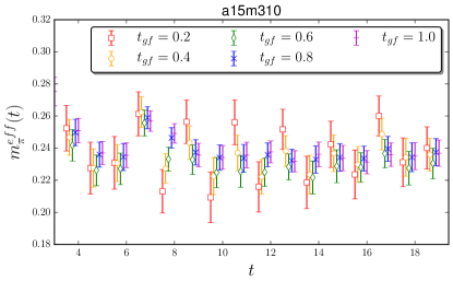
Figure 1: Effective mass of the pion (top) and proton (bottom) as a function of the Euclidean time $t$, at different flow-times on the a15m310 ensemble. The different flow-time values are slightly shifted horizontally for visual clarity.

From the input quark masses used at fixed pseudoscalar masses, and the average values of the plaquettes, one observes a substantial flow-time dependence of UV quantities. This is expected as the gradient flow smearing filters out the UV modes of the gauge fields. It is important to check the flow-time dependence of hadronic quantities and verify the continuum limit is flow-time independent. This can easily be checked with ratios of hadronic quantities. In Table 8, we list values of the meson masses, $m_{\pi}$, $m_{K}$ and $m_{ss}$ as well as the decay constants $F_{\pi}$ and $F_{K}$ and the nucleon mass $m_{N}$. We also provide the ratios of $F_{K}/F_{\pi}$ and $m_{N}/F_{\pi}$.

IV.1 Fit functions

To determine the value of $m_{res}$, we fit the correlation function described by Eq. (5) to a constant.

The meson correlation functions were folded in time to double the statistics while the nucleon correlation functions were averaged between the forward propagating positive parity interpolating operator and the backward propagating negative parity interpolating operator, constructed as in Refs. Basak et al. (2005a, b). The fit Ansatz describing a $\bar{q_{1}}q_{2}$-meson correlation functions is given by

$$C_{\textrm{2pt}}^{{q_{1}q_{2}}}(t)= \sum_{n}z^{q_{1}q_{2}}_{n}z^{q_{1}q_{2}\dagger}_{n}\left(e^{-E^{q_{1}q_{2}}_{n}t}+e^{-E^{q_{1}q_{2}}_{n}(T-t)}\right)$$

$$+(-1)^{t}z^{\textrm{osc.}}z^{\textrm{osc.}\dagger}\left(e^{-E^{\textrm{osc.}}t}+e^{-E^{\textrm{osc.}}(T-t)}\right),$$ (6)

where we define $z_{n}$ as the overlap factor of the $n$th state with energy $E_{n}$ and the superscript osc. denotes the overlap and energy of the oscillating mode.

In order to determine the pseudoscalar decay constants, we utilize the 5D Ward Identity relating the renormalized decay constants to various correlation functions including those used to determine the values of $m_{res}$ Blum et al. (2004); Aoki et al. (2004),

$$F^{q_{1}q_{2}}=z_{p}^{q_{1}q_{2}}\frac{m^{q_{1}}+m^{q_{1}}_{res}+m^{q_{2}}+m^{q_{2}}_{res}}{\sqrt[3]{E^{q_{1}q_{2}}_{0}}}\,,$$ (7)

where $z_{p}$ denotes the point-sink overlap factor. This normalization is such that the physical pion decay constant is $F_{\pi}=92.2$ MeV.

In order to determine the axial renormalization constants, we can also compute the bare values of $F^{q_{1}q_{2}}$ using the 4D axial-vector current,

$$C_{\textrm{axial}}^{q_{1}q_{2}}= \partial_{4}\langle 0|A_{4}(t)P_{S}(0)|0\rangle$$

$$= -\sum_{n}f^{q_{1}q_{2}}_{n}z_{s,n}^{q_{1}q_{2}}\left(e^{-E_{n}^{q_{1}q_{2}}t}+e^{-E_{n}^{q_{1}q_{2}}(T-t)}\right)$$

$$-(-1)^{t}f^{\textrm{osc.}}z^{\textrm{osc.}}_{s}\left(e^{-E^{\textrm{osc.}}t}+e^{-E^{\textrm{osc.}}(T-t)}\right)$$ (8)

where $f_{0}^{q_{1}q_{2}}=\sqrt{E_{0}^{q_{1}q_{2}}}F^{q_{1}q_{2}}/Z_{A}$ with renormalization coefficient $Z_{A}$ and $z_{s}$ is the same ground-state overlap factor determined in the two-point function.

For the nucleon two-point correlation function, we use the fit Ansatz analogous to Eq. (6) without the oscillating state and wraparound terms.

IV.2 Analysis strategy

The correlator analysis is performed using the Python package lsqfit Lepage (2016). We perform a chained fit Bouchard et al. (2014) to the light and strange $m_{res}$ correlator; the pion, kaon, and $\bar{s}{\gamma}_{5}s$-meson two-point and axial correlators; and the nucleon two-point correlator. In particular, as part of the chained fit, we perform a simultaneous fit to the pseudoscalar two-point (point- and smeared-sink) and axial correlators and to the nucleon point- and smeared-sink correlators. The chained fit implementation in lsqfit preserves all correlations by numerically implementing the propagation of error under the assumption that all parameters are Gaussian distributed. We use the resulting correlated posterior distributions to propagate all subsequent uncertainties (e.g. ratios) without performing any bootstrap resampling.

For the pseudoscalar correlators, we truncate the fit Ansatz at 2+1 states, where the +1 denotes the oscillating state. For the nucleon correlator, we perform a two-state fit. For the pseudoscalar correlators, in an independent analysis, using similar fit regions, we observe using three states without oscillating modes results in a consistent determination of the ground-state masses and overlap factors. Further, using an unconstrained, single-state fit in the late time region also results in consistent ground state parameters.

We choose unconstraining ground-state priors such that the prior widths are at least an order of magnitude wider than the width of the posterior distribution. The oscillating-state energy splitting is chosen to be at the lattice cutoff scale. The first excited-state energy splitting is chosen to be at the two-pion threshold. Details on our prior choices are given in Table 9.

The fit region is chosen such that $t_{\textrm{min}}\sim 1$ fm and $t_{\textrm{max}}\sim 2.3$ fm for all pseudoscalar correlators. For the nucleon correlator analysis, $t_{\textrm{min}}\sim 0.6$ fm and $t_{\textrm{max}}\sim 1.4$ fm are chosen for all ensembles. It is necessary to fit the nucleon correlator closer to the origin due to the poorer signal-to-noise ratio when compared to the pseudoscalar observables. Explicit fit regions in lattice units are given in Table 10. We observe that all final correlator fits are in the region of stability for varying $t_{\textrm{min}}$ and $t_{\textrm{max}}$, including the more aggressive nucleon analysis, indicating that the results are free of excited-state contamination.

IV.3 Observations about flow-time dependence

From our calculations, there are a few substantial benefits one observes from the use of the gradient-flow smearing. Before discussing these, we first comment on the strong oscillations observed at small flow-time in the pseudoscalar correlators. In Fig. 1, we observe a strong signal for an oscillating excited state with $(-1)^{t}$ behavior (where $t$ is the Euclidean time) at small flow-times, most notably for $t_{gf}=0.2$. These oscillating modes become completely damped out for $t_{gf}\geq 0.6$, with the statistics used in this work.

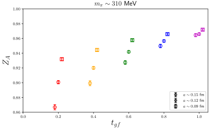
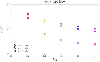
Figure 2: $Z_{A}$ (top) and $m_{l}^{res}$ (bottom) as a function of flow-time on the $m_{\pi}\simeq 310$ MeV ensembles. The results of $Z_{A}$ are slightly shifted horizontally for visual clarity.

The first significant benefit observed is that as the flow-time is increased a dramatic reduction of the chiral symmetry breaking properties of the valence MDWF action is achieved. This can be observed in the significant reduction in $m_{res}$ at fixed pion mass or similarly, the values of $Z_{A}$ approaching 1 for all gauge couplings, both of which are depicted in Fig. 2. With the tuning we have chosen, to hold the pion mass, as well as $L_{5}$, $M_{5}$, $b_{5}$, and $c_{5}$, fixed as we vary the flow-time, we observe an exponential reduction in $m_{res}$ as the flow-time is increased. Though not depicted in these figures or tables, we also studied the dependence of $m_{res}$ on $L_{5}$ as the flow-time was varied. We find that for small flow-time, the reduction in $m_{res}$ as $L_{5}$ increases is power law, indicating the 5D zero-mode contributions are dominating the residual chiral symmetry breaking. As we increase the flow-time, $m_{res}$ begins to fall off exponentially in $L_{5}$, indicating the gradient flow smearing suppresses these zero-mode contributions.

Another significant benefit we observe is that stochastic fluctuations become smaller for increasing flow-time because the gradient flow smearing procedure suppresses the ultraviolet noise. This is observed from the sample effective mass plots of the nucleon and pion in Fig. 1. The gradient flow is applied in all four spacetime directions, so the neighboring time slices become more correlated, rendering a direct comparison of the effective mass plots more complicated. However, the list of fitted quantities in Table 8 demonstrates the correlated stochastic uncertainties are reduced for increasing flow-time. Comparing the $t_{gf}=1$ to $t_{gf}=0.2$ results, we observe approximately a factor of $\sqrt{2}$ reduction of the stochastic uncertainty for equal computing cost for all quantities other than the pseudoscalar meson masses.

V Flow-time independence of continuum limit

In Fig. 3, we show a continuum study of $m_{N}/F_{\pi}$ and $F_{K}/F_{\pi}$ on the $m_{\pi}\sim 310$ MeV ensembles, for all flow-times used. We explore four different continuum extrapolation Ansätze for a quantity $f$:

$$f(a/w_{0})=\left\{\begin{array}[]{ll}f_{0}\,,&\textrm{constant\, ,}\\ f_{0}+f_{2}\frac{a^{2}}{w_{0}^{2}}\,,&\textrm{linear in $a^{2}$\, ,}\\ f_{0}+\alpha_{s}f_{2}^{\prime}\frac{a^{2}}{w_{0}^{2}}\,,&\textrm{linear in ${\alpha}_{s}a^{2}$\, ,}\\ f_{0}+f_{4}\frac{a^{4}}{w_{0}^{4}}\,,&\textrm{quadratic in $a^{2}$\, .}\end{array}\right.$$ (9)

The gradient flow scale $w_{0}$ was first defined in Ref. Borsanyi et al. (2012), and a value of $w_{0}\text{\cite[cite]{\@@bibref{Authors Phrase1YearPhrase2}{Borsanyi:2012zs}{\@@citephrase{(}}{\@@citephrase{)}}}}=0.1755(18)(04)$ fm was determined. The value determined in Ref. Bazavov et al. (2016a) is similar with a slight discrepancy, $w_{0}\text{\cite[cite]{\@@bibref{Authors Phrase1YearPhrase2}{Bazavov:2015yea}{\@@citephrase{(}}{\@@citephrase{)}}}}=0.1714({}_{12}^{15})$ fm. We use this value as we are using the same ensembles on which it was determined. With only three lattice spacings, we choose not to perform an extrapolation in both $a^{2}$ and either ${\alpha}_{s}a^{2}$ or $a^{4}$ simultaneously. However, we observe the value of $f_{2}$ for both $m_{N}/F_{\pi}$ and $F_{K}/F_{\pi}$ to be small and often consistent with zero. This motivates exploring the linear in ${\alpha}_{s}a^{2}$ and $a^{4}$ fits as estimates of systematic uncertainties in the continuum extrapolation. We find all four continuum extrapolations show consistency at the 1-sigma level, both between all four different fit Ansätze and also between the various flow-time extrapolations. In Fig. 3, we display the continuum extrapolation using the Ansatz linear in $(a/w_{0})^{2}$. The quark-mass-independent values of $a/w_{0}$ and ${\alpha}_{s}$ are taken from Ref. Bazavov et al. (2016a).

For $m_{N}/F_{\pi}$, we observe minimal discretization corrections with a very small slope in $(a/w_{0})^{2}$. For $F_{K}/F_{\pi}$, a quantity which is determined much more precisely for equal stochastic sampling, we observe mild, though still quite small, discretization corrections. While the discretization corrections are basically flow-time independent for $m_{N}/F_{\pi}$, they seem to become more pronounced for $F_{K}/F_{\pi}$ as the flow-time is increased. There is an indication of the presence of higher order quartic in $a/w_{0}$ corrections, but we are not able to resolve these with the numerical results in this work. Previous studies of the heavy-light decay constants observed that large amounts of APE smearing Albanese et al. (1987) could induce significant higher order discretization effects Bernard et al. (2002). It is possible that the larger $t_{gf}$ smearings are having a similar effect on the strange quark, and thus the value of $F_{K}$, at the sub percent level. These potential systematic uncertainties should be explored in more detail for a sub percent calculation of $F_{K}/F_{\pi}$ using this action.

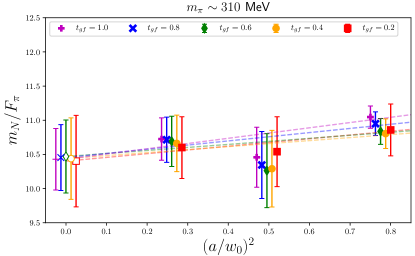
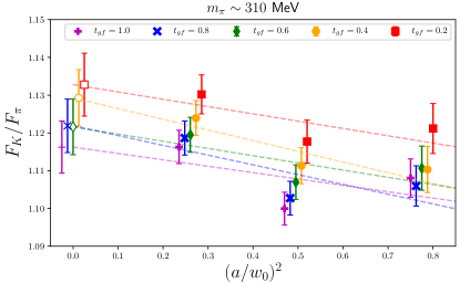
Figure 3: Flow-time (in)dependence of $m_{N}/F_{\pi}$ and $F_{K}/F_{\pi}$ on the $m_{\pi}\sim 310$ MeV ensembles. The filled in symbols are the results of our calculations, and the open symbols clustered at $a/w_{0}=0$ are the continuum extrapolated results using the simple Ansatz of a constant plus an $(a/w_{0})^{2}$ term. The results are slightly shifted horizontally for visual clarity.

V.1 Mixed-meson mass corrections

In order to use the MAEFT extrapolation formulae, there are a few additional quantities which must be determined from the MALQCD calculations. At NLO in the MAEFT expansion, one needs to know the masses of the mixed valence-sea mesons which propagate in virtual loops and the value of the partial quenching parameter which controls the unitarity violating contributions Chen et al. (2007, 2009a). In a general MALQCD calculation with a chirally symmetric valence action, one has

$$m_{vs}^{2} =\frac{1}{2}\left(m_{vv}^{2}+m_{ss}^{2}\right)+a^{2}\tilde{{\Delta}}_{\textrm{Mix}}\,,$$

$${\Delta}_{\textrm{PQ}}^{2} =m_{ss}^{2}-m_{vv}^{2}\,,$$ (10)

where $m_{vv}$ is the mass of the pseudoscalar valence-valence meson, $m_{ss}$ is the mass of the pseudoscalar sea-sea meson including possible additive discretization corrections, and $a^{2}\tilde{{\Delta}}_{\textrm{Mix}}$ is an additional additive discretization correction to the mass of a meson composed of one valence and one sea quark. For our MALQCD calculations, these two quantities are given by Chen et al. (2007, 2009a, 2009b)

$$m_{vs}^{2} =\frac{1}{2}\left(m_{vv}^{2}+m_{ss,5}^{2}\right)+a^{2}\tilde{{\Delta}}_{\textrm{Mix}}\,,$$

$$a^{2}\tilde{{\Delta}}_{\textrm{Mix}} =a^{2}{\Delta}_{\textrm{Mix}}+\frac{a^{2}}{8}{\Delta}_{A}+\frac{3a^{2}}{16}{\Delta}_{T}+\frac{a^{2}}{8}{\Delta}_{V}+\frac{a^{2}}{32}{\Delta}_{I}\,,$$

$$a^{2}{\Delta}_{\textrm{Mix}} =\frac{8a^{2}C_{\textrm{Mix}}}{F^{2}}\,,$$

$${\Delta}_{\textrm{PQ}}^{2} =m_{ss,5}^{2}+a^{2}{\Delta}_{I}-m_{vv}^{2}\,,$$ (11)

where $m_{ss,5}$ is the mass of the taste-5 pseudoscalar meson, $a^{2}{\Delta}_{B}$ are the taste splittings between the other taste-meson and the taste-5 meson, $a^{2}{\Delta}_{B}=m_{B}^{2}-m_{5}^{2}$, $F$ is the leading order pion decay constant, and $C_{\textrm{Mix}}$, is the LEC of a new operator present in the MAEFT Lagrangian at ${\mathcal{O}}(a^{2})$. The mixed-meson mass splitting, $a^{2}{\Delta}_{\textrm{Mix}}$ is universal at LO in the MAEFT expansion Bar et al. (2005), regardless of the taste of the staggered sea-quark partnered with the DW quark. In Ref. Orginos and Walker-Loud (2008), it was observed that there is a noticeable quark-mass dependence of the mixed-meson splitting, as defined, e.g., for the pion

$${\Delta}m_{vs}^{2}\equiv m_{\pi,vs}^{2}-\frac{1}{2}\left(m_{\pi,DW}^{2}+m_{\pi,5}^{2}\right)\,.$$ (12)

There are three common methods of incorporating these discretization corrections:

1. Power-series expand the discretization corrections about $a=0$, and use a continuum EFT extrapolation enhanced by general corrections of the form $a^{2}$, $a^{2}\alpha_{S}$, etc..

2. Extrapolate these mixed-meson discretization corrections to the chiral limit, and use a uniform correction for all mixed mesons with the full MAEFT expressions.

3. Use the on-shell renormalized mixed-meson masses as they are on each ensemble with the full MAEFT expressions.

Provided the discretization corrections are under control, all three methods should agree in the continuum limit. It is useful, therefore, to determine the mixed-meson masses for all combinations of valence and sea quarks used in the MALQCD calculations.

In order to compute the mixed-meson spectrum, we need to construct pseudoscalar mesons composed of one MDWF and one HISQ fermion propagator. To compute the MDWF propagators, we have used the QUDA library interfaced from Chroma with solutions generated with gauge-covariant Gaussian smeared sources Frommer et al. (1995). To compute the HISQ propagators, we utilized the MILC code. To minimize the gauge noise, we similarly used a gauge-covariant source for the staggered fermions. This source was created in Chroma, with routines added to the devel branch to support writing a source file readable as a vector_field source by the MILC code. The MDWF fermions were converted to the DD_PAIRS format to be read by MILC, which was used to compute the mixed-meson and HISQ-HISQ pseudoscalar spectrum. To further reduce the gauge noise, the mixed-meson correlation functions were constructed with interpolating operators

$${\mathcal{O}}_{vs}=\bar{q}_{val}{\gamma}_{5}q_{sea}$$ (13)

as well as their Hermitian conjugates. The real part of the averaged conjugate pairs of correlation functions were then used to determine the spectrum, which were computed with all possible pairings of light and strange quarks with one MDWF- and one HISQ-type quark propagator.

In Table 3, we list the masses of mixed mesons computed in this work, using only flow-time $t_{gf}=1$ ensembles. In Table 4, we list the values of the splittings ${\Delta}m_{vs}^{2}$, defined as in Eq. (12), and $m_{vv}$ and $m_{ss}$ are the pseudoscalar masses of the valence-valence and sea-sea mesons, respectively. The values are listed in $w_{0}$ units where the quark-mass-independent values $w_{0}/a$ are taken from Ref. Bazavov et al. (2016a). We use the notation of Ref. Chen and Savage (2002) and denote the various mixed mesons as

$$\phi_{uj} =\textrm{pion: val. light = $u$, sea light = $j$,}$$

$$\phi_{ur} =\textrm{kaon: val. light = $u$, sea strange = $r$,}$$

$$\phi_{sj} =\textrm{kaon: val. strange = $s$, sea light = $j$,}$$

$$\phi_{sr} =\textrm{$\bar{s}{\gamma}_{5}s$: val. strange = $s$, sea strange = $r$.}$$ (14)

Table 3: The mixed-meson mass spectrum determined on ensembles used in this work, with flow-time $t_{gf}=1$.

Ensemble	$am_{uj}$	$am_{sj}$	$am_{ur}$	$am_{sr}$
a15m310	0.300(6)	0.432(4)	0.444(5)	0.549(2)
a12m310	0.216(2)	0.334(2)	0.339(2)	0.430(1)
a09m310	0.150(1)	0.243(1)	0.247(1)	0.315(1)
a15m220	0.255(3)	0.416(3)	0.430(3)	0.543(1)
a12m220	0.178(2)	0.321(2)	0.335(2)	0.428(1)

Table 4: The mixed-meson mass splittings Eq. (12) determined on ensembles used in this work, with flow-time $t_{gf}=1$. The values of $w_{0}/a$ are determined from Ref. Bazavov et al. (2016a).

Ensemble	$w_{0}^{2}{\Delta}m_{uj}^{2}$	$w_{0}^{2}{\Delta}m_{sj}^{2}$	$w_{0}^{2}{\Delta}m_{ur}^{2}$	$w_{0}^{2}{\Delta}m_{sr}^{2}$
a15m310	0.0439(41)	0.0298(40)	0.0440(59)	0.0422(28)
a12m310	0.0214(17)	0.0123(29)	0.0199(30)	0.0206(22)
a09m310	0.0102(09)	0.0038(18)	0.0102(19)	0.0085(14)
a15m220	0.0488(38)	0.0341(58)	0.0488(60)	0.0410(36)
a12m220	0.0279(13)	0.0142(20)	0.0334(30)	0.0212(20)

VI Benchmark calculation of $F_{K^{\pm}}/F_{\pi^{\pm}}$

After demonstrating the flow-time independence of $m_{N}/F_{\pi}$ and $F_{K}/F_{\pi}$ in the continuum limit and observing the advantages of larger smearing flow-times $t_{gf}$, we provide a benchmark computation with all systematic errors estimated. In particular we assess the effects of the extrapolation to the physical pion mass as well as to the continuum and infinite volume limit of $F_{K}/F_{\pi}$. At NLO in the three-flavors chiral expansion, this quantity depends upon only a single LEC, $L_{5}$ Gasser and Leutwyler (1985). Therefore, with the limited number of ensembles used in this work, we can perform a full extrapolation to the physical point. Further, $F_{K}/F_{\pi}$ is obtained with great precision from many different LQCD calculations and it is one of the quantities reviewed in depth by the FLAG Working Group Aoki et al. (2017). A comparison serves as an important benchmark calculation of our lattice action.

VI.1 $\chi$PT extrapolation at different gradient flow-times.

We have three lattice spacings and two pion masses with different values of $m_{\pi}L$. Following our findings for the continuum extrapolation at $m_{\pi}\sim 310$ MeV, our chiral-continuum extrapolation is performed with the form

$$\frac{F_{K}}{F_{\pi}} =1+\frac{5}{8}\frac{m_{\pi}^{2}}{{\Lambda}_{\chi}^{2}}\ell_{\pi}-\frac{1}{4}\frac{m_{K}^{2}}{{\Lambda}_{\chi}^{2}}\ell_{K}-\frac{3}{8}\frac{m_{\eta}^{2}}{{\Lambda}_{\chi}^{2}}\ell_{\eta}$$

$$\phantom{=}+\frac{4(m_{K}^{2}-m_{\pi}^{2})}{{\Lambda}_{\chi}^{2}}(4\pi)^{2}\left[L_{5}({\Lambda}_{\chi})+\frac{a^{2}}{w_{0}^{2}}L_{a}\right]\,.$$ (15)

In this expression, we have used the relation valid at NLO in the $SU(3)$ chiral expansion, $m_{\eta}^{2}=4m_{K}^{2}/3-m_{\pi}^{2}/3$, and the definitions $\ell_{\phi}=\ln(m_{\phi}^{2}/{\Lambda}_{\chi}^{2})$ ($\phi\in\{\pi,K,\eta$ }) and ${\Lambda}_{\chi}^{2}=(4\pi)^{2}F_{K}F_{\pi}$. We have also included the finite volume corrections from the radiative pion loops predicted at one loop in $\chi$PT Colangelo et al. (2005); Durr et al. (2010), but we find they have an irrelevant effect on the fit with the precision we have. The discretization corrections are flavor independent and so they must vanish in the $SU(3)$ flavor limit where $F_{K}/F_{\pi}=1$ exactly. Therefore, we parametrize the discretization correction through an unknown LEC that accompanies a term proportional to $(m_{K}^{2}-m_{\pi}^{2})(a/w_{0})^{2}$.

Using the expression in Eq. (VI.1), we fit the five ensembles used in this work for each flow-time independently. We then extrapolate these results to the isospin symmetric physical point, as determined by FLAG Aoki et al. (2017) with $m_{\pi}=134.8(3)$ MeV and $m_{K}=494.2(3)$ MeV. In order to compare with the FLAG determination, we must correct these results from the isospin symmetric point to the ratio of the charged decay constants, as prescribed in Eqs. (62) and (63) of the most recent FLAG review. In Fig. 4, we display our resulting values of $F_{K^{\pm}}/F_{\pi^{\pm}}$ for each flow-time. We observe good quality in all our fits, as defined by the $Q$-value, which is the Bayesian analog to the $p$-value defined in Eq. (B4) of Ref. Bazavov et al. (2016b). For comparison, we plot the FLAG determination of $F_{K^{\pm}}/F_{\pi^{\pm}}$ from the average of results using $N_{f}=2+1+1$ ensembles. At the 1-sigma level, our results are self-consistent (flow-time independent) and also consistent with the FLAG average value. There is a trend of $F_{K}/F_{\pi}$ with $t_{gf}$ observed in Fig. 4. However, we do not believe this is statistically significant because the continuum, chiral analysis using different, but consistent, correlation function analysis results as input, results in values of $F_{K}/F_{\pi}$ which do not have a trend.

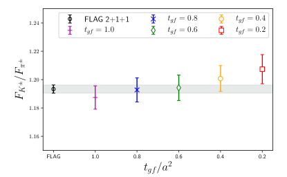
Figure 4: Flow-time (in)dependence of $F_{K^{\pm}}/F_{\pi^{\pm}}$ at the physical point $m_{\pi}\approx 135$ MeV in the continuum limit. The colored symbols are the results of our calculations extrapolated to the continuum limit and to the physical point using Eq. (VI.1). The benchmark FLAG result is the leftmost black point and it is consistent with our results at all flow-times within 1-sigma (horizontal gray band). The linear trend in flow-time observed is not present in the full continuum, chiral extrapolation analysis of different, but consistent, analysis of pseudoscalar correlation functions, so we believe this observed trend is not statistically significant.

VI.2 MA EFT extrapolation at $t_{gf}=1$

While the numerical results are sufficient to constrain the unknown LECs, we note that for larger flow-times the quality of the fit decreases, hinting at missing dependence upon the input parameters. For $t_{gf}=1$, we have also computed the mixed-meson masses, and so we can perform the full MA EFT extrapolation. The NLO MA EFT expressions for $f_{\pi}=\sqrt{2}F_{\pi}$ and $f_{K}$ are provided in Eqs. (C1) and (C2) of Ref. Chen et al. (2007), respectively. In our case, we have tuned the valence quark masses such that the pion mass matches the taste-5 HISQ pion mass, which implies ${\Delta}_{ju}={\Delta}_{rs}=0$ in the reference expressions. Further, the mixed-meson mass splitting is independent of quark mass at LO, allowing us to simplify the extrapolation formula. To simplify transcribing the expression, we define

$${\epsilon}_{\pi}^{2}=\frac{m_{\pi}^{2}}{{\Lambda}_{\chi}^{2}}, {\epsilon}_{ju}^{2}=\frac{m_{\pi}^{2}+a^{2}\tilde{{\Delta}}_{\textrm{Mix}}}{{\Lambda}_{\chi}^{2}},$$

$${\epsilon}_{K}^{2}=\frac{m_{K}^{2}}{{\Lambda}_{\chi}^{2}}, {\epsilon}_{ru}^{2}={\epsilon}_{sj}^{2}=\frac{m_{K}^{2}+a^{2}\tilde{{\Delta}}_{\textrm{Mix}}}{{\Lambda}_{\chi}^{2}},$$

$${\epsilon}_{ss}^{2}=\frac{m_{ss}^{2}}{{\Lambda}_{\chi}^{2}}, {\epsilon}_{rs}^{2}=\frac{m_{ss}^{2}+a^{2}\tilde{{\Delta}}_{\textrm{Mix}}}{{\Lambda}_{\chi}^{2}},$$

$${\delta}_{PQ}^{2}=\frac{a^{2}{\Delta}_{\rm I}}{{\Lambda}_{\chi}^{2}}, {\epsilon}_{X}^{2}=\frac{4}{3}{\epsilon}_{K}^{2}-\frac{1}{3}{\epsilon}_{\pi}^{2}+{\delta}_{PQ}^{2},$$

and $${\Lambda}_{\chi}^{2}=16\pi^{2}F_{\pi}F_{K}.$$ (16)

The resulting MA EFT expression is

$$\frac{F_{K}}{F_{\pi}} =1+\frac{1}{2}{\epsilon}_{ju}^{2}\ell_{ju}+\frac{1}{8}\ell_{\pi}\left\{{\epsilon}_{\pi}^{2}-\frac{{\delta}_{PQ}^{2}({\epsilon}_{X}^{2}+{\epsilon}_{\pi}^{2})}{{\epsilon}_{X}^{2}-{\epsilon}_{\pi}^{2}}\right.$$

$$\phantom{=}\left.+\frac{{\delta}_{PQ}^{4}{\epsilon}_{X}^{2}}{3({\epsilon}_{X}^{2}-{\epsilon}_{\pi}^{2})^{2}}-\frac{4{\delta}_{PQ}^{4}{\epsilon}_{\pi}^{2}}{3({\epsilon}_{X}^{2}-{\epsilon}_{\pi}^{2})({\epsilon}_{ss}^{2}-{\epsilon}_{\pi}^{2})}\right\}$$

$$\phantom{=}-\frac{1}{2}{\epsilon}_{sj}^{2}\ell_{sj}+\frac{1}{4}{\epsilon}_{ru}^{2}\ell_{ru}-\frac{1}{4}{\epsilon}_{rs}^{2}\ell_{rs}+\frac{\ell_{ss}}{4}\Bigg{\{}{\epsilon}_{ss}^{2}$$

$$\phantom{=}+\frac{{\delta}_{PQ}^{2}(3{\epsilon}_{ss}^{4}+2({\epsilon}_{K}^{2}-{\epsilon}_{\pi}^{2}){\epsilon}_{X}^{2}-3{\epsilon}_{ss}^{2}{\epsilon}_{X}^{2})}{3({\epsilon}_{X}^{2}-{\epsilon}_{ss}^{2})^{2}}$$

$$\phantom{=}\left.-\frac{{\delta}_{PQ}^{4}(2{\epsilon}_{ss}^{4}-{\epsilon}_{X}^{2}({\epsilon}_{ss}^{2}+{\epsilon}_{\pi}^{2}))}{3({\epsilon}_{X}^{2}-{\epsilon}_{ss}^{2})^{2}({\epsilon}_{ss}^{2}-{\epsilon}_{\pi}^{2})}\right\}-\frac{3}{8}{\epsilon}_{X}^{2}\ell_{X}\Bigg{\{}1$$

$$\phantom{=}-\frac{2{\delta}_{PQ}^{2}/3}{({\epsilon}_{X}^{2}-{\epsilon}_{\pi}^{2})}+\frac{{\delta}_{PQ}^{2}[4({\epsilon}_{K}^{2}-{\epsilon}_{\pi}^{2})+6({\epsilon}_{ss}^{2}-{\epsilon}_{X}^{2})]}{9({\epsilon}_{X}^{2}-{\epsilon}_{ss}^{2})^{2}}$$

$$\phantom{=}+\frac{{\delta}_{PQ}^{4}/9}{({\epsilon}_{X}^{2}-{\epsilon}_{\pi}^{2})^{2}}-\frac{2{\delta}_{PQ}^{4}(2{\epsilon}_{ss}^{2}-{\epsilon}_{\pi}^{2}-{\epsilon}_{X}^{2})}{9({\epsilon}_{X}^{2}-{\epsilon}_{ss}^{2})^{2}({\epsilon}_{X}^{2}-{\epsilon}_{\pi}^{2})}\Bigg{\}}$$

$$\phantom{=}+\frac{{\delta}_{PQ}^{2}({\epsilon}_{K}^{2}-{\epsilon}_{\pi}^{2})}{6({\epsilon}_{X}^{2}-{\epsilon}_{ss}^{2})}+\frac{{\delta}_{PQ}^{4}/24}{({\epsilon}_{X}^{2}-{\epsilon}_{\pi}^{2})}-\frac{{\delta}_{PQ}^{4}/12}{({\epsilon}_{X}^{2}-{\epsilon}_{ss}^{2})}$$

$$\phantom{=}-\frac{{\delta}_{PQ}^{2}}{8}+4({\epsilon}_{K}^{2}-{\epsilon}_{\pi}^{2})(4\pi)^{2}L_{5}({\Lambda}_{\chi})\,.$$ (17)

In this expression, we have only included the NLO counterterm, which is the same as in $SU(3)$ $\chi$PT, $L_{5}$. We observe that with this MA expression, the $a^{2}(m_{K}^{2}-m_{\pi}^{2})$ term is no longer needed to fit the data. When it is included, the fit returns a value of this LEC 2 orders of magnitude smaller than when using Eq. (VI.1). For this analysis, we have taken the values of $w_{0}^{2}{\Delta}m_{ju}^{2}$ from Table 4, combined with the values of $a/w_{0}$ from Ref. Bazavov et al. (2016a) to determine the values of $a^{2}\tilde{{\Delta}}_{\textrm{Mix}}$. We have used the values of $r_{1}^{2}a^{2}{\Delta}_{\rm I}$ and $r_{1}/a$ from Ref. Bazavov et al. (2013) to convert them to lattice units and combine them to form the necessary quantities in Eq. (VI.2). We observe that the MA expression is approximately 150 times more likely to reproduce the observed data when compared to $SU(3)$ $\chi$PT, as determined by the Bayes factors given in Table 5, providing very strong evidence that the MA expression provides the more correct physical point extrapolation. We leave further investigation of $F_{K}/F_{\pi}$ with more statistics and more ensembles to future work.

Table 5: Physical extrapolation from the $F_{K}/F_{\pi}$ analysis. The $Q$-value is the Bayesian analog of the $p$-value defined in Eq. (B4) of Ref. Bazavov et al. (2016b). The logGBF denotes the log of the Gaussian Bayes factor and is used to select models under the Bayesian framework. The Bayes factors are suppressed for $t_{gf}$ less than 1.0 since model comparisons are only sensible within the same data set.

$t_{gf}$	Function	$10^{3}\times L_{5}$	$F_{K}/F_{\pi}$	$Q$-value	logGBF
0.2	Eq. (VI.1)	5.55(1.17)	1.2102(105)	0.836	—
0.4	Eq. (VI.1)	4.79(1.03)	1.2034(93)	0.808	—
0.6	Eq. (VI.1)	4.05(1.02)	1.1968(92)	0.686	—
0.8	Eq. (VI.1)	3.88(96)	1.1952(87)	0.448	—
1.0	Eq. (VI.1)	3.27(93)	1.1898(84)	0.278	6.915
1.0	Eq. (VI.2)	3.35(33)	1.1905(32)	0.296	11.947

VII MDWF in QUDA: optimizations and performance

In order to efficiently perform the MDWF solves, we utilize the GPU implementation of the MDWF operator and solver Kim and Izubuchi (2014) from the highly optimized QUDA library Clark et al. (2010); Babich et al. (2011). We added the API for accessing this solver to the Chroma Edwards and Joo (2005) package, which is publicly available in the most recent version.

The MDWF calculations were performed on three different GPU-enabled machines, Surface and RZHasGPU at LLNL and Titan at OLCF. The Surface cluster is composed of dual NVIDIA Tesla K40 cards with Intel Xeon E5-2670 CPU nodes. The RZHasGPU cluster is composed of dual NVIDIA Tesla K80 cards with Intel Xeon E5-2667 v3 CPU nodes. The Titan supercomputer is composed of single NVIDIA Tesla K20X cards with AMD Opteron CPU nodes. An interesting feature of the Titan nodes is the use of two 8-core NUMA nodes per node. We have found that we can provide 2 MPI ranks per GPU, by using both NUMA nodes, and achieve an approximately 69% performance boost with otherwise identical parameters. In Table 6, we list the sustained performance on the three machines achieved with the present implementation of the double-half mixed-precision MDWF solver. The single node performance is notable, and we are at present working on improving the strong scaling of the MDWF solver in QUDA through better overlapping of communication and computation. Additionally, a significant reduction of the condition number for the symmetric implementation of the MDWF operator has been observed Blum et al. . QUDA supports both the symmetric and asymmetric implementations of the MDWF operator. Currently, Chroma only supports the asymmetric operator, but we plan to investigate possible reduction in the time to solution from switching to the symmetric implementation.

Table 6: Performance of the double-half mixed precision MDWF solver in QUDA on the various compute nodes used with 2, 4 and 1 GPU per node on the Surface, RZHasGPU and Titan computers. The % of peak performance is obtained by comparing our sustained to the theoretical single-node single-precision performance. On Titan, we oversubscribe the GPUs by using 1 MPI rank per NUMA node, which amounts to 2 MPI ranks per GPU, resulting in a $\sim 69\%$ performance boost.

Computer	GPUs	MPI	Geometry	Performance [GFlops]
		ranks		Total	per node	% peak
Surface	2	2	1 1 1 2	1250	1250	44%
RZHasGPU	4	4	1 1 1 4	1785	1785	48%
Titan	8	16	1 1 2 8	2885	0361	25%
Titan	16	32	1 2 2 8	4720	0295	20%
Titan	32	64	1 2 4 8	8500	0266	18%

VIII Conclusions

In this work, we have motivated a new mixed lattice QCD action: Möbius domain-wall valence fermions solved with the dynamical $N_{f}=2+1+1$ HISQ sea fermions after a gradient smearing algorithm is used to filter out UV modes of the gluons. To retain the correct continuum limit, the gradient flow-time is held fixed in lattice units, such that any dependence upon this new scale also vanishes in the continuum limit. We demonstrate the flow-time independence of the continuum limit by computing two sample quantities, $F_{K}/F_{\pi}$ and $m_{N}/F_{\pi}$. An extrapolation of $F_{K}/F_{\pi}$ to the continuum, infinite volume and physical pion and kaon mass point is consistent with the FLAG average of the $N_{f}=2+1+1$ LQCD results for all flow-times explored in this work.

For flow-time of $t_{gf}=1$, we estimate the total systematic error from different chiral and continuum fits to be smaller than our current statistical uncertainty. Of particular note, we also demonstrate that the gradient flow smearing highly suppresses sources of residual chiral symmetry breaking in the action for moderate values of the flow-time: the axial renormalization constant becomes effectively lattice spacing independent and close to 1 for all ensembles at a flow-time of $t_{gf}=1$; the residual chiral symmetry breaking, measured by the quantity $m_{res}$, is exponentially damped with increasing flow-time and less than 10% of the input light quark mass for all ensembles, including the physical quark-mass ensembles, with $t_{gf}=1$ and moderate values of $L_{5}$.

This action, coupled with the use of the highly optimized QUDA library, provides an economical method of performing LQCD calculations with an action that respects chiral symmetry to a high degree. The MILC Collaboration has a long history of making their configurations freely available to all interested parties. The breadth of parameters used in the generation of the HISQ ensembles allows users to fully control all LQCD systematics: notably the continuum, and infinite volume extrapolations, as well as a physical quark-mass interpolation.

We have plans to use this action for computing various quantities relevant to fundamental nuclear and high-energy physics research, detailed, for example, in the NSAC Long Range Plan for Nuclear Science and the HEPAP P5 Strategic Plan for U.S. Particle Physics. So far, we have used this mixed action to demonstrate the benefits of a new method for computing hadronic matrix elements Bouchard et al. (2017), applied this method to a precise determination of $g_{A}$ Berkowitz et al. (2017), and we have computed the $\pi^{-}\rightarrow\pi^{+}$ transition matrix elements relevant for the scenario in which heavy lepton-number violating physics beyond the Standard Model contributes to the hypothesized neutrinoless double beta decay of large nuclei Nicholson et al. (2016).

Appendix A Tables of flow-time dependence

Here, we provide tables of the various quantities computed in this work on the different flow-times used. Tuned quark masses and measured renormalization constants are reported in Table 7, while hadron masses and meson decay constants are summarized in Table 8.

Table 7: The tuned values of the MDWF light and strange quark masses on various ensembles for various flow-times. We also list the values of the average plaquette after applying the gradient flow as well as $m_{res}$ and the renormalization constants.

Ensemble	$M_{5}$	$L_{5}$	$b_{5}$	$c_{5}$	$t_{gf}$	Plaquette	$am_{l}^{mdwf}$	$am_{l}^{res}$	$Z_{A}^{ll}$	$am_{s}^{mdwf}$	$am_{s}^{res}$	$Z_{A}^{ls}$
a15m310	1.3	12	1.5	0.5	0.2	0.87701(2)	0.00970	0.003882(38)	0.8668(36)	0.06810	0.003022(31)	0.8740(13)
					0.4	0.95521(1)	0.01160	0.002290(29)	0.8993(34)	0.07380	0.001668(22)	0.9074(12)
					0.6	0.97723(1)	0.01250	0.001656(26)	0.9274(26)	0.08000	0.001163(19)	0.9389(12)
					0.8	0.98560(1)	0.01480	0.001287(24)	0.9498(24)	0.08520	0.000880(17)	0.9608(11)
					1.0	0.98964(1)	0.01580	0.001022(23)	0.9645(21)	0.09020	0.000685(15)	0.9760(09)
a12m310	1.2	8	1.25	0.25	0.2	0.89320(1)	0.00680	0.004298(22)	0.9007(23)	0.05300	0.003416(18)	0.9034(10)
					0.4	0.96401(1)	0.00960	0.001922(18)	0.9201(20)	0.05830	0.001352(15)	0.9243(07)
					0.6	0.98251(1)	0.01086	0.001332(17)	0.9418(18)	0.06280	0.000860(13)	0.9464(07)
					0.8	0.98925(0)	0.01176	0.001019(15)	0.9565(18)	0.06650	0.000615(11)	0.9608(07)
					1.0	0.99242(0)	0.01260	0.000804(14)	0.9660(17)	0.06930	0.000467(09)	0.9705(06)
a09m310	1.1	6	1.25	0.25	0.2	0.91073(0)	0.00543	0.002704(07)	0.9319(18)	0.03880	0.002359(05)	0.9343(05)
					0.4	0.97236(0)	0.00798	0.000616(05)	0.9444(16)	0.04330	0.000459(04)	0.9452(06)
					0.6	0.98721(0)	0.00850	0.000364(04)	0.9577(15)	0.04500	0.000251(03)	0.9590(05)
					0.8	0.99239(0)	0.00921	0.000280(04)	0.9659(13)	0.04780	0.000189(02)	0.9679(04)
					1.0	0.99478(0)	0.00951	0.000242(04)	0.9719(13)	0.04910	0.000169(02)	0.9739(04)
a15m220	1.3	16	1.75	0.75	0.2	0.87718(1)	0.00425	0.002254(18)	0.8634(38)	0.06810	0.001699(17)	0.8713(12)
					0.4	0.95535(1)	0.00532	0.001356(16)	0.8892(33)	0.07380	0.000953(14)	0.9064(12)
					0.6	0.97735(1)	0.00615	0.000966(14)	0.9221(31)	0.08000	0.000658(11)	0.9398(13)
					0.8	0.98570(1)	0.00668	0.000733(11)	0.9456(27)	0.08520	0.000492(10)	0.9617(11)
					1.0	0.98973(1)	0.00712	0.000567(10)	0.9610(26)	0.09020	0.000374(09)	0.9765(09)
a12m220	1.2	12	1.5	0.5	0.2	0.89332(1)	0.00365	0.001562(11)	0.8923(25)	0.05480	0.001085(10)	0.9026(21)
					0.4	0.96410(0)	0.00456	0.000935(09)	0.9132(22)	0.05880	0.000582(07)	0.9240(17)
					0.6	0.98259(0)	0.00522	0.000673(08)	0.9409(37)	0.06280	0.000391(06)	0.9466(14)
					0.8	0.98931(0)	0.00575	0.000511(07)	0.9546(28)	0.06660	0.000286(05)	0.9621(12)
					1.0	0.99248(0)	0.00600	0.000390(05)	0.9615(22)	0.06930	0.000216(04)	0.9718(11)

Table 8: Various hadronic quantities determined at different flow-times. The posterior distributions related to meson and baryon correlation functions are extracted using a $2+1$-state fit Ansatz for mesons and $2$ states for the nucleons, as described in Secs. IV.1 and IV.2. The meson two-point correlation functions are fit simultaneously with the 4D axial-vector current, and then a chained fit Bouchard et al. (2014) is used to propagate all remaining correlations. The entire fit strategy is implemented under the Bayesian framework with lsqfit Lepage (2016).

Ensemble	$t_{gf}$	$am_{\pi}$	$am_{K}$	$am_{ss}$	$aF_{\pi}$	$aF_{K}$	$am_{N}$	$F_{K}/F_{\pi}$	$m_{N}/F_{\pi}$
a15m310	0.2	0.2352(13)0	0.4025(12)	0.51904(87)	0.07781(85)	0.08724(85)	0.845(28)	1.1212(66)	10.86(38)
	0.4	0.2327(13)0	0.4014(12)	0.51710(89)	0.07720(69)	0.08572(64)	0.834(15)	1.1103(61)	10.80(22)
	0.6	0.2286(11)0	0.4004(12)	0.51673(91)	0.07599(54)	0.08439(53)	0.823(13)	1.1107(58)	10.84(19)
	0.8	0.2363(11)0	0.4028(12)	0.51673(92)	0.07543(53)	0.08343(49)	0.826(11)	1.1059(53)	10.95(17)
	1.0	0.2367(12)0	0.4046(12)	0.51858(94)	0.07436(51)	0.08239(46)	0.821(10)	1.1080(51)	11.05(16)
a12m310	0.2	0.18876(60)	0.3233(07)	0.41835(61)	0.06385(65)	0.07137(63)	0.673(32)	1.1177(57)	10.54(51)
	0.4	0.18842(62)	0.3233(07)	0.41773(60)	0.06306(53)	0.07008(47)	0.649(35)	1.1113(48)	10.29(56)
	0.6	0.18837(64)	0.3232(07)	0.41754(59)	0.06243(48)	0.06911(40)	0.641(34)	1.1070(46)	10.26(54)
	0.8	0.18833(65)	0.3234(07)	0.41776(58)	0.06196(44)	0.06832(36)	0.641(30)	1.1027(45)	10.35(49)
	1.0	0.18911(65)	0.3232(07)	0.41721(58)	0.06142(41)	0.06755(34)	0.642(27)	1.0999(44)	10.46(44)
a09m310	0.2	0.13982(42)	0.2411(04)	0.31227(36)	0.04578(45)	0.05174(47)	0.485(20)	1.1302(52)	10.60(45)
	0.4	0.14017(39)	0.2423(04)	0.31392(36)	0.04590(36)	0.05159(35)	0.489(18)	1.1239(46)	10.66(41)
	0.6	0.13860(38)	0.2396(04)	0.31041(37)	0.04568(33)	0.05113(31)	0.488(16)	1.1195(46)	10.69(37)
	0.8	0.14026(38)	0.2416(04)	0.31280(37)	0.04550(31)	0.05090(29)	0.488(14)	1.1186(45)	10.71(33)
	1.0	0.13978(38)	0.2405(04)	0.31129(38)	0.04521(30)	0.05047(28)	0.485(13)	1.1163(44)	10.72(31)
a15m220	0.2	0.16707(94)	0.3838(09)	0.51227(74)	0.07616(82)	0.08794(70)	0.788(37)	1.1546(74)	10.35(49)
	0.4	0.16668(82)	0.3848(09)	0.51195(72)	0.07521(74)	0.08638(58)	0.794(34)	1.1485(74)	10.56(47)
	0.6	0.16683(79)	0.3852(08)	0.51184(70)	0.07425(67)	0.08481(51)	0.787(18)	1.1422(72)	10.60(27)
	0.8	0.16647(76)	0.3853(09)	0.51195(70)	0.07343(63)	0.08338(45)	0.776(29)	1.1355(71)	10.57(41)
	1.0	0.16629(85)	0.3866(09)	0.51388(70)	0.07231(61)	0.08205(42)	0.766(28)	1.1348(72)	10.59(40)
a12m220	0.2	0.13305(58)	0.3080(12)	0.41732(56)	0.05732(63)	0.06618(84)	0.629(28)	1.154(12)0	10.97(50)
	0.4	0.13370(54)	0.3086(11)	0.41636(72)	0.05773(53)	0.06610(76)	0.581(48)	1.145(12)0	10.06(85)
	0.6	0.13354(96)	0.3088(10)	0.41583(55)	0.05784(51)	0.06582(63)	0.620(27)	1.138(10)0	10.73(48)
	0.8	0.13491(75)	0.3103(07)	0.41690(53)	0.05778(47)	0.06572(38)	0.621(23)	1.1374(69)	10.74(41)
	1.0	0.13424(66)	0.3097(07)	0.41618(52)	0.05731(45)	0.06514(35)	0.619(19)	1.1367(69)	10.80(36)

Appendix B Priors for correlator fits

In Table 9 we summarize the Bayesian priors used in the analysis of the mesonic two-point functions, together with the ones for the nucleon correlator and $m_{res}$. Notice that the priors are chosen to be independent of the gradient flow-time.

Table 9: Priors for correlator fits in lattice units. The priors are all Gaussian distributed and listed as mean(standard deviation). The oscillating and first excited-state energies are defined as splitting from the ground state, where $\Delta_{i}\equiv\ln(E_{i}-E_{0})$. This leads to a log-normal distributed energy splitting which is positive definite, and as a result enforces a strict hierarchy of states. The priors are chosen to be flow-time independent.

	$E_{0}^{\pi}$	$z_{0,p}^{\pi}$	$z_{0,s}^{\pi}$	$E_{0}^{K}$	$z_{0,p}^{K}$	$z_{0,s}^{K}$	$E_{0}^{ss}$	$z_{0,p}^{ss}$	$z_{0,s}^{ss}$
a15m310	0.2360(236)	0.255(255)	0.025(25)	0.4050(405)	0.198(198)	0.0198(198)	0.520(52)	0.182(182)	0.0185(185)
a12m310	0.190(19)	0.19(19)	0.02(2)	0.3220(322)	0.148(148)	0.0159(159)	0.4180(418)	0.142(142)	0.0152(152)
a09m310	0.140(14)	0.122(122)	0.0047(47)	0.2420(242)	0.1(1)	0.0039(39)	0.3120(312)	0.1(1)	0.0037(37)
a15m220	0.1660(166)	0.325(325)	0.031(31)	0.3850(385)	0.2(2)	0.02(2)	0.5150(515)	0.18(18)	0.0184(184)
a12m220	0.1340(134)	0.224(224)	0.0115(115)	0.310(31)	0.15(15)	0.0079(79)	0.4150(415)	0.137(137)	0.0073(73)
	$\Delta_{\textrm{osc.}}^{\pi}$	$z_{\textrm{osc.},p}^{\pi}$	$z_{\textrm{osc.},s}^{\pi}$	$\Delta_{\textrm{osc.}}^{K}$	$z_{\textrm{osc.},p}^{K}$	$z_{\textrm{osc.},s}^{K}$	$\Delta_{\textrm{osc.}}^{ss}$	$z_{\textrm{osc.},p}^{ss}$	$z_{\textrm{osc.},s}^{ss}$
a15m310	0(1.45)	0(0.255)	0(0.0125)	0(1.45)	0(0.198)	0(0.01)	0(1.45)	0(0.182)	0(0.009)
a12m310	0(1.67)	0(0.19)	0(0.01)	0(1.67)	0(0.148)	0(0.008)	0(1.67)	0(0.142)	0(0.008)
a09m310	0(1.96)	0(0.122)	0(0.00235)	0(1.96)	0(0.1)	0(0.0018)	0(1.96)	0(0.1)	0(0.0018)
a15m220	0(1.8)	0(0.325)	0(0.015)	0(1.8)	0(0.2)	0(0.01)	0(1.8)	0(0.18)	0(0.009)
a12m220	0(2)	0(0.224)	0(0.0057)	0(2)	0(0.15)	0(0.004)	0(2)	0(0.137)	0(0.004)
	$\Delta_{1}^{\pi}$	$z_{1,p}^{\pi}$	$z_{1,s}^{\pi}$	$\Delta_{1}^{K}$	$z_{1,p}^{K}$	$z_{1,s}^{K}$	$\Delta_{1}^{ss}$	$z_{1,p}^{ss}$	$z_{1,s}^{ss}$
a15m310	-0.75(70)	0(0.255)	0(0.0125)	-0.75(70)	0(0.198)	0(0.01)	-0.75(70)	0(0.182)	0(0.009)
a12m310	-0.97(70)	0(0.19)	0(0.01)	-0.97(70)	0(0.148)	0(0.008)	-0.97(70)	0(0.142)	0(0.008)
a09m310	-1.26(70)	0(0.122)	0(0.00235)	-1.26(70)	0(0.1)	0(0.0018)	-1.26(70)	0(0.1)	0(0.0018)
a15m220	-1.1(7)	0(0.325)	0(0.015)	-1.1(7)	0(0.2)	0(0.01)	-1.1(7)	0(0.18)	0(0.009)
a12m220	-1.3(7)	0(0.224)	0(0.0057)	-1.3(7)	0(0.15)	0(0.004)	-1.3(7)	0(0.137)	0(0.004)
	$f_{0}^{\pi}$	$f_{\textrm{osc.}}^{\pi}$	$f_{1}^{\pi}$	$f_{0}^{K}$	$f_{\textrm{osc.}}^{K}$	$f_{1}^{K}$	$f_{0}^{ss}$	$f_{\textrm{osc.}}^{ss}$	$f_{1}^{ss}$
a15m310	0.0387(387)	0(0.0387)	0(0.0387)	0.054(54)	0(0.054)	0(0.054)	0.0648(648)	0(0.0648)	0(0.0648)
a12m310	0.028(20)	0(0.028)	0(0.028)	0.04(4)	0(0.04)	0(0.04)	0.0485(485)	0(0.0485)	0(0.0485)
a09m310	0.0175(175)	0(0.0175)	0(0.0175)	0.0256(256)	0(0.0256)	0(0.0256)	0.0318(318)	0(0.0318)	0(0.0318)
a15m220	0.0309(309)	0(0.0309)	0(0.0309)	0.0522(522)	0(0.0522)	0(0.0522)	0.0636(636)	0(0.0636)	0(0.0636)
a12m220	0.0221(221)	0(0.0221)	0(0.0221)	0.0375(375)	0(0.0375)	0(0.0375)	0.047(47)	0(0.047)	0(0.047)
	$E^{N}_{0}$	$z_{0,p}^{N}$	$z_{0,s}^{N}$	${\Delta}^{N}_{1}$	$z_{1,p}^{N}$	$z_{1,s}^{N}$	$m_{res}^{l}$	$m_{res}^{s}$
a15m310	0.820(82)	0.0112(55)	4.1(4.1)E-4	-0.75(70)	0(0.112)	0(0.0021)	0(1)	0(1)
a12m310	0.670(67)	0.006(3)	2.6(2.6)E-4	-1.0(7)	0(0.06)	0(0.0013)	0(1)	0(1)
a09m310	0.50(5)	0.0024(12)	2.2(2.2)E-5	-1.27(68)	0(0.024)	0(1.1)E-4	0(1)	0(1)
a15m220	0.760(76)	0.011(5)	4.2(4.2)E-4	-1.1(7)	0(0.11)	0(0.0021)	0(1)	0(1)
a12m220	0.610(61)	0.0054(27)	7.9(7.0)E-5	-1.3(7)	0(0.054)	0(4)E-4	0(1)	0(1)

Appendix C Correlator analysis fit regions

A summary of the fit regions for the two-point function analysis is shown in Table 10 for the three different ensembles used in this work. $q_{1}q_{2}$ superscripts identify mesonic states ($\pi$, $\bar{s}{\gamma}_{5}s$, and $K$.)

Table 10: Fit range in lattice units. The fit region is chosen to be approximately the same in physical units for all pseudoscalar correlator fits, as well as among the nucleon correlator fits. The nucleon correlation functions are fit closer to the origin because of the poorer signal-to-noise ratio as compared to pseudoscalar observables.

$a$	$C^{q_{1}q_{2}}$ t${}_{\textrm{min}}$	$C^{q_{1}q_{2}}$ t${}_{\textrm{max}}$	$C^{N}$ t${}_{\textrm{min}}$	$C^{N}$ t${}_{\textrm{max}}$
0.15 fm	7	15	4	10
0.12 fm	8	19	5	12
0.09 fm	12	25	7	16

Appendix D Topological charge evolution on HISQ ensembles

In this Appendix, we provide additional details for the $N_{f}=2+1+1$ HISQ ensembles at heavy pion masses ($m_{\pi}\approx$ 350 and 400 MeV). The ensembles have a lattice spacing of $\approx 0.12$ fm, and we expect the topological charge to fluctuate along the molecular dynamics trajectory and be Gaussian distributed. This behavior is plotted in Fig. 5 for both ensembles. Each of the new ensembles is obtained by combining configurations from eight independent streams (collected after each stream has thermalized), and they are plotted together in Fig. 5. We solve the gradient flow equations with the Symanzik action to smooth out the HISQ gauge fields, with a step size of $\epsilon=0.03$ and up to $n=166$ iterations. We use the symmetric Clover discretization of the bosonic topological charge density operator $G_{\mu\nu}\tilde{G}_{\mu\nu}$.

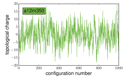
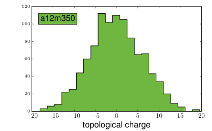
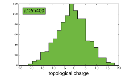
Figure 5: Topological charge of the a12m350 and a12m400 ensembles at flow-time $t_{gf}=0.99$. The topological charge randomly fluctuates and shows no long correlation as a function of configuration number (Monte Carlo time) for both ensembles. The histograms show that the fluctuations are centered around zero, indicating the absence of CP (charge-parity) violation, and are Gaussian distributed, indicating that the volumes are sufficiently large.

References

- Fritzsch and Gell-Mann (1972) Harald Fritzsch and Murray Gell-Mann, “Current algebra: Quarks and what else?” Proceedings, 16th International Conference on High-Energy Physics, ICHEP, Batavia, Illinois, 6-13 Sep 1972, eConf C720906V2, 135–165 (1972), arXiv:hep-ph/0208010 [hep-ph] .
- Fritzsch et al. (1973) H. Fritzsch, Murray Gell-Mann, and H. Leutwyler, “Advantages of the Color Octet Gluon Picture,” Phys. Lett. B47, 365–368 (1973).
- Gross and Wilczek (1973) David J. Gross and Frank Wilczek, “Ultraviolet Behavior of Nonabelian Gauge Theories,” Phys. Rev. Lett. 30, 1343–1346 (1973).
- Politzer (1973) H. David Politzer, “Reliable Perturbative Results for Strong Interactions?” Phys. Rev. Lett. 30, 1346–1349 (1973).
- Weinberg (1979) Steven Weinberg, “Phenomenological Lagrangians,” Physica A96, 327–340 (1979).
- Symanzik (1983a) K. Symanzik, “Continuum Limit and Improved Action in Lattice Theories. 1. Principles and phi**4 Theory,” Nucl. Phys. B226, 187–204 (1983a).
- Symanzik (1983b) K. Symanzik, “Continuum Limit and Improved Action in Lattice Theories. 2. O(N) Nonlinear Sigma Model in Perturbation Theory,” Nucl. Phys. B226, 205–227 (1983b).
- Aoki et al. (2017) S. Aoki et al., “Review of lattice results concerning low-energy particle physics,” Eur. Phys. J. C77, 112 (2017), arXiv:1607.00299 [hep-lat] .
- Wilson (1974) Kenneth G. Wilson, “Confinement of Quarks,” Phys. Rev. D10, 2445–2459 (1974).
- Sheikholeslami and Wohlert (1985) B. Sheikholeslami and R. Wohlert, “Improved Continuum Limit Lattice Action for QCD with Wilson Fermions,” Nucl. Phys. B259, 572 (1985).
- Frezzotti et al. (2001) Roberto Frezzotti, Pietro Antonio Grassi, Stefan Sint, and Peter Weisz (Alpha), “Lattice QCD with a chirally twisted mass term,” JHEP 08, 058 (2001), arXiv:hep-lat/0101001 [hep-lat] .
- Frezzotti and Rossi (2004) R. Frezzotti and G. C. Rossi, “Chirally improving Wilson fermions. 1. O(a) improvement,” JHEP 08, 007 (2004), arXiv:hep-lat/0306014 [hep-lat] .
- Kogut and Susskind (1975) John B. Kogut and Leonard Susskind, “Hamiltonian Formulation of Wilson’s Lattice Gauge Theories,” Phys. Rev. D11, 395–408 (1975).
- Susskind (1977) Leonard Susskind, “Lattice Fermions,” Phys. Rev. D16, 3031–3039 (1977).
- Marinari et al. (1981) E. Marinari, G. Parisi, and C. Rebbi, “Monte Carlo Simulation of the Massive Schwinger Model,” Nucl. Phys. B190, 734 (1981), [,595(1981)].
- Bernard et al. (2007) Claude Bernard, Maarten Golterman, Yigal Shamir, and Stephen R. Sharpe, “Comment on ‘Chiral anomalies and rooted staggered fermions’,” Phys. Lett. B649, 235–240 (2007), arXiv:hep-lat/0603027 [hep-lat] .
- Bernard et al. (2006) Claude Bernard, Maarten Golterman, and Yigal Shamir, “Observations on staggered fermions at non-zero lattice spacing,” Phys. Rev. D73, 114511 (2006), arXiv:hep-lat/0604017 [hep-lat] .
- Creutz (2007) Michael Creutz, “Chiral anomalies and rooted staggered fermions,” Phys. Lett. B649, 230–234 (2007), arXiv:hep-lat/0701018 [hep-lat] .
- Bernard (2005) C. Bernard, “Order of the chiral and continuum limits in staggered chiral perturbation theory,” Phys. Rev. D71, 094020 (2005), arXiv:hep-lat/0412030 [hep-lat] .
- Bernard (2006) C. Bernard, “Staggered chiral perturbation theory and the fourth-root trick,” Phys. Rev. D73, 114503 (2006), arXiv:hep-lat/0603011 [hep-lat] .
- Shamir (2005) Yigal Shamir, “Locality of the fourth root of the staggered-fermion determinant: Renormalization-group approach,” Phys. Rev. D71, 034509 (2005), arXiv:hep-lat/0412014 [hep-lat] .
- Shamir (2007) Yigal Shamir, “Renormalization-group analysis of the validity of staggered-fermion QCD with the fourth-root recipe,” Phys. Rev. D75, 054503 (2007), arXiv:hep-lat/0607007 [hep-lat] .
- Bernard et al. (2008a) Claude Bernard, Maarten Golterman, and Yigal Shamir, “Effective field theories for QCD with rooted staggered fermions,” Phys. Rev. D77, 074505 (2008a), arXiv:0712.2560 [hep-lat] .
- Durr and Hoelbling (2005) Stephan Durr and Christian Hoelbling, “Scaling tests with dynamical overlap and rooted staggered fermions,” Phys. Rev. D71, 054501 (2005), arXiv:hep-lat/0411022 [hep-lat] .
- Durr and Hoelbling (2006) Stephan Durr and Christian Hoelbling, “Lattice fermions with complex mass,” Phys. Rev. D74, 014513 (2006), arXiv:hep-lat/0604005 [hep-lat] .
- Hasenfratz and Hoffmann (2006) Anna Hasenfratz and Roland Hoffmann, “Validity of the rooted staggered determinant in the continuum limit,” Phys. Rev. D74, 014511 (2006), arXiv:hep-lat/0604010 [hep-lat] .
- Bernard et al. (2008b) Claude Bernard, Maarten Golterman, Yigal Shamir, and Stephen R. Sharpe, “’t Hooft vertices, partial quenching, and rooted staggered QCD,” Phys. Rev. D77, 114504 (2008b), arXiv:0711.0696 [hep-lat] .
- Sharpe (2006) Stephen R. Sharpe, “Rooted staggered fermions: Good, bad or ugly?” Proceedings, 24th International Symposium on Lattice Field Theory (Lattice 2006): Tucson, USA, July 23-28, 2006, PoS LAT2006, 022 (2006), arXiv:hep-lat/0610094 [hep-lat] .
- Kronfeld (2007) Andreas S. Kronfeld, “Lattice Gauge Theory with Staggered Fermions: How, Where, and Why (Not),” Proceedings, 25th International Symposium on Lattice field theory (Lattice 2007): Regensburg, Germany, July 30-August 4, 2007, PoS LAT2007, 016 (2007), arXiv:0711.0699 [hep-lat] .
- Bazavov et al. (2010a) A. Bazavov et al. (MILC), “Nonperturbative QCD Simulations with 2+1 Flavors of Improved Staggered Quarks,” Rev. Mod. Phys. 82, 1349–1417 (2010a), arXiv:0903.3598 [hep-lat] .
- Nielsen and Ninomiya (1981a) Holger Bech Nielsen and M. Ninomiya, “Absence of Neutrinos on a Lattice. 1. Proof by Homotopy Theory,” Nucl. Phys. B185, 20 (1981a), [,533(1980)].
- Nielsen and Ninomiya (1981b) Holger Bech Nielsen and M. Ninomiya, “Absence of Neutrinos on a Lattice. 2. Intuitive Topological Proof,” Nucl. Phys. B193, 173–194 (1981b).
- Nielsen and Ninomiya (1981c) Holger Bech Nielsen and M. Ninomiya, “No Go Theorem for Regularizing Chiral Fermions,” Phys. Lett. B105, 219–223 (1981c).
- Ginsparg and Wilson (1982) Paul H. Ginsparg and Kenneth G. Wilson, “A Remnant of Chiral Symmetry on the Lattice,” Phys. Rev. D25, 2649 (1982).
- Lüscher (1998) Martin Lüscher, “Exact chiral symmetry on the lattice and the Ginsparg-Wilson relation,” Phys. Lett. B428, 342–345 (1998), arXiv:hep-lat/9802011 [hep-lat] .
- Kaplan (1992) David B. Kaplan, “A Method for simulating chiral fermions on the lattice,” Phys. Lett. B288, 342–347 (1992), arXiv:hep-lat/9206013 [hep-lat] .
- Shamir (1993) Yigal Shamir, “Chiral fermions from lattice boundaries,” Nucl. Phys. B406, 90–106 (1993), arXiv:hep-lat/9303005 [hep-lat] .
- Furman and Shamir (1995) Vadim Furman and Yigal Shamir, “Axial symmetries in lattice QCD with Kaplan fermions,” Nucl. Phys. B439, 54–78 (1995), arXiv:hep-lat/9405004 [hep-lat] .
- Narayanan and Neuberger (1994) Rajamani Narayanan and Herbert Neuberger, “Chiral determinant as an overlap of two vacua,” Nucl. Phys. B412, 574–606 (1994), arXiv:hep-lat/9307006 [hep-lat] .
- Narayanan and Neuberger (1993) Rajamani Narayanan and Herbert Neuberger, “Chiral fermions on the lattice,” Phys. Rev. Lett. 71, 3251 (1993), arXiv:hep-lat/9308011 [hep-lat] .
- Narayanan and Neuberger (1995) Rajamani Narayanan and Herbert Neuberger, “A Construction of lattice chiral gauge theories,” Nucl. Phys. B443, 305–385 (1995), arXiv:hep-th/9411108 [hep-th] .
- Borici (2000) A. Borici, “Truncated overlap fermions,” Lattice field theory. Proceedings, 17th International Symposium, Lattice’99, Pisa, Italy, June 29-July 3, 1999, Nucl. Phys. Proc. Suppl. 83, 771–773 (2000), arXiv:hep-lat/9909057 [hep-lat] .
- Borici (1999) Artan Borici, “Truncated overlap fermions: The Link between overlap and domain wall fermions,” in Lattice fermions and structure of the vacuum. Proceedings, NATO Advanced Research Workshop, Dubna, Russia, October 5-9, 1999 (1999) pp. 41–52, arXiv:hep-lat/9912040 [hep-lat] .
- Kennedy (2005) A. D. Kennedy, “Algorithms for lattice QCD with dynamical fermions,” Lattice field theory. Proceedings, 22nd International Symposium, Lattice 2004, Batavia, USA, June 21-26, 2004, Nucl. Phys. Proc. Suppl. 140, 190–203 (2005), [,190(2004)], arXiv:hep-lat/0409167 [hep-lat] .
- Bar et al. (2003) Oliver Bar, Gautam Rupak, and Noam Shoresh, “Simulations with different lattice Dirac operators for valence and sea quarks,” Phys. Rev. D67, 114505 (2003), arXiv:hep-lat/0210050 [hep-lat] .
- Renner et al. (2005) Dru Bryant Renner, W. Schroers, R. Edwards, George Tamminga Fleming, Ph. Hagler, John W. Negele, K. Orginos, A. V. Pochinski, and D. Richards (LHP), “Hadronic physics with domain-wall valence and improved staggered sea quarks,” Lattice field theory. Proceedings, 22nd International Symposium, Lattice 2004, Batavia, USA, June 21-26, 2004, Nucl. Phys. Proc. Suppl. 140, 255–260 (2005), [,255(2004)], arXiv:hep-lat/0409130 [hep-lat] .
- Orginos and Toussaint (1999) Kostas Orginos and Doug Toussaint (MILC), “Testing improved actions for dynamical Kogut-Susskind quarks,” Phys. Rev. D59, 014501 (1999), arXiv:hep-lat/9805009 [hep-lat] .
- Orginos et al. (1999) Kostas Orginos, Doug Toussaint, and R. L. Sugar (MILC), “Variants of fattening and flavor symmetry restoration,” Phys. Rev. D60, 054503 (1999), arXiv:hep-lat/9903032 [hep-lat] .
- Bernard et al. (2001) Claude W. Bernard, Tom Burch, Kostas Orginos, Doug Toussaint, Thomas A. DeGrand, Carleton E. Detar, Saumen Datta, Steven A. Gottlieb, Urs M. Heller, and Robert Sugar, “The QCD spectrum with three quark flavors,” Phys. Rev. D64, 054506 (2001), arXiv:hep-lat/0104002 [hep-lat] .
- Edwards et al. (2006) R. G. Edwards, G. T. Fleming, Ph. Hagler, J. W. Negele, K. Orginos, A. V. Pochinsky, D. B. Renner, D. G. Richards, and W. Schroers (LHPC), “The Nucleon axial charge in full lattice QCD,” Phys. Rev. Lett. 96, 052001 (2006), arXiv:hep-lat/0510062 [hep-lat] .
- Hagler et al. (2008) Ph. Hagler et al. (LHPC), “Nucleon Generalized Parton Distributions from Full Lattice QCD,” Phys. Rev. D77, 094502 (2008), arXiv:0705.4295 [hep-lat] .
- Bratt et al. (2010) J. D. Bratt et al. (LHPC), “Nucleon structure from mixed action calculations using 2+1 flavors of asqtad sea and domain wall valence fermions,” Phys. Rev. D82, 094502 (2010), arXiv:1001.3620 [hep-lat] .
- Beane et al. (2006) S. R. Beane, P. F. Bedaque, K. Orginos, and M. J. Savage (NPLQCD), “Nucleon nucleon scattering from fully-dynamical lattice QCD,” Phys. Rev. Lett. 97, 012001 (2006), arXiv:hep-lat/0602010 .
- Beane et al. (2008) Silas R. Beane et al. (NPLQCD), “Precise Determination of the I=2 pipi Scattering Length from Mixed-Action Lattice QCD,” Phys. Rev. D77, 014505 (2008), arXiv:0706.3026 [hep-lat] .
- Walker-Loud et al. (2009) A. Walker-Loud et al., “Light hadron spectroscopy using domain wall valence quarks on an Asqtad sea,” Phys. Rev. D79, 054502 (2009), arXiv:0806.4549 [hep-lat] .
- Aubin et al. (2010) C. Aubin, Jack Laiho, and Ruth S. Van de Water, “The Neutral kaon mixing parameter B(K) from unquenched mixed-action lattice QCD,” Phys. Rev. D81, 014507 (2010), arXiv:0905.3947 [hep-lat] .
- Langacker and Pagels (1973) Paul Langacker and Heinz Pagels, “Chiral perturbation theory,” Phys. Rev. D8, 4595–4619 (1973).
- Gasser and Leutwyler (1984) J. Gasser and H. Leutwyler, “Chiral Perturbation Theory to One Loop,” Annals Phys. 158, 142 (1984).
- Leutwyler (1994) H. Leutwyler, “On the foundations of chiral perturbation theory,” Annals Phys. 235, 165–203 (1994), arXiv:hep-ph/9311274 [hep-ph] .
- Sharpe and Singleton (1998) Stephen R. Sharpe and Robert L. Singleton, Jr, “Spontaneous flavor and parity breaking with Wilson fermions,” Phys. Rev. D58, 074501 (1998), arXiv:hep-lat/9804028 [hep-lat] .
- Bar et al. (2004) Oliver Bar, Gautam Rupak, and Noam Shoresh, “Chiral perturbation theory at O(a**2) for lattice QCD,” Phys. Rev. D70, 034508 (2004), arXiv:hep-lat/0306021 [hep-lat] .
- Bar et al. (2005) Oliver Bar, Claude Bernard, Gautam Rupak, and Noam Shoresh, “Chiral perturbation theory for staggered sea quarks and Ginsparg-Wilson valence quarks,” Phys. Rev. D72, 054502 (2005), arXiv:hep-lat/0503009 [hep-lat] .
- Tiburzi (2005a) Brian C. Tiburzi, “Baryons with Ginsparg-Wilson quarks in a staggered sea,” Phys. Rev. D72, 094501 (2005a), [Erratum: Phys. Rev.D79,039904(2009)], arXiv:hep-lat/0508019 [hep-lat] .
- Chen et al. (2006) Jiunn-Wei Chen, Donal O’Connell, Ruth S. Van de Water, and Andre Walker-Loud, “Ginsparg-Wilson pions scattering on a staggered sea,” Phys. Rev. D73, 074510 (2006), arXiv:hep-lat/0510024 [hep-lat] .
- Chen et al. (2007) Jiunn-Wei Chen, Donal O’Connell, and Andre Walker-Loud, “Two Meson Systems with Ginsparg-Wilson Valence Quarks,” Phys. Rev. D75, 054501 (2007), arXiv:hep-lat/0611003 [hep-lat] .
- Orginos and Walker-Loud (2008) Kostas Orginos and Andre Walker-Loud, “Mixed meson masses with domain-wall valence and staggered sea fermions,” Phys. Rev. D77, 094505 (2008), arXiv:0705.0572 [hep-lat] .
- Jiang (2007) Fu-Jiun Jiang, “Mixed Action Lattice Spacing Effects on the Nucleon Axial Charge,” (2007), arXiv:hep-lat/0703012 [hep-lat] .
- Chen et al. (2009a) Jiunn-Wei Chen, Donal O’Connell, and Andre Walker-Loud, “Universality of mixed action extrapolation formulae,” JHEP 04, 090 (2009a), arXiv:0706.0035 [hep-lat] .
- Chen et al. (2009b) Jiunn-Wei Chen, Maarten Golterman, Donal O’Connell, and Andre Walker-Loud, “Mixed Action Effective Field Theory: An Addendum,” Phys. Rev. D79, 117502 (2009b), arXiv:0905.2566 [hep-lat] .
- Bernard and Golterman (1994) Claude W. Bernard and Maarten F. L. Golterman, “Partially quenched gauge theories and an application to staggered fermions,” Phys. Rev. D49, 486–494 (1994), arXiv:hep-lat/9306005 [hep-lat] .
- Sharpe and Shoresh (2000) Stephen R. Sharpe and Noam Shoresh, “Physical results from unphysical simulations,” Phys. Rev. D62, 094503 (2000), arXiv:hep-lat/0006017 [hep-lat] .
- Sharpe and Shoresh (2001) Stephen R. Sharpe and Noam Shoresh, “Partially quenched chiral perturbation theory without Phi0,” Phys. Rev. D64, 114510 (2001), arXiv:hep-lat/0108003 [hep-lat] .
- Chen and Savage (2002) Jiunn-Wei Chen and Martin J. Savage, “Baryons in partially quenched chiral perturbation theory,” Phys. Rev. D65, 094001 (2002), arXiv:hep-lat/0111050 [hep-lat] .
- Sharpe and Van de Water (2004) Stephen R. Sharpe and Ruth S. Van de Water, “Unphysical operators in partially quenched QCD,” Phys. Rev. D69, 054027 (2004), arXiv:hep-lat/0310012 [hep-lat] .
- Arndt and Tiburzi (2003a) Daniel Arndt and Brian C. Tiburzi, “Charge radii of the meson and baryon octets in quenched and partially quenched chiral perturbation theory,” Phys. Rev. D68, 094501 (2003a), arXiv:hep-lat/0307003 [hep-lat] .
- Walker-Loud (2005) Andre Walker-Loud, “Octet baryon masses in partially quenched chiral perturbation theory,” Nucl. Phys. A747, 476–507 (2005), arXiv:hep-lat/0405007 [hep-lat] .
- Bernard and Golterman (2010) Claude Bernard and Maarten Golterman, “Transfer Matrix for Partially Quenched QCD,” Proceedings, 28th International Symposium on Lattice field theory (Lattice 2010): Villasimius, Italy, June 14-19, 2010, PoS LATTICE2010, 252 (2010), arXiv:1011.0184 [hep-lat] .
- Bernard and Golterman (2013) Claude Bernard and Maarten Golterman, “On the foundations of partially quenched chiral perturbation theory,” Phys. Rev. D88, 014004 (2013), arXiv:1304.1948 [hep-lat] .
- Beane and Savage (2002) Silas R. Beane and Martin J. Savage, “Nucleons in two flavor partially quenched chiral perturbation theory,” Nucl. Phys. A709, 319–344 (2002), arXiv:hep-lat/0203003 [hep-lat] .
- Beane and Savage (2003) Silas R. Beane and Martin J. Savage, “Partially quenched nucleon nucleon scattering,” Phys. Rev. D67, 054502 (2003), arXiv:hep-lat/0210046 [hep-lat] .
- Arndt and Tiburzi (2003b) Daniel Arndt and Brian C Tiburzi, “Electromagnetic properties of the baryon decuplet in quenched and partially quenched chiral perturbation theory,” Phys. Rev. D68, 114503 (2003b), [Erratum: Phys. Rev.D69,059904(2004)], arXiv:hep-lat/0308001 [hep-lat] .
- Arndt and Tiburzi (2004) Daniel Arndt and Brian C. Tiburzi, “Baryon decuplet to octet electromagnetic transitions in quenched and partially quenched chiral perturbation theory,” Phys. Rev. D69, 014501 (2004), arXiv:hep-lat/0309013 [hep-lat] .
- Tiburzi and Walker-Loud (2005) Brian C. Tiburzi and Andre Walker-Loud, “Decuplet baryon masses in partially quenched chiral perturbation theory,” Nucl. Phys. A748, 513–536 (2005), arXiv:hep-lat/0407030 [hep-lat] .
- Tiburzi (2005b) Brian C. Tiburzi, “Baryon masses in partially quenched heavy hadron chiral perturbation theory,” Phys. Rev. D71, 034501 (2005b), arXiv:hep-lat/0410033 [hep-lat] .
- Tiburzi and Walker-Loud (2006) Brian C. Tiburzi and Andre Walker-Loud, “Strong isospin breaking in the nucleon and Delta masses,” Nucl. Phys. A764, 274–302 (2006), arXiv:hep-lat/0501018 [hep-lat] .
- O’Connell and Savage (2006) Donal O’Connell and Martin J. Savage, “Extrapolation formulas for neutron EDM calculations in lattice QCD,” Phys. Lett. B633, 319–324 (2006), arXiv:hep-lat/0508009 [hep-lat] .
- Prelovsek (2006) Sasa Prelovsek, “Effects of staggered fermions and mixed actions on the scalar correlator,” Phys. Rev. D73, 014506 (2006), arXiv:hep-lat/0510080 [hep-lat] .
- Aubin et al. (2008) C. Aubin, Jack Laiho, and Ruth S. Van de Water, “Discretization effects and the scalar meson correlator in mixed-action lattice simulations,” Phys. Rev. D77, 114501 (2008), arXiv:0803.0129 [hep-lat] .
- Na et al. (2015) Heechang Na, Chris M. Bouchard, G. Peter Lepage, Chris Monahan, and Junko Shigemitsu (HPQCD), “ form factors at nonzero recoil and extraction of ,” Phys. Rev. D92, 054510 (2015), [Erratum: Phys. Rev.D93,no.11,119906(2016)], arXiv:1505.03925 [hep-lat] .
- Donald et al. (2014) G. C. Donald, C. T. H. Davies, J. Koponen, and G. P. Lepage, “Prediction of the width from a calculation of its radiative decay in full lattice QCD,” Phys. Rev. Lett. 112, 212002 (2014), arXiv:1312.5264 [hep-lat] .
- Li et al. (2010) A. Li et al. (xQCD), “Overlap Valence on 2+1 Flavor Domain Wall Fermion Configurations with Deflation and Low-mode Substitution,” Phys. Rev. D82, 114501 (2010), arXiv:1005.5424 [hep-lat] .
- Lujan et al. (2012) M. Lujan, A. Alexandru, Y. Chen, T. Draper, W. Freeman, M. Gong, F. X. Lee, A. Li, K. F. Liu, and N. Mathur, “The parameter in the overlap on domain-wall mixed action,” Phys. Rev. D86, 014501 (2012), arXiv:1204.6256 [hep-lat] .
- Gong et al. (2013) M. Gong et al. (XQCD), “Strangeness and charmness content of the nucleon from overlap fermions on 2+1-flavor domain-wall fermion configurations,” Phys. Rev. D88, 014503 (2013), arXiv:1304.1194 [hep-ph] .
- Allton et al. (2007) C. Allton et al. (RBC, UKQCD), “2+1 flavor domain wall QCD on a (2 fm)*83 lattice: Light meson spectroscopy with L(s) = 16,” Phys. Rev. D76, 014504 (2007), arXiv:hep-lat/0701013 [hep-lat] .
- Aoki et al. (2011) Y. Aoki et al. (RBC, UKQCD), “Continuum Limit Physics from 2+1 Flavor Domain Wall QCD,” Phys. Rev. D83, 074508 (2011), arXiv:1011.0892 [hep-lat] .
- Basak et al. (2012) S. Basak, S. Datta, M. Padmanath, P. Majumdar, and N. Mathur, “Charm and strange hadron spectra from overlap fermions on HISQ gauge configurations,” Proceedings, 30th International Symposium on Lattice Field Theory (Lattice 2012): Cairns, Australia, June 24-29, 2012, PoS LATTICE2012, 141 (2012), arXiv:1211.6277 [hep-lat] .
- Basak et al. (2014) S. Basak, S. Datta, A. T. Lytle, M. Padmanath, P. Majumdar, and N. Mathur, “Hadron spectra from overlap fermions on HISQ gauge configurations,” Proceedings, 31st International Symposium on Lattice Field Theory (Lattice 2013): Mainz, Germany, July 29-August 3, 2013, PoS LATTICE2013, 243 (2014), arXiv:1312.3050 [hep-lat] .
- Basak et al. (2015) S. Basak, S. Datta, Nilmani Mathur, A. T. Lytle, Pushan Majumdar, and M. Padmanath (ILGTI), “Hadron spectra and from overlap quarks on a HISQ sea,” Proceedings, 32nd International Symposium on Lattice Field Theory (Lattice 2014): Brookhaven, NY, USA, June 23-28, 2014, PoS LATTICE2014, 083 (2015), arXiv:1412.7248 [hep-lat] .
- Mathur et al. (2016) Nilmani Mathur, M. Padmanath, and Randy Lewis, “Charmed-Bottom Mesons from Lattice QCD,” Proceedings, 34th International Symposium on Lattice Field Theory (Lattice 2016): Southampton, UK, July 24-30, 2016, PoS LATTICE2016, 100 (2016), arXiv:1611.04085 [hep-lat] .
- Bhattacharya et al. (2014) Tanmoy Bhattacharya, Saul D. Cohen, Rajan Gupta, Anosh Joseph, Huey-Wen Lin, and Boram Yoon, “Nucleon Charges and Electromagnetic Form Factors from 2+1+1-Flavor Lattice QCD,” Phys. Rev. D89, 094502 (2014), arXiv:1306.5435 [hep-lat] .
- Bhattacharya et al. (2015) Tanmoy Bhattacharya, Vincenzo Cirigliano, Saul Cohen, Rajan Gupta, Anosh Joseph, Huey-Wen Lin, and Boram Yoon (PNDME), “Iso-vector and Iso-scalar Tensor Charges of the Nucleon from Lattice QCD,” Phys. Rev. D92, 094511 (2015), arXiv:1506.06411 [hep-lat] .
- Durr et al. (2012) S. Durr et al., “Sigma term and strangeness content of octet baryons,” Phys. Rev. D85, 014509 (2012), [Erratum: Phys. Rev.D93,no.3,039905(2016)], arXiv:1109.4265 [hep-lat] .
- Durr et al. (2016) S. Durr et al., “Lattice computation of the nucleon scalar quark contents at the physical point,” Phys. Rev. Lett. 116, 172001 (2016), arXiv:1510.08013 [hep-lat] .
- Yang et al. (2016) Yi-Bo Yang, Andrei Alexandru, Terrence Draper, Jian Liang, and Keh-Fei Liu (xQCD), “N and strangeness sigma terms at the physical point with chiral fermions,” Phys. Rev. D94, 054503 (2016), arXiv:1511.09089 [hep-lat] .
- Sufian et al. (2017) Raza Sabbir Sufian, Yi-Bo Yang, Andrei Alexandru, Terrence Draper, Jian Liang, and Keh-Fei Liu, “Strange Quark Magnetic Moment of the Nucleon at the Physical Point,” Phys. Rev. Lett. 118, 042001 (2017), arXiv:1606.07075 [hep-ph] .
- Bhattacharya et al. (2016) Tanmoy Bhattacharya, Vincenzo Cirigliano, Saul Cohen, Rajan Gupta, Huey-Wen Lin, and Boram Yoon, “Axial, Scalar and Tensor Charges of the Nucleon from 2+1+1-flavor Lattice QCD,” Phys. Rev. D94, 054508 (2016), arXiv:1606.07049 [hep-lat] .
- Borsanyi et al. (2013) Sz. Borsanyi et al. (Budapest-Marseille-Wuppertal), “Isospin splittings in the light baryon octet from lattice QCD and QED,” Phys. Rev. Lett. 111, 252001 (2013), arXiv:1306.2287 [hep-lat] .
- Borsanyi et al. (2015) Sz. Borsanyi et al., “Ab initio calculation of the neutron-proton mass difference,” Science 347, 1452–1455 (2015), arXiv:1406.4088 [hep-lat] .
- Brantley et al. (2016) David A. Brantley, Balint Joo, Ekaterina V. Mastropas, Emanuele Mereghetti, Henry Monge-Camacho, Brian C. Tiburzi, and Andre Walker-Loud, “Strong isospin violation and chiral logarithms in the baryon spectrum,” (2016), arXiv:1612.07733 [hep-lat] .
- Follana et al. (2007) E. Follana, Q. Mason, C. Davies, K. Hornbostel, G. P. Lepage, J. Shigemitsu, H. Trottier, and K. Wong (HPQCD, UKQCD), “Highly improved staggered quarks on the lattice, with applications to charm physics,” Phys. Rev. D75, 054502 (2007), arXiv:hep-lat/0610092 [hep-lat] .
- Bazavov et al. (2010b) A. Bazavov et al. (MILC), “Scaling studies of QCD with the dynamical HISQ action,” Phys. Rev. D82, 074501 (2010b), arXiv:1004.0342 [hep-lat] .
- Bazavov et al. (2013) A. Bazavov et al. (MILC), “Lattice QCD ensembles with four flavors of highly improved staggered quarks,” Phys. Rev. D87, 054505 (2013), arXiv:1212.4768 [hep-lat] .
- Brower et al. (2005) Richard C. Brower, Hartmut Neff, and Kostas Orginos, “Mobius fermions: Improved domain wall chiral fermions,” Lattice field theory. Proceedings, 22nd International Symposium, Lattice 2004, Batavia, USA, June 21-26, 2004, Nucl. Phys. Proc. Suppl. 140, 686–688 (2005), [,686(2004)], arXiv:hep-lat/0409118 [hep-lat] .
- Brower et al. (2006) R. C. Brower, H. Neff, and K. Orginos, “Mobius fermions,” Hadron physics, proceedings of the Workshop on Computational Hadron Physics, University of Cyprus, Nicosia, Cyprus, 14-17 September 2005, Nucl. Phys. Proc. Suppl. 153, 191–198 (2006), arXiv:hep-lat/0511031 [hep-lat] .
- Brower et al. (2012) Richard C. Brower, Harmut Neff, and Kostas Orginos, “The Móbius Domain Wall Fermion Algorithm,” (2012), arXiv:1206.5214 [hep-lat] .
- Neuberger (1998a) Herbert Neuberger, “Vector - like gauge theories with almost massless fermions on the lattice,” Phys. Rev. D57, 5417–5433 (1998a), arXiv:hep-lat/9710089 [hep-lat] .
- Neuberger (1998b) Herbert Neuberger, “Exactly massless quarks on the lattice,” Phys. Lett. B417, 141–144 (1998b), arXiv:hep-lat/9707022 [hep-lat] .
- Vranas (1998) Pavlos M. Vranas, “Chiral symmetry restoration in the Schwinger model with domain wall fermions,” Phys. Rev. D57, 1415–1432 (1998), arXiv:hep-lat/9705023 [hep-lat] .
- Kikukawa and Noguchi (2000) Yoshio Kikukawa and Tatsuya Noguchi, “Low-energy effective action of domain wall fermion and the Ginsparg-Wilson relation,” Lattice field theory. Proceedings, 17th International Symposium, Lattice’99, Pisa, Italy, June 29-July 3, 1999, Nucl. Phys. Proc. Suppl. 83, 630–632 (2000), arXiv:hep-lat/9902022 [hep-lat] .
- Edwards and Heller (2001) Robert G. Edwards and Urs M. Heller, “Domain wall fermions with exact chiral symmetry,” Phys. Rev. D63, 094505 (2001), arXiv:hep-lat/0005002 [hep-lat] .
- Kennedy (2006) A. D. Kennedy, “Algorithms for dynamical fermions,” (2006), arXiv:hep-lat/0607038 [hep-lat] .
- Edwards and Joo (2005) Robert G. Edwards and Balint Joo (SciDAC Collaboration, LHPC Collaboration, UKQCD Collaboration), “The Chroma software system for lattice QCD,” Nucl.Phys.Proc.Suppl. 140, 832 (2005), arXiv:hep-lat/0409003 [hep-lat] .
- Hasenfratz and Knechtli (2001) Anna Hasenfratz and Francesco Knechtli, “Flavor symmetry and the static potential with hypercubic blocking,” Phys. Rev. D64, 034504 (2001), arXiv:hep-lat/0103029 [hep-lat] .
- DeGrand et al. (2003) Thomas A. DeGrand, Anna Hasenfratz, and Tamas G. Kovacs, “Improving the chiral properties of lattice fermions,” Phys. Rev. D67, 054501 (2003), arXiv:hep-lat/0211006 [hep-lat] .
- DeGrand (2004) Thomas A. DeGrand (MILC), “Kaon B parameter in quenched QCD,” Phys. Rev. D69, 014504 (2004), arXiv:hep-lat/0309026 [hep-lat] .
- Durr et al. (2004) Stephan Durr, Christian Hoelbling, and Urs Wenger, “Staggered eigenvalue mimicry,” Phys. Rev. D70, 094502 (2004), arXiv:hep-lat/0406027 [hep-lat] .
- Narayanan and Neuberger (2006) R. Narayanan and H. Neuberger, “Infinite N phase transitions in continuum Wilson loop operators,” JHEP 0603, 064 (2006), arXiv:hep-th/0601210 [hep-th] .
- Lüscher and Weisz (2011) M. Lüscher and P. Weisz, “Perturbative analysis of the gradient flow in non-abelian gauge theories,” JHEP 1102, 051 (2011), arXiv:1101.0963 [hep-th] .
- Lüscher (2013) Martin Lüscher, “Chiral symmetry and the Yang–Mills gradient flow,” JHEP 1304, 123 (2013), arXiv:1302.5246 [hep-lat] .
- Morningstar and Peardon (2004) Colin Morningstar and Mike J. Peardon, “Analytic smearing of SU(3) link variables in lattice QCD,” Phys.Rev. D69, 054501 (2004), arXiv:hep-lat/0311018 [hep-lat] .
- Del Debbio et al. (2013) Luigi Del Debbio, Agostino Patella, and Antonio Rago, “Space-time symmetries and the Yang-Mills gradient flow,” JHEP 1311, 212 (2013), arXiv:1306.1173 [hep-th] .
- Suzuki (2013) Hiroshi Suzuki, “Energy–momentum tensor from the Yang-Mills gradient flow,” PTEP 2013, 083B03 (2013), arXiv:1304.0533 [hep-lat] .
- Monahan and Orginos (2013) Christopher Monahan and Kostas Orginos, “Finite volume renormalization scheme for fermionic operators,” PoS Lattice2013, 443 (2013), arXiv:1311.2310 [hep-lat] .
- Lüscher (2014) Martin Lüscher, “Step scaling and the Yang-Mills gradient flow,” JHEP 1406, 105 (2014), arXiv:1404.5930 [hep-lat] .
- Endo et al. (2015) Tasuku Endo, Kenji Hieda, Daiki Miura, and Hiroshi Suzuki, “Universal formula for the flavor non-singlet axial-vector current from the gradient flow,” PTEP 2015, 053B03 (2015), arXiv:1502.01809 [hep-lat] .
- Monahan and Orginos (2015) Christopher Monahan and Kostas Orginos, “Locally smeared operator product expansions in scalar field theory,” Phys. Rev. D91, 074513 (2015), arXiv:1501.05348 [hep-lat] .
- Monahan and Orginos (2017) Chirstopher Monahan and Kostas Orginos, “Quasi parton distributions and the gradient flow,” JHEP 03, 116 (2017), arXiv:1612.01584 [hep-lat] .
- Lüscher (2010) Martin Lüscher, “Properties and uses of the Wilson flow in lattice QCD,” JHEP 1008, 071 (2010), arXiv:1006.4518 [hep-lat] .
- Lohmayer and Neuberger (2011) Robert Lohmayer and Herbert Neuberger, “Continuous smearing of Wilson Loops,” PoS LATTICE2011, 249 (2011), arXiv:1110.3522 [hep-lat] .
- Syritsyn and Negele (2007) Sergey Syritsyn and John W. Negele, “Oscillatory terms in the domain wall transfer matrix,” Proceedings, 25th International Symposium on Lattice field theory (Lattice 2007): Regensburg, Germany, July 30-August 4, 2007, PoS LAT2007, 078 (2007), arXiv:0710.0425 [hep-lat] .
- Nicholson et al. (2016) Amy Nicholson, Evan Berkowitz, Chia Cheng Chang, M. A. Clark, Balint Joo, Thorsten Kurth, Enrico Rinaldi, Brian Tiburzi, Pavlos Vranas, and Andre Walker-Loud, “Neutrinoless double beta decay from lattice QCD,” in Proceedings, 34th International Symposium on Lattice Field Theory (Lattice 2016): Southampton, UK, July 24-30, 2016 (2016) arXiv:1608.04793 [hep-lat] .
- Bouchard et al. (2017) Chris Bouchard, Chia Cheng Chang, Thorsten Kurth, Kostas Orginos, and Andre Walker-Loud, “On the Feynman-Hellmann Theorem in Quantum Field Theory and the Calculation of Matrix Elements,” Phys. Rev. D96, 014504 (2017), arXiv:1612.06963 [hep-lat] .
- Berkowitz et al. (2017) Evan Berkowitz et al., “An accurate calculation of the nucleon axial charge with lattice QCD,” (2017), arXiv:1704.01114 [hep-lat] .
- Basak et al. (2005a) S. Basak, R. G. Edwards, G. T. Fleming, U. M. Heller, C. Morningstar, D. Richards, I. Sato, and S. Wallace, “Group-theoretical construction of extended baryon operators in lattice QCD,” Phys. Rev. D72, 094506 (2005a), arXiv:hep-lat/0506029 [hep-lat] .
- Basak et al. (2005b) Subhasish Basak, Robert Edwards, George T. Fleming, Urs M. Heller, Colin Morningstar, David Richards, Ikuro Sato, and Stephen J. Wallace (Lattice Hadron Physics (LHPC)), “Clebsch-Gordan construction of lattice interpolating fields for excited baryons,” Phys. Rev. D72, 074501 (2005b), arXiv:hep-lat/0508018 [hep-lat] .
- Blum et al. (2004) T. Blum et al., “Quenched lattice QCD with domain wall fermions and the chiral limit,” Phys. Rev. D69, 074502 (2004), arXiv:hep-lat/0007038 [hep-lat] .
- Aoki et al. (2004) Y. Aoki et al., “Domain wall fermions with improved gauge actions,” Phys. Rev. D69, 074504 (2004), arXiv:hep-lat/0211023 [hep-lat] .
- Lepage (2016) G. Peter Lepage, “lsqfit v8.1,” (2016).
- Bouchard et al. (2014) C. M. Bouchard, G. Peter Lepage, Christopher Monahan, Heechang Na, and Junko Shigemitsu, “ form factors from lattice QCD,” Phys. Rev. D90, 054506 (2014), arXiv:1406.2279 [hep-lat] .
- Borsanyi et al. (2012) Szabolcs Borsanyi et al., “High-precision scale setting in lattice QCD,” JHEP 09, 010 (2012), arXiv:1203.4469 [hep-lat] .
- Bazavov et al. (2016a) A. Bazavov et al. (MILC), “Gradient flow and scale setting on MILC HISQ ensembles,” Phys. Rev. D93, 094510 (2016a), arXiv:1503.02769 [hep-lat] .
- Albanese et al. (1987) M. Albanese et al. (APE), “Glueball Masses and String Tension in Lattice QCD,” Phys. Lett. B192, 163–169 (1987).
- Bernard et al. (2002) C. Bernard, S. Datta, Thomas A. DeGrand, Carleton E. DeTar, Steven A. Gottlieb, Urs M. Heller, C. McNeile, K. Orginos, R. Sugar, and D. Toussaint (MILC), “Lattice calculation of heavy light decay constants with two flavors of dynamical quarks,” Phys. Rev. D66, 094501 (2002), arXiv:hep-lat/0206016 [hep-lat] .
- Frommer et al. (1995) Andreas Frommer, Bertold Nockel, Stephan Gusken, Thomas Lippert, and Klaus Schilling, “Many masses on one stroke: Economic computation of quark propagators,” Int. J. Mod. Phys. C6, 627–638 (1995), arXiv:hep-lat/9504020 [hep-lat] .
- Gasser and Leutwyler (1985) J. Gasser and H. Leutwyler, “Chiral Perturbation Theory: Expansions in the Mass of the Strange Quark,” Nucl.Phys. B250, 465 (1985).
- Colangelo et al. (2005) Gilberto Colangelo, Stephan Dürr, and Christoph Haefeli, “Finite volume effects for meson masses and decay constants,” Nuclear Physics B 721, 136 – 174 (2005).
- Durr et al. (2010) S. Durr, Z. Fodor, C. Hoelbling, S. D. Katz, S. Krieg, T. Kurth, L. Lellouch, T. Lippert, A. Ramos, and K. K. Szabo, “The ratio FK/Fpi in QCD,” Phys. Rev. D81, 054507 (2010), arXiv:1001.4692 [hep-lat] .
- Bazavov et al. (2016b) A. Bazavov et al. (Fermilab Lattice, MILC), “-mixing matrix elements from lattice QCD for the Standard Model and beyond,” Phys. Rev. D93, 113016 (2016b), arXiv:1602.03560 [hep-lat] .
- Kim and Izubuchi (2014) Hyung-Jin Kim and T. Izubuchi, “Möbius domain wall fermion method on QUDA,” Proceedings, 31st International Symposium on Lattice Field Theory (Lattice 2013): Mainz, Germany, July 29-August 3, 2013, PoS LATTICE2013, 033 (2014).
- Clark et al. (2010) M.A. Clark, R. Babich, K. Barros, R.C. Brower, and C. Rebbi, “Solving Lattice QCD systems of equations using mixed precision solvers on GPUs,” Comput.Phys.Commun. 181, 1517–1528 (2010), arXiv:0911.3191 [hep-lat] .
- Babich et al. (2011) R. Babich, M.A. Clark, B. Joo, G. Shi, R.C. Brower, et al., “Scaling Lattice QCD beyond 100 GPUs,” (2011), arXiv:1109.2935 [hep-lat] .
- (162) T. Blum, T. Izubuchi, and C. Jung, “zMöbius and other recent developments on Domain Wall Fermions,” private communication, .
- The HDF Group (1997-NNNN) The HDF Group, “Hierarchical Data Format, version 5,” (1997-NNNN), http://www.hdfgroup.org/HDF5/.
- Kurth et al. (2015) Thorsten Kurth, Andrew Pochinsky, Abhinav Sarje, Sergey Syritsyn, and Andre Walker-Loud, “High-Performance I/O: HDF5 for Lattice QCD,” Proceedings, 32nd International Symposium on Lattice Field Theory (Lattice 2014): Brookhaven, NY, USA, June 23-28, 2014, PoS LATTICE2014, 045 (2015), arXiv:1501.06992 [hep-lat] .
- Berkowitz (2016) Evan Berkowitz, “METAQ,” https://github.com/evanberkowitz/metaq (2016).