Exotic Spin Phases in Two Dimensional Spin-orbit Coupled Models: Importance of Quantum Fluctuation Effects

Abstract

We investigate the phase diagrams of the effective spin models derived from Fermi-Hubbard and Bose-Hubbard models with Rashba spin-orbit coupling, using string bond states, one of the quantum tensor network states methods. We focus on the role of quantum fluctuation effect in stabilizing the exotic spin phases in these models. For boson systems, and when the ratio between inter-particle and intra-particle interaction $\lambda>1$, the out-of-plane ferromagnetic (FM) and antiferromagnetic (AFM) phases obtained from quantum simulations are the same to those obtained from classic model. However, the quantum order-by-disorder effect reduces the classical in-plane XY-FM and XY-vortex phases to the quantum X/Y-FM and X/Y-stripe phase when $\lambda<1$. The spiral phase and skyrmion phase can be realized in the presence of quantum fluctuation. For the Fermi-Hubbard model, the quantum fluctuation energies are always important in the whole parameter regime. A general picture to understand the phase diagrams from symmetry point of view is also presented.

The ultracold atoms in optical latticeMcKay and DeMarco (2011); Bloch et al. (2008); Greiner et al. (2002); Jaksch et al. (1998) provide an excellent toolbox for simulating various spin models, such as Heisenberg Kuklov and Svistunov (2003) model and Kitaev modelDuan et al. (2003) etc., and has been one of the central concepts in quantum simulations. Along this line some primary results have been obtainedGreif et al. (2013); Kim et al. (2010); Simon et al. (2011). The simplest ferromagnetic (FM) or antiferromatic (AFM) Heisenberg spin models can be obtained in the deep Mott phase regimeGreiner et al. (2002) when the Hubbard model possesses rotational symmetry. The recent interest in the searching of exotic spin structures in optical lattice is stimulated by the experimental realization of spin-orbit coupling (SOC), which can be regarded as the simplest non-Abelian gauge potential in natureLiu et al. (2009); Lin et al. (2009); Wang et al. (2010); Lin et al. (2011); Ho and Zhang (2011); Cong-Jun et al. (2011); Dalibard et al. (2011); Campbell et al. (2011); Cheuk et al. (2012); Wang et al. (2012); Li et al. (2012); Galitski and Spielman (2013); Qu et al. (2013); Hamner et al. (2014); Jiménez-García et al. (2015); Li et al. (2016); Wu et al. (2016); Huang et al. (2016). In these cases, the effective spin models may become more complicated due to the appearance of some exotic terms, e.g., the Dzyaloshinskii-Moriya (DM) Dzyaloshinsky (1958); Moriya (1960) interactions and their deformations.

The DM interaction has already been widely investigated in solid materialsSergienko and Dagotto (2006); Cao et al. (2009); Mühlbauer et al. (2009); Mochizuki et al. (2010); Tokura and Seki (2010); Yu et al. (2010); Heinze et al. (2011); Seki et al. (2012); Nagaosa and Tokura (2013); Wilson et al. (2014) and now it is resurfaced in ultracold atoms due to its flexibility in experiments, e.g., the SOC interactions can be made much stronger than their counterpart in real materials. Results based on classical simulationsRadić et al. (2012); Cole et al. (2012); Gong et al. (2015), Ginzburg-Landau theoryRoszler et al. (2006); Rowland et al. (2016), dynamical mean-field theoryHe et al. (2015) and spin wave expansionSun et al. (2015, a, b) have unveiled rich phase structures including spin spirals, skyrmions in the presence of the frustrated interactions caused by the SOC: there are strong competition between spin-independent tunneling and the SOC induced spin-flipping tunneling. However, the role of quantum fluctuation effect to the quantum phase diagrams in these models have not been thoroughly investigated. Whether and how these phases can survive in the presence of quantum fluctuation are still unclear.

In this Letter, we investigate the quantum phase diagrams of the effective spin models with Rashba SOC, derived from Bose-Hubbard (BH) model and Fermi-Hubbard (FH) model on a 12$\times$12 square lattice, using recently developed string bond states, one of the tensor network states (TNS) methodsVidal (2003); Verstraete and Cirac (2004); Sandvik and Vidal (2007); Schuch et al. (2008); Song and Clay (2014). The TNS methods provide promising tools to investigate quantum systems with frustrated interactions. Details of the calculations are presented in Supplementary materials sup . We find whereas in some parameters regions the classic spin model can give qualitatively correct ground states, in some regions, the quantum effects are crucial to get correct ground states. In particular for the fermion systems, the quantum effects are always important.

Effective Spin Models. For a BH model with Rashba SOC, the Hamiltonian can be written as $H_{\text{BH}}=\mathcal{H}_{0}+\frac{U}{2}\sum_{i,\sigma}{n_{i\sigma}(n_{i\sigma}-1)}+\lambda U\sum_{i}{n_{i\uparrow}n_{i\downarrow}}$, where $U$ and $\lambda U$ are on-site intra-particle and inter-particle interactions and $\mathcal{H}_{0}=-t\sum_{\langle i,j\rangle}\Psi^{\dagger}_{i}\exp[-i\alpha{\bf e}_{z}\cdot(\vec{\sigma}\times{\bf e}_{ij})]\Psi_{j}$. Here $\Psi^{\dagger}=(b_{i\uparrow}^{\dagger},b_{i\downarrow}^{\dagger})$, with $b_{i\sigma}^{\dagger}$ being the creation operator with site $i$ and spin $\sigma={\uparrow,\downarrow}$ and ${\bf e}_{ij}$ being the unit vector from site $i$ to $j$. In the first Mott lobe ($U\gg t$), each site contains only one particle, the effective spin model can be written as,

$$H=J\sum_{\langle i,j\rangle_{x}}[\frac{\cos(2\alpha)}{\lambda}S_{i}^{x}S_{j}^{x}+\frac{1}{\lambda}S_{i}^{y}S_{j}^{y}+\frac{\cos(2\alpha)}{\lambda}(2\lambda-1)S_{i}^{z}S_{j}^{z}$$

$$-\sin(2\alpha)(S_{i}^{x}S^{z}_{j}-S_{i}^{z}S_{j}^{x})]+J\sum_{\langle i,j\rangle_{y}}[\frac{1}{\lambda}S_{i}^{x}S_{j}^{x}+\frac{\cos(2\alpha)}{\lambda}S_{i}^{y}S_{j}^{y}$$

$$+\frac{\cos(2\alpha)}{\lambda}(2\lambda-1)S_{i}^{z}S_{j}^{z}-\sin(2\alpha)(S_{i}^{y}S^{z}_{j}-S_{i}^{z}S_{j}^{y})],$$ (1)

where $J$=$-4t^{2}/U$$<$0, and $\langle i,j\rangle_{\mu}$ means the nearest neighbors in the $\mu=x,y$ directions. In this model $\alpha$ determines the strength of SOC, and $\lambda$ represents the anisotropy of the exchange interactions. Similarly in the FH model, the Hamiltonian reads as $H_{\text{FH}}=\mathcal{H}_{0}+\sum_{i}Un_{i\uparrow}n_{i\downarrow}$ where $\mathcal{H}_{0}$ has the same form as boson model with $\Psi^{\dagger}$ replaced by $(f_{i\uparrow}^{\dagger},f_{i\downarrow}^{\dagger})$, where $f_{i\sigma}^{\dagger}$ is the fermion creation operator at site $i$ and spin $\sigma={\uparrow,\downarrow}$. The corresponding effective spin model equals to that in Eq.1 at $\lambda=1$ except that now $J=4t^{2}/U>$0 due to Pauli exclusion principle. Hereafter we let $4t^{2}/U=1$ for convenience.

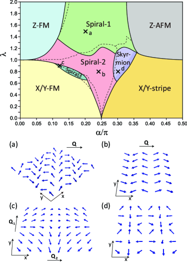
Figure 1: (Color online). Upper panel: Phase diagram for Eq. 1, calculated from TNS method. Z-FM (Z-AFM) denote the ferromagnetic (antiferromagnetic) phase with spin polarized along the $z$ direction, and X/Y means that the spins are polarized along either $x$ or $y$ direction. For a comparison the phase boundaries determined by classical simulations are shown in dashed lines. Lower panel: Spin textures of (a) Spiral-1 phase with spins spiral along ${\bf Q}={\bf e}_{x}-{\bf e}_{y}$ direction; (b) Spiral-2 phase with spins spiral along ${\bf Q}={\bf e}_{x}$ direction; (c) Spiral-3 phase spins spiral along both ${\bf Q}_{1}={\bf e}_{y}$ and ${\bf Q}_{2}={\bf e}_{x}$ directions; (d) 3$\times$3 skyrmion phase.

The following order parameters are used to distinguish different phases. Firstly, the static magnetic structure factor is defined as [$\mu=x,y,z$, $i=(i_{x},i_{y})$],

$$S^{\mu}(\textbf{k})=\frac{4}{L^{2}}\sum_{i,j}\langle S^{\mu}_{i}\cdot S^{\mu}_{j}\rangle e^{i[(i_{x}-j_{x})k_{x}+(i_{y}-j_{y})k_{y}]/L}.$$ (2)

on a $L\times L$ square lattice. For the FM and AFM phases along $\mu$-direction, $S^{\mu}(\textbf{k})$ has peaks at ${\bf k}=(0,0)$ and $(\pi,\pi)$, respectively; and in the strip phase the strongest peaks happen at ${\bf k}=(0,\pi)$ or $(\pi,0)$. We also define the spiral and skyrmion order parameters in real space asZhang et al. (2015),

$$\text{Sp}_{\mu}(i,j)=16\langle{\theta}_{\mu}^{i}{\theta}_{\mu}^{j}\rangle,\quad\text{Sk}(i,j)=64\langle v_{s}^{i}v_{s}^{j}\rangle,$$ (3)

where $\theta_{x}^{i}=({\bf S}_{i}\times{\bf S}_{i+{\bf e}_{x}})_{y}$ and $\theta_{y}^{i}=({\bf S}_{i}\times{\bf S}_{i+{\bf e}_{y}})_{x}$ are related to the relative planer spin angles for spins at site $i$ and $i+{\bf e}_{\mu}$. To account for the three dimensional spin alignment effect, we define the spin volume constructed by the spins at the three neighboring sites as $v_{s}^{i}={\bf S}_{i}\cdot({\bf S}_{i+{\bf e}_{x}}\times{\bf S}_{i+{\bf e}_{y}})$. In the co-planar spiral phase, $v_{s}^{i}=0$ exactly, but it is nonzero in the skyrmion phases. To determine the long-range order of the system, we calculate the order parameters as

$$\text{Sp}_{\mu}=\sum_{i}{1\over L^{2}}|\text{Sp}_{\mu}(i,i+l)|,\text{Sk}=\sum_{i}{1\over L^{2}}|\text{Sk}(i,i+l)|,$$ (4)

where $l=(L/2,L/2)$ to make $|i-j|$ as large as possible and $i$ is averaged over the whole lattice for better numerical accuracy.

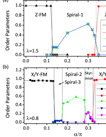
Figure 2: (Color online). Order parameters for the effective spin model derived from Bose-Hubbard model at (a) $\lambda=1.5$; and (b)$\lambda=0.8$, where $\text{Sp}_{\rm lg}$ [$\text{Sp}_{\rm sm}$] is the larger (smaller) one of $\text{Sp}_{x}$ and $\text{Sp}_{y}$ (see text for details).

Phase Diagram for Boson. The phase diagram is presented in Fig. 1 and corresponding order parameters are given in Fig. 2 at $\lambda$=1.5 and $\lambda$=0.8 and $\alpha\in[0,\pi/2]$. The spin model in Eq. 1 possesses some unique symmetries, which is crucial to understand this phase diagram. Firstly, the Hamiltonian in Eq. 1 is invariant upon operation $\alpha$$\rightarrow$$\pi-\alpha$ and $S_{i}^{x,y}\rightarrow-S_{i}^{x,y}$, which is equivalent to the transformation $U^{\dagger}_{\uparrow}b_{i\uparrow}U_{\uparrow}=-b_{i\uparrow}$, where $U_{\uparrow}=\exp(i\pi\sum_{i}n_{i\uparrow})$ in the original BH model. This symmetry directly leads to $U^{\dagger}_{\uparrow}H(\alpha,\lambda)U_{\uparrow}=H(\pi-\alpha,\lambda)$, i.e., the phase diagram should be symmetric about $\alpha={\pi\over 2}$. Therefore we only show the result for $\alpha\in[0,\pi/2]$.

We first discuss the phase diagram at four corners, where $\alpha\sim$ 0 or $\pi/2$ and $\lambda\ll 1$ or $\lambda\gg 1$. When $\alpha=0$, i.e., in the absence of SOC, the original spin model can be reduced to an effective XXZ spin model, with $J_{x}=J_{y}=-{1/\lambda}$, and $J_{z}=-{(2\lambda-1)/\lambda}$. When $\lambda>1$, $|J_{z}|>|J_{x}|$, the ground state is a Z-FM state, i.e., all spins are ferromagneticlly aligned along the $z$ direction. Our TNS calculations show that for small $\alpha\lesssim$0.15, the ground state is still Z-FM, as determined by the order parameters shown in Fig. 2a. In this region, the quantum simulations yield the same ground state as the classic one, suggesting the minor role of quantum fluctuation effect.

Interestingly, at $\alpha={\pi\over 2}$, the model can be mapped to the $\alpha$=0 case via a symmetry transformation, $\mathcal{U}=\prod_{i}e^{-i{\pi\over 2}i_{x}\sigma_{x}}e^{-i{\pi\over 2}i_{y}\sigma_{y}}$, i.e., $\mathcal{U}^{\dagger}H_{\pi\over 2}\mathcal{U}=H_{0}$. Use this transformation, we immediately see that the ground state near $\alpha={\pi\over 2}$ is a Z-AFM. We therefore see that these two limits ($\alpha$=0 and $\alpha$=${\pi\over 2}$) should have the exact same energies, and the quantum effects are small in both phases, which are confirmed by the numerical results.

However, there are dramatic difference in the case of $\lambda<$1 where the in-plane exchange energy dominates. The order parameters calculated by TNS at $\lambda$=0.8 are shown in Fig. 2. In the region of 0 $<\alpha/\pi<$ 0.13, the ground state is a FM phase, with all spins are polarized along either $x$ or $y$ direction, which we denote as X/Y-FM phase. Remarkably this phase is very different from what is obtained from the classical spin model, which gives a rotational invariant FM state Cole et al. (2012) with all spins lay in the $x$-$y$ plane (dubbed as XY-FM). To understand this difference, we note that the in-plane rotational symmetry is not inherent of the original Hamiltonian, which possesses only $C_{4}$ symmetry. The rotational invariance of the ground state in the classic model is due to the accidental degeneracy because the ground state of classic model happen to has $S_{z}$=0. When quantum fluctuation is introduced, it breaks the accidental degeneracy and restore the $C_{4}$ symmetry of the original Hamiltonian, which therefore single out a ground state with lower energy than the classical solution. This is the known as order-by-disorder mechanismVillain et al. (1980); Shender (1982). Again, we can apply symmetry transformation $\mathcal{U}=\prod_{i}e^{-i{\pi\over 2}i_{x}\sigma_{x}}e^{-i{\pi\over 2}i_{y}\sigma_{y}}$ near $\alpha=\pi/2$, which yields a X/Y-stripe phase (as confirmed by numerical results) for quantum spin model, in contrast to the 2$\times$2 vortex state obtained from classical simulations.

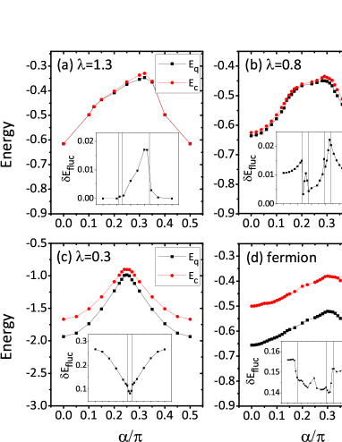
Figure 3: (Color online). Ground state energies from the classical ($E_{\text{c}}$) and quantum ($E_{\text{q}}$) simulations at (a) $\lambda=1.3$, (b) $\lambda=0.8$ and (c) $\lambda=0.3$ for boson, and (d) for fermion models. Insets give the corresponding fluctuation energy $\delta E_{\rm fluc}$. The vertical lines are the phase boundaries calculated by TNS.

The line $\lambda=0$ in principle can not he achieved due to the energy-costless double occupation. However this limit can still be defined in the sense of $\lim_{\lambda\rightarrow 0}\lambda H_{\lambda}=-\sum_{\langle i,j\rangle_{x}}[\cos(2\alpha)(S_{i}^{x}S_{j}^{x}+S_{i}^{z}S_{j}^{z})+S_{i}^{y}S_{j}^{y}]-\sum_{\langle i,j\rangle_{y}}[\cos(2\alpha)(S_{i}^{y}S_{j}^{y}+S_{i}^{z}S_{j}^{z})+S_{i}^{x}S_{j}^{x}]$. Obviously when $\alpha={\pi\over 4}$,

$$\lim_{\lambda\rightarrow 0}\lambda H_{\lambda,\alpha={\pi\over 4}}=-(\sum_{\langle i,j\rangle_{x}}S_{i}^{y}S_{j}^{y}+\sum_{\langle i,j\rangle_{y}}S_{i}^{x}S_{j}^{x})$$ (5)

which gives a compass model due to the strong coupling between the spins and directionsNussinov and Van Den Brink (2015). This model can not be solved exactly; however it can be shown exactly that the ground state is $2^{L+1}$-fold degenerated for a $L\times L$ square latticeDorier et al. (2005); You et al. (2010); Brzezicki and Oleś (2013). It therefore corresponds to a critical boundary between the X/Y-FM and X/Y stripe phases since any deviation from this critical point by varying the parameters ($\lambda$ and $\alpha$) can break the degeneracy and open an energy gap. The classical and quantum simulations yield the same critical point.

We next try to understand the spiral and skyrmion phases in the presence of strong DM interaction. The order parameters are shown in Eq. 4 (and the corresponding spin textures are shown in the lower panel of Fig. 1). The spiral-1 phase has two degenerate states spiral along either ${\bf e}_{x}+{\bf e}_{y}$ or ${\bf e}_{x}-{\bf e}_{y}$ direction. For these two cases the strongest peaks in the structure factor $S({\bf k})$ appear at ${\bf k}=\pm(k_{0},k_{0})$ and ${\bf k}=\pm(k_{0},-k_{0})$, respectively, where $k_{0}$ can be smoothly tuned by $\alpha$ and $\lambda$. However, due to the finite size used in the simulation, only $k_{0}$=$\frac{2\pi}{3}$, $\frac{\pi}{2}$, $\frac{\pi}{3}$ and $\frac{\pi}{6}$ are observed, which are commensurate with the system size. In this phase, the skyrmion order $\text{Sk}\sim 0$, whereas $\text{Sp}_{x}=\text{Sp}_{y}\neq 0$ are strongest among all the order parameters. The spiral-2 phase has two degenerate states, one is a spin spiral along $x$ direction, and other one is along $y$ direction. Therefore, only one of the order parameters, either $\text{Sp}_{x}$ or $\text{Sp}_{y}$ (see Fig. 2b) is nonzero. In contrast, in spiral-3 phase, $\text{Sp}_{x}$=$\text{Sp}_{y}$, both are nonzero. Spiral-3 phase is also observed in the classical model, and compared to the classical model, the spiral-3 phase region is greatly suppressed in the quantum model. In the skyrmion phase, the structure factor exhibits strongest peaks at ${\bf k}$=$(\pm k_{0},0)$ and $(0,\pm k_{0})$. Furthermore the non-conplaner of spin alinement induce a finite srkymion order Sk. The skyrmion phase is Neel typeKézsmárki et al. (2015) and has a period $3\times 3$ (light purple region in Fig. 1) or larger(dark purple region in Fig. 1), which is consistent with the numerical results for the classic spin model Cole et al. (2012).

To understand the quantum effects in a more quantitative way, we plot the ground state energies per site for $\lambda$=1.3, 0.8, 0.3 in Fig. 3 a - c respectively obtained from classical simulations ($E_{\rm c}$) and full quantum mechanical TNS simulations ($E_{\rm q}$). In the inserts, we also show the energy differences

$$\delta E_{\text{fluc}}=E_{\text{c}}-E_{\text{q}}\,.$$ (6)

Obviously $E_{\text{c}}\geq E_{\text{q}}$, thus $\delta E_{\text{fluc}}\geq 0$. From Fig. 3a. we find that when $\alpha=0$, and $\lambda$=1.3, $E_{\text{c}}=-0.61537$, and $E_{\text{q}}=-0.61538$ in the 12$\times$12 lattice, while the exact classical energy in a infinite size system is $E_{\text{c}}^{\infty}={2\lambda-1\over 2\lambda}=-0.61538$. This agreement can be understood using the Holstein-Primarkoff (HP) transformation to the XXZ model (see sup ) due to the disappearance of pairing (or condensate) term, thus $\delta E_{\text{fluc}}=0$ exactly. In fact the XXZ model can be used as a benchmark for the TNS method, which shows great accuracy in this problem. As shown in Fig. 3a, $\delta E_{\text{fluc}}\sim 0$ in the whole Z-FM and Z-AFM phase regimes, even when $\alpha\neq$0. In the spiral phase, $\delta E_{\text{fluc}}\sim$ 0.01 - 0.02 is more significant.

The fluctuation energy increases with the decreasing of $\lambda$. At $\lambda$=0.8, $\delta E_{\text{fluc}}\sim$0.01 in the X/Y-FM and X/Y strip phases, which is about 4% of the total energies. However, even though this energy difference seems not very large, the ground states predicted by classical model and quantum model are totally different. Full quantum treatments are therefore required to capture the correct physics in these phases. $\delta E_{\text{fluc}}$ is also different for different phases, which is most significant in the skyrmion phase, where $\delta E_{\text{fluc}}\sim$0.02. When $\lambda$ further decrease to 0.3, $\delta E_{\text{fluc}}$ increases dramatically. It is about 0.1 - 0.3 in the X/Y-FM and X/Y strip phases, which counts almost 10% - 20% of the total energies. The strong quantum fluctuation at small $\lambda$ suppresses the spiral-3 and skyrmion phases compared to the the classical phase diagram (see Fig. 1).

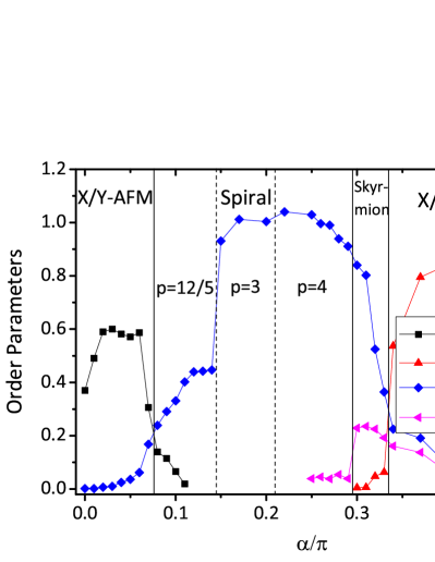
Figure 4: (Color online). Order parameters for the effective spin model derived from Fermi-Hubbard model.

Phase Diagrams for Fermion. For the spin model from FH model, we have $J=4t^{2}/U>$0, and $\lambda$=1. Therefore $\alpha$ serves as the only adjustable parameter in this model. The calculated phase diagram and the order parameters from the TNS method are presented in Fig. 4. Similar to the phase diagrams in the bosonic system, we find X/Y-AFM phase when $\alpha/\pi<0.08$ and X/Y-Stripe phase when $\alpha/\pi\in[0.34,0.5]$ (the mirror symmetry about $\alpha={\pi\over 2}$ is assumed). As before the classical model predicts a rotational invariant AFM and vortex phases in the $x$-$y$ plane, which reduce to the X/Y-AFM and X/Y-stripe phase due to order-by-order effect. Between the AFM and stripe phases, there are spiral phases and one skyrmion phase. The spiral phase may also be distinguished by the period $p={12\over 5},3,4$ which can be accommodated by our simulation sizes. In these phases the skyrmion order almost equal to zero and the spiral order dominates. However, when $\alpha/\pi\in[0.29,0.34]$ , the skyrmion order become important although the spiral order is still nonzero, similar to that in Fig. 2b.

The quantum fluctuation energy is much more pronounced in the FH model than in the BH model for all phases, as depicted in Fig.3d. For $\alpha$= 0, we find $E_{\text{c}}=-0.5$, and $E_{\text{q}}=-0.6579$, thus $\delta E_{\text{fluc}}=0.1579$. In the AFM and strip phases, $\delta E_{\text{fluc}}$ is about 30% of the total energy. The large quantum fluctuation energy in the AFM state is due to that there are vast Hilbert spaces near the $S$=0 that are energetically close to the ground state. The $\delta E_{\text{fluc}}$ is slightly small in the spiral phase and skyrmion phase, but still significant.

It is very interesting to note that the Z-AFM state in BH model however has very small $\delta E_{\text{fluc}}$, in sharp contrast with the AFM state derived from the FH model. To understand this difference, we note that the Z-AFM state in BH model can be mapped to the Z-FM state via symmetry transformations, which has small quantum fluctuation energy. Therefore, even though the two AFM states appear very similar to each other at the classical level, their physics are entirely different. More fundamentally, this difference is rooted from the different statistic properties between bosons and fermions.

Conclusion. We address the role of quantum fluctuation effect on the possibilities on observing the exotic spin structures in the spin-orbit coupled BH and FH models on a square lattice using TNS method. While for the out-of-plane FM and AFM phases the classical and quantum solution are the same, we find that the quantum order-by-disorder effect reduces the classical in-plane XY-FM and XY-vortex phases to the quantum X/Y-FM and X/Y-stripe phase. Moreover, the spiral phase and skyrmion phase can still be found even in the presence of quantum fluctuating effect. The structure of the phase diagrams are also understood from the symmetry point of view.

Acknowledgement. This work was funded by the Chinese National Science Foundation No. 11374275, 11474267, the National Key Research and Development Program of China No. 2016YFB0201202. M.G. acknowledges the support by the National Youth Thousand Talents Program No. KJ2030000001, the USTC start-up funding No. KY2030000053 and the CUHK RGC Grant No. 401113. The numerical calculations have been done on the USTC HPC facilities. M.G. Thank W. L. You for valuable discussion about compass model.

References

- McKay and DeMarco (2011) D. C. McKay and B. DeMarco, Reports on Progress in Physics 74, 054401 (2011).
- Bloch et al. (2008) I. Bloch, J. Dalibard, and W. Zwerger, Rev. Mod. Phys. 80, 885 (2008).
- Greiner et al. (2002) M. Greiner, O. Mandel, T. Esslinger, T. W. Hansch, and I. Bloch, Nature 415, 39 (2002).
- Jaksch et al. (1998) D. Jaksch, C. Bruder, J. I. Cirac, C. W. Gardiner, and P. Zoller, Phys. Rev. Lett. 81, 3108 (1998).
- Kuklov and Svistunov (2003) A. Kuklov and B. Svistunov, Physical review letters 90, 100401 (2003).
- Duan et al. (2003) L.-M. Duan, E. Demler, and M. D. Lukin, Phys. Rev. Lett. 91, 090402 (2003).
- Greif et al. (2013) D. Greif, T. Uehlinger, G. Jotzu, L. Tarruell, and T. Esslinger, Science 340, 1307 (2013).
- Kim et al. (2010) K. Kim, M.-S. Chang, S. Korenblit, R. Islam, E. Edwards, J. Freericks, G.-D. Lin, L.-M. Duan, and C. Monroe, Nature 465, 590 (2010).
- Simon et al. (2011) J. Simon, W. S. Bakr, R. Ma, M. E. Tai, P. M. Preiss, and M. Greiner, Nature 472, 307 (2011).
- Liu et al. (2009) X.-J. Liu, M. F. Borunda, X. Liu, and J. Sinova, Phys. Rev. Lett. 102, 046402 (2009).
- Lin et al. (2009) Y.-J. Lin, R. L. Compton, A. R. Perry, W. D. Phillips, J. V. Porto, and I. B. Spielman, Phys. Rev. Lett. 102, 130401 (2009).
- Wang et al. (2010) C. Wang, C. Gao, C.-M. Jian, and H. Zhai, Phys. Rev. Lett. 105, 160403 (2010).
- Lin et al. (2011) Y.-J. Lin, K. Jimenez-Garcia, and I. B. Spielman, Nature 471, 83 (2011).
- Ho and Zhang (2011) T.-L. Ho and S. Zhang, Phys. Rev. Lett. 107, 150403 (2011).
- Cong-Jun et al. (2011) W. Cong-Jun, I. Mondragon-Shem, and Z. Xiang-Fa, Chinese Physics Letters 28, 097102 (2011).
- Dalibard et al. (2011) J. Dalibard, F. Gerbier, G. Juzeliūnas, and P. Öhberg, Rev. Mod. Phys. 83, 1523 (2011).
- Campbell et al. (2011) D. L. Campbell, G. Juzeliūnas, and I. B. Spielman, Phys. Rev. A 84, 025602 (2011).
- Cheuk et al. (2012) L. W. Cheuk, A. T. Sommer, Z. Hadzibabic, T. Yefsah, W. S. Bakr, and M. W. Zwierlein, Phys. Rev. Lett. 109, 095302 (2012).
- Wang et al. (2012) P. Wang, Z.-Q. Yu, Z. Fu, J. Miao, L. Huang, S. Chai, H. Zhai, and J. Zhang, Phys. Rev. Lett. 109, 095301 (2012).
- Li et al. (2012) Y. Li, L. P. Pitaevskii, and S. Stringari, Phys. Rev. Lett. 108, 225301 (2012).
- Galitski and Spielman (2013) V. Galitski and I. B. Spielman, Nature 494, 49 (2013).
- Qu et al. (2013) C. Qu, C. Hamner, M. Gong, C. Zhang, and P. Engels, Phys. Rev. A 88, 021604 (2013).
- Hamner et al. (2014) C. Hamner, C. Qu, Y. Zhang, J. Chang, M. Gong, C. Zhang, and P. Engels, Nat Commun 5, 4023 (2014).
- Jiménez-García et al. (2015) K. Jiménez-García, L. J. LeBlanc, R. A. Williams, M. C. Beeler, C. Qu, M. Gong, C. Zhang, and I. B. Spielman, Phys. Rev. Lett. 114, 125301 (2015).
- Li et al. (2016) J. Li, W. Huang, B. Shteynas, S. Burchesky, F. Top, E. Su, J. Lee, A. O. Jamison, and W. Ketterle, Phys. Rev. Lett. 117, 185301 (2016).
- Wu et al. (2016) Z. Wu, L. Zhang, W. Sun, X.-T. Xu, B.-Z. Wang, S.-C. Ji, Y. Deng, S. Chen, X.-J. Liu, and J.-W. Pan, Science 354, 83 (2016).
- Huang et al. (2016) L. Huang, Z. Meng, P. Wang, P. Peng, S.-L. Zhang, L. Chen, D. Li, Q. Zhou, and J. Zhang, Nat. Phys. 12, 540 (2016).
- Dzyaloshinsky (1958) I. Dzyaloshinsky, J. Phys. Chem. Solids 4, 241 (1958).
- Moriya (1960) T. Moriya, Phys. Rev. 120, 91 (1960).
- Sergienko and Dagotto (2006) I. A. Sergienko and E. Dagotto, Phys. Rev. B 73, 094434 (2006).
- Cao et al. (2009) K. Cao, G.-C. Guo, D. Vanderbilt, and L. He, Phys. Rev. Lett. 103, 257201 (2009).
- Mühlbauer et al. (2009) S. Mühlbauer, B. Binz, F. Jonietz, C. Pfleiderer, A. Rosch, A. Neubauer, R. Georgii, and P. Böni, Science 323, 915 (2009).
- Mochizuki et al. (2010) M. Mochizuki, N. Furukawa, and N. Nagaosa, Phys. Rev. Lett. 104, 177206 (2010).
- Tokura and Seki (2010) Y. Tokura and S. Seki, Advanced Materials 22, 1554 (2010).
- Yu et al. (2010) X. Z. Yu, Y. Onose, N. Kanazawa, J. H. Park, J. H. Han, Y. Matsui, N. Nagaosa, and Y. Tokura, Nature. 465, 901 (2010).
- Heinze et al. (2011) S. Heinze, K. von Bergmann, M. Menzel, J. Brede, A. Kubetzka, R. Wiesendanger, G. Bihlmayer, and S. Blugel, Nat. Phys. 7, 713 (2011).
- Seki et al. (2012) S. Seki, X. Z. Yu, S. Ishiwata, and Y. Tokura, Science 336, 198 (2012).
- Nagaosa and Tokura (2013) N. Nagaosa and Y. Tokura, Nat. Nano. 8, 899 (2013).
- Wilson et al. (2014) M. N. Wilson, A. B. Butenko, A. N. Bogdanov, and T. L. Monchesky, Phys. Rev. B 89, 094411 (2014).
- Radić et al. (2012) J. Radić, A. Di Ciolo, K. Sun, and V. Galitski, Phys. Rev. Lett. 109, 085303 (2012).
- Cole et al. (2012) W. S. Cole, S. Zhang, A. Paramekanti, and N. Trivedi, Phys. Rev. Lett. 109, 085302 (2012).
- Gong et al. (2015) M. Gong, Y. Qian, M. Yan, V. W. Scarola, and C. Zhang, Sci. Rep. 5, 10050 (2015).
- Roszler et al. (2006) U. Roszler, A. N. Bogdanov, and C. Pfleiderer, Nature 442, 797 (2006).
- Rowland et al. (2016) J. Rowland, S. Banerjee, and M. Randeria, Phys. Rev. B 93, 020404 (2016).
- He et al. (2015) L. He, A. Ji, and W. Hofstetter, Physical Review A 92, 023630 (2015).
- Sun et al. (2015) F. Sun, J. Ye, and W.-M. Liu, Phys. Rev. A 92, 043609 (2015).
- Sun et al. (a) F. Sun, J. Ye, and W.-M. Liu, (a), arXiv:cond-mat/1603.00451 .
- Sun et al. (b) F. Sun, J. Ye, and W.-M. Liu, (b), arXiv:cond-mat/1601.01642 .
- Vidal (2003) G. Vidal, Phys. Rev. Lett. 91, 147902 (2003).
- Verstraete and Cirac (2004) F. Verstraete and J. I. Cirac, cond-mat/0407066 (2004).
- Sandvik and Vidal (2007) A. W. Sandvik and G. Vidal, Phys. Rev. Lett. 99, 220602 (2007).
- Schuch et al. (2008) N. Schuch, M. M. Wolf, F. Verstraete, and J. I. Cirac, Phys. Rev. Lett. 100, 040501 (2008).
- Song and Clay (2014) J.-P. Song and R. T. Clay, Phys. Rev. B 89, 075101 (2014).
- (54) See Supplemental Material, which includes Refs.Schuch et al. (2008); Wang et al. (2013); Liu et al. (2015); Swendsen and Wang (1986); Geyer (1991); Holstein and Primakoff (1940), for details of the string bond states method and the Holstein-Primarkov transformation.
- Zhang et al. (2015) S. Zhang, W. S. Cole, A. Paramekanti, and N. Trivedi, Annual Review of Cold Atoms and Molecules 3, 135 (2015).
- Villain et al. (1980) J. Villain, R. Bidaux, J.-P. Carton, and R. Conte, Journal de Physique 41, 1263 (1980).
- Shender (1982) E. F. Shender, Sov. Phys. JETP 56, 178 (1982).
- Nussinov and Van Den Brink (2015) Z. Nussinov and J. Van Den Brink, Rev. Mod. Phys. 87, 1 (2015).
- Dorier et al. (2005) J. Dorier, F. Becca, and F. Mila, Phys. Rev. B 72, 024448 (2005).
- You et al. (2010) W.-L. You, G.-S. Tian, and H.-Q. Lin, Journal of Physics A: Mathematical and Theoretical 43, 275001 (2010).
- Brzezicki and Oleś (2013) W. Brzezicki and A. M. Oleś, Phys. Rev. B 87, 214421 (2013).
- Kézsmárki et al. (2015) I. Kézsmárki, S. Bordács, P. Milde, E. Neuber, L. Eng, J. White, H. M. Rønnow, C. Dewhurst, M. Mochizuki, K. Yanai, et al., Nature materials 14, 1116 (2015).
- Wang et al. (2013) Z. Wang, Y. Han, G.-C. Guo, and L. He, Phys. Rev. B 88, 121105 (2013).
- Liu et al. (2015) W. Liu, C. Wang, Y. Li, Y. Lao, Y. Han, G.-C. Guo, and L. He, J. Phys.: Condens. Matter. 27, 085601 (2015).
- Swendsen and Wang (1986) R. H. Swendsen and J.-S. Wang, Phys. Rev. Lett. 57, 2607 (1986).
- Geyer (1991) C. J. Geyer, Computer Science and Statistics, Proceedings of the 23rd Symposium on the interface (Interface Foundation, 1991).
- Holstein and Primakoff (1940) T. Holstein and H. Primakoff, Phys. Rev. 58, 1098 (1940).