Dependence of Weak Interaction Rates on the Nuclear Composition during Stellar Core Collapse

Abstract

We investigate the influences of the nuclear composition on the weak interaction rates of heavy nuclei during the core collapse of massive stars. The nuclear abundances in nuclear statistical equilibrium (NSE) are calculated by some equation of state (EOS) models including in-medium effects on nuclear masses. We systematically examine the sensitivities of electron capture and neutrino-nucleus scattering on heavy nuclei to the nuclear shell effects and the single nucleus approximation. We find that the washout of shell effects at high temperatures brings significant change to weak rates by smoothing the nuclear abundance distribution: the electron capture rate decreases by $\sim$20$\%$ in the early phase and increases by $\sim$40$\%$ in the late phase at most, while the cross section for neutrino-nucleus scattering is reduced by $\sim$ $15\%$. This is because the open-shell nuclei become abundant instead of those with closed neutron shells as the shell effects disappear. We also find that the single-nucleus description based on the average values leads to underestimations of weak rates. Electron captures and neutrino coherent scattering on heavy nuclei are reduced by $\sim$80$\%$ in the early phase and by $\sim$5$\%$ in the late phase, respectively. These results indicate that NSE like EOS accounting for shell washout is indispensable for the reliable estimation of weak interaction rates in simulations of core-collapse supernovae.

I Introduction

Reliable nuclear physics as input data is indispensable for simulations of core collapse supernovae which are considered to occur at the end of the evolution of massive stars and lead to the emissions of neutrinos and gravitational waves, the synthesis of heavy elements and the formations of a neutron star or a black hole Janka (2012); Kotake et al. (2012); Burrows (2013). One of the underlying problems in these events is the uncertainties in input data for numerical simulations such as the equation of state (EOS) and weak interaction rate for hot and dense matter. Supernova matter is composed of nucleons, nuclei, electrons, photons and neutrinos and its temperature is high enough to achieve chemical equilibrium for all strong and electromagnetic reactions. The composition of nuclear matter is determined as a function of temperature $T$, density $\rho_{B}$ and electron fraction $Y_{e}$ by EOS models. The weak interactions on the nuclear components play important roles in the dynamics of core collapse supernovae through the evolution of the lepton fraction (Hix et al., 2003; Lentz et al., 2012).

Nuclear composition depends on the models employed for nuclei and nuclear matter and is affected by uncertainties. These equally come from finite density and temperature effects (Aymard et al., 2014; Agrawal et al., 2014; Steiner et al., 2013; Buyukcizmeci et al., 2013) and neutron/proton composition not yet produced and studied in terrestrial laboratories. Roughly speaking, there are two types of EOS models for supernova simulations. The single nucleus approximation (SNA), widely used over the past 2 decades, considers that the ensemble of heavy nuclei may be represented by a single nucleus Lattimer and Swesty (1991); Shen et al. (1998a, b, 2011). As a consequence, it can not account for the whole nuclear composition, which is indispensable for an accurate estimation of weak interaction rates. Furthermore, even the average mass and proton numbers and mass fraction of heavy nuclei may not be reproduced correctly by the representative nucleus Burrows and Lattimer (1984); Furusawa and Mishustin (2016). The other type of EOS model is the multi-nucleus EOS, in which the full ensemble of nuclei is solved and nuclear statistical equilibrium (NSE) abundance is obtained for each set of thermodynamical conditions Botvina and Mishustin (2004, 2010); Buyukcizmeci et al. (2014); Hempel and Schaffner-Bielich (2010); Shen et al. (2011).

We constructed an multi-nucleus EOS including various in-medium effects such as formation of nuclear pastas and washout of shell effects of heavy nuclei Furusawa et al. (2011, 2013, 2017). The shell effects are derived from the structure of nuclei in the ground state and smeared out completely at $T\sim$ 2.0 - 3.0 MeV (Brack and Quentin, 1974; Bohr and Mottelson, 1998; Sandulescu et al., 1997; Nishimura and Takano, 2014). This washout effect changes the nuclear component considerably Furusawa et al. (2017), whereas it has not been taken into account in all supernova EOS models. In most EOS models Lattimer and Swesty (1991); Shen et al. (1998a, b, 2011); Botvina and Mishustin (2004, 2010); Buyukcizmeci et al. (2014), shell effects are neglected in the first place and set to be completely smeared out even at zero temperature. Other EOS models assume full shell effects at any temperature Hempel and Schaffner-Bielich (2010); Shen et al. (2011). Some works, however, show that the evaluation of shell energies makes a large difference in the nuclear composition Furusawa et al. (2011); Buyukcizmeci et al. (2013). Recently, Raduta et al. reported that the shell quenching, which is a drop in the shell effect for neutron rich nuclei, affects up to $\sim$30$\%$ of the average electron capture rate during the core collapse owing to the modification of NSE abundance Raduta et al. (2016).

Neutrino scattering and electron capture on heavy nuclei are the main weak interactions in collapsing cores to determine the evolution of lepton fraction and the size of bounce cores. Those reaction rates at given ($\rho_{B},T,Y_{e}$) are obtained by folding the NSE abundance with the individual rates of all nuclei. When the single-nucleus EOS is utilized to calculate them, we have no choice but to substitute the representative nucleus for the ensemble of heavy nuclei. Even with the multi-nucleus EOS, we often estimate the weak rates by using the average values, such as average mass and proton numbers of nuclear ensemble, which are generally listed in EOS data tables for simulations. These prescriptions in the single nucleus descriptions may bear artificial errors from the complete folding results.

The calculation of electron captures contains more ambiguities than that of neutrino-nucleus scattering and provides a large uncertainty in supernova simulations. To obtain the total electron capture rates, we need the rates of individual nuclei. The first tabulated data of these, based on shell model calculations, was provided by Fuller et al. (FFN Fuller et al. (1982)). Oda et al. (ODA Oda et al. (1994)) and Langanke $\&$ Mart$\rm{\acute{\i}}$nez-Pinedo (LMP Langanke and Martínez-Pinedo (2000)) constructed tabulated data for sd- and pf-shell nuclei, respectively, based on shell model calculations with effective interactions and experimental energy levels. Langanke et al. (LMSH Langanke et al. (2003)) employed the Monte Carlo approach with a random phase approximation (RPA) for heavier nuclei in the pfg/sdg-shell. Unfortunately, these calculations for electron capture rates were aimed at nuclei along the $\beta-$stable line, whereas collapsing cores encounter the neutron-rich nuclei such as  ⁷⁸Ni, whose rates are yet to be developed from sophisticated models Sullivan et al. (2016). In general, we adopt any approximation formula for the nuclei with no data available.

For decades, the approximation formula for electron-captures provided by Bruenn Bruenn (1985) has been widely utilized, it has been pointed out that the formula underestimates the rates at finite temperature, since they ignored the thermal excitation of neutrons in the daughter nucleus and cut off the reactions for the nuclei with the neutron numbers larger than $40$ Langanke et al. (2003). It is known that the adoption of the Bruenn’s rate for the representative nucleus of SNA results in the overestimations of the lepton fraction and mass of bounce core and, hence, we should utilize more sophisticated data or formula with the NSE like EOS Hix et al. (2003); Langanke et al. (2003); Lentz et al. (2012). Juodagalvis et al. Juodagalvis et al. (2010) calculated the electron capture rates of nuclei more than 2200 based on the same RPA technique for LMSH with a Fermi – Dirac parametrization and constructed the data averaged over NSE abundance, although the individual rates were not released. We used their data in supernova simulations Nagakura et al. (2016), but the nuclear composition may be inconsistent between the NSE calculation used in the preparation for their data and our EOS model that includes in-medium effects and was adopted in the simulations Furusawa et al. (2013).

The purpose of this study is to clarify the impact of the uncertainties in the nuclear composition provided by EOS models on weak interaction rates. We focus on the shell effects of heavy nuclei, especially on the washout of them. We also report the deviation of the approximate weak rates for the average values and the most probable nucleus in the single nucleus descriptions from the accurate rates obtained with NSE abundances and individual rates.

This article is organized as follows. The EOS models and the nuclear compositions realized in the collapsing core are described in section II. In section III, we discuss the weak interaction rates based on them with emphases on the impact of shell effects and the errors of SNA. The paper is wrapped up with a summary and some discussions in section IV.

II Equation of state and nuclear composition

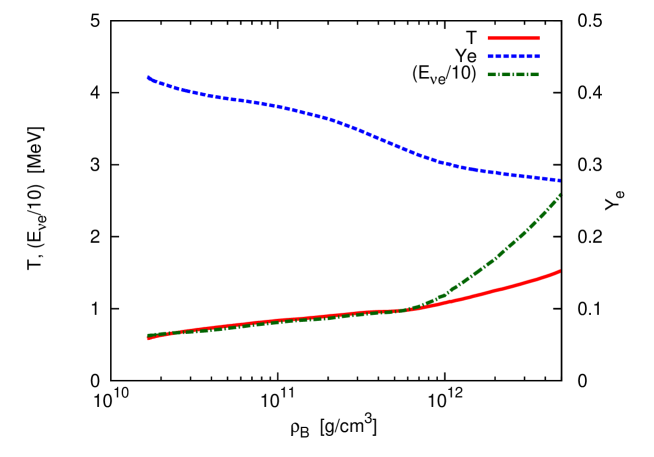
Figure 1: Temperature (red solid line), electron fraction (blue dashed line) and average energy of electron-type neutrinos (green dashed-dotted line) as a function of density at the center of the collapsing core in the reference supernova simulation of 11.2 ${\rm M_{\odot}}$ progenitor Nagakura et al. (2016).

We calculate the nuclear abundance in collapsing cores based on the EOS models, the details of which are given in Furusawa et al. Furusawa et al. (2011, 2013, 2017). The thermodynamical states are given by $T$, $\rho_{B}$ and $Y_{e}$ and those values in the center of the collapsing core are taken from a recent supernova simulation Nagakura et al. (2016) with the progenitor of 11.2 ${\rm M_{\odot}}$ Woosley et al. (2002). In the simulation, the Boltzmann neutrino-radiation hydrodynamics is exactly solved in spherical symmetry. We utilize the previous version of our EOS Furusawa et al. (2013) and the data of electron capture rates provided by Juodagalvis et al. Juodagalvis et al. (2010). Figure 1 shows the evolutions of $T$ and $Y_{e}$ as functions of $\rho_{B}$ at the center of the collapsing core before the core bounce. The simulation starts at $\rho_{B}\sim 2\times 10^{10}$  g/cm³ and the core bounce occurs when the central density reaches $\rho_{B}\sim 3\times 10^{14}$  g/cm³.

The model free energy density of our EOS reproduces the ordinary NSE results at low densities and temperatures and makes a continuous transition to the supra-nuclear density EOS. The thermodynamical quantities and nuclear abundances as functions of $\rho_{B}$, $T$ and $Y_{e}$ are obtained by minimizing the model free energy with respect to the number densities of nuclei and nucleons under the baryon and charge conservations. The model free energy is expressed as

$$\ f=f_{p,n}+\sum_{j}{n_{j}(E^{t}_{j}+M_{j})}+\sum_{i}{n_{i}(E^{t}_{i}+M_{i})},$$ (1)

where $n_{j/i}$ is the number density of the individual nucleus, index $j$ specifying a light nucleus with the proton number $Z_{j}\leq 5$ and index $i$ meaning a heavy nucleus with $6\leq Z_{i}\leq 1000$. The free energy density of the nucleon vapor outside nuclei $f_{p,n}$ is calculated by the relativistic mean field (RMF) with the TM1 parameter set Sugahara and Toki (1994). The translational energies of heavy and light nuclei $E^{t}_{i/j}$ are based on that for the ideal Boltzmann gas with the same excluded-volume effect as that in Lattimer’s EOS Lattimer and Swesty (1991). The masses of light nuclei, $M_{j}$, are evaluated by a quantum approach, in which the self- and Pauli-energy shifts are taken into account Typel et al. (2010); Röpke (2009). The masses of heavy nuclei are assumed to be the sum of bulk, Coulomb, surface and shell energies: $M_{i}=E_{i}^{B}+E_{i}^{C}+E_{i}^{Su}+E_{i}^{Sh}$. The bulk energies are obtained via the same RMF for free nucleons, while various modifications at finite density and temperature are accounted for in evaluations of surface and Coulomb energies.

The shell energies at zero temperature, $E_{i0}^{Sh}$, are obtained from the experimental or theoretical mass data Audi et al. (2012); Koura et al. (2005) by subtracting our liquid drop mass formula, which does not include the shell effects, $(M_{i}^{LDM}=E_{i}^{B}+E_{i}^{C}+E_{i}^{Su})$ in the vacuum limit as $E_{i0}^{Sh}=M_{i}^{data}-[M_{i}^{LDM}]_{vacuum}$. We take the washout of the shell effect into account approximately as follows:

$$E_{i}^{Sh}(T)=E_{i0}^{Sh}\displaystyle{\frac{\tau}{{\rm sinh}\tau}}.$$ (2)

The factor $\tau/{\rm sinh}\tau$ is derived by the analytical study for the single particle motion of nucleon outside the closed shell (Bohr and Mottelson, 1998). The normalized factor $\tau$ is defined as $\tau=2\pi^{2}T/\epsilon_{sh}$ with the energy spacing of the shells, $\epsilon_{sh}=41A_{i}^{-1/3}$ MeV, where $A_{i}$ is the mass number of nucleus $i$. This formulation can reproduce the feature of washout in that the shell energies disappear around $T\sim$ 2.0－3.0 MeV. Note that we ignore the density dependence of shell effects, which is considered in the original EOS models Furusawa et al. (2011, 2017), for simplicity and since it is negligible in this study.

To clarify the impact of the shell washout on weak rates, we prepare Models FS (full shells), WS (washout shells) and NS (no shells). Model FS ignores the washout, dropping the factor $\tau/{\rm sinh}\tau$ in Eq. (2). They may be regarded as a surrogate for the ordinary NSE calculations Timmes and Arnett (1999); Hempel and Schaffner-Bielich (2010), which also neglect the washout effect, but are widely utilized to estimate electron capture rates in supernova matter Juodagalvis et al. (2010); Sullivan et al. (2016). The previous version of our EOS used in the reference supernova simulation also lacks this effect Furusawa et al. (2013); Nagakura et al. (2016). Model WS is the new EOS Furusawa et al. (2017), in which we take it. We also prepare Model NS for comparison, in which the shell effects themselves are not considered at all ($E_{i0}^{Sh}=0$). This model is similar to the EOS models Lattimer and Swesty (1991); Shen et al. (2011); Buyukcizmeci et al. (2013), in which nuclear masses are evaluated without shell effects.

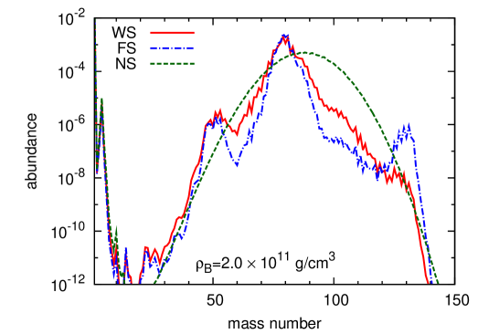
Figure 2: Abundances of elements as a function of the mass number for Models WS (red solid lines), FS (blue dashed-dotted lines) and NS (green dashed lines) at ($\rho_{B}$ [g/cm³], $T$ [MeV], $Y_{e}$)= (2.0 $\times 10^{10}$, 0.63, 0.41), (2.0 $\times 10^{11}$, 0.90, 0.36) and (2.0 $\times 10^{12}$, 1.25, 0.29) from top to bottom.

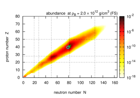
Figure 3: Nuclear abundances in the $(N,Z)$ plane at $\rho_{B}=2.0\times 10^{12}$ g/cm³, $T=1.25$ MeV, and $Y_{e}=0.29$ for Models FS (top), WS (middle) and NS (bottom) from top to bottom. The cyan circled dot and green cross indicate the average values and most probable nucleus, respectively. Dotted lines are neutron and proton magic numbers.

We calculate nuclear compositions by the fragment definitions for the thermodynamical states at the center of the collapsing core, which are given in Figure 1. Figure 2 shows the abundances of elements as a function of the mass number at ($\rho_{B}$ [g/cm³], $T$ [MeV], $Y_{e}$)= (2.0 $\times 10^{10}$, 0.63, 0.41), (2.0 $\times 10^{11}$, 0.90, 0.36) and (2.0 $\times 10^{12}$, 1.25, 0.29), which are defined as $\displaystyle{\sum_{Z_{i}+N_{i}=A}n_{i}/n_{B}}$, where $n_{B}$ is the baryon number density. We can see from the comparison of Models FS and WS that the washout effect has no influence on the nuclear composition at $\rho_{B}=2.0\times 10^{10}$ g/cm³, whereas the mass distributions in Model WS are smoother compared to those in Model FS at $\rho_{B}=2.0\times 10^{11}$ and 10¹² g/cm³. We can also find that this effect reduces the sharpness of the peaks at the neutron magic numbers $N=28,50$ and $82$ ($A\sim 50,80$ and 130) in the element distributions; especially the abundances around the third peak of $N=82$ is reduced more because of the smaller energy spacing, $\epsilon_{sh}$, for nuclei with the larger $A$ as discussed in Furusawa et al. Furusawa et al. (2017). Figure 3 displays nuclear abundances, $n_{i}/n_{B}$, in the $(N,Z)$ plane for the three models at $\rho_{B}=2.0\times 10^{12}$  g/cm³. It is clear that nuclei are abundant in the vicinities of the neutron magic numbers in Model FS. On the other hand, the nuclear distribution is much smoother in Model NS than that in Model FS. The effect of shell washout in Model WS provides an intermediate distribution between those of Models FS and NS.

Figure 4 shows the total mass fraction and average mass and proton numbers for heavy nuclei ($Z\geq 6$) as functions of the central density. They are defined as $X_{H}=\sum_{i}A_{i}n_{i}/n_{B}$, $\bar{A}=\sum_{i}A_{i}n_{i}/\sum_{i}n_{i}$ and $\bar{Z}=\sum_{i}Z_{i}n_{i}/\sum_{i}n_{i}$. The mass and proton numbers of the most probable nucleus in the ensemble of heavy nuclei, $A_{\rm mp}$ and $Z_{\rm mp}$, are also displayed. We find that the washout of shell effect reduces the mass fraction of heavy nuclei under the considered thermodynamical conditions, whereas the reduction is smaller than a few percent owing to the fact that the closed-shell nuclei decrease at the same time as the open-shell ones increase as shown in Figure 3. The re-distribution of heavy nuclei, especially reduction of the peak nuclei, alters chemical potentials of nucleons, thereby affecting, a little, the balance between heavy nuclei and the other baryons of nucleons and light nuclei. Note that the total mass fraction of heavy nuclei is not necessarily reduced by the shell suppression Furusawa et al. (2017). The average mass and proton numbers in Model WS do not always settle down to values between those in Models FS and NS, since shell effects are sensitive to the nuclear species and the washout affects the average values non-linearly. The mass and proton numbers of the most probable nucleus deviate from the average values in Models FS and WS due to shell effects, whereas they show close agreement in Model NS. Note that the neutrinos can barely escape from the core after the neutrino sphere is formed around $\rho_{B}\sim 2\times 10^{12}$  g/cm³. Therefore, the lepton fraction of the core is little reduced by weak interactions above this density Sullivan et al. (2016). We, hence, focus only on the densities lower than $\rho_{B}\sim 2\times 10^{12}$  g/cm³.

III Weak interaction rates

The electron capture rate of each nucleus is estimated by the weak rate tables of FFN Fuller et al. (1982), ODA Oda et al. (1994), LMP Langanke and Martínez-Pinedo (2000) and LMSH Langanke et al. (2003). For the nuclei where no data are available, we utilize the following approximation formula as a function of the $Q$ value Fuller et al. (1985); Langanke et al. (2003):

$$\lambda_{i}=\frac{({\rm ln}2)B}{K}\left(\frac{T}{m_{e}c^{2}}\right)^{5}\left[F_{4}(\eta_{i})-2\chi_{i}F_{3}(\eta_{i})+\chi_{i}^{2}F_{2}(\eta_{i})\right],$$ (3)

where $K=6146$ sec, $\chi_{i}=(Q_{i}-\Delta E)/T$, $\eta_{i}=(\mu_{e}+Q_{i}-\Delta E)/T$ with the electron chemical potential $\mu_{e}$ and $F_{k}$ is the relativistic Fermi integral of order $k$. The parameters of a typical matrix element ($B=4.6$) and a transition energy from an excited state in the parent nucleus to a daughter state ($\Delta E=2.5$ MeV) are fitted to shell-model calculations for the pf-shell nuclei of LMP data by Langanke et al. Langanke et al. (2003). The $Q$ value of each nucleus, $Q_{i}$, is calculated by the mass formulae for heavy nuclei, which is introduced in the previous subsection, as $Q_{i}=M_{i}(Z_{i},N_{i})-M_{i}(Z_{i}-1,N_{i}+1)$ with in-medium effects at finite density and temperature. We adopt reaction rates in the predetermined order as LMP $>$ LMSH $>$ODA $>$FFN $>$ approximation formula, which means that rates from sources with higher orders are utilized for nuclei whose rates from multiple sources exist. Figure 5 shows the sources in nuclear chart, which are applied to each nuclei. The light nuclei ($Z\leq 5$) are ignored in this work, since they are not abundant under the considered thermodynamical conditions.

The neutrino-nucleus scattering rate is calculated for electron-type neutrinos with the average energy, $E_{\nu_{e}}$, whose values are taken from the result of the reference simulation and shown in Figure 1. The cross section of an individual nucleus is evaluated as

$$\sigma_{i}(E_{\nu_{e}})=\frac{G_{W}^{2}}{8\pi(\hbar c)^{4}}E_{\nu_{e}}^{2}A_{i}^{2}\left\{1-\frac{2Z_{i}}{A_{i}}(1-{\rm sin}^{2}\theta_{W})\right\}^{2}\frac{2y_{i}+{\rm exp}(2y_{i})-1}{y_{i}^{2}},$$ (4)

where $y_{i}=1.92\times 10^{-5}A_{i}^{2/3}E_{\nu_{e}}^{2}$, $G_{W}$ and $\theta_{W}$ are the weak coupling constant and Weinberg angle, respectively, and the isoenergetic zero-momentum transfer and non-degenerated nucleus are assumed Bruenn (1985).

III.1 Dependence of Weak Interaction Rates on Shell Effect

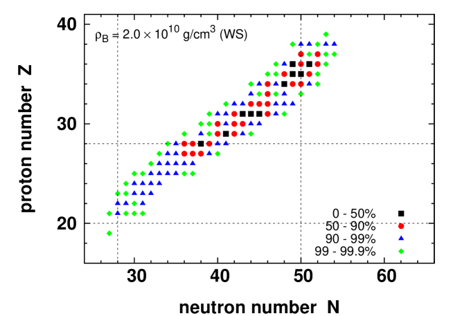
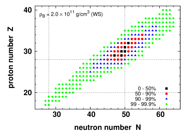
Figure 6: The nuclear species with the largest electron capture contribution, $n_{i}\lambda_{i}/n_{B}$, which account for the top 50$\%$ (black squares), 50-90$\%$ (red circles), 90-99$\%$ (blue triangles) and 99-99.9$\%$ (green diamonds) of the total electron capture rate per baryon $\lambda^{ec}$ for Model WS at $\rho_{B}=2.0\times 10^{10}$ g/cm³ (top panel) and $2.0\times 10^{11}$ g/cm³ (bottom panel). Dotted lines are neutron and proton magic numbers.

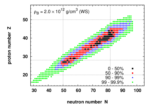
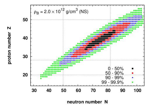
Figure 7: The nuclear species with the largest electron capture contribution, $n_{i}\lambda_{i}/n_{B}$, which account for the top 50$\%$ (black squares), 50-90$\%$ (red circles), 90-99$\%$ (blue triangles) and 99-99.9$\%$ (green diamonds) of the total electron capture rate per baryon $\lambda^{ec}$ for Models FS (top), WS (middle) and NS (bottom) at $\rho_{B}=2.0\times 10^{12}$ g/cm³. Dotted lines are neutron and proton magic numbers.

We discuss the contribution of each nucleus to the total electron capture rate per baryon defined as $\lambda^{ec}=\sum_{i}n_{i}\lambda_{i}/n_{B}$. Figure 6 shows the nuclei with the largest contributions, $n_{i}\lambda_{i}/n_{B}$, which make the top 50$\%$, 90$\%$, 99$\%$ and 99.9$\%$ of $\lambda^{ec}$ for Model WS at $\rho_{B}=2.0\times 10^{10}$ and $2.0\times 10^{11}$ g/cm³. At the beginning of collapse ($\rho_{B}=2.0\times 10^{10}$ g/cm³), the nuclei with $36\leq N\leq 52$ account for the top 90$\%$ of the total electron capture. On the other hand, the nuclei around the second peak ($45\leq N\leq 55$) make up $90\%$ at $\rho_{B}=2.0\times 10^{11}$ g/cm³. Figure 7 compares the nuclei with large contributions at $\rho_{B}=2.0\times 10^{12}$ g/cm³ for all models. The dominant nuclei correspond more or less to the nuclei with large abundances in Figure 3. For Model FS, two islands around $N=50$ and $82$ are clearly visible in the distribution due to shell effects. This feature has also been observed in the previous work Sullivan et al. (2016), in which the shell washout is neglected. On the other hand, the distributions of dominant nuclei for Models WS and NS are more broad and the non-magic nuclei such as ¹⁰⁵Kr ($N=69$) also contribute to the total rate. We also find that the numbers of the nuclei with large contributions increase as the shell effects become weaker; these are 10, 48 and 59 for the top 50$\%$ and 62, 175 and 188 for the top 90$\%$ in Models FS, WS and NS, respectively.

Figure 8 displays the electron capture rate of heavy nuclei per baryon $\lambda^{ec}$ as a function of central density, which corresponds to the time derivative of electron fraction in collapsing cores by the reactions, ${\rm d}Y_{e}/{\rm d}t$. Note that neutrino blocking is not considered here. The weak rate data (FFN, ODA, LMP and LMSH) are used whenever available in Models FS, WS and NS (Data+Appro.), whereas the approximation formula of Eq. (3) is applied to all nuclei in the model WS (Appro.). We can see from the comparison of models WS with and without the data, that the weak rate data are influential at densities below $\rho_{B}\sim 10^{11}$ g/cm³; this is because the nuclei that are not included in these data become abundant at high densities.

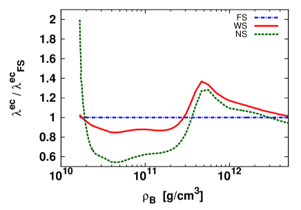
Figure 9: Ratio of electron capture rates per baryon $\lambda^{ec}$ (left panel) and those per nuclei, $\bar{\lambda}^{ec}=\sum_{i}n_{i}\lambda_{i}/(\sum_{i}n_{i})$, (right panel) for Models WS (red solid lines) and NS (green dashed lines) to those for Model FS (blue dashed-dotted lines) as a function of central density.

Figure 9 shows the ratio of electron capture rates for Models WS and NS to those for Model FS. The left panel compares the rates per baryon $\lambda^{ec}$, while the right panel displays those per nuclei $\bar{\lambda}^{ec}=\sum_{i}n_{i}\lambda_{i}/(\sum_{i}n_{i})$. They can be converted to each other as $\lambda^{ec}=\bar{\lambda}^{ec}X_{H}/\bar{A}$ by using $X_{H}$ and $\bar{A}$, which are shown in Figure 4. We find that the shell smearing cuts down on $\lambda^{ec}$ and $\bar{\lambda}^{ec}$ by $\sim 20\%$ at low densities and raises them by $\sim 40\%$ at high densities. At around $\rho_{B}=4\times 10^{10}$ g/cm³, Model FS displays the largest rates, since the mass fractions of the nuclei around the first peak with $N=28$ are the largest among the three models. These nuclei at the first peak of $A\sim 50$ ($N\sim 28$) have higher reaction rates than those of the nuclei with larger mass numbers. The reduction of nuclear abundance at the first peak results in lower electron capture rates in Model WS than those in Model FS. At densities greater than $\rho_{B}\sim 3\times 10^{11}$ g/cm³, Model WS yields higher rates than Model FS, since the magic nuclei are less and non-magic ones are more abundant as shown in Figures 2, 3 and 7. This feature is essentially similar to the result observed in Raduta et al. Raduta et al. (2016) in that shell quenching reduces the closed-shell nuclei and increases the averaged electron capture rate. Model WS has larger $\lambda^{ec}$ than Model NS because of larger nuclear abundances $\sum_{i}n_{i}$ (larger $X_{H}$ and smaller $\bar{A}$ as shown in Figure 4). On the other hand, the rates per nuclei, $\bar{\lambda}^{ec}$, in Model WS settle down to values between those in Models NS and FS. At densities greater than $\rho_{B}\sim 2\times 10^{12}$ g/cm³, all models lead to the same value of $\bar{\lambda}^{ec}$, since $\mu_{e}$ becomes much larger than the $Q$ values of nuclei and, as a result, their differences among nuclei become negligible.

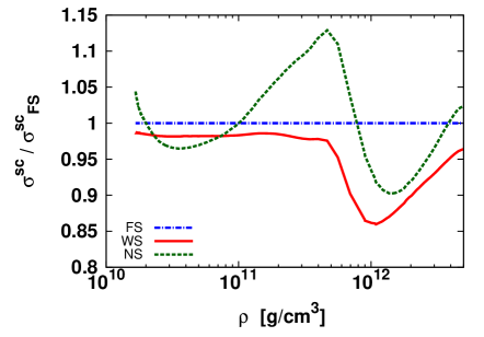
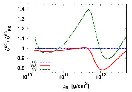
Figure 10: Ratio of cross sections of neutrino-nucleus scattering per baryon $\sigma^{sc}=\sum_{i}n_{i}\sigma_{i}/n_{B}$ (left panel) and those per nuclei $\bar{\sigma}^{sc}=\sum_{i}n_{i}\sigma_{i}/(\sum_{i}n_{i})$ (right panel) for Models WS (red solid lines) and NS (green dashed lines) to those for Model FS (blue dashed-dotted lines) as a function of central density.

Figure 10 displays the ratio of the cross sections of neutrino-nucleus scattering in Models WS and NS to those in Model FS. Left and right panels compare the cross sections per baryon $\sigma^{sc}=\sum_{i}n_{i}\sigma_{i}/n_{B}$ and those per nuclei $\bar{\sigma}^{sc}=\sum_{i}n_{i}\sigma_{i}/\sum_{i}n_{i}$, respectively. The proportional relation in Eq. (4), $\sigma_{i}\mathrel{\vbox{ \offinterlineskip\halign{\hfil$#$\cr\propto\cr\kern 2.0pt\cr\sim\cr\kern-2.0pt\cr}}}A_{i}^{2}$, gives the approximate relations of those rates as: $\sigma^{sc}\mathrel{\vbox{ \offinterlineskip\halign{\hfil$#$\cr\propto\cr\kern 2.0pt\cr\sim\cr\kern-2.0pt\cr}}}X_{H}\overline{A^{2}}/\overline{A}\sim X_{H}\overline{A}$ and $\bar{\sigma}^{sc}\mathrel{\vbox{ \offinterlineskip\halign{\hfil$#$\cr\propto\cr\kern 2.0pt\cr\sim\cr\kern-2.0pt\cr}}}\overline{A^{2}}\sim\overline{A}^{2}$, where $\overline{A^{2}}=\sum_{i}A_{i}^{2}n_{i}/\sum_{i}n_{i}$. The difference in $X_{H}$ is not very great as shown in Figure 4 and, hence, models with larger $\bar{A}$ lead to larger $\sigma^{sc}$ and $\bar{\sigma}^{sc}$. For instance, Model NS gives the greatest cross section at $\rho_{B}\sim 4\times 10^{11}$ g/cm³. We find that the washout of the shell effect reduces $\sigma^{sc}$ by $\sim 15\%$ around $\rho_{B}\sim 10^{12}$ g/cm³, since the nuclear abundances with large mass numbers decrease and $\overline{A}$ becomes small. The cross sections per nuclei, $\bar{\sigma}^{sc}$, are reduced more than $\sigma^{sc}$ and down about 20$\%$, since they are proportional to $A^{2}$.

III.2 Approximation Errors of Single Nucleus Description in Weak Rates

As explained in the Introduction, the single-nucleus EOS has been utilized in most supernova simulations, where the weak rates of the representative nucleus are substituted for the exact rates obtained by folding individual rates with NSE abundances. Even in the simulation with multi-nucleus EOS, the average values such as $\overline{A}$ and $\overline{Z}$ are utilized to estimate the neutrino-nucleus scattering just in the same way as in the single nucleus description. The same applies to the reference simulation of core collapse. In this subsection, we discuss the errors in the weak rates of the single nucleus descriptions.

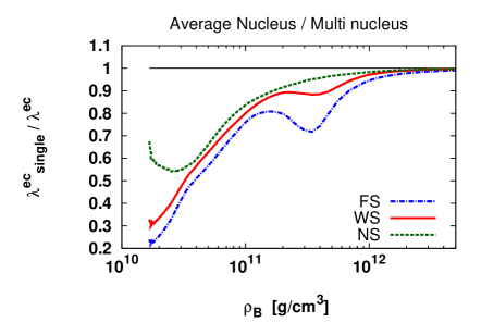
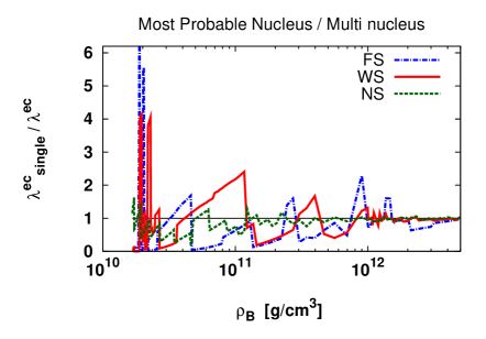
Figure 11: Electron capture rate per baryon of heavy nuclei as a function of central density for Model WS based on the multi-nucleus description with the parametrized rate provided by Langanke et al. Langanke et al. (2003) (red solid lines) and the Bruenn rate Bruenn (1985) (red dashed lines). Those of the average nucleus are shown for the former rate (cyan solid lines) and the latter (cyan dashed lines). The black dashed-dotted line shows that of the most probable nucleus for the former rate.

Figure 12: Ratio of electron capture rates in the single-nucleus descriptions to those of the multi-nucleus descriptions for Models WS (red solid lines), FS (blue solid lines) and NS (green solid lines). Left and right panels display those of the average nucleus and the most probable one.

We estimate the electron capture rates per baryon, $\lambda^{ec}_{\rm single}$, for the average nucleus and the most probable one in the single-nucleus descriptions, in which the representative nucleus is assumed to account for the total mass fraction of heavy nuclei $X_{H}$ alone. The former is expressed as $\lambda^{ec}_{\rm single}(\overline{Q},\overline{A})=X_{H}/\overline{A}\ \lambda(\overline{Q})$ with Eq. (3) on the assumption that the average nucleus has $\overline{A}$, $\overline{Z}$ and the average $Q$ value, $\overline{Q}$. The latter is defined as $\lambda^{ec}_{\rm single}(Q_{\rm mp},A_{\rm mp})=X_{H}/A_{\rm mp}\lambda(Q_{\rm mp})$ using the individual rate, $\lambda(Q_{\rm mp})$, and mass number, $A_{\rm mp}$, of the most probable nucleus. In the multi-nucleus description, Eq. (3) is applied to all nuclei as $\lambda^{ec}=\sum_{i}n_{i}\lambda(Q_{i})/n_{B}$. Note that weak rate tables are not used here for simplicity. Figure 12 shows these rates for Model WS and Figure 12 displays the ratio of $\lambda^{ec}_{\rm single}$ to $\lambda^{ec}$ for all models. It is clear to see that the electron capture rates based on the average values are smaller due to the neglect of the nuclei other than those at abundance peaks. The nuclei with smaller mass numbers and/or larger charge fractions $Z_{i}/A_{i}$, which are not included in the single nucleus description, have reaction rates higher than those of the nuclei at the abundance peak. This artificial error in Model FS is the largest among the three models, since the average values are the closest in value to those of the magic nuclei as shown in Figure 3, whose rates are lower than those of non-magic ones. We comment that the electron capture rates of the most probable nuclei are discrete, since $A_{\rm mp}$ and $Z_{\rm mp}$ adopt integer values and also $Q_{\rm mp}$ is not continuous either. They are underestimated more often than not, but basically do not follow the trend of average values especially in Models FS and WS because of shell effects.

Figure 12 also shows the electron capture rates based on the old formula provided by Bruenn Bruenn (1985). In this estimation, the reaction rate is set to be zero for the nuclei with $N\geq 40$ as already noted. We find that the formula is out of the question. The rate of average nucleus drops to zero just after the core-collapse starts, since the average neutron number exceeds 40. Even in the multi-nucleus description with the old formula, the rate decreases as the nuclei with $N<40$ diminish at high densities.

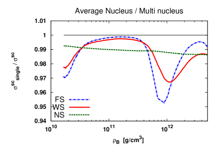
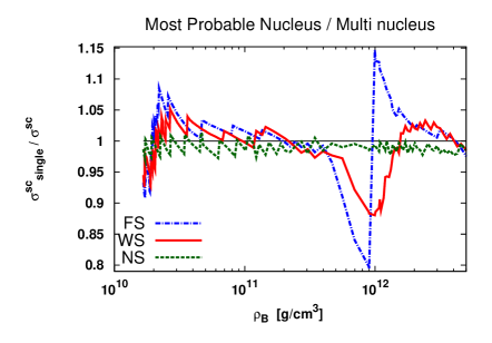
Figure 13: Ratio of cross sections of neutrino-nucleus scattering in the single-nucleus descriptions to those of the multi-nucleus descriptions for Models WS (red solid lines), FS (blue solid lines) and NS (green solid lines). Left and right panels display those of the average nucleus and the most probable one.

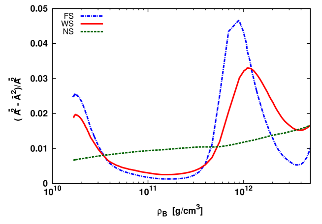
Figure 14: Dispersion of mass number normalized by the average mass number squared, $(\overline{A^{2}}-\overline{A}^{2})/\overline{A^{2}}$, as functions of central density for Models FS (blue dashed-dotted line), WS (red solid line) and NS (green dashed line).

Finally we compare the cross section per baryon for neutrino coherent scattering on heavy nuclei among the average nucleus ($\sigma^{sc}_{\rm single}(\bar{A},\bar{Z})=\sigma(\bar{A},\bar{Z})X_{H}/\bar{A}$), the most probable one ($\sigma^{sc}_{\rm single}(A_{\rm mp},Z_{\rm mp})=\sigma(A_{\rm mp},Z_{\rm mp})X_{H}/A_{\rm mp}$) and the multi-nucleus description ($\sigma^{sc}=\sum_{i}\{n_{i}\sigma(A_{i},Z_{i})\}/n_{B}$) in Figure 13. Unlike the electron capture, the scattering is not sensitive to the feature of the individual nucleus and its rate is roughly proportional to $A^{2}$. Hence, the approximation errors are not significantly large compared with electron captures. We find that the errors in the single nucleus description based on the average nucleus depend on the dispersion of mass numbers, $\overline{A^{2}}-\bar{A}^{2}$, as shown in Figure 14. In Models FS and WS, the dispersions are small, around $\rho_{B}\sim 10^{11}$ g/cm³, since closed-shell nuclei with $N=50$ dominate in the nuclear abundance. They grow steeply around $\rho_{B}\sim 10^{12}$ g/cm³, since the nuclei at the third peak $N=82$ appear and the average mass number rises as shown in Fig.4. In Model WS, the shell washout reduces the dispersion and, as a result, the approximation error is reduced. The errors are about 1$\%$, 3$\%$ and 5$\%$ at most for Models NS, WS and FS, respectively. The approximation errors for the most probable nuclei are larger than those for the average ones, although the deviations are smaller than those seen in the case of electron captures.

IV Summary and Discussion

We have calculated the weak interaction rates of heavy nuclei in the collapsing core of the massive star to investigate their sensitivities to uncertainties in nuclear composition. The abundance of various nuclei is evaluated by the three different EOS models. One is our new EOS model including the washout of shell effect, which has been ignored so far Furusawa et al. (2017). The other models are systematically formulated to drop the washout of shell effect or the shell effect itself. For the electron capture rates of individual nuclei, we have utilized the tabulated data of the individual nucleus, whenever available, and the approximation formula for the nuclei with no data available.

Utilizing the trajectory of density, temperature and electron fraction in the recent simulation of core-collapse, we have made a systematic comparison of the weak interaction rates derived with composition in the different EOS models. We show that not only nuclei with neutron magic numbers but also non-magic nuclei contribute to the total electron capture rates. We find that the washout of shell effect reduces the electron capture rates by $\sim 20\%$ at low densities and increases them by $\sim 40\%$ at high densities, while this effect also cuts down the neutrino-nucleus scattering by $\sim$ 15$\%$. These changes arise from the fact that the nuclei in the vicinity of the neutron magic numbers are reduced and other nuclei are populated instead. The improvement of the weak rates based on the EOS model accounting for shell washout would improve the supernova simulations.

We have investigated the gaps between single- and multi-nucleus EOS models by comparing the approximate weak rates for the average values and the most probable nucleus in single nucleus descriptions and the exact one for the full ensemble of nuclei. We find that the single-nucleus description based on the average nucleus underestimates electron capture rates by $\sim$ 80$\%$ at the beginning of core collapse due to the concentration of nuclear abundance in the vicinities of the neutron magic numbers. We have shown that the underestimation of neutrino-nucleus scattering is at most $\sim$5$\%$, the size of which depends on the dispersion of mass number. The weak rates for the most probable nuclei deviate more largely from the actual values than those for average ones.

In this study, we adopt the fitting formula of the electron capture rate of Eq. (3) for the heavy and/or neutron-rich nuclei, although it was parametrized for pf-shell nuclei which are close to the beta-stability line. The rates for such nuclei may diverge from what is predicted by the approximation formula Juodagalvis et al. (2008); Sullivan et al. (2016). In addition, the in-medium effects are not carefully considered in the calculation of weak rates. To obtain the precise weak rates during stellar core-collapse, we require the new experiments and theoretical studies which are aimed not only at magic nuclei but also at non-magic ones at finite densities and temperatures. Note that there remain various uncertainties in EOS models. Shell energies are simply assumed to be the difference between experimental or theoretical mass data and the original liquid drop model in our EOS. The free energy of nucleons and the bulk energy of heavy nuclei are calculated by the RMF with the TM1 parameter set in this study. The employment of another theory for them may also affect the nuclear component. We are also currently constructing an table for weak interaction based on the new EOS for supernova simulations, which will be available in the public domain. The supernova simulations with the improved weak rates and the impact of the update on the dynamics will be reported in the near future.

Figure 4: Mass fraction of heavy nuclei with $Z\geq 6$ as a function of central density for Models WS (red solid lines), FS (blue dashed-dotted lines) and NS (green dashed lines) in top panel. The bottom panel displays the average mass and proton numbers, $\overline{A}$ and $\overline{Z}$, (solid lines) and those of the most probable nuclei, $A_{\rm mp}$ and $Z_{\rm mp}$, (dashed lines) for Models WS (red), FS (blue) and NS (green).

Figure 5: The nuclear species, for which the data of FFN (blue squares), ODA (cyan squares), LMP (green squares), or LMSH (red squares), or approximation formula (yellow squares) for electron capture rate is adopted. Black circles represent stable nuclei and dashed black lines display the neutron and proton drip lines (dashed black lines), which are estimated by the KTUY mass formula Koura et al. (2005). A dashed-dotted line indicates the trajectory of average neutron and proton numbers of heavy nuclei in the center of collapsing cores, which is calculated by Model WS and shown in Figure 4 .

Figure 8: Electron capture rate per baryon of heavy nuclei, $\lambda^{ec}=\sum_{i}n_{i}\lambda_{i}/n_{B}$, as a function of central density for Models WS (red solid lines), FS (blue solid lines) and NS (green solid lines). The red dashed line shows the result for Model WS in which the approximation formula is adopted for all nuclei and weak rate data are not utilized.