A Geometric Description of Feasible Singular Values in the Tensor Train Format

Abstract

Tree tensor networks such as the tensor train format are a common tool for high dimensional problems. The associated multivariate rank and accordant tuples of singular values are based on different matricizations of the same tensor. While the behavior of such is as essential as in the matrix case, here the question about the feasibility of specific constellations arises: which prescribed tuples can be realized as singular values of a tensor and what is this feasible set?
We first show the equivalence of the tensor feasibility problem (TFP) to the quantum marginal problem (QMP). In higher dimensions, in case of the tensor train (TT-)format, the conditions for feasibility can be decoupled. By present results for three dimensions for the QMP, it then follows that the tuples of squared, feasible TT-singular values form polyhedral cones. We further establish a connection to eigenvalue relations of sums of Hermitian matrices, which in turn are described by sets of interlinked, so called honeycombs, as they have been introduced by Knutson and Tao.
Besides a large class of universal, necessary inequalities as well as the vertex description for a special, simpler instance, we present a linear programming algorithm to check feasibility and a simple, heuristic algorithm to construct representations of tensors with prescribed, feasible TT-singular values in parallel.

Keywords. tensor, TT-format, singular value, honeycomb, eigenvalue, Hermitian matrix, linear inequality, quantum marginal problem

AMS subject classifications. 15A18, 15A69, 52B12, 81P45

Introduction

For $\mathbb{K}\in\{\mathbb{R},\mathbb{C}\}$, let $A\in\mathbb{K}^{n_{1}\times\ldots\times n_{d}}$ be a $d$th-order tensor, such as in Fig. 1.

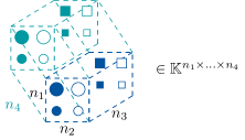
Figure 1: Visualization of a $4-$dimensional tensor $A$ with mode sizes $n_{1}=\ldots=n_{4}=2$.

The tensor $A$ allows to be reshaped into certain matricizations

$$A^{(\{1,\ldots,\mu\})}\in\mathbb{K}^{n_{1}\cdot\ldots\cdot n_{\mu}\ \times\ n_{\mu+1}\cdot\ldots\cdot n_{d}},\quad\mu=1,\ldots,d-1,$$

which are related to the so called tensor train (TT-)decomposition [12, 28]. The vectorization $\mathrm{vec}(\cdot)$ in co-lexicographic order (column-wise) is to be an invariant to these reshapings, i.e.

$$\mathrm{vec}(A^{(\{1,\ldots,\mu\})})=\mathrm{vec}(A)\in\mathbb{K}^{n_{1}\cdot\ldots\cdot n_{d}\times 1},\quad\mu=1,\ldots,d-1,$$

such that they become uniquely defined.
We may also explicitly write $A^{(\{1,\ldots,\mu\})}((i_{1},\ldots,i_{\mu})_{1},\,(i_{\mu+1},\ldots,i_{d})_{\mu+1})=A(i)$ where $(i_{1},\ldots,i_{\mu})_{\nu}:=1+\sum_{s=1}^{\mu}\left(\prod_{h=1}^{s-1}n_{\nu+h-1}\right)(i_{s}-1)\in\{1,\ldots,n_{\nu}\ldots n_{\nu+\mu-1}\}\subset\mathbb{N}$ (we will skip the index $\nu$ when context renders it obsolete).
The $d-1$ tuples of TT-singular values $\sigma=(\sigma^{(1)},\ldots,\sigma^{(d-1)})=\operatorname{sv}_{\mathrm{TT}}(A)$ and the according TT-rank(s) $r=(r_{1},\ldots,r_{d-1})\in\mathbb{N}^{d-1}$ of $A\neq 0$ are given through the matrix singular values $(\operatorname{sv})$ of its reshapings

$$\sigma^{(\mu)}:=\operatorname{sv}(A^{(\{1,\ldots,\mu\})}),\ r_{\mu}:=\operatorname{rank}(A^{(\{1,\ldots,\mu\})}),\quad\mu=1,\ldots,d-1,$$

such as displayed in Fig. 2.

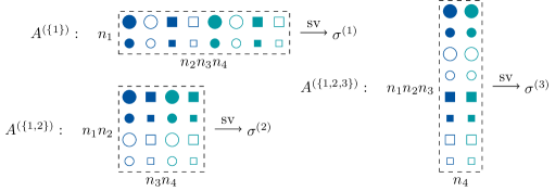
Figure 2: Matricizations (or reshapings, or unfoldings) of the $4$th-order tensor $A$ into the matrices $A^{(\{1\})}\in\mathbb{K}^{n_{1}\times n_{2}n_{3}n_{4}}$, $A^{(\{1,2\})}\in\mathbb{K}^{n_{1}n_{2}\times n_{3}n_{4}}$ and $A^{(\{1,2,3\})}\in\mathbb{K}^{n_{1}n_{2}n_{3}\times n_{4}}$ through which $\sigma=\operatorname{sv}_{\mathrm{TT}}(A)$ is obtained.

For simplicity, each of these singular values is considered to be a weakly decreasing, infinite sequence with finitely many nonzero entries — hence element of the cone which we denote with $\mathcal{D}^{\infty}_{\geq 0}$ (cf. Definition 2.7). Since each $\sigma^{(\mu)}=(\sigma^{(\mu)}_{1},\sigma^{(\mu)}_{2},\ldots)$ is based on the same entries within $A$, the question about the feasibility of prescribed TT-singular value arises immediately:

Definition 1.1 (TT-feasibility).

Let $\sigma=(\sigma^{(1)},\ldots,\sigma^{(d-1)})\in(\mathcal{D}^{\infty}_{\geq 0})^{d-1}$. Then $\sigma$ is called feasible for $n=(n_{1},\ldots,n_{d})$ if there exists a tensor $A\in\mathbb{K}^{n_{1}\times\ldots\times n_{d}}$ giving rise to it in form of its TT-singular values, i.e. $\sigma=\operatorname{sv}_{\mathrm{TT}}(A)$.

In other words, we ask which $\sigma$ are in the range of $\operatorname{sv}_{\mathrm{TT}}$. One necessary condition,

$$\|A\|_{F}=\|\sigma^{(\mu)}\|_{2}=\|\sigma^{(\nu)}\|_{2},\quad\mu,\nu=1,\ldots,d-1,$$ (1.1)

where $\|\cdot\|_{F}$ is the Frobenius norm, follows directly and is denoted as trace property.

Understanding the nature of this and related problems regarding low rank decompositions is essential, given that many methods rely on at least basic, if not rigorous assumptions about these generalized singular values, just as in the matrix case. At the same time, they are a key tool to the (complexity) analysis of higher order data, whether for example in signal processing, machine learning or quantum chemistry, as presented in the extensive survey articles [3, 13, 25, 31].

As we will see in Section 3.2, $\sigma$ is feasible for $n$ in the case $\mathbb{K}=\mathbb{C}$ if and only if it is already feasible for $\mathbb{K}=\mathbb{R}$. The choice of $\mathbb{K}$ does hence not influence the range of $\mathrm{sv}_{TT}$.

Equivalence of the tensor feasibility and the quantum marginal problem

Let $I=\{1,\ldots,d-1\}$ and $\mathcal{K}\subset\{J\mid\emptyset\neq J\subset I\}$ be a family of subsets. The quantum marginal problem (see for example [4, 21, 29]) and the tensor feasibility problem, as defined below, are equivalent in the sense of Theorem 1.4.

The mapping $\mathrm{trace}_{I\setminus J}$, called partial trace, is induced via $\mathrm{trace}_{I\setminus J}(A_{1}\otimes\ldots\otimes A_{d-1})=\prod_{i\notin J}\mathrm{trace}(A_{i})\cdot\bigotimes_{i\in J}A_{i}\in\mathbb{K}^{n_{J}\times n_{J}}$ for matrices $A_{i}\in\mathbb{K}^{n_{i}\times n_{i}}$ and $n_{J}:=\prod_{i\in J}n_{i}$ for $J\subset I$.

Definition 1.2 (Quantum marginal problem (QMP)).

For each $J\in\mathcal{K}$, $J\subset I$, let $\lambda^{(J)}\in\mathcal{D}^{\infty}_{\geq 0}$ (potential eigenvalues). Then the collection $\{\lambda^{(J)}\}_{J\in\mathcal{K}}$ is called compatible (for $n$) if there exists a hermitian, positive semi-definite matrix $\rho_{I}\in\mathbb{C}^{n_{I}\times n_{I}}$ such that

$$\mathrm{eig}(\rho_{J})=\lambda^{(J)},\quad\rho_{J}=\mathrm{trace}_{I\setminus J}(\rho_{I})\in\mathbb{C}^{n_{J}\times n_{J}},$$ (1.2)

for all $J\in\mathcal{K}$.

Definition 1.3 (Tensor feasibility problem (TFP) for $\mathbb{K}=\mathbb{C}$).

For each $J\in\mathcal{K}$, $J\subset I$, let $\sigma^{(J)}\in\mathcal{D}^{\infty}_{\geq 0}$ (potential singular values). Then the collection $\{\sigma^{(J)}\}_{J\in\mathcal{K}}$ is called feasible (for $n$) if there exists a tensor $A\in\mathbb{C}^{n_{1}\times\ldots\times n_{d}}$ such that

$$\mathrm{sv}(A^{(J)})=\sigma^{(J)},\quad A^{(J)}\in\mathbb{C}^{n_{J}\times n_{I\setminus J}},$$ (1.3)

for all $J\in\mathcal{K}$. The matrices $A^{(J)}$ are analogous reshapings and formally defined in, for example, [12].

Sets for which $d\in J$ need not be included in the definition of feasibility, since simply $\mathrm{sv}(A^{(J)})=\mathrm{sv}(A^{(\{1,\ldots,d\}\setminus J)})$, $\{1,\ldots,d\}\setminus J\subset I$. Note that in the introduction, and all subsequent sections, we use the short notation $\sigma^{(\mu)}=\sigma^{(\{1,\ldots,\mu\})}$ for the TT-format.

Theorem 1.4 (Equivalence of TFP and QMP).

The feasibility of $\{\sigma^{(J)}\}_{J\in\mathcal{K}}$ is equivalent to the compatibility of the entry-wise squared values $\{(\sigma^{(J)})^{2}\}_{J\in\mathcal{K}}$, where $n_{d}$ may be chosen as large as necessary (although at most $n_{d}=\mathrm{rank}(\rho_{I})$ is required).

Proof.

(of Theorem 1.4) Equivalence is achieved by setting

$$A^{(I)}{A^{(I)}}^{H}=\rho_{I},$$ (1.4)

where $\cdot^{H}$ is the conjugate (also called Hermitian) transpose. The rest follows by the simple fact that $\mathrm{trace}_{I\setminus J}(A^{(I)}{A^{(I)}}^{H})=A^{(J)}{A^{(J)}}^{H}$ and hence

$$\lambda^{(J)}=\mathrm{eig}(\rho_{J})=\mathrm{eig}(\mathrm{trace}_{I\setminus J}(A^{(I)}{A^{(I)}}^{H}))=\mathrm{sv}(A^{(J)})^{2}=(\sigma^{(J)})^{2}$$ (1.5)

for all $J\subset\{1,\ldots,d\}$: First, let $\{\sigma^{(J)}\}_{J\in\mathcal{K}}$ be feasible for $n\in\mathbb{N}^{d}$ by means of the tensor $A$ as in (1.3). Then by Eqs. 1.4 and 1.5 the family $\{(\sigma^{(J)})^{2}\}_{J\in\mathcal{K}}$ is compatible. Conversely, assume the family is compatible by means of $\rho_{I}$ as in Eq. 1.2. Then we define the tensor $A\in\mathbb{C}^{n_{1}\times\ldots\times n_{d-1}\times\mathrm{rank}(\rho_{I})}$ via the Cholesky decomposition of $\rho_{I}$ as in Eq. 1.4. Hence, via Eq. 1.5, the family $\{\sigma^{(J)}\}_{J\in\mathcal{K}}$ is feasible for any $n_{d}\geq\mathrm{rank}(\rho_{I})$. ∎

The pure QMP adds the condition $\mathrm{rank}(\rho_{I})=1$. To obtain the equivalent TFP, one sets $n_{d}=1$. For two dimensions, the problem is reduced to the ordinary matrix singular values by which $\sigma^{(\{1\})}=\sigma^{(\{2\})}$. For three dimensions, the relation between the pure QMP and the TFP for $\mathcal{K}=\{\{1\},\{2\},\{3\}\}$ is commonly mentioned, e.g. in [21]. More general, the pure QMP for $\mathcal{K}=\{\{1\},\{2\},\ldots\}$ which is concerned with the spectra of $\rho_{\{1\}},\rho_{\{2\}},\ldots$ (often denoted as density matrices $\rho_{A},\rho_{B},\ldots$) is the same as the Tucker-feasibility problem (cf. [6]). Since the tensor space is effectively reduced by one dimension, one may substitute $d\leftarrow d-1$ and use $\widetilde{\mathcal{K}}=\{\{1\},\ldots,\{d-2\},\{1,\ldots,d-1\}\}$, which reveals that the pure QMP for $\mathcal{K}$ is equivalent to the QMP for $\widetilde{\mathcal{K}}$. For dimension $3$, this equivalence is stated in [21] (using the notation $\rho_{A},\rho_{B},\rho_{AB}$ and $\rho_{A},\rho_{B},\rho_{C}$).

The TT-feasibility problem in turn is identified with the quantum marginal problem for $\mathcal{K}=\{\{1\},\{1,2\},\ldots,\{1,\ldots,d-1\}\}$, that is, the problem which is concerned with the spectra of $\rho_{\{1\}},\rho_{\{1,2\}},\ldots,\rho_{\{1,\ldots,d-1\}}$ (often denoted as density matrices $\rho_{A},\rho_{AB},\ldots$). The feasibility problem may demand an additional constraint $n_{d}<\infty$ which however only restricts $\operatorname{deg}(\sigma^{(I)})=\mathrm{rank}(\rho_{I})\leq n_{d}$.

The quantum marginal problem

Earlier articles have answered several special instances of the QMP, which suggest that sets of compatible values form convex, closed cones:

Pure QMP for $\mathcal{K}=\{\{1\},\ldots,\{d-1\}\}$ (Tucker-feasibility): For $n_{i}=2$, $i=1,\dots,d$, the physical interpretation of the pure QMP is related to an array of qubits. For every $d\in\mathbb{N}$, it is governed by the simple inequalities

$$\lambda_{2}^{(\{i\})}\leq\sum_{j(\neq i)}\lambda_{2}^{(\{j\})},\quad i\in I,$$ (1.6)

as proven by [18] (cf. Section 1.4). All constraints for the pure QMP with $n_{i}=3$, $i=1,\ldots,d$ for $d-1=3$, have been derived in [8, 17]. Subsequently, [21] has presented a general solution to the pure QMP for $\mathcal{K}=\{\{1\},\{2\},\{3\}\}$ for arbitrary $n$, based on geometric invariant theory, and states that the cases $d-1>3$ are straightforward.

QMP for $\mathcal{K}=\{\{1\},\{1,2\}\}$ (TT-feasibility for $d-1=2$): Similarly, [4] has provided an elaborate answer to this QMP in form of a relation between cohomologies of Grassmannians. For each specific $n_{1}$ and $n_{2}$, a finite set of linear inequalities can thereby be derived which are equivalent (cf. [1]) to compatibility. Although the two latter solutions are in a certain sense complete (from an algebraic perspective), [4] could for example only conjecture that in the special case $n_{1}\leq n_{2}$, compatibility of $(\lambda^{\{1\}},\lambda^{\{1,2\}})$ is equivalent to just

$$\sum_{i=1}^{k}\lambda^{(\{1\})}_{i}\leq\sum_{i=1}^{n_{2}k}\lambda^{(\{1,2\})}_{i},\quad k=1,\ldots,n_{1},$$ (1.7)

where equality must hold for $k=n_{1}$ (which relates to the trace property for feasibility). This instance was later confirmed by [26] (in again different notation).

QMP for hierarchically structured $\mathcal{K}$: Interestingly, other classes of families $\mathcal{K}$ pose open problems, but may be approached through tensor format theory, such as for the TT-format. If the sets in $\mathcal{K}$ fulfill the hierarchy condition ([12])

$$J\cap\widetilde{J}\in\{\emptyset,\ J,\ \widetilde{J}\},\quad\mbox{for all $J,\widetilde{J}\in\mathcal{K}$},$$ (1.8)

then the equivalent feasibility problem can be decoupled into three-dimensional sub-problems using a hierarchical standard representation (for both $\mathbb{K}=\mathbb{C}$ and $\mathbb{K}=\mathbb{R}$) analogous to the one we define in Proposition 2.4. We will however restrict ourselves to the TT-format here, since the general tensor tree network case is beyond the scope of this paper. Also, the TT-format poses a certain special case as it corresponds to a tree graph in which each node is connected with at most two other ones.

Overview of results in this work

We show that if $\sigma$ and $\tau$ are feasible for $n\in\mathbb{N}^{d}$ (in the sense of Definition 1.1), then $\upsilon:=\sqrt{\sigma^{2}+\tau^{2}}$, evaluated entry-wise, is feasible for $n$ as well (Corollary 5.2). This means that the set of squared feasible TT-singular values forms a convex cone, which is closed and finitely generated, as it is to be expected from earlier QMP results on other families of matricizations. This result is based on a decoupling (Proposition 2.4), by which we prove that the single conditions for neighboring pairs $(\gamma,\theta)=(\sigma^{(\mu-1)},\sigma^{(\mu)})$ of singular values already provide all conditions for the higher dimensional case (Corollary 2.9). Further, these conditions are independent of $\mathbb{K}\in\{\mathbb{R},\mathbb{C}\}$ (cf. Theorem 3.6).
Our slightly different perspective on feasibility of pairs (that is $d=3$) leads to the investigation of sets of interconnected (LABEL:{def:hive}), so called honeycombs [23]. Apart from a pleasant graphical depiction (e.g. Fig. 7), these constructs are at the same time a universal linear programming tool (Algorithm 1) which can decide the feasibility of each single pair $(\gamma,\theta)$ with low order polynomial computational complexity. Hence, we can thereby also decide the feasibility of TT-singular values $\sigma$. We further provide classes of necessary, linear inequalities (Corollary 5.5) for arbitrary $n\in\mathbb{N}$ and revisit the above mentioned special case Eq. 1.7, providing a complete vertex description as well (Corollary 5.10). Last but not least, we provide algorithms to construct tensors with prescribed, feasible singular values in parallel (Sections 3.1 and 2).

Other results on the feasibility problem

Although many results can be overtaken from the QMP (see Section 1.2), we will here give a history of the so far independently approached feasibility problem. For higher–order tensors, several notions of ranks exist, of which the tensor train and Tucker format (or HOSVD) [5, 32] capture two particular ones. The problem of feasibility has originally been introduced and defined by [15] for the Tucker decomposition. Shortly afterwards, further steps have been taken in [14], from which we have overtaken several notations. However due to the difference between the two mentioned formats, no results could, so far, be transferred. Through matrix analysis and eigenvalue relations, [6] later introduced necessary and sufficient linear inequalities regarding feasibility mostly restricted to the largest Tucker-singular values of tensors with one common mode size. Independently, [30] proved the same result for the Tucker format provided $n_{1}=\ldots=n_{d}=2$ using yet other approaches within algebraic geometry.
This article, on the other hand, is based on a reduction through gauge conditions to coupled, pairwise problems which are then linked to eigenvalue problems and so called honeycombs [23]. In our tensor train case, which to the best of our knowledge has not been dealt with before, honeycombs as well as [4] fortunately provide both a theoretical and practical resolution to the simpler pairwise problem (see Section 1.3). The connection of feasibility to the Horn conjecture has, to a smaller extent, also synchronously and again independently been investigated by the afore mentioned article [6], as they deal with yet different eigenvalue problems. As already mentioned in Section 1.2, an analogous way of decoupling can be applied to the Tucker case and indeed any other hierarchical format, so that any such feasibility problem for a $d$th-order tensor can be reduced to the pairwise problems as in the tensor train format and/or the Tucker format in three dimensions.

Organization of article

In Section 2, we use the standard representation, an essentially unique representation which meets important gauge conditions, to reduce the problem of TT-feasibility to only pairs of tuples of singular values. In Section 3, we show the relation to the Horn conjecture, give a short overview of related results, and apply these to our problem with the help of honeycombs in Section 4. We thereby identify the topological structure of sets of squared TT-feasible singular values as cones, which we further investigate in Section 5. Related algorithms can be found in Section 6.

Reduction to mode-wise eigenvalues problems

For simplicity, for the remainder of the article, we set $r_{0}=r_{d}=1$ as well as $\sigma_{+}^{(0)}=\sigma_{+}^{(d)}=1$. The set of all tensors with (TT-)rank $r$ is denoted as $TT(r)\subset\mathbb{K}^{n_{1}\times\ldots\times n_{d}}$ ([28]). This set is closely related to so called representations (or decompositions) $G=(G_{1},\ldots,G_{d})$, where each so called core $G_{\mu}\in(\mathbb{K}^{r_{\mu-1}\times r_{\mu}})^{\{1,\ldots,n_{\mu}\}}$ is an array of matrices $G_{\mu}(i_{\mu})\in\mathbb{K}^{r_{\mu-1}\times r_{\mu}}$, $i_{\mu}=1,\ldots,n_{\mu}$, for $\mu=1,\ldots,d$. The product $\boxtimes$ which we define for such in Definition 2.1 can be viewed as generalization of the outer product $\otimes$ for vectors in $\mathbb{K}^{n_{\mu}}\cong(\mathbb{K}^{1\times 1})^{\{1,\ldots,n_{\mu}\}}$. For now we call $r=(r_{1},\ldots,r_{d-1})\in\mathbb{N}^{d-1}$ the size of $G$ (cf. Theorem 2.2).

Definition 2.1 (Representation map).

For representations $G$ of size $r\in\mathbb{N}^{d-1}$ as above, we define the representation map $\tau_{r}$ via

$$\tau_{r}: \bigtimes_{\mu=1}^{d}(\mathbb{K}^{r_{\mu-1}\times r_{\mu}})^{\{1,\ldots,n_{\mu}\}}\rightarrow\mathbb{K}^{n_{1}\times\ldots\times n_{d}},\quad\tau_{r}(G):=A$$

where each entry of the tensor $A$ is a product of matrices in $G$,

$$A(i_{1},\ldots,i_{d}):=G_{1}(i_{1})\cdot\ldots\cdot G_{d}(i_{d}),\quad\forall i\in\bigtimes_{\mu=1}^{d}\{1,\ldots,n_{\mu}\}.$$

We further define the associative product $\boxtimes$ for cores $H,N$ via the matrix products $(H\boxtimes N)(i,j):=H(i)\cdot N(j)$, which generalizes to $A=G_{1}\boxtimes\ldots\boxtimes G_{d}$. We may skip the symbol $\boxtimes$ in products of a core and matrix (interpreting matrices as cores of length one).

The cores $G_{\mu}$ are often also treated as three dimensional tensors, whereas the emphasizing notation we use here stems from the matrix product states (MPS) format [33]. The TT-SVD, a generalization of the matrix SVD, provides the following theorem:

Theorem 2.2 ([28]).

It holds $\mathrm{range}(\tau_{r})=\bigcup_{\widetilde{r}\leq r}TT(\widetilde{r})$, where $\widetilde{r}\leq r\in\mathbb{N}^{d-1}$ is to be read entry-wise.

Hence, for every tensor with (TT-)rank $r$, $A\in TT(r)$, there is a representation $G$ of size $r$ for which $A=\tau_{r}(G)$. One therefore also says $G$ has rank $r$. These representations will allow us to change the perspective on feasibility and reduce the problem from a $(d-1)$-tuple to local, pairwise problems.

Definition 2.3 (Left and right unfoldings).

For a core $H$ with $H(i)\in\mathbb{K}^{k_{1}\times k_{2}}$, $i=1,\ldots,m$, the left unfolding $\mathfrak{L}(H)\in\mathbb{K}^{k_{1}\cdot m\times k_{2}}$ is obtained by stacking the matrices $H(i)$ on top of each other in one column and likewise the right unfolding $\mathfrak{R}(H)\in\mathbb{K}^{k_{1}\times k_{2}\cdot m}$ is formed by stacking the same matrices, but side by side, in one row. In explicit,

$$\left(\mathfrak{L}(H)\right)_{(\ell,j),q}:=\left(H(j)\right)_{\ell,q},\quad\left(\mathfrak{R}(H)\right)_{\ell,(q,j)} :=\left(H(j)\right)_{\ell,q},\quad$$

for $1\leq j\leq m$, $1\leq\ell\leq k_{1}$ and $1\leq q\leq k_{2}$.
$H$ is called left-unitary if $\mathfrak{L}(H)$ is column-unitary, and right-unitary if $\mathfrak{R}(H)$ is row-unitary. For a representation $G$, we correspondingly define the interface matrices

$$G^{\leq\mu} =\mathfrak{L}(G_{1}\boxtimes\ldots\boxtimes G_{\mu})\in\mathbb{K}^{n_{1}\ldots n_{\mu}\times r_{\mu}},$$

$$G^{\geq\mu} =\mathfrak{R}(G_{\mu}\boxtimes\ldots\boxtimes G_{d})\in\mathbb{K}^{r_{\mu-1}\times n_{\mu}\ldots n_{d}},\quad\mu=1,\ldots,d.$$

We also use $G^{<\mu}:=G^{\leq\mu-1}$ and $G^{>\mu}:=G^{\geq\mu+1}$.

For any tensor $A=\tau_{r}(G)$ it hence holds

$$A^{(\{1,\ldots,\mu\})}=G^{\leq\mu}\ G^{>\mu},\quad\mu=1,\ldots,d.$$

The map $\tau_{r}$ is not injective. However, there is an essentially unique standard representation (in terms of uniqueness of the truncated matrix SVD). In the context of matrix product states, it has priorly appeared in [33] and is frequently referred to as canonical MPS. Instead of just $d$ cores, this extended representation also contains the tuple of TT-singular values. For that matter, it easy to verify that if both $H$ and $N$ are left- or right-unitary, then $H\boxtimes N$ is left- or right-unitary, respectively.

Proposition 2.4 (Standard representation).

Let $A\in\mathbb{K}^{n_{1}\times\ldots\times n_{d}}$ be a tensor and $\Sigma^{(1)}=\operatorname{diag}(\sigma_{+}^{(1)}),\ \ldots,\ \Sigma^{(d-1)}=\operatorname{diag}(\sigma_{+}^{(d-1)})$ be square diagonal matrices which contain the positive TT-singular values of $A$. Then there exists an essentially unique (extended) representation

$$\mathcal{G}^{\sigma}:=(\mathcal{G},\sigma):=(\mathcal{G}_{1},\sigma^{(1)},\mathcal{G}_{2},\sigma^{(2)},\ldots,\mathcal{G}_{d-1},\sigma^{(d-1)},\mathcal{G}_{d}),$$

with cores $\mathcal{G}_{\mu}\in(\mathbb{K}^{r_{\mu-1}\times r_{\mu}})^{\{1,\ldots,n_{\mu}\}}$, $r_{\mu}=\operatorname{deg}(\sigma^{(\mu)})$, $\mu=1,\ldots,d$, for which the following property holds:

1. For each ${\mu}=1,\ldots,d-1$,

   $$\mathfrak{L}(\mathcal{G}_{1}\boxtimes\Sigma^{(1)}\mathcal{G}_{2}\boxtimes\ldots\boxtimes\Sigma^{({\mu}-1)}\mathcal{G}_{{\mu}})\quad\Sigma^{(\mu)}\quad\mathfrak{R}(\mathcal{G}_{{\mu+1}}\Sigma^{({\mu}+1)}\boxtimes\ldots\boxtimes\mathcal{G}_{d})$$ (2.1)

   is a (truncated) matrix SVD of $A^{(\{1,\ldots,{\mu}\})}$.

Essentially unique here means that for any other such representation $\widetilde{\mathcal{G}}^{\sigma}$, it holds $\widetilde{\mathcal{G}}_{\mu}=w_{\mu-1}^{H}\mathcal{G}_{\mu}w_{\mu}$, $\mu=1,\ldots,d$, where each $w_{\mu}$ is a unitary matrix that commutes with $\Sigma^{(\mu)}$ (and $w_{0}=w_{d}=1$).

Corollary 2.5.

Property (1) in Proposition 2.4 is equivalent to:

• It holds

  $$A=\mathcal{G}_{1}\boxtimes\Sigma^{(1)}\boxtimes\mathcal{G}_{2}\boxtimes\Sigma^{(2)}\boxtimes\ldots\boxtimes\mathcal{G}_{(d-2)}\boxtimes\Sigma^{(d-1)}\boxtimes\mathcal{G}_{d}$$ (2.2)

  and $\mathcal{G}_{1}$, $\Sigma^{({\mu}-1)}\mathcal{G}_{\mu}$, ${\mu}=2,\ldots,d-1$, are left-unitary and $\mathcal{G}_{\mu}\Sigma^{(\mu)}$, ${\mu}=2,\ldots,d-1$, $\mathcal{G}_{d}$ are right-unitary (cf. Definition 2.3).

Hence also this property provides essential uniqueness.

Proof.

(of Proposition 2.4)
uniqueness: In the following, each $w_{\mu}$ denotes some unitary matrix that commutes (therefore the lower case letter) with $\Sigma^{(\mu)}$. Let there be two such representations $\widetilde{\mathcal{G}}^{\sigma}$ and $\mathcal{G}^{\sigma}$. First, $\mathfrak{L}(\mathcal{G}_{1})=\mathfrak{L}(\widetilde{\mathcal{G}}_{1})w_{1}$ since both left-unfoldings contain the left-singular vectors of $A^{(\{1\})}$ due to Eq. 2.1. By induction hypothesis (IH), let $\widetilde{\mathcal{G}}_{s}=w_{s-1}^{H}\mathcal{G}_{s}w_{s}$ for $s<{\mu}$. Analogously, we have

$$(\mathcal{G}_{1}\boxtimes\ldots\boxtimes\Sigma^{({\mu}-1)}\mathcal{G}_{{\mu}})\overset{\lx@cref{creftype~refnum}{eq:sSVD}}{=}(\widetilde{\mathcal{G}}_{1}\boxtimes\Sigma^{(1)}\widetilde{\mathcal{G}}_{2}\boxtimes\ldots\boxtimes\Sigma^{({\mu}-2)}\widetilde{\mathcal{G}}_{{\mu-1}}\boxtimes\Sigma^{({\mu}-1)}\widetilde{\mathcal{G}}_{{\mu}})w^{H}_{\mu}$$

$$\overset{(IH)}{=}({\mathcal{G}}_{1}w_{1}\boxtimes\Sigma^{(1)}w_{1}^{H}\mathcal{G}_{2}w_{2}\boxtimes\ldots\boxtimes\Sigma^{(\mu-2)}w_{\mu-2}^{H}\mathcal{G}_{\mu-1}w_{\mu-1}\boxtimes\Sigma^{({\mu}-1)}\widetilde{\mathcal{G}}_{{\mu}})w^{H}_{\mu}$$

$$\overset{w_{\mu}\Sigma^{(\mu)}w_{\mu}^{H}=\Sigma^{(\mu)}}{=}{\mathcal{G}}_{1}\boxtimes\Sigma^{(1)}\mathcal{G}_{2}\boxtimes\ldots\boxtimes\Sigma^{({\mu}-2)}\mathcal{G}_{\mu-1}\boxtimes\Sigma^{(\mu-1)}(w_{\mu-1}\widetilde{\mathcal{G}}_{{\mu}}w^{H}_{\mu})$$

Since $T:=\mathcal{G}_{1}\boxtimes\ldots\boxtimes\Sigma^{({\mu}-2)}\mathcal{G}_{\mu-1}$ is left-unitary by Eq. 2.1, the map $H\mapsto T\boxtimes\Sigma^{({\mu}-1)}H$ is injective, and it follows $\widetilde{\mathcal{G}}_{\mu}=w_{\mu-1}^{H}\mathcal{G}_{\mu}w_{\mu}$. This completes the inductive argument.

existence (constructive): Let $G$ be a representation of $A=\tau_{r}(G)$, where $G_{\mu}$, $\mu=2,\ldots,d$ are right-unitary (this can always be achieved using the degrees of freedom within a representation) as well as $V_{0}:=1$, $\Sigma^{(0)}:=1$. For $\mu=1,\ldots,d-1$, let the cores $\mathcal{G}_{\mu}$, $U_{\mu}$ and the matrix $V_{\mu}$ be defined via

$$\mathfrak{L}(U_{\mu})\ \Sigma^{(\mu)}\ V_{\mu}^{H}\overset{\mathrm{SVD}}{:=}\mathfrak{L}(\Sigma^{(\mu-1)}V_{\mu-1}^{H}G_{\mu}),\quad\mathcal{G}_{\mu}:=(\Sigma^{(\mu-1)})^{-1}U_{\mu}.$$

as well as $\mathcal{G}_{d}:=V_{d-1}^{H}G_{d}$. By construction, Eq. 2.2 holds and each $\Sigma^{(\mu-1)}\mathcal{G}_{\mu}=U_{\mu}$ is left-unitary. Since further each $\mathfrak{L}(U^{\leq\mu})\Sigma^{(\mu)}\mathfrak{R}(V_{\mu}^{H}G^{>\mu})$ is an SVD of $A^{(\{1,\ldots,\mu\})}$, $\mu=1,\ldots,d-1$, also Eq. 2.1 holds true. ∎

It is also possible to construct the standard representation directly from $A$ by defining $\mathfrak{L}(U_{\mu})\ \Sigma^{(\mu)}\ B^{(\{1\})}_{\mu}\overset{\mathrm{SVD}}{:=}B^{(\{1,2\})}_{\mu-1}$, $B_{\mu}\in\mathbb{K}^{r_{\mu}\times n_{\mu+1}\times\ldots\times n_{d}}$, $\mathcal{G}_{\mu}:=(\Sigma^{(\mu-1)})^{-1}U_{\mu},$ for $\mu=1,\ldots,d-1$ as well as $\mathfrak{R}(\mathcal{G}_{d}):=B_{d-1}^{(\{1\})}$, and the starting value $B_{0}^{(\{1,2\})}:=A^{(\{1\})}$.

Proof.

(of Corollary 2.5) “ $(2)\Rightarrow(1)$”: Follows directly by transitivity of left- or right-unitary.
“ $(1)\Rightarrow(2)$”: In the previous construction in the proof of Proposition 2.4, the core $\mathcal{G}_{\mu}\Sigma^{({\mu})}=(\Sigma^{(\mu-1)})^{-1}U_{\mu}\Sigma^{(\mu)}=V_{\mu-1}^{H}G_{\mu}V_{\mu}$ is right-unitary ($V_{0}:=1$, $\Sigma^{(0)}:=1$) and $\Sigma^{(\mu-1)}\mathcal{G}_{\mu}$ is left-unitary. Due to Proposition 2.4, property $(1)$ provides the (essential) uniquenes of that $\mathcal{G}^{\sigma}$. Hence, these constraints hold independently of the construction. ∎

Corollary 2.6.

Let $\mathcal{G}^{\sigma}=(\mathcal{G}_{1},\sigma^{(1)},\mathcal{G}_{2},\ldots,\sigma^{(d-1)},\mathcal{G}_{d})$ such that property $(2)$ in Corollary 2.5 is fulfilled. Then $A$ is a tensor in $TT(r)$ with TT-singular values $\sigma$ and standard representation $\mathcal{G}^{\sigma}$.

Definition 2.7 (Set of weakly decreasing tuples/sequences).

For $n\in\mathbb{N}$, let $\mathcal{D}^{n}\subset\mathbb{R}^{n}$ be the cone of weakly decreasing $n$-tuples and let $\mathcal{D}^{n}_{\geq 0}:=\mathcal{D}^{n}\cap\mathbb{R}^{n}_{\geq 0}$ be its restriction to non-negative numbers. Further, let $\mathcal{D}^{\infty}_{\geq 0}\subset\mathbb{R}^{\mathbb{N}}$ be the cone of weakly decreasing, non-negative sequences with finitely many non-zero entries.
The positive part $v_{+}\in\mathcal{D}_{>0}^{\operatorname{deg}(v)}$ is defined as the positive elements of $v$, where $\operatorname{deg}(v):=\max_{i:v_{i}>0}i$ is its degree. For $n\neq\infty$, the negation $-v\in\mathcal{D}^{n}_{\leq 0}$ of $v\in\mathcal{D}^{n}_{\geq 0}$ is defined via $-v:=(-v_{n},\ldots,-v_{1})$ (cf. [23]).

For example, for $\gamma=(2,2,1,0,0,\ldots)\in\mathcal{D}^{\infty}_{\geq 0}$, we have $\operatorname{deg}(\gamma)=3$ and $\gamma_{+}=(2,2,1)\in\mathcal{D}^{3}_{>0}$ as well as $-\gamma_{+}=(-1,-2-2)$. Similar to before, we will denote $\Gamma:=\operatorname{diag}(\gamma_{+})=\left(\begin{smallmatrix}2&0&0\\ 0&2&0\\ 0&0&1\end{smallmatrix}\right)$. With a tilde, we will emphasize that a tuple may contain zeros, that is $\widetilde{\gamma}\in\{v\in\mathcal{D}^{n}_{\geq 0}\mid v_{+}=\gamma_{+},\ n\geq\operatorname{deg}(\gamma)\}$. For example, we may have $\widetilde{\gamma}=(2,2,1,0)\in\mathcal{D}_{\geq 0}^{4}$.

By basic linear algebra, a left-unitary core $H\in(\mathbb{K}^{1\times k})^{\{1,\ldots,m\}}$ (analogously a right-unitary core $H\in(\mathbb{K}^{k\times 1})^{\{1,\ldots,m\}}$) exists if and only if $k\leq m$. In three dimensions, the decoupling through the standard representation hence yields:

Corollary 2.8.

For a natural number $m\in\mathbb{N}$, a pair $(\gamma,\theta)\in\mathcal{D}^{\infty}_{\geq 0}\times\mathcal{D}^{\infty}_{\geq 0}$ is feasible for the triplet $(\operatorname{deg}(\gamma),m,\operatorname{deg}(\theta))$ if and only if there exists a core $H\in(\mathbb{K}^{\operatorname{deg}(\gamma)\times\operatorname{deg}(\theta)})^{\{1,\ldots,m\}}$ for which $\Gamma H$ is left-orthogonal and $H\Theta$ is right-orthogonal.

Proof.

Follows directly from Corollaries 2.5 and 2.6. ∎

Corollary 2.9 (Decoupling).

$\sigma\in(\mathcal{D}^{\infty}_{\geq 0})^{d-1}$ is feasible for $n\in\mathbb{N}^{d}$ if and only if $\operatorname{deg}(\sigma^{(1)})<n_{1}$, $\operatorname{deg}(\sigma^{(d-1)})<n_{d}$ and for each $\mu=2,\ldots,d-1$, the pair $(\sigma^{(\mu-1)},\sigma^{(\mu)})$ is feasible for $(\operatorname{deg}(\sigma^{(\mu-1)}),n_{\mu},\operatorname{deg}(\sigma^{(\mu)}))$.

Proof.

Follows directly from Corollaries 2.6, 2.5 and 2.8. ∎

Theorem 2.10 (Equivalence to an eigenvalue problem).

Let $m\in\mathbb{N}$. A pair $(\gamma,\theta)\in\mathcal{D}^{\infty}_{\geq 0}\times\mathcal{D}^{\infty}_{\geq 0}$ is feasible for $(\operatorname{deg}(\gamma),m,\operatorname{deg}(\theta))$ if and only if the following holds: there exist $m$ pairs of Hermitian, positive semi-definite matrices $(A^{(i)},B^{(i)})\in\mathbb{K}^{\operatorname{deg}(\theta)\times\operatorname{deg}(\theta)}\times\mathbb{K}^{\operatorname{deg}(\gamma)\times\operatorname{deg}(\gamma)}$, each with identical (multiplicities of) eigenvalues up to zeros, such that $A:=\sum_{i=1}^{m}A^{(i)}$ has eigenvalues $\theta_{+}^{2}$ and $B:=\sum_{i=1}^{m}B^{(i)}$ has eigenvalues $\gamma_{+}^{2}$ .

Proof.

(constructive) We show both directions separately.
“$\Rightarrow$”: Let $(\gamma,\theta)$ be feasible for $m$. Then by Corollary 2.8, for $\Gamma=\operatorname{diag}(\gamma_{+})$, $\Theta=\operatorname{diag}(\theta_{+})$ and a single core $\widehat{N}$, we have both $\sum_{i=1}^{m}\widehat{N}(i)^{H}\ \Gamma^{2}\ \widehat{N}(i)=I$ as well as $\sum_{i=1}^{m}\widehat{N}(i)\ \Theta^{2}\ \widehat{N}(i)^{H}=I$. By substitution of $\widehat{N}=\Gamma^{-1}\ N\ \Theta^{-1}$, this is equivalent to

$$\sum_{i=1}^{m}N(i)^{H}\ N(i)=\Theta^{2}, \quad\sum_{i=1}^{m}\ N(i)\ N(i)^{H}=\Gamma^{2}.$$ (2.3)

Now, for $A^{(i)}:=N(i)^{H}\ N(i)$ and $B^{(i)}:=N(i)\ N(i)^{H}$, we have found matrices as desired, since the eigenvalues of $A^{(i)}$ and $B^{(i)}$ are each the same (up to zeros).
“$\Leftarrow$”: Let $A^{(i)}$ and $B^{(i)}$ be matrices as required. Then, by eigenvalue decompositions, $A=Q_{A}\ \Theta^{2}\ Q_{A}^{H}$, $B=Q_{B}\ \Gamma^{2}\ Q_{B}^{H}$ for unitary $Q_{A}$, $Q_{B}$ and thereby $\sum_{i=1}^{m}Q_{A}^{H}\ A^{(i)}\ Q_{A}=\Theta^{2}$ and $\sum_{i=1}^{m}Q_{B}^{H}\ B^{(i)}\ Q_{B}=\Gamma^{2}$. Then again, by truncated eigenvalue decompositions of these summands, we obtain

$$Q_{A}^{H}\ A^{(i)}\ Q_{A}=V_{i}\ S_{i}\ V_{i}^{H},\quad Q_{B}^{H}\ B^{(i)}\ Q_{B}=U_{i}\ S_{i}\ U_{i}^{H},\quad S_{i}\in\mathbb{R}^{r\times r}$$

for $r=\min(\operatorname{deg}(\gamma),\operatorname{deg}(\theta))$, unitary (eigenvectors) $V_{i},U_{i}$ and shared (positive eigenvalues) $S_{i}$. With the choice $N(i):=U_{i}\ S_{i}^{1/2}\ V_{i}^{H}$, we arrive at Eq. 2.3, which is equivalent to the desired statement. ∎

Remark 2.11 (Diagonalization).

Since the condition regarding the sums of Hermitian matrices in Theorem 2.10 remains true under conjugation, we may assume, without loss of generality, that $A=\Theta^{2}$ and $B=\Gamma^{2}$.

Feasibility of pairs

We have shown in the previous section, i.e. Corollary 2.9, that we only have to consider the feasibility of pairs $(\gamma,\theta)$ for mode sizes $(\operatorname{deg}(\gamma),m,\operatorname{deg}(\theta))$. In order to avoid the redundant entries $\operatorname{deg}(\gamma)$ and $\operatorname{deg}(\theta)$, we will from now on abbreviate as follows:

Definition 3.1 (Feasibility of pairs).

For $m\in\mathbb{N}$, we say a pair $(\gamma,\theta)$ is feasible for $m$ if and only if it is feasible for $(\operatorname{deg}(\gamma),m,\operatorname{deg}(\theta))$ (cf. Definition 1.1).

As outlined in Section 1.1, the property is equivalent to the compatibility of $(\gamma^{2},\theta^{2})$ for $(\operatorname{deg}(\gamma),m)$ given $\mathcal{K}=\{\{1\},\{1,2\}\}$. In fact, there exist several results on this topic as discussed in Section 1.2, e.g. that compatible pairs form a cone. In the following, we analyze the problem from the different perspective provided by Theorem 2.10.

Constructive, diagonal feasibility

The feasibility of pairs is a reflexive and symmetric relation, but it is not transitive. In some cases, verification can be easier:

Lemma 3.2 (Diagonally feasible pairs).

Let $(\gamma,\theta)\in\mathcal{D}^{\infty}_{\geq 0}\times\mathcal{D}^{\infty}_{\geq 0}$ as well as $a^{(1)},\ldots,a^{(m)}\in\mathbb{R}^{r}_{\geq 0}$, $r=\mathrm{max}(\operatorname{deg}(\gamma),\operatorname{deg}(\theta))$, and permutations $\pi_{1},\ldots,\pi_{m}\in S_{r}$ such that

$$a^{(1)}_{i}+\ldots+a^{(m)}_{i}=\gamma_{i}^{2},\quad a^{(1)}_{\pi_{1}(i)}+\ldots+a^{(m)}_{\pi_{m}(i)}=\theta_{i}^{2},\quad i=1,\ldots,r.$$

Then $(\gamma,\theta)$ is feasible for $m$ (we write diagonally feasible in that case). For $m,r_{1},r_{2}\in\mathbb{N}$, $\gamma_{+}^{2}=(1,\ldots,1)$ of length $r_{1}$ and $\theta_{+}^{2}=(k_{1},\ldots,k_{r_{2}})\in\mathcal{D}^{r_{2}}_{\geq 0}\cap\{1,\ldots,m\}^{r_{2}}$, with $\|k\|_{1}=r_{1}$, the pair $(\gamma,\theta)$ is diagonally feasible for $m$.

Proof.

The given criterion is just the restriction to diagonal matrices in Theorem 2.10. All sums of zero-eigenvalues can be ignored, i.e. we also find diagonal matrices of actual sizes $\operatorname{deg}(\gamma)\times\operatorname{deg}(\gamma)$ and $\operatorname{deg}(\theta)\times\operatorname{deg}(\theta)$. The subsequent explicit set of feasible pairs follows immediately by restricting $a^{(\ell)}_{i}\in\{0,1\}$ and by using appropriate permutations. ∎

For example, to show that $(\gamma,\theta)$, $\gamma_{+}^{2}=(1,1,1,1)$, $\theta_{+}^{2}=(2,2)$, is feasible for $m=2$, we can set $a^{(1)}=(1,1,0,0)$, $a^{(2)}=(0,0,1,1)$ and $\pi_{1}=\mathrm{Id}$, $\pi_{2}=(1,3,2,4)$. The resulting matrices in Theorem 2.10 then are $B^{(1)}=\mathrm{diag}((1,1,0,0))$, $B^{(2)}=\mathrm{diag}((0,0,1,1))$ as well as $A^{(1)}=A^{(2)}=\mathrm{diag}((1,1))$. Following the procedure in Theorem 2.10, we obtain the single core $N$, for which $\Gamma N$, $N\Theta$ are left- and right-unitary, respectively:

$$N(1)=\left[\begin{smallmatrix}\frac{1}{\sqrt{2}}&0\\ 0&\frac{1}{\sqrt{2}}\\ 0&0\\ 0&0\end{smallmatrix}\right],\quad N(2)=\left[\begin{smallmatrix}0&0\\ 0&0\\ \frac{1}{\sqrt{2}}&0\\ 0&\frac{1}{\sqrt{2}}\end{smallmatrix}\right].$$

Although for $m=2$, $r\leq 3$, each feasible pair happens to be diagonally feasible, this does not hold in general. For example, the pair $(\gamma,\theta)$,

$$\gamma_{+}^{2}=(7.5,5)\quad\mbox{and}\quad\theta^{2}_{+}=(6,3.5,2,1),$$ (3.1)

is feasible (cf. Eq. 1.7 or Fig. 6) for $m=2$, but it is quite easy to verify that it is not diagonally feasible.

Definition 3.3 (Set of feasible pairs).

Let $\mathcal{F}_{m,(r_{1},r_{2})}$ be the set of pairs $(\widetilde{\gamma},\widetilde{\theta})\in\mathcal{D}^{r_{1}}_{\geq 0}\times\mathcal{D}^{r_{2}}_{\geq 0}$, for which $(\gamma,\theta)=((\widetilde{\gamma},0,\ldots),(\widetilde{\theta},0,\ldots))$ is feasible for $m$ (cf. Definition 3.1), and

$$\mathcal{F}^{2}_{m,(r_{1},r_{2})}:=\{(\gamma_{1}^{2},\ldots,\gamma_{r_{1}}^{2},\theta_{1}^{2},\ldots,\theta_{r_{2}}^{2})\mid(\widetilde{\gamma},\widetilde{\theta})\in\mathcal{F}_{m,(r_{1},r_{2})}\}.$$

The following theorem is a special case of Eq. 1.7 and features a constructive proof as outlined below.

Theorem 3.4.

Let $m\in\mathbb{N}$. If $r_{1},r_{2}\leq m$, then

$$\mathcal{F}_{m,(r_{1},r_{2})}=\mathcal{D}^{r_{1}}_{\geq 0}\times\mathcal{D}^{r_{2}}_{\geq 0}\cap\{(\widetilde{\gamma},\widetilde{\theta})\mid\|\widetilde{\gamma}\|_{2}=\|\widetilde{\theta}\|_{2}\},$$

that is, any pair $(\gamma,\theta)\in\mathcal{D}^{\infty}_{\geq 0}\times\mathcal{D}^{\infty}_{\geq 0}$ with $\operatorname{deg}(\gamma),\operatorname{deg}(\theta)\leq m$, for which the trace property holds true, is (diagonally) feasible for $m$.

Proof.

We give a proof by contradiction. Set $\widetilde{\gamma}=(\gamma_{+},0,\ldots,0)$ as well as $\widetilde{\theta}=(\theta_{+},0,\ldots,0)$ such that both have length $m$. Let the permutation $\widetilde{\pi}$ be given by the cycle $(1,\ldots,m)$ and $\pi_{\ell}:=\widetilde{\pi}^{\ell-1}$. For each $k$, let $R_{k}:=\{(i,\ell)\mid\pi_{\ell}(k)=i\}$. Now, let the nonnegative (eigen-) values $a^{(\ell)}_{i}$,  $\ell,i=1,\ldots,m$, form a minimizer of $w:=\|A(1,\ldots,1)^{T}-\widetilde{\gamma}^{2}\|_{1}$, subject to

$$\sum_{(i,\ell)\in R_{k}}a^{(\ell)}_{i}=a^{(1)}_{\pi_{1}(k)}+\ldots+a_{\pi_{m}(k)}^{(m)}=\theta_{k}^{2},\ k=1,\ldots,m,$$

where $A=\{a^{(\ell)}_{i}\}_{(i,\ell)}$ (the minimizer exists since the allowed values form a compact set). For $m=3$, for example, we aim at the following, where $R_{3}$ has been highlighted.

$$\begin{pmatrix}\color[rgb]{0.390625,0.39453125,0.40234375}{a^{(1)}_{\pi_{1}(1)}}\color[rgb]{0,0,0}&a^{(2)}_{\pi_{2}(3)}&\color[rgb]{0.390625,0.39453125,0.40234375}{a^{(3)}_{\pi_{3}(2)}}\color[rgb]{0,0,0}\\ \color[rgb]{0.390625,0.39453125,0.40234375}{a^{(1)}_{\pi_{1}(2)}}\color[rgb]{0,0,0}&\color[rgb]{0.390625,0.39453125,0.40234375}{a^{(2)}_{\pi_{2}(1)}}\color[rgb]{0,0,0}&a^{(3)}_{\pi_{3}(3)}\\ a^{(1)}_{\pi_{1}(3)}&\color[rgb]{0.390625,0.39453125,0.40234375}{a^{(2)}_{\pi_{2}(2)}}\color[rgb]{0,0,0}&\color[rgb]{0.390625,0.39453125,0.40234375}{a^{(3)}_{\pi_{3}(1)}}\color[rgb]{0,0,0}\end{pmatrix}\cdot\begin{pmatrix}1\\ 1\\ 1\end{pmatrix}\rightarrow\begin{pmatrix}\gamma_{1}^{2}\\ \gamma_{2}^{2}\\ \gamma_{3}^{2}\end{pmatrix}$$

Let further

$$\#_{\gtrless}:=\{i\mid a^{(1)}_{i}+\ldots+a_{i}^{(m)}\gtrless\gamma_{i}^{2},\ i=1,\ldots,m\}.$$

As $\|\gamma\|_{2}=\|\theta\|_{2}$ by assumption, either $\#_{>}$ and $\#_{<}$ are both empty or both not empty. In the first case, we are finished. Assume therefore there is an $(i,j)\in\#_{>}\times\#_{<}$. Then there is an index $\ell_{1}$ such that $a^{(\ell_{1})}_{i}>0$ as well as indices $k$ and $\ell_{2}$ such that $(i,\ell_{1}),(j,\ell_{2})\in R_{k}$. This is however a contradiction, since replacing $a^{(\ell_{1})}_{i}\leftarrow a^{(\ell_{1})}_{i}-\varepsilon$ and $a^{(\ell_{2})}_{j}\leftarrow a^{(\ell_{2})}_{j}+\varepsilon$ for some small enough $\varepsilon>0$ is valid, but yields a lower minimum $w$. Hence it already holds $a^{(1)}_{i}+\ldots+a^{(m)}_{i}=\gamma_{i}^{2},\quad i=1,\ldots,m$. Due to Lemma 3.2, the pair $(\gamma,\theta)$ is feasible. ∎

The entries $a^{(\ell)}_{i}$ can be found via a linear programming algorithm, since they are given through linear constraints. A corresponding core can easily be calculated subsequently, as the proof of Theorem 2.10 is constructive.
In the following section, we address theory that was subject to a near century long development. Fortunately, many results in that area can be transferred — last but not least because of the work of A. Knutson and T. Tao and their illustrative theory of honeycombs [23].

Weyl’s Problem and the Horn Conjecture

In 1912, H. Weyl posed a problem [34] that asks for an analysis of the following relation.

Definition 3.5 (Eigenvalues of a sum of two Hermitian matrices [23]).

Let $\lambda,\mu,\nu\in\mathcal{D}^{n}$. Then the relation

$$\lambda\boxplus\mu\sim_{c}\nu$$ (3.2)

is defined to hold if there exist Hermitian matrices $A,B\in\mathbb{C}^{n\times n}$ and $C:=A+B$ with eigenvalues $\lambda,\mu$ and $\nu$, respectively. This definition is straight forwardly extended to more than two summands.

The relation Eq. 3.2 may equivalently be written as $\lambda\boxplus\mu\boxplus(-\nu)\sim_{c}0$ (cf. [23], Definition 2.7). A result which was discovered much later by Fulton [10], which we want to pull forward, states that there is no difference when restricting oneself to real matrices.

Theorem 3.6 ([10, Theorem 3]).

A triplet ($\lambda,\mu,\nu)$ occurs as eigenvalues for an associated triplet of real symmetric matrices if and only if it appears as one for Hermitian matrices.

Assuming without loss of generality $\operatorname{deg}(\gamma)\leq\operatorname{deg}(\theta)$, the condition (cf. Theorem 2.10) for the feasibility of a pair $(\gamma,\theta)$ for $m$ can now be restated as: there exist $a_{1},\ldots,a_{m}\in\mathcal{D}_{\geq 0}^{\operatorname{deg}(\gamma)}$ with $a_{1}\boxplus\ldots\boxplus a_{m}\sim_{c}\gamma_{+}^{2}$ and $(a_{1},0,\ldots)\boxplus\ldots\boxplus(a_{m},0,\ldots)\sim_{c}\theta_{+}^{2}$. The later Theorem 4.8 uses Theorem 3.6 to confirm that the initial choice $\mathbb{K}\in\{\mathbb{R},\mathbb{C}\}$ is also irrelevant regarding the conditions for feasibility.

Weyl and Ky Fan [7] were among the first ones to give necessary, linear inequalities to the relation Eq. 3.2. We refer to the (survey) article Honeycombs and Sums of Hermitian Matrices [23] by Knutson and Tao, which has been the main point of reference for the remaining part and serves as historical survey as well (see also [2]). We use parts of their notation as long as we remain within this topic. Therefor, $m$ remains the number of matrices ($m=2$ in Definition 3.5), but $n$ denotes the size of the Hermitian matrices and $r$ is used as index. A. Horn introduced the famous Horn conjecture in 1962:

Theorem 3.7 ((Verified) Horn conjecture [19]).

There is a specific set $T_{r,n}$ (defined for example in [2]) of triplets of monotonically increasing $r$-tuples such that: The relation $\lambda\boxplus\mu\sim_{c}\nu$ is satisfied if and only if for each $(i,j,k)\in T_{r,n},\ r=1,\ldots,n-1$, the inequality

$$\nu_{k_{1}}+\ldots+\nu_{k_{r}}\leq\lambda_{i_{1}}+\ldots+\lambda_{i_{r}}+\mu_{j_{1}}+\ldots+\mu_{j_{r}}$$ (3.3)

holds, as well as the trace property $\sum_{i=1}^{n}\lambda_{i}+\sum_{i=1}^{n}\mu_{i}=\sum_{i=1}^{n}\nu_{i}$.

As already indicated, the conjecture is correct, as proven through the contributions of Knutson and Tao (cf. Section 4) and Klyachko ([20]). Fascinatingly, the quite inaccessible, recursively defined set $T_{r,n}$ can in turn be described by eigenvalue relations themselves, as stated by W. Fulton [10].

Theorem 3.8 (Description of $T_{r,n}$ [10, 19, 23]).

Let $\bigtriangleup\ell:=(\ell_{r}-r,\ell_{r-1}-(r-1),\ldots,\ell_{2}-2,\ell_{1}-1)\in\mathcal{D}^{r}_{\geq 0}$ for any set or tuple $\ell$ of $r$ increasing natural numbers. The triplet $(i,j,k)$ of such is in $T_{r,n}$ if and only if for the corresponding triplet it holds $\bigtriangleup i\boxplus\bigtriangleup j\sim_{c}\bigtriangleup k$.

Even with just diagonal matrices, one can thereby derive various (possibly all) triplets. For example, Ky Fan’s inequality [7], $\sum_{i=1}^{k}\nu_{i}\leq\sum_{i=1}^{k}\lambda_{i}+\sum_{i=1}^{k}\mu_{i}$, relates to the simple $0\boxplus 0\sim_{c}0\in\mathbb{R}^{k}$, $k=1,\ldots,n$. A further interesting property, as already shown by Horn, is given if Eq. 3.3 holds as equality:

Lemma 3.9 ([19, 23]).

Let $(i,j,k)\in T_{r,n}$ and $\lambda\boxplus\mu\sim_{c}\nu$. Further, let $i^{c},j^{c},k^{c}$ be their complementary indices with respect to $\{1,\ldots,n\}$. Then the following statements are equivalent:

• $\nu_{i_{1}}+\ldots+\nu_{i_{r}}=\lambda_{i_{1}}+\ldots+\lambda_{i_{r}}+\mu_{j_{1}}+\ldots+\mu_{j_{r}}$

• Any associated triplet of Hermitian matrices $(A,B,C)$ is block diagonalizable into two parts, which contain eigenvalues indexed by $(i,j,k)$ and $(i^{c},j^{c},k^{c})$, respectively.

• $\lambda|_{i}\boxplus\mu|_{j}\sim_{c}\nu|_{k}$

• $\lambda|_{i^{c}}\boxplus\mu|_{j^{c}}\sim_{c}\nu|_{k^{c}}$

The relation is in that sense split into two with respect to the triplet $(i,j,k)$.

Honeycombs and hives

The following result by Knutson and Tao poses a complete resolution to Weyl’s problem and is based on preceding breakthroughs [16, 20, 22, 24]. This problem has since then also been generalized, for example [9, 11].

Honeycombs and eigenvalues of sums of hermitian matrices

While we can only give a quick introduction, the article [23] provides a good understanding of honeycombs — a central tool in the verification of the Horn conjecture. They allow graph theory as well as linear programming to be applied to Weyl’s problem. A honeycombs $h$ (cf. Fig. 3) is a two dimensional object, embedded into $h\subset\mathbb{R}^{3}_{\sum=0}:=\{x\in\mathbb{R}^{3}\mid x_{1}+x_{2}+x_{3}=0\}$, consisting of line segments (edges or rays), each parallel to one of the cardinal directions $(0,1,-1)$ (north west), $(-1,0,1)$ (north east) or $(1,-1,0)$ (south), as well as vertices, where those join. Thereby, each segment has exactly one constant coordinate, the collection of which we formally denote with $\mathrm{edge}(h)\in\mathbb{R}^{N}$, $N=\frac{3}{2}n(n+1)$ (including the boundary rays). Non-degenerate $n$-honeycombs follow one identical topological structure and are identifiable through linear constraints: the constant coordinates of three edges meeting at a vertex add up to zero, and every edge has strictly positive length. This leads to one archetype, as displayed in Fig. 3 (for $n=3$). The involved eigenvalues appear as boundary values $\delta(h):=(\mathfrak{w}(h),\mathfrak{e}(h),\mathfrak{s}(h)):=(\lambda,\mu,-\nu)\in(\mathcal{D}^{n})^{3}$ (west, east and south), i.e. the constant coordinates of the outer rays.

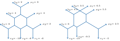
Figure 3: Left: The archetype of non-degenerate $(n=3)$-honeycombs as described in Section 4. The rays pointing in directions north west, north east and south have constant coordinates $\mathfrak{w}(h)_{i}=\lambda_{i}$, $\mathfrak{e}(h)_{i}=\mu_{i}$ and $\mathfrak{s}(h)_{i}=-\nu_{i}$, respectively. The remaining line segments contribute to the total edge length of the honeycomb. Right: A degenerate honeycomb, where the line segment at the top has been completely contracted. Here, only eight line segments remain to contribute to the total edge length.

The set $\mathrm{HONEY}_{n}$ of all $n$-honeycombs is identified as the closure of the set of non-degenerate ones, allowing edges of length zero as well. Thereby, $C=\{\mathrm{edge}(h)\mid h\in\mathrm{HONEY}_{n}\}\subset\mathbb{R}^{N}$ is a closed, convex, polyhedral cone.

Theorem 4.1 (Relation to honeycombs [23]).

The relation $\lambda\boxplus\mu\sim_{c}\nu$ is satisfied if and only if there exists a honeycomb $h$ with boundary values $\delta(h)=(\lambda,\mu,-\nu)$.

The set of triplets $\{(\lambda,\mu,-\nu)\in(\mathcal{D}^{n})^{3}\mid\lambda\boxplus\mu\sim_{c}\nu\}$ thus equals $\mathrm{BDRY}_{n}:=\{\delta(h)\mid h\in\mathrm{HONEY}_{n}\}$, which is at the same time the orthogonal projection of the cone $C$ to the coordinates associated with the boundary (the rays) — and, as shown in its verification, the very same cone described by the (in)equalities in Theorem 3.7.
There is also a related statement implicated by the ones in Lemma 3.9. If a triplet $(i,j,k)\in T_{r,n}$ yields an equality as in Eq. 3.3, then for the associated honeycomb $h$, $\delta(h)=(\lambda,\mu,-\nu)$, it holds

$$h=h_{1}\otimes h_{2},\quad\delta(h_{1})=(\lambda|_{i},\mu|_{j},-\nu|_{k}),\ \delta(h_{2})=(\lambda|_{i^{c}},\mu|_{j^{c}},-\nu|_{k^{c}}),$$ (4.1)

which means that $h$ is a literal overlay of two smaller honeycombs. Vice versa, if a honeycomb is an overlay of two smaller ones, then it yields two separate eigenvalue relations, however the splitting does not necessarily correspond to a triplet in $T_{r,n}$ [23].

Hives and feasibility of pairs

Definition 4.2 (Positive semi-definite honeycomb).

We define a positive semi-definite honeycomb $h$ as a honeycomb with boundary values $\mathfrak{w}(h),\mathfrak{e}(h)\geq 0$ and $\mathfrak{s}(h)\leq 0$.

A honeycomb can connect three matrices. In order to connect $m$ matrices, chains or systems of honeycombs are put in relation to each other through their boundary values. Although the phrase hive has appeared before as similar object to honeycombs, to which we do not intend to refer here, we use it to emphasize that a collection of honeycombs is given. Considerations for simple chains of honeycombs (cf. Lemma 4.6) have also been made in [22, 24], but we need to rephrase these ideas for our own purposes.

Definition 4.3 (Hives).

Let $n,M\in\mathbb{N}$. We define a (pos. semi-definite) $(n,M)$-hive $H$ as a collection of $M$ (pos. semi-definite) $n$-honeycombs $h^{(1)},\ldots,h^{(M)}$.

Definition 4.4 (Structure of hives).

Let $H$ be an $(n,M)$-hive and $B:=\{(i,\mathfrak{b})\mid i=1,\ldots,M,\ \mathfrak{b}\in\{\mathfrak{w},\mathfrak{e},\mathfrak{s}\}\}$. Further, let $\sim_{S}\ \in B\times B$ be an equivalence relation. We say $H$ has structure $\sim_{S}$ if the following holds:
Provided $(i,\mathfrak{b})\sim_{S}(j,\mathfrak{p})$, then if both $\mathfrak{b}$ and $\mathfrak{p}$ or neither of them equal $\mathfrak{s}$, it holds $\mathfrak{b}(h^{(i)})=\mathfrak{p}(h^{(j)})$, or otherwise $\mathfrak{b}(h^{(i)})=-\mathfrak{p}(h^{(j)})$.

We define the hive set $\mathrm{HIVE}_{n,M}(\sim_{S})$ as set of all $(n,M)$-hives $H$ with structure $\sim_{S}$.

In order to specify a structure $\sim_{S}$, we will only list generating sets of equivalences (with respect to reflexivity, symmetry and transitivity).

Definition 4.5 (Boundary map of structured hives).

Let $H$ be an $(n,M)$-hive with structure $\sim_{S}$. Let further $P:=\{(i,\mathfrak{b})\mid|[(i,\mathfrak{b})]_{\sim_{S}}|=1\}$ be the set of singletons. We define the boundary map $\delta_{P}:\mathrm{HIVE}_{n,M}(\sim_{S})\rightarrow(\mathcal{D}^{n})^{P}$ to map any hive $H\in\mathrm{HIVE}_{n,M}(\sim_{S})$ to the function $f_{P}:P\rightarrow\mathcal{D}^{n}$ defined via:
For all $(i,\mathfrak{b})\in P$, if $\mathfrak{b}$ equals $\mathfrak{s}$, it holds $f_{P}(i,\mathfrak{b})=-\mathfrak{b}(h^{(i)})$, or otherwise $f_{P}(i,\mathfrak{b})=\mathfrak{b}(h^{(i)})$.

A single $n$-honeycomb $h$ with boundary values $(\lambda,\mu,-\nu)$ can hence be identified as $(n,1)$-hive $H$ with trivial structure $\sim_{S}$ generated by the empty set, singleton set $P=\{(1,\mathfrak{w}),(1,\mathfrak{e}),(1,\mathfrak{s})\}$ and boundary $\delta_{P}(H)=\{(1,\mathfrak{w})\mapsto\lambda,(1,\mathfrak{e})\mapsto\mu,(1,\mathfrak{s})\mapsto\nu\}$. In this sense, it holds $\mathrm{HONEY}_{n}\cong\mathrm{HIVE}_{n,1}(\emptyset)$ and we regard honeycombs as hives as well. Another example is illustrated in Fig. 4, where $\sim_{S}$ is generated by $(1,\mathfrak{s})\sim_{S}(2,\mathfrak{w})$ and $(2,\mathfrak{s})\sim_{S}(3,\mathfrak{w})$, such that the singeltons are $P=\{(1,\mathfrak{w}),(1,\mathfrak{e}),(2,\mathfrak{e}),(3,\mathfrak{e}),(3,\mathfrak{s})\}$.

Lemma 4.6 (Eigenvalues of a sums of matrices).

The relation
$a^{(1)}\boxplus\ldots\boxplus a^{(m)}\sim_{c}c$ is satisfied if and only if there exists a hive $H$ of size $M=m-1$ (cf. Fig. 4) with structure $\sim_{S}$, generated by $(i,\mathfrak{s})\sim_{S}(i+1,\mathfrak{w})$, $i=1,\ldots,M-1$, and $\delta_{P}(H)=\{(1,\mathfrak{w})\mapsto a^{(1)},(1,\mathfrak{e})\mapsto a^{(2)},(2,\mathfrak{e})\mapsto a^{(3)},\ldots,(M,\mathfrak{e})\mapsto a^{(m)},(M,\mathfrak{s})\mapsto c\}$.

Proof.

“$\Rightarrow$”: The relation $a^{(1)}\boxplus\ldots\boxplus a^{(m)}\sim_{c}c$ is equivalent to the existence of Hermitian (or real symmetric, cf. Theorem 3.6) matrices $A^{(1)},\ldots,A^{(m)}$, $C=A^{(1)}+\ldots+A^{(m)}$ with eigenvalues $a^{(1)},\ldots,a^{(m)},c$, respectively. For $A^{(1,\ldots,k+1)}:=A^{(1,\ldots,k)}+A^{(k+1)},\ k=1,\ldots,m-1$, with accordant eigenvalues $a^{(1,\ldots,k)}$, the relation can equivalently be restated as $a^{(1,\ldots,k)}\boxplus a^{(k+1)}\sim_{c}a^{(1,\ldots,k+1)},\ k=1,\ldots,m-1$. This in turn is equivalent to the existence of honeycombs $h^{(1)},\ldots,h^{(m-1)}$ with boundary values $\delta(h^{(1)})=(a^{(1)},a^{(2)},-a^{(1,2)}),\delta(h^{(2)})=(a^{(1,2)},a^{(3)},-a^{(1,2,3)}),\ldots$, $\delta(h^{(m-1)})=(a^{(1,\ldots,m-1)},a^{(m)},-c)$. This depicts the structure $\sim_{S}$ and boundary function $\delta_{P}(H)$.
“$\Leftarrow$”: If in reverse the hive $H$ is assumed to exist, then we know, via the single honeycombs, that there exist matrices $\widetilde{A}^{(1,\ldots,k+1)}=A^{(1,\ldots,k)}+A^{(k+1)},\ k=1,\ldots,m-1$ with corresponding eigenvalues. Although we only know that $\widetilde{A}^{(1,\ldots,k+1)}$ and $A^{(1,\ldots,k+1)}$ share eigenvalues, the remaining, reverse construction is done via an inductive diagonalization argument (cf. Remark 2.11). ∎

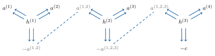
Figure 4: The schematic display of an $(n,3)$-hive $H$ with structure $\sim_{S}$ as in Lemma 4.6. North west, north east and south rays correspond to the boundary values $\mathfrak{w}(h_{i})$, $\mathfrak{e}(h_{i})$ and $\mathfrak{s}(h_{i})$, respectively. Coupled boundaries are in gray and connected by dashed lines.

The idea behind honeycomb overlays (cf. Eq. 4.1) can be extended to hives as well:

Lemma 4.7 (Zero eigenvalues).

If the relation
$a^{(1)}\boxplus\ldots\boxplus a^{(m)}\sim_{c}c$ is satisfied for $a^{(i)}\in\mathcal{D}_{\geq 0}^{n}$, $i=1,\ldots,m$, and $c_{n}=0$, then $a^{(1)}_{n}=\ldots=a^{(m)}_{n}=0$ and already $a^{(1)}|_{\{1,\ldots,n-1\}}\boxplus\ldots\boxplus a^{(m)}|_{\{1,\ldots,n-1\}}\sim_{c}c|_{\{1,\ldots,n-1\}}$.

Proof.

The first statement follows by basic linear algebra, since $a^{(1)},\ldots,a^{(m)}$ are nonnegative. For the second part, Lemma 4.6 and Eq. 4.1 are used. Inductively, in each honeycomb of the corresponding hive $H$, a separate $1$-honeycomb with boundary values $(0,0,0)$ can be found. Hence, each honeycomb is an overlay of such a $1$-honeycomb and an $(n-1)$-honeycomb. All remaining $(n-1)$-honeycombs then form a new hive with identical structure $\sim_{S}$. ∎

We arrive at an extended version of Theorem 2.10.

Theorem 4.8 (Equivalence to existence of a hive).

Let $(\gamma,\theta)\in\mathcal{D}^{\infty}_{\geq 0}\times\mathcal{D}^{\infty}_{\geq 0}$ and $n\geq\operatorname{deg}(\gamma),\operatorname{deg}(\theta)$. Further, let $\widetilde{\theta}=(\theta_{+},0,\ldots,0)$, $\widetilde{\gamma}=(\gamma_{+},0,\ldots,0)$ be $n$-tuples. The following statements are equivalent, independent of the choice $\mathbb{K}\in\{\mathbb{R},\mathbb{C}\}$:

• The pair $(\gamma,\theta)$ is feasible for $m\in\mathbb{N}$

• There are $m$ pairs of Hermitian, positive semi-definite matrices $(A^{(i)},B^{(i)})\in\mathbb{C}^{n\times n}\times\mathbb{C}^{n\times n}$, each with identical (multiplicities of) eigenvalues, such that $A:=\sum_{i=1}^{m}A^{(i)}$ has eigenvalues $\widetilde{\theta}^{2}$ and $B:=\sum_{i=1}^{m}B^{(i)}$ has eigenvalues $\widetilde{\gamma}^{2}$, respectively.

• There exist $a^{(1)},\ldots,a^{(m)}\in\mathcal{D}_{\geq 0}^{n}$ such that $a^{(1)}\boxplus\ldots\boxplus a^{(m)}\sim_{c}\widetilde{\gamma}^{2}$ as well as $a^{(1)}\boxplus\ldots\boxplus a^{(m)}\sim_{c}\widetilde{\theta}^{2}$.

• There exists a positive semi-definite $(n,M)$-hive $H$ of size $M=2(m-1)$ (cf. Fig. 5) with structure $\sim_{S}$, where $(i+u,\mathfrak{s})\sim_{S}(i+1+u,\mathfrak{w})$, $i=1,\ldots,M/2-1$, $u\in\{0,M/2\}$, as well as $(1,\mathfrak{w})\sim_{S}(1+M/2,\mathfrak{w})$ and $(i,\mathfrak{e})\sim_{S}(i+M/2,\mathfrak{e})$, $i=1,\ldots,M$. Further, $\delta_{P}(H)=\{(M/2,\mathfrak{s})\mapsto\widetilde{\gamma}^{2},(M,\mathfrak{s})\mapsto\widetilde{\theta}^{2}\}$.

Proof.

The existence of matrices with actual size $\operatorname{deg}(\gamma)$, $\operatorname{deg}(\theta)$, respectively, follows by repeated application of Lemma 4.7. The hive essentially consists of two rows of honeycombs as in Lemma 4.6. Therefor, the same argumentation holds, but instead of prescribed boundary values $a^{(i)}$, these values are coupled between the two hive parts. Due to Theorem 3.6, there is no difference whether we consider real or complex matrices and tensors. ∎

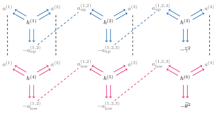
Figure 5: The schematic display of an $(n,6)$-hive $H$ (upper part in blue, lower part in magenta) with structure $\sim_{S}$ as in Lemma 4.6. North west, north east and south rays correspond to the boundary values $\mathfrak{w}(h_{i})$, $\mathfrak{e}(h_{i})$ and $\mathfrak{s}(h_{i})$, respectively. Coupled boundaries are in gray and connected by dashed lines.

The feasibility of $(\gamma,\theta)$ as in Eq. 3.1 is provided by the hive in Fig. 6. Even though not diagonally feasible, the pair can be disassembled, as later shown in Section 5.2, into multiple, diagonally feasible pairs, which then as well prove its feasibility.

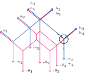
Figure 6: A $(4,2)$-hive consisting of two coupled honeycombs (blue for $\gamma$, magenta for $\theta$), which are slightly shifted for better visibility, generated by Algorithm 1. Note that some lines have multiplicity $2$. The coupled boundary values are given by $a=(4,1.5,0,0)$ and $b=(3.5,3.5,0,0)$. It proves the feasibility of the pair $(\gamma,\theta)$, $\widetilde{\gamma}^{2}=(7.5,5,0,0)$, $\widetilde{\theta}^{2}=(6,3.5,2,1)$ for $m=2$, since $\widetilde{\gamma}^{2},\widetilde{\theta}^{2}\sim_{c}a\boxplus b$ (the exponent ² has been skipped for better readability). Only due to the short, vertical line segment in the middle, the hive does not provide diagonal feasibility.

As another example serves $\gamma_{+}^{2}=(10,2,1,0.25,0.25)$ and $\theta_{+}^{2}=(4,3,2.5,2,2)$. According to (1.7), the pair $(\gamma,\theta)$ is not feasible for $m=2,3$, but may be feasible for $m=4$. The hive in Figs. 7 and 8 (having been constructed with Algorithm 1) provides that this is indeed the case. We further know that the pair is diagonally feasible for $m=5$ (due the constructive Theorem 3.4).

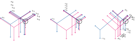
Figure 7: A $(5,4)$-hive consisting of six coupled honeycombs (blue for $\gamma$, magenta for $\theta$), which are slightly shifted for better visibility, generated by Algorithm 1. Note that some lines have multiplicity larger than $1$. Also, in each second pair of honeycombs, the roles of boundaries $\lambda$ and $\mu$ have been switched (which we can do due to the symmetry regarding $\boxplus$), such that the honeycombs can be combined to a single diagram as in Fig. 8. This means that the south rays of an odd numbered pair are always connected to the north-east (instead of north-west) rays of the consecutive pair. The boundary values are given by $a=(2,0.25,0.25,0,0)$, $b=(1,1,0.25,0,0)$, $c=(4,0,0,0,0)$ and $d=(3,1,0.75,0,0)$. It proves the feasibility of the pair $(\gamma,\theta)$, $\widetilde{\gamma}^{2}=(10,2,1,0.25,0.25)$, $\widetilde{\theta}^{2}=(4,3,2.5,2,2)$ for $m=4$, since both $\widetilde{\gamma}^{2},\widetilde{\theta}^{2}\sim_{c}a\boxplus b\boxplus c\boxplus d$ (the exponent ² has been skipped for better readability).

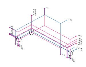
Figure 8: The three overlayed honeycomb pairs in Fig. 7 put together with respect to their coupling (the exponent ² for $\gamma,\theta$ has been skipped for better readability).

Hives are polyhedral cones

As previously done for honeycombs, we also associate hives with certain vector spaces.

Definition 4.9 (Hive sets and edge image).

Let $H$ be an $(n,M)$-hive consisting of honeycombs $h^{(1)},\ldots,h^{(M)}$. We define

$$\mathrm{edge}(H)=(\mathrm{edge}(h^{(1)}),\ldots,\mathrm{edge}(h^{(M)}))\in\mathbb{R}^{N\times M}$$

as the collection of constant coordinates of all edges appearing in the honeycombs within the hive $H$. Although defined via the abstract set $B$ (in Definition 4.3), we let $\sim_{S}$ act on the related edge coordinates as well. For $H\in\mathrm{HIVE}_{n,M}(\sim_{S})$, we then define the edge image as $\mathrm{edge}_{S}(H)\in{\raisebox{1.99997pt}{$\mathbb{R}^{N\times M}$}\left/\raisebox{-1.99997pt}{$\sim_{S}$}\right.}\cong\mathbb{R}^{N^{\ast}}$, in which coupled boundaries are assigned the same coordinate.

Theorem 4.10 (Hive sets are described by polyhedral cones).

• The hive set $\mathrm{HIVE}_{n,M}(\sim_{S})$, is a closed, convex, polyhedral cone, i.e. there exist matrices $L_{1},L_{2}$ s.t. $\mathrm{edge}_{S}(\mathrm{HIVE}_{n,M}(\sim_{S}))=\{x\mid L_{1}x\leq 0,\ L_{2}x=0\}$.

• Each fiber of $\delta_{P}$ (i.e. a set of hives with structure $\sim_{S}$ and boundary $f_{P}$), forms a closed, convex polyhedron, i.e. there exist matrices $L_{1},L_{2},L_{3}$ and a vector $b$ s.t. $\mathrm{edge}_{S}(\delta_{P}^{-1}(f_{P}))=\{x\mid L_{1}x\leq 0,\ L_{2}x=0,\ L_{3}x=b\}$.

Proof.

Each honeycomb of a hive follows its linear constraints. The hive structure and identification of coordinates as one and the same by $\sim_{S}$ only imposes additional linear constraints. The rest is elementary geometry. ∎

Corollary 4.11.

The boundary set

$$\mathrm{BDRY}_{n,M}(\sim_{S}):=\{\mathrm{image}(f_{P})\in(\mathcal{D}^{n})^{P}\mid f_{P}=\delta_{P}(H),\ H\in\mathrm{HIVE}_{n,M}(\sim_{S})\}$$

forms a closed, convex, polyhedral cone. This hence also holds for any intersection with, or projection to a lower dimensional subspace.

Proof.

The boundary set is given by the projection of $\mathrm{edge}_{S}(\mathrm{HIVE}_{n,M}(\sim_{S}))$ to the subset of coordinates associated to the ones in $P$. The proof is finished, since projections to fewer coordinates of closed, convex, polyhedral cones are again such cones. The same holds for intersections with subspaces. ∎

Cones of squared feasible values

The following fact has already been established in [4], but also follows from the previous Corollary 4.11.

Corollary 5.1 (Squared feasible pairs form cones).

Let $m,r_{1},r_{2}\in\mathbb{N}$. The set of squared feasible pairs $\mathcal{F}^{2}_{m,(r_{1},r_{2})}$ (cf. Definition 3.3) is a closed, convex, polyhedral cone, embedded into $\mathbb{R}^{r_{1}+r_{2}}$. If $r_{1}\leq mr_{2}$ and $r_{2}\leq mr_{1}$, then its dimension is $r_{1}+r_{2}-1$. Otherwise, $\mathcal{F}^{2}_{n,(r_{1},r_{2})}\cap\mathcal{D}^{r_{1}}_{>0}\times\mathcal{D}^{r_{2}}_{>0}$ is empty.

Proof.

By Corollary 4.11 and Theorem 4.8 it directly follows that $\mathcal{F}^{2}_{m,(r_{1},r_{2})}$ is a closed, convex, polyhedral cone. For the first case, it only remains to show that the cone has dimension $r_{1}+r_{2}-1$, or equivalently, it contains as many linearly independent vectors. These are however already given by the examples carried out in Lemma 3.2. From Corollary 2.8, it directly follows that if $(\gamma,\theta)$ is feasible for $m$, then it must hold $\operatorname{deg}(\gamma)\leq m\operatorname{deg}(\theta)$ and $\operatorname{deg}(\theta)\leq m\operatorname{deg}(\gamma)$, which provides the second case. ∎

The implication for the original TT-feasibility then is:

Corollary 5.2 (Cone property for higher order tensors).

For $d\in\mathbb{N}$, let both $\sigma,\tau\in(\mathcal{D}^{\infty}_{\geq 0})^{d-1}$ be feasible for $n\in\mathbb{N}^{d}$ (in the sense of Definition 1.1). Then $\upsilon$, $(\upsilon^{(\mu)})^{2}:=(\sigma^{(\mu)})^{2}+(\tau^{(\mu)})^{2}$, $\mu=1,\ldots,d-1$, is feasible for $n$ as well.

More general, squared feasible TT-singular values form a closed, convex, polyhedral cone. Its H-description is the collection of linear constraints for the pairs $(\sigma^{(\mu-1)},\sigma^{(\mu)})$.

Proof.

Due to Corollary 2.9, it only remains to show that each pair $(\upsilon^{(\mu-1)},\upsilon^{(\mu)})$ is feasible for $n_{\mu}$, $\mu=1,\ldots,d$. For each single $\mu$, this follows directly from Corollary 5.1.∎

Necessary inequalities

While for each specific $m$ and $r_{1}$, the results in [4] allow to calculate the $H$-description of the cone $\mathcal{F}^{2}_{m,(r_{1},mr_{1})}$ (i.e. a set of necessary and sufficient inequalities), we will concern ourselves with possibly weaker, but generalized statements for arbitrary $m$ in this section. In the subsequent Section 5.2, we will derive a $V$-description of $\mathcal{F}^{2}_{m,(m,m^{2})}$ (i.e. a set of generating vertices).

Lemma 5.3.

For $n,m\in\mathbb{N}$, let $T^{(j)}$, $I^{(j)}\subset\{1,\ldots,n\}$ be sets of equal cardinality, $j=1,\ldots,m$, with $T^{(1)}=I^{(1)}$ and $\Delta T^{(j)}\sim_{c}\Delta T^{(j-1)}\boxplus\Delta I^{(j)}$ (cf. Theorem 3.8) for $j=2,\ldots,m$. Then provided $\zeta\sim_{c}a^{(1)}\boxplus\ldots\boxplus a^{(m)}$, the inequality

$$\sum_{i\in T^{(m)}}\zeta_{i} \leq\sum_{j=1}^{m}\sum_{i\in I^{(j)}}a^{(j)}_{i}$$ (5.1)

holds true, for every $a^{(j)},\zeta\in\mathcal{D}^{n}$, $j=1,\ldots,m$. If Eq. 5.1 holds as equality, then already $\zeta|_{T^{(m)}}\sim_{c}a^{(1)}|_{I^{(1)}}\boxplus\ldots\boxplus a^{(m)}|_{I^{(m)}}$ and $\zeta|_{(T^{(m)})^{c}}\sim_{c}a^{(1)}|_{(I^{(1)})^{c}}\boxplus\ldots\boxplus a^{(m)}|_{(I^{(m)})^{c}}$. (cf. Lemma 3.9).

Proof.

The statement Eq. 5.1 follows inductively, if for each $j=2,\ldots,m$,

$$\sum_{i\in T^{(j)}}\nu_{i} \leq\sum_{i\in T^{(j-1)}}\lambda_{i}+\sum_{i\in I^{(j)}}\mu_{i}$$ (5.2)

is true whenever $\nu\sim_{c}\lambda\boxplus\mu$. By Theorem 3.8, this holds since by assumption $\Delta T^{(j)}\sim_{c}\Delta T^{(j-1)}\boxplus\Delta I^{(j)}$ for $j=2,\ldots,m$. If Eq. 5.1 holds as equality, then all single inequalities Eq. 5.2 must hold as equality, and hence Lemma 3.9 can be applied inductively as well. ∎

Theorem 5.4.

In the situation of Lemma 5.3, let $\widehat{T}$ and $\widehat{I}$ fulfill the same assumptions as $T$ and $I$. Let further $I^{(j)}\cap\widehat{I}^{(j)}=\emptyset$, $j=1,\ldots,m$. If the pair $(\gamma,\theta)\in\mathcal{D}^{\infty}_{\geq 0}\times\mathcal{D}^{\infty}_{\geq 0}$ is feasible for $m$, then

$$\sum_{i\in T^{(m)}}\gamma^{2}_{i}\leq\sum_{i\in\{1,\ldots,\operatorname{deg}(\theta)\}\setminus\widehat{T}^{(m)}}\theta^{2}_{i}$$ (5.3)

must hold true. If Eq. 5.3 holds as equality, then $((\gamma|_{T^{(m)}},0,\ldots),\ (\theta|_{(\widehat{T}^{(m)})^{c}},0,\ldots))$ and $((\gamma|_{(T^{(m)})^{c}},0,\ldots),\ (\theta|_{\widehat{T}^{(m)}},0,\ldots))$ are already feasible.

Together with Eq. 4.1 this also implies that the corresponding hive is an overlay of two smaller hives modulo zero boundaries.

Proof.

Let $n\geq\max(T^{(m)}),\operatorname{deg}(\gamma),\operatorname{deg}(\theta)$. As $(\gamma,\theta)$ is feasible, due to Lemma 5.3, the inequality Eq. 5.1 holds for some joint eigenvalues $a^{(1)},\ldots,a^{(m)}\in\mathcal{D}^{n}_{\geq 0}$ for both $\zeta:=\widetilde{\gamma}^{2}=(\gamma_{1}^{2},\ldots,\gamma_{n}^{2})$, $T$, $I$ and $\widehat{\zeta}=\widetilde{\theta}^{2}:=(\theta_{1}^{2},\ldots,\theta_{n}^{2})$, $\widehat{T}$, $\widehat{I}$. Furthermore, we have $\sum_{i=1}^{n}\theta_{i}^{2}=\sum_{i=1}^{n}a^{(1)}_{i}+\ldots+\sum_{i=1}^{n}a^{(m)}_{i}$. Subtracting Eq. 5.1 for $\widehat{\zeta}$ from this equality yields

$$\sum_{i\notin\widehat{T}^{(m)}}\theta^{2}_{i}\overset{n\geq\operatorname{deg}(\theta)}{=}\sum_{i\in\{1,\ldots,n\}\setminus\widehat{T}^{(m)}}\theta^{2}_{i} \overset{\lx@cref{creftype~refnum}{eq:necineq}\mbox{ for }\widehat{\zeta}}{\geq}\sum_{j=1}^{m}\sum_{i\in\{1,\ldots,n\}\setminus\widehat{I}^{(j)}}a^{(j)}_{i}$$ (5.4)

$$\overset{a_{i}^{(j)}\geq 0}{\geq}\sum_{j=1}^{m}\sum_{i\in I^{(j)}}a^{(j)}_{i}\overset{\lx@cref{creftype~refnum}{eq:necineq}\mbox{ for }\zeta}{\geq}\sum_{i\in T^{(m)}}\gamma^{2}_{i}.$$ (5.5)

This finishes the first part. In case of an equality, since the second “$\geq$” must hold as equality, we have $a^{(j)}|_{\{1,\ldots,n\}\setminus\widehat{I}^{(j)}}=(a^{(j)}|_{I^{(j)}},0,\ldots)$ and $a^{(j)}|_{\{1,\ldots,n\}\setminus I^{(j)}}=(a^{(j)}|_{\widehat{I}^{(j)}},0,\ldots)$ for each $j=1,\ldots,m$. Furthermore, the first and third “$\geq$” in Eq. 5.5 must hold as equality as well. Hence, the latter statement in Lemma 5.3 can be applied to the inequalities Eq. 5.1 for both $\zeta$ and $\widehat{\zeta}$, such that we can conclude the latter statement in this corollary. ∎

Corollary 5.5 (A set of inequalities for feasible pairs).

Let $p^{(1)}\ \dot{\cup}\ p^{(2)}=\mathbb{N}$ be two disjoint sets, with $p^{(1)}$ finite of size $r$. If $(\gamma,\theta)\in\mathcal{D}^{\infty}_{\geq 0}\times\mathcal{D}^{\infty}_{\geq 0}$ is feasible for $m\in\mathbb{N}$, then it holds ($p^{(u)}_{i}$ being the $i$-th smallest element)

$$\sum_{i\in P_{m}^{(1)}}\gamma^{2}_{i}\leq\sum_{i\notin P_{m}^{(2)}}\theta^{2}_{i},\quad P_{m}^{(u)}:=\{m(p^{(u)}_{i}-i)+i\mid i=1,2,\ldots\},\ u=1,2.$$

Proof.

Let $n\geq\max(P_{m}^{(1)}),\operatorname{deg}(\gamma),\operatorname{deg}(\theta)$. Let further $\widetilde{P}_{j}^{(2)}$ contain the $\widehat{k}$ smallest elements of $P_{j}^{(2)}$, where $\widehat{k}$ is the number of elements in $P_{m}^{(2)}\cap\{1,\ldots,n\}$, and let $\widetilde{P}_{j}^{(1)}=P_{j}^{(1)}$, $j=1,\ldots,m$. Thereby $\widetilde{P}_{1}^{(1)}=p^{(1)}=P_{1}^{(1)}$ and $\widetilde{P}_{1}^{(2)}\subset p^{(2)}=P_{1}^{(2)}$. We have the following (diagonal) matrix identities

$$\operatorname{diag}(\widetilde{P}_{j}^{(u)})-\operatorname{diag}(1,\ldots,\ell) =\operatorname{diag}(\widetilde{P}_{j-1}^{(u)})+\operatorname{diag}(\widetilde{P}_{1}^{(u)})-2\operatorname{diag}(1,\ldots,\ell)$$

$$\Leftrightarrow j(p^{(u)}_{i}-i) =(j-1)(p^{(u)}_{i}-i)+(p^{(u)}_{i}-i),\quad i=1,\ldots,\ell,\ \ell=|\widetilde{P}_{j}^{(u)}|$$

where the diagonal elements are placed in ascending order. Hence, $\bigtriangleup\widetilde{P}_{j}^{(u)}\sim_{c}\bigtriangleup\widetilde{P}_{j-1}^{(u)}\boxplus\bigtriangleup\widetilde{P}_{1}^{(u)}$ for $j=2,\ldots,m$, $u\in\{1,2\}$. For $T^{(j)}:=\widetilde{P}_{j}^{(1)}$, $I^{(j)}:=\widetilde{P}_{1}^{(1)}$ and $\widehat{T}^{(j)}:=\widetilde{P}_{j}^{(2)}$, $\widehat{I}^{(j)}:=\widetilde{P}_{1}^{(2)}$, we can apply Theorem 5.4 to obtain the desired statement. ∎

Among the various inequalities contained in Corollary 5.5, the following two correspond to early mentioned inequalities for Weyl’s problem. The first case is Eq. 1.7 and is also referred to as the basic inequalities in [4].

Corollary 5.6 (Ky Fan analogue for feas. pairs).

The choice $a^{(1)}=\{1,\ldots,r\}$ in Corollary 5.5 yields the inequality $\sum_{i=1}^{r}\gamma_{i}^{2}\leq\sum_{i=1}^{mr}\theta_{i}^{2}.$

Corollary 5.7 (Weyl analogue for feas. pairs).

The choice $a^{(1)}=\{r+1\}$ in Corollary 5.5 yields the inequality $\gamma_{rm+1}^{2}\leq\sum_{i=r+1}^{r+m}\theta_{i}^{2}.$

The QMP article [4] explicitly provides the derivation for the case $\operatorname{deg}(\gamma)\leq 3$ and $m=2$. Thereby, the necessary (and sufficient) inequalities for the feasibility of $(\gamma,\theta)$, apart from the trace property, are as follows: Corollary 5.6 for $r=1,2$; Corollary 5.7 for $r=1$ and $\gamma^{2}_{2}+\gamma^{2}_{3}\leq\theta^{2}_{1}+\theta^{2}_{2}+\theta^{2}_{3}+\theta^{2}_{6}$. The last inequality is not included in Corollary 5.5, but can be derived from Theorem 5.4 and be generalized in different ways. For example, for $I^{(1)}=I^{(2)}=\{1,3\}$, $T^{(2)}=\{2,3\}$, $\widehat{I}^{(1)}=\widehat{I}^{(2)}=\{2,4,5,6,\ldots\}$, $\widehat{T}^{(2)}=\{4,5,7,8,\ldots\}$ and $I^{(j)}=\{1,2\}$, $T^{(j)}=\{2,3\}$, $\widehat{I}^{(j)}=\{3,4,5,6,\ldots\}$, $\widehat{T}^{(j)}=\{2j,2j+1,2j+3,2j+4,\ldots\}$, $j=3,\ldots,m$, (where we add the same amount of arbitrarily many consecutive numbers in $\widehat{I}^{(j)}$ and $\widehat{T}^{(j)}$) one can conclude that $\gamma^{2}_{2}+\gamma^{2}_{3}\leq\sum_{i=1}^{2m-1}\theta^{2}_{i}+\theta^{2}_{2m+2}$ whenever $(\gamma,\theta)$ is feasible for $m$. Theorem 5.4 does however not provide when this generalized inequality is redundant to other necessary ones.

The right sum in Corollary 5.5 has always $m$-times as many summands as the left sum. For these inequalities, it further holds $\sum_{i\notin P_{m}^{(2)}}i-\sum_{i\in P_{m}^{(1)}}i=\sum_{i=k+1}^{mk}i=\frac{k(m-1)((m+1)k+1)}{2}$, where $k=|P_{m}^{(1)}|$. We can however only conjecture that this holds in general for every inequality in the $H$-description of $\mathcal{F}^{2}_{m,(r_{1},mr_{1})}$.

Vertex description of $\mathcal{F}^{2}_{m,(m,m^{2})}$

We revisit the special case Eq. 1.7 and derive the vertex description of the corresponding cone $\mathcal{F}^{2}_{m,(m,m^{2})}$ (cf. Definition 3.3). In this section, for $a,b\in\mathbb{N}\cup\{0\}$, let therefor $({a}_{\#b})=(a,\ldots,a)\in\mathcal{D}^{b}_{\geq 0}$ (length $b$).

Lemma 5.8.

Let $\alpha,\beta,m\in\mathbb{N}$, $\beta\leq m$, $\alpha\leq\beta m$, $\gamma_{+}^{2}=({\alpha}_{\#\beta})$ and $\theta_{+}^{2}=({\beta}_{\#\alpha})$. Then $(\gamma,\theta)$ is feasible for $m$.

Proof.

We prove by induction over $m$. Without loss of generality, we may assume $\alpha>\beta$ by which $\alpha=k\beta+t$ for unique natural numbers $k<m,t<\beta$. Considering Remark 2.11, it suffices to show that for $\widetilde{\gamma}^{2}:=\gamma_{+}^{2}-(t,{\beta}_{\#\beta-1})=(k\beta,{(\alpha-\beta)}_{\#\beta-1})$ and $\widetilde{\theta}^{2}:=\theta_{+}^{2}-(0,\ldots,0,t,{\beta}_{\#\beta-1})=({\beta}_{\#\alpha-\beta},\beta-t,{0}_{\#\beta-1})$ the pair $((\widetilde{\gamma},0,\ldots),(\widetilde{\theta},0,\ldots))$ is feasible for $m-1$. In order to show this, we split $\widetilde{\gamma}=(\widetilde{\gamma}_{(1)},\widetilde{\gamma}_{(2)})$, $\widetilde{\theta}=(\widetilde{\theta}_{(1)},\widetilde{\theta}_{(2)})$ into two pairs $\widetilde{\gamma}^{2}_{(1)}:=(k\beta)$, $\widetilde{\gamma}^{2}_{(2)}:=({\beta}_{\#k})$ and $\widetilde{\theta}^{2}_{(1)}:=({(\alpha-\beta)}_{\#\beta-1},0,\ldots,0)$, $\widetilde{\theta}^{2}_{(2)}:=({\beta}_{\#v},\beta-t,0,\ldots,0)$ with $v=\alpha-\beta-k=(k-1)(\beta-1)+(t-1)$. We can then, considering overlays of honeycombs, treat both pairs independently. While $((\widetilde{\gamma}_{(1)},0,\ldots),(\widetilde{\theta}_{(1)},0,\ldots))$ is feasible for $k\leq m-1$, in the second case, $(\widetilde{\gamma}^{2}_{(2)},\widetilde{\theta}^{2}_{(2)})$ is a convex combination of $({(v+1)}_{\#\beta-1})$, $({(\beta-1)}_{\#v+1})$ and $({v}_{\#\beta-1})$, $({(\beta-1)}_{\#v})$. Since $\beta-1\leq m-1$ and $v\leq v+1\leq(m-1)(\beta-1)$, the proof is finished by induction. ∎

The following theorem has priorly been conjectured by [4] and proven by [26]. We prove it in a way which allows to identify all vertices as in Corollary 5.10.

Theorem 5.9.

Let $(\gamma,\theta)\in\mathcal{D}^{\infty}_{\geq 0}\times\mathcal{D}^{\infty}_{\geq 0}$ and $m\in\mathbb{N}$. If $\operatorname{deg}(\gamma)\leq m$ and if all Ky Fan inequalities (Corollary 5.6) as well as the trace property $\|\gamma\|_{2}=\|\theta\|_{2}$ hold, then the pair is feasible for $m$.

Proof.

Here, we denote the Ky Fan inequality (Corollary 5.6) for $r$ with $K_{r}$, and in case of an equality we say $E_{r}$ holds. Due to $K_{m}$, $\operatorname{deg}(\gamma)\leq m$ and the trace property, $E_{m}$ and $\operatorname{deg}(\theta)\leq m\operatorname{deg}(\gamma)$ must be true. For fixed $m$, we prove by induction over $\operatorname{deg}(\gamma)+\operatorname{deg}(\theta)$. Let $0\leq k<m$ be the largest number for which $E_{k}$ is fulfilled and let $\alpha=\operatorname{deg}(\theta)-mk$ as well as $\beta=\operatorname{deg}(\gamma)-k$. We define $(\widehat{\gamma}^{2}\mid\widehat{\theta}^{2}):=(\gamma_{+}^{2}\mid\theta_{+}^{2})-f\cdot({m\beta}_{\#k},\ {\alpha}_{\#\beta}\mid{\beta}_{\#mk},\ {\beta}_{\#\alpha})$, $f>0$. Then $E_{k}$ and $K_{j}$, $j<k$, are true for $(\widehat{\gamma}\mid\widehat{\theta})$ for all $f>0$. Further, as long as $K_{k+1}$ holds for $(\widehat{\gamma}\mid\widehat{\theta})$ (which it does for any $f>0$ if $k=m-1$), then due to $K_{k-1}$ and $E_{k}$ it follows that $\widehat{\gamma}_{k+1}\leq\widehat{\gamma}_{k}$. Hence, $f$ can be chosen such that $K_{i}$, $i=1,\ldots,m-1,$ and $(\widehat{\gamma}\mid\widehat{\theta})\in\mathcal{D}_{\geq 0}^{\beta}\times\mathcal{D}_{\geq 0}^{\alpha}$ as well as either $(i)$ $E_{j}$ for at least one $j$, $k<j<m$, or $(ii)$ $\widehat{\gamma}_{\beta}=0\vee\widehat{\theta}_{\alpha}=0$. In case of $(i)$, we can repeat the above construction for increased $k$ until $k=m-1$ and hence $(ii)$ remains the sole option. In that case, we are finished by induction. ∎

Corollary 5.10.

A complete vertex description of $\mathcal{F}_{m,(m,m^{2})}$ is given by

$$\mathcal{V}=\{ (\widetilde{\gamma},\widetilde{\theta})\in\mathcal{F}_{m,(m,m^{2})}\mid\widetilde{\gamma}_{+}^{2}=({m\beta}_{\#k},\ {\alpha}_{\#\beta}),\ \widetilde{\theta}_{+}^{2}=({\beta}_{\#mk},\ {\beta}_{\#\alpha}),$$

$$\quad k\in\{0,\ldots,m-\beta\},\ \alpha,\beta\in\mathbb{N},\ \beta\leq m,\ \alpha\leq\beta m;\ \mbox{and }k=0\mbox{ if }\alpha=\beta m\}$$

A short calculation shows that the number of vertices $|\mathcal{V}|$ is given by a polynomial with leading monomial $m^{4}/6$.

Proof.

The proof of Theorem 5.9 is constructive and decomposes a squared feasible pair into a convex combination of squared feasible pairs in $\mathcal{V}$. It hence remains to show that the elements of $\mathcal{V}$ are vertices. Given any two elements $v=v(k_{1},\alpha_{1},\beta_{1})$, $w=w(k_{2},\alpha_{2},\beta_{2})$, $v^{2},w^{2}\in\mathcal{V}$, let $y^{2}_{f}=v^{2}-f\cdot w^{2}$, $f>0$. For $y_{f}\in\mathcal{D}^{m}_{\geq 0}\times\mathcal{D}^{m^{2}}_{\geq 0}$ to be true, we must have $mk_{1}+\alpha_{1}=mk_{2}+\alpha_{2}$ as well as either $(i)$ $k_{1}=k_{2}$ and $\beta_{1}=\beta_{2}$ or $(ii)$ $k_{2}=0$ and $\beta_{1}+k_{1}=\beta_{2}$. In the second case, $y_{f}$ would violate $K_{k_{1}}$ if $k_{1}\neq 0$. If $y^{2}_{f}$ is again a convex combination of elements in $\mathcal{V}$, $y_{f}$ must be feasible. Due to the above, it then however follows that $v=w$, $y^{2}=(1-f)v^{2}$. In other words, $v^{2}$ can not be a convex combination of other elements in $\mathcal{V}$. ∎

For example, all $7$ vertices $v^{2}_{1},\ldots,v^{2}_{7}$ of $\mathcal{F}^{2}_{2,(2,4)}\ (m=2)$ are given through

$$\left[\begin{smallmatrix}1&1\\ 0&0\\ &0\\ &0\end{smallmatrix}\right],\left[\begin{smallmatrix}2&1\\ 0&1\\ &0\\ &0\end{smallmatrix}\right],\left[\begin{smallmatrix}1&2\\ 1&0\\ &0\\ &0\end{smallmatrix}\right],\left[\begin{smallmatrix}1&1\\ 1&1\\ &0\\ &0\end{smallmatrix}\right],\left[\begin{smallmatrix}2&1\\ 1&1\\ &1\\ &0\end{smallmatrix}\right],\left[\begin{smallmatrix}3&2\\ 3&2\\ &2\\ &0\end{smallmatrix}\right]\mbox{and}\left[\begin{smallmatrix}2&1\\ 2&1\\ &1\\ &1\end{smallmatrix}\right].$$

For $m=3$, we already have $27$ vertices. Although all these vertices happen to be diagonally feasible, this is not the case in general. For example, $({5}_{\#3}\mid{3}_{\#5},{0}_{\#4})\in\mathcal{F}^{2}_{3,(3,9)}$ is a vertex, but it is easy to show that it is not diagonally feasible. For $(\gamma,\theta)$ as in Eq. 3.1, $\gamma_{+}^{2}=(7.5,5)$, $\theta_{+}^{2}=(6,3.5,2,1)$, we have $(\gamma_{+},\theta_{+})=1.5v^{3}_{1}+0.5v^{3}_{2}+1.5v^{2}_{4}+v^{2}_{5}+v^{2}_{7}$.

TFP algorithms

Matlab implementations of algorithms mentioned in this work can be found under the name TT-feasibility-toolbox or directly at

https://git.rwth-aachen.de/sebastian.kraemer1/TT-feasibility-toolbox.

The description in Theorem 4.10 yields the straightforward Algorithm 1 to determine the minimal value $m$ for which some pair $(\gamma,\theta)\in\mathcal{D}^{\infty}_{\geq 0}\times\mathcal{D}^{\infty}_{\geq 0}$ is feasible. The summed up length of all (inner) edges is minimized, since then the algorithm tends to return a hive from which diagonal feasibility can be read off (cf. Lemma 3.2).

Algorithm 1 Linear programming check for feasibility

0:  $(\widetilde{\gamma},\widetilde{\theta})\in\mathcal{D}^{r}_{\geq 0}\times\mathcal{D}^{r}_{\geq 0}$ with $\|\widetilde{\gamma}\|_{2}=\|\widetilde{\theta}\|_{2}$ for some $r\in\mathbb{N}$

1:  for $m=2\ldots$ do

2:     as in Theorem 4.10, set $L$ such that $\mathrm{edge}_{S}(\delta_{P}^{-1}(f_{P}))=\{x\mid L_{1}x\leq 0,\ L_{2}x=0,\ L_{3}x=b\}$ for the hive $H$ as in Theorem 4.8

3:     use a linear programming algorithm to minimize $Fx$ subject to $x\in\mathrm{edge}_{S}(\delta_{P}^{-1}(f_{P}))$, where $F$ is the vector for which $Fx\in\mathbb{R}_{\geq 0}$ is the summed up length of all (inner) edges in $H$

4:     if no solution exists then

5:        continue with $m+1$

6:     else

7:        return  minimal number $m\in\mathbb{N}$ for which $(\gamma,\theta)$ is feasible and a corresponding $(r,2(m-1))$-hive $H$ with minimal total edge length

8:     end if

9:  end for

Algorithm 1 always terminates for at most $m=\max(\operatorname{deg}(\gamma),\operatorname{deg}(\theta))$ due to Lemma 3.2. In practice, a slightly different coupling of boundaries is used (cf. Fig. 7), since then the entire hive can be visualized in $\mathbb{R}^{2}$. For that, it is required to rotate and mirror some of the honeycombs (cf. Fig. 8). Depending on the linear programming algorithm, the input may be too badly conditioned to allow a verification with satisfying residual.

Algorithm 2 Heuristic check for numerical feasibility

0:  $(\gamma_{+},\theta_{+})\in\mathcal{D}^{r_{1}}_{>0}\times\mathcal{D}^{r_{2}}_{>0}$ for some $r_{1},r_{2}\in\mathbb{N}$ and a natural number $m$ (as well as $\mathrm{tol}>0$, $\mathrm{iter_{max}}>0$)

1:  initialize a core $H^{(1)}_{1}$ of length $m$ and size $(r_{1},r_{2})$ randomly

2:  set $\gamma^{(0)},\theta^{(0)}\equiv 0$, $\mathrm{relres}=1$ and $k=0$

3:  while $\mathrm{relres}>\mathrm{tol}$ and $k\leq\mathrm{iter_{max}}$ do

4:     $k=k+1$

5:     calculate the SVD and set $U_{1}\Theta^{(k)}V_{1}^{T}=\mathfrak{L}(H^{(k-1)}_{1})$

6:     set $H^{(k)}_{2}$ via $\mathfrak{L}(H^{(k)}_{2})=U_{1}\Theta$

7:     calculate the SVD and set $U_{2}\Gamma^{(k)}V_{2}^{T}=\mathfrak{R}(H^{(k)}_{2})$

8:     set $H^{(k)}_{1}$ via $\mathfrak{R}(H^{(k)}_{1})=\Gamma V_{2}^{T}$

9:     $\mathrm{relres}=\max\left(\max_{i=1,\ldots,r_{1}}(|\gamma^{(k)}_{i}/\gamma_{i}-1|),\max_{i=1,\ldots,r_{2}}(|\theta^{(k)}_{i}/\theta_{i}-1|)\right)$

10:  end while

11:  if $\mathrm{relerr}\leq\mathrm{tol}$ then

12:     return  $H^{\ast}=\Gamma^{-1}\ H_{1}^{(k)}\ \Theta^{-1}$

13:     $(\gamma,\theta)$ is (numerically) feasible for $m$

14:  else

15:     $(\gamma,\theta)$ is likely to not be feasible for $m$

16:  end if

The simple and heuristic Algorithm 2 can be more reliable. As we have seen, we can restrict ourselves to $\mathbb{K}=\mathbb{R}$ (cf. Theorem 3.6). Fixpoints of the iteration are cores $H\in(\mathbb{R}^{r_{1}\times r_{2}})^{\{1,\ldots,m\}}$ for which $H\Theta^{-1}$ is left-orthonormal and $\Gamma^{-1}H$ is right-orthonormal. Hence $H^{\ast}=\Gamma^{-1}\ H\ \Theta^{-1}$ is a core for which $\Gamma H^{\ast}$ is left-orthonormal and $H^{\ast}\Theta$ is right-orthonormal, as required by Corollary 2.8. Furthermore, the iterates cannot diverge in the following sense:

Lemma 6.1 (Behavior of Algorithm 2).

For every $k>1$ it holds $\|\gamma^{(k)}-\gamma_{+}\|_{2}\leq\|\theta^{(k)}-\theta_{+}\|_{2}$ as well as $\|\theta^{(k)}-\theta_{+}\|_{2}\leq\|\gamma^{(k-1)}-\gamma_{+}\|_{2}$.

Proof.

We only consider the first case, since the other one is analogous. Let $k>1$ be arbitrary, but fixed. Then in line $5$ of Algorithm 2 we have

$$\|\underbrace{U_{1}\Theta^{(k)}V_{1}^{T}}_{A:=}-\underbrace{U_{1}\Theta V_{1}^{T}}_{B:=}\|_{F}=\|\Theta^{(k)}-\Theta\|_{F}.$$

$\mathfrak{R}(A)$ has singular values $\gamma_{+}$, inherited from the last iteration and $\mathfrak{R}(B)$ has the same singular values as $\mathfrak{R}(B)\operatorname{diag}(V_{1},\ldots,V_{1})=\mathfrak{R}(BV_{1})=\mathfrak{R}(H_{2}^{(k)})$, which are given by $\gamma^{(k)}$. It follows by Mirsky’s inequality about singular values [27] that $\|\gamma^{(k)}-\gamma_{+}\|_{2}\leq\|A-B\|_{F}=\|\theta^{(k)}-\theta_{+}\|_{2}$. ∎

Convergence is hence not assured, but likely in the sense that the perturbation of matrices usually leads to a fractional amount of perturbation of its singular values. To construct an entire tensor, the algorithm may be run in parallel for each single core.

Conclusions and outlook

The simple equivalence between the tensor feasibility (TFP) and quantum marginal problem (QMP) allows for an interesting interaction between the different perspectives on either side. Through the standard representation, the tensor train (TT-)feasibility problem can be decoupled into pairwise problems, by which, firstly, results from the QMP can be applied. Thereby, the full H-description of the cone of squared TT-feasible values can be calculated in any specific instance. At the same time, through our alternative consideration of orthogonality constraints on cores, one can derive universal classes of necessary inequalities for the feasibility of pairs, whereas the concept of hives yields a corresponding linear programming algorithm. Further on the practical side, we have introduced simple ways to construct tensors with prescribed singular values in parallel, based only on the sufficient construction of feasible pairs. Given that the concept of a standard representation is transferable to any hierarchical format, implications for both the TFP and QMP are subject to future research.

References

- [1] A. Berenstein and R. Sjamaar, Coadjoint orbits, moment polytopes, and the Hilbert-Mumford criterion, Journal of the American Mathematical Society, 13 (2000), pp. 433–466, https://doi.org/10.1090/S0894-0347-00-00327-1.
- [2] R. Bhatia, Linear algebra to quantum cohomology: The story of Alfred Horn’s inequalities, The American Mathematical Monthly, 108 (2001), pp. 289–318, https://doi.org/10.2307/2695237.
- [3] A. Cichocki, D. Mandic, L. De Lathauwer, G. Zhou, Q. Zhao, C. Caiafa, and H. A. PHAN, Tensor decompositions for signal processing applications: From two-way to multiway component analysis, IEEE Signal Processing Magazine, 32 (2015), pp. 145–163, https://doi.org/10.1109/MSP.2013.2297439.
- [4] S. Daftuar and P. Hayden, Quantum state transformations and the Schubert calculus, Annals of Physics, 315 (2005), pp. 80 – 122, https://doi.org/10.1016/j.aop.2004.09.012. Special Issue.
- [5] L. De Lathauwer, B. De Moor, and J. Vandewalle, A multilinear singular value decomposition, SIAM Journal on Matrix Analysis and Applications, 21 (2000), pp. 1253–1278, https://doi.org/10.1137/S0895479896305696.
- [6] I. Domanov, A. Stegeman, and L. De Lathauwer, On the largest multilinear singular values of higher-order tensors, SIAM Journal on Matrix Analysis and Applications, 38 (2017), pp. 1434–1453, https://doi.org/10.1137/16M110770X.
- [7] K. Fan, On a theorem of Weyl concerning eigenvalues of linear transformations. i, Proceedings of the National Academy of Sciences of the United States of America, 35 (1949), pp. 652–655, https://doi.org/10.1073/pnas.35.11.652.
- [8] M. Franz, Moment polytopes of projective G‑varieties and tensor products of symmetric group representations, J. Lie Theory, 12 (2002), pp. 539–549.
- [9] S. Friedland, Finite and infinite dimensional generalizations of Klyachko’s theorem, Linear Algebra and its Applications, 319 (2000), pp. 3 – 22, https://doi.org/10.1016/S0024-3795(00)00217-2.
- [10] W. Fulton, Eigenvalues, invariant factors, highest weights, and Schubert calculus, Bull. Amer. Math. Soc. (N.S.), 37 (2000), pp. 209–249, https://doi.org/10.1090/S0273-0979-00-00865-X.
- [11] W. Fulton, Eigenvalues of majorized Hermitian matrices and LittlewoodâRichardson coefficients, Linear Algebra and its Applications, 319 (2000), pp. 23 – 36, https://doi.org/10.1016/S0024-3795(00)00218-4.
- [12] L. Grasedyck, Hierarchical singular value decomposition of tensors, SIAM Journal on Matrix Analysis and Applications, 31 (2010), pp. 2029–2054, https://doi.org/10.1137/090764189.
- [13] L. Grasedyck, D. Kressner, and C. Tobler, A literature survey of low-rank tensor approximation techniques, GAMM-Mitteilungen, 36 (2013), pp. 53–78, https://doi.org/10.1002/gamm.201310004.
- [14] W. Hackbusch, D. Kressner, and A. Uschmajew, Perturbation of higher-order singular values, SIAM Journal on Applied Algebra and Geometry, 1 (2017), pp. 374–387, https://doi.org/10.1137/16M1089873.
- [15] W. Hackbusch and A. Uschmajew, On the interconnection between the higher-order singular values of real tensors, Numerische Mathematik, 135 (2017), pp. 875–894, https://doi.org/10.1007/s00211-016-0819-9.
- [16] U. Helmke and J. Rosenthal, Eigenvalue inequalities and Schubert calculus, Mathematische Nachrichten, 171 (1995), pp. 207–225, https://doi.org/10.1002/mana.19951710113.
- [17] A. Higuchi, On the one-particle reduced density matrices of a pure three-qutrit quantum state, (2003), https://arxiv.org/abs/quant-ph/0309186v2.
- [18] A. Higuchi, A. Sudbery, and J. Szulc, One-qubit reduced states of a pure many-qubit state: Polygon inequalities, Phys. Rev. Lett., 90 (2003), p. 107902, https://doi.org/10.1103/PhysRevLett.90.107902.
- [19] A. Horn, Eigenvalues of sums of Hermitian matrices., Pacific J. Math., 12 (1962), pp. 225–241, http://projecteuclid.org/euclid.pjm/1103036720.
- [20] A. A. Klyachko, Stable bundles, representation theory and Hermitian operators, Selecta Math. (N.S.), 4 (1998), pp. 419–445, https://doi.org/10.1007/s000290050037.
- [21] A. A. Klyachko, Quantum marginal problem and N-representability, Journal of Physics: Conference Series, 36 (2006), pp. 72–86, https://doi.org/10.1088/1742-6596/36/1/014.
- [22] A. Knutson and T. Tao, The honeycomb model of tensor products. I. Proof of the saturation conjecture, J. Amer. Math. Soc., 12 (1999), pp. 1055–1090, https://doi.org/10.1090/S0894-0347-99-00299-4.
- [23] A. Knutson and T. Tao, Honeycombs and sums of Hermitian matrices, Notices Amer. Math. Soc., 48 (2001), pp. 175–186.
- [24] A. Knutson, T. Tao, and C. Woodward, The honeycomb model of tensor products. II. Puzzles determine facets of the Littlewood-Richardson cone, J. Amer. Math. Soc., 17 (2004), pp. 19–48, https://doi.org/10.1090/S0894-0347-03-00441-7.
- [25] T. G. Kolda and B. W. Bader, Tensor decompositions and applications, SIAM Review, 51 (2009), pp. 455–500, https://doi.org/10.1137/07070111X.
- [26] C.-K. Li, Y.-T. Poon, and X. Wang, Ranks and eigenvalues of states with prescribed reduced states, Electronic Journal of Linear Algebra, 27 (2014), https://doi.org/10.13001/1081-3810.2882.
- [27] L. Mirsky, Symmetric gauge functions and unitarily invariant norms, Quart. J. Math. Oxford Ser. (2), 11 (1960), pp. 50–59, https://doi.org/10.1093/qmath/11.1.50.
- [28] I. V. Oseledets, Tensor-train decomposition, SIAM Journal on Scientific Computing, 33 (2011), pp. 2295–2317, https://doi.org/10.1137/090752286.
- [29] C. Schilling, Quantum marginal problem and its physical relevance, PhD thesis, ETH Zurich, 2014, https://doi.org/10.3929/ethz-a-010139282. Diss., Eidgenössische Technische Hochschule ETH Zürich, Nr. 21748, 2014.
- [30] A. Seigal, Gram determinants of real binary tensors, Linear Algebra and its Applications, 544 (2018), pp. 350–369, https://doi.org/10.1016/j.laa.2018.01.019.
- [31] N. D. Sidiropoulos, L. De Lathauwer, X. Fu, K. Huang, E. E. Papalexakis, and C. Faloutsos, Tensor decomposition for signal processing and machine learning, IEEE Transactions on Signal Processing, 65 (2017), pp. 3551–3582, https://doi.org/10.1109/TSP.2017.2690524.
- [32] L. R. Tucker, Some mathematical notes on three-mode factor analysis, Psychometrika, 31 (1966), pp. 279–311, https://doi.org/10.1007/BF02289464.
- [33] G. Vidal, Efficient classical simulation of slightly entangled quantum computations, Phys. Rev. Lett., 91 (2003), p. 147902, https://doi.org/10.1103/PhysRevLett.91.147902.
- [34] H. Weyl, Das asymptotische Verteilungsgesetz der Eigenwerte linearer partieller Differentialgleichungen (mit einer Anwendung auf die Theorie der Hohlraumstrahlung), Mathematische Annalen, 71 (1912), pp. 441–479, https://doi.org/10.1007/BF01456804.