General relativistic magnetohydrodynamic simulations of binary neutron star mergers
forming a long-lived neutron star

Abstract

Merging binary neutron stars (BNSs) represent the ultimate targets for multimessenger astronomy, being among the most promising sources of gravitational waves (GWs), and, at the same time, likely accompanied by a variety of electromagnetic counterparts across the entire spectrum, possibly including short gamma-ray bursts (SGRBs) and kilonova/macronova transients. Numerical relativity simulations play a central role in the study of these events. In particular, given the importance of magnetic fields, various aspects of this investigation require general relativistic magnetohydrodynamics (GRMHD). So far, most GRMHD simulations focused the attention on BNS mergers leading to the formation of a hypermassive NS, which, in turn, collapses within few tens of ms into a black hole surrounded by an accretion disk. However, recent observations suggest that a significant fraction of these systems could form a long-lived NS remnant, which will either collapse on much longer timescales or remain indefinitely stable. Despite the profound implications for the evolution and the emission properties of the system, a detailed investigation of this alternative evolution channel is still missing. Here, we follow this direction and present a first detailed GRMHD study of BNS mergers forming a long-lived NS. We consider magnetized binaries with different mass ratios and equations of state and analyze the structure of the NS remnants, the rotation profiles, the accretion disks, the evolution and amplification of magnetic fields, and the ejection of matter. Moreover, we discuss the connection with the central engine of SGRBs and provide order-of-magnitude estimates for the kilonova/macronova signal. Finally, we study the GW emission, with particular attention to the post-merger phase.

I Introduction

With the discovery of binary black hole (BH) mergers by the Laser Interferometer Gravitational Wave Observatory (LIGO), the era of gravitational wave (GW) astronomy and multimessenger astronomy including GWs has begun Abbott et al. (2016a); Abbott and et al (2016b, b). As the advanced LIGO and Virgo detectors approach design sensitivity in the next few years LIGO Scientific Collaboration et al. (2015); Accadia et al. (2011), exciting new discoveries could be made, including binary neutron star (BNS) and NS–BH mergers Abadie et al. (2010); Abbott et al. (2016b). Due to the absence of baryonic matter in these systems, stellar-mass binary BH mergers are not expected to produce bright electromagnetic (EM) counterparts to their GW signal (but see, e.g., Perna et al. (2016)). Instead, mergers involving NSs are expected to link the EM and GW skies. Furthermore, these mergers are also of wide interest as they offer a unique opportunity to constrain the equation of state (EOS) of matter at supranuclear densities (e.g., Shibata et al. (2005); Bauswein et al. (2013)) and provide a prime candidate astrophysical site for the production of heavy elements in the universe, via r-process nucleosynthesis in the matter ejected during and possibly after merger (e.g., Just et al. (2015); Wu et al. (2016); Roberts et al. (2017)).

Mergers involving NSs are expected to generate EM emission across the entire EM spectrum and over a variety of timescales Metzger and Berger (2012). Detection of EM counterparts will enable the identification of the host galaxy and its position within/relative to the host, which will provide valuable information on binary formation channels, age of the stellar population, and supernova birth kicks Berger (2014). Additionally, by measuring redshifts, EM counterparts can determine the distance to the source and help alleviate degeneracies in the GW parameter estimation between distance and inclination of the binary. Moreover, combined GW and EM observations can prove the connection between short gamma-ray bursts (SGRBs) and BNS or NS-BH mergers (see below), revealing crucial information on when and how a SGRB can be produced. Finally, even without a GW detection, EM counterparts can reveal exclusive information on the very rich physics of the merger and post-merger evolution, especially if the merger remnant is a massive NS Metzger et al. (2014); Siegel and Ciolfi (2016a, b).

SGRBs are among the earliest proposed counterparts to BNS and NS-BH mergers Paczynski (1986); Eichler et al. (1989); Narayan et al. (1992); Barthelmy et al. (2005); Fox et al. (2005); Gehrels et al. (2005); Shibata et al. (2006); Tanvir et al. (2013); Berger et al. (2013); Paschalidis et al. (2015); Ruiz et al. (2016). The standard paradigm explains the formation of a SGRB via a relativistic outflow (jet) generated by a torus of matter accreting onto a remnant BH. Although there is tentative evidence for this scenario on the basis of previous general-relativisitc magnetohydrodynamic (GRMHD) simulations Paschalidis et al. (2015); Ruiz et al. (2016), much still remains to be understood. Moreover, if the merger leads to the formation of a long-lived NS instead of a BH, which, as we argue below, can occur in an order unity fraction of all BNS merger events (but not in NS-BH mergers), baryon pollution in the surrounding of the merger site Hotokezaka et al. (2013a); Oechslin et al. (2007); Bauswein et al. (2013); Kastaun and Galeazzi (2015); Dessart et al. (2009); Siegel et al. (2014); Metzger and Fernández (2014) can choke a relativistic outflow Murguia-Berthier et al. (2014); Nagakura et al. (2014); Murguia-Berthier et al. (2016) or even prevent its formation in the first place. Ref. Ciolfi and Siegel (2015a) has proposed the “time-reversal” scenario, in which the problem of baryon pollution can be avoided, with additional important observational consequences (see Rezzolla and Kumar (2015) for an alternative proposal). In order to explore the SGRB-merger connection for the BNS case, more simulations of systems with different properties are required, to examine in detail the merger and early post-merger dynamics and to better quantify the amount of baryon pollution and thus the potential for generating relativistic outflows. Furthermore, magnetic fields are likely to play a key role in the formation of a jet and therefore investigating the nature of SGRBs demands GRMHD simulations.

Kilonovae or macronovae represent another important EM counterpart to the GW signal of BNS and NS-BH mergers Li and Paczyński (1998); Kulkarni (2005); Rosswog (2005); Metzger et al. (2010); Roberts et al. (2011); Barnes and Kasen (2013); Piran et al. (2013); Tanvir et al. (2013); Berger et al. (2013); Yang et al. (2015). These thermal transients at optical and infrared wavelengths and timescales of days to weeks are powered by heating from radioactive decay of r-process elements produced in the expanding sub-relativistic ejecta. The amount of r-process material synthesized in the dynamical ejecta (e.g., Hotokezaka et al. (2013a); Oechslin et al. (2007); Bauswein et al. (2013); Kastaun and Galeazzi (2015); Radice et al. (2016)) and in winds from the remnant object Dessart et al. (2009); Siegel et al. (2014), or from a remnant accretion disk/torus Fernández and Metzger (2013); Just et al. (2015) depend sensitively on properties of the matter outflows at launch, such as the distributions in mass, velocity, entropy, and electron fraction. Numerical simulations are necessary to investigate these properties in detail.

Table 1: Initial data parameters: mass ratio ($q=M_{\mathrm{g}}^{1}/M_{\mathrm{g}}^{2}$), total baryonic mass of the system ($M_{\mathrm{b}}^{\mathrm{tot}}$), baryonic and gravitational masses of each star at infinite separation ($M_{\mathrm{b}}$ and $M_{\mathrm{g}}$), compactness ($M_{\mathrm{g}}/R_{c}$, dimensionless), initial orbital frequency and proper separation ($f_{0}$ and $d$), initial magnetic energy ($E_{\mathrm{mag}}$), initial maximum value of magnetic field strength ($B_{\mathrm{max}}$), and $A_{b}$, the value in geometric units used in equation (1) in order to fix $B_{\mathrm{max}}$.

Model	APR4 equal	APR4 unequal	MS1 equal	MS1 unequal	H4 equal	H4 unequal
$q$	$1$	$0.90$	$1$	$0.91$	$1$	$0.91$
$M_{\mathrm{b}}^{\mathrm{tot}}$ [$M_{\odot}$]	$2.98$	$2.98$	$2.91$	$2.91$	$2.92$	$2.92$
$M_{\mathrm{b}}$ [$M_{\odot}$]	$1.49$	$1.58,1.41$	$1.45$	$1.53,1.38$	$1.46$	$1.54,1.38$
$M_{\mathrm{g}}$ [$M_{\odot}$]	$1.35$	$1.42,1.28$	$1.35$	$1.41,1.28$	$1.35$	$1.42,1.29$
$M_{\mathrm{g}}/R_{c}$	$0.176$	$0.185,0.167$	$0.134$	$0.140,0.127$	$0.143$	$0.150,0.135$
$f_{0}$ [Hz]	$283$	$284$	$287$	$287$	$287$	$286$
$d$ [km]	$59$	$59$	$57$	$57$	$58$	$58$
$E_{\mathrm{mag}}$ [$10^{47}$erg]	$2.42$	$2.42$	$2.42$	$2.42$	$2.42$	$2.42$
$B_{\mathrm{max}}$ [$10^{15}$G]	$3.00$	$3.51,2.37$	$2.05$	$2.36,1.70$	$2.42$	$2.91,1.89$
$A_{b}$	$776$	$748$	$4714$	$4609$	$2816$	$2720$

While NS-BH mergers inevitably end up in a BH possibly surrounded by a massive accretion disk, BNS mergers can lead to qualitatively different remnants. Depending on the EOS and the component masses, the BNS can form a BH (prompt collapse), a hypermassive NS (HMNS; NS with mass above the maximum mass for uniformly rotating configurations), or a long-lived NS, which we assume to be either supramassive (SMNS; NS with mass above the maximum mass $M_{\mathrm{TOV}}$ for non-rotating configurations) or indefinitely stable. HMNSs typically collapse to a BH on a timescale of $\sim\!\text{ms}$ to $\sim\!100\,\text{ms}$, while SMNSs can typically survive for minutes or even much longer. It is commonly believed that HMNSs are supported against collapse by rapid rotation of the core (see Baumgarte et al. (2000) for such HMNS models) and consequently collapse when enough differential rotation is removed (via GW emission or electromagnetic torques Shibata and Taniguchi (2006); Duez et al. (2006a); Siegel et al. (2013)). SMNS are thought to be supported by uniform rotation and to collapse when enough angular momentum is carried away via magnetic dipole radiation and GWs. In contrast, a growing number of simulations Kastaun and Galeazzi (2015); Endrizzi et al. (2016); Kastaun et al. (2016a, b); Hanauske et al. (2016) indicate that both HMNSs and SMNSs typically have slowly rotating cores, and that collapse is rather avoided because a significant amount of matter in the outer layers approaches Kepler velocity. This implies that the exact mechanism leading to collapse is still poorly understood, which has important consequences when interpreting the lifetimes of HMNSs and SMNSs. Therefore, special attention should be paid to the rearrangement of the radial remnant structure preceding collapse.

BNS mergers leading to a hypermassive, supramassive or stable NS are characterized by a post-merger phase in which GW emission can still be significant for several tens of ms (or more) and in general much stronger than the short and weak BH ringdown signal. This post-merger GW emission carries the signature of the remnant structure and represents a promising way to constrain the NS EOS. In particular, the spectrum always shows a dominant peak at a frequency that strongly depends on the EOS (e.g., Bauswein and Janka (2012); Bauswein et al. (2014); Takami et al. (2014)).

In this paper, we perform a set of GRMHD simulations of BNS mergers with different EOS and mass ratios, focusing most of the attention on systems leading to the formation of a long-lived remnant NS (i.e. supramassive or stable). For comparison, we also consider two BNS mergers forming a HMNS that collapses to a BH by the end of the simulation. With $M_{\mathrm{TOV}}\gtrsim 2\,M_{\odot}$ Demorest et al. (2010); Antoniadis et al. (2013), the maximum mass of uniformly rotating configurations $\sim\!20\%$ larger, i.e. $M_{\mathrm{supra}}\approx 1.2\,M_{\mathrm{TOV}}\gtrsim 2.4\,M_{\odot}$ Lasota et al. (1996), and a typical remnant mass between $2.3-2.5\,M_{\odot}$ when accounting for mass loss and neutrino and GW emission Belczynski et al. (2008), we expect that an important (order unity) fraction of BNS merger events should lead to the formation of a long-lived NS. Despite being very likely, this case remains poorly studied in numerical relativity, and only a few simulations of such systems were performed including magnetic fields (i.e. in GRMHD) Giacomazzo and Perna (2013); Palenzuela et al. (2015); Endrizzi et al. (2016).

The presence of a long-lived remnant has important consequences. First, neutrino and/or magnetically driven outflows can provide an additional source of ejecta material for r-process nucleosynthesis on secular timescales ($\sim\!1\,\mathrm{s}$) Dessart et al. (2009); Siegel et al. (2014). Second, the spindown radiation from the magnetized remnant NS represents an additional source of energy that can power nearly isotropic EM transients. This emission provides a possible explanation for the long-lasting ($\sim$minutes to hours) X-ray afterglows observed by Swift Gehrels et al. (2004) in association with a substantial fraction of SGRB events Rowlinson et al. (2013); Lü et al. (2015). At the same time, long-lasting afterglows are hardly explained within the popular BH-disk scenario of SGRBs, due to the short accretion timescale of the disk onto the BH ($\sim$seconds). If the above interpretation is correct, this provides additional evidence that the product of BNS mergers is very often a long-lived NS. Moreover, independently from SGRBs, spindown-powered EM transients represent an additional and potentially very promising EM counterpart for multimessenger astronomy with BNS mergers Yu et al. (2013); Metzger et al. (2014); Siegel and Ciolfi (2016a, b). In addition, they may be connected with other astrophysical phenomena, such as fast radio bursts Dai et al. (2016).

Here, we initiate a systematic investigation on BNS mergers ending up in a long-lived NS, aimed at covering all of the key aspects mentioned above. The paper is organized as follows. Section II describes the physical models, the numerical setup and the generation of initial data. In Section III we discuss in detail the evolution from the inspiral to the post-merger phase for the different models. The following sections provide a more detailed analysis of individual aspects, such as the rotation profile of the remnant, its structure and its stability against collapse (Section IV), the evolution of magnetic fields (Section V), and the implications for SGRBs (Section VI). In Section VII we investigate mass ejection, while Section VIII is devoted to the analysis of the GW emission, with particular emphasis on the post-merger signal. Conclusions are presented in Section IX and an appendix is added to discuss aspects of numerical convergence.

II Physical models and numerical setup

In this work, we study a set of magnetized BNS systems with a mass ratio of either $q=1$ (equal mass) or $q=0.9$ (unequal mass). The most relevant initial parameters of our models are summarized in Table 1. In the equal-mass case, each NS has a gravitational mass at infinite separation of $1.35$ M_⊙, which appears to be the most likely mass for NSs in a merging BNS system according to current models and observations (e.g., Belczynski et al. (2008); Lattimer (2012); Özel and Freire (2016)). For the unequal-mass case ($q=0.9$), we impose the same total gravitational mass at infinite separation. Both the individual masses and the mass ratios we consider span roughly the same range as the available BNS observations with well constrained masses Lattimer (2012); Özel and Freire (2016). We consider three different EOS to describe NS matter: APR4 Akmal et al. (1998), MS1 Müller and Serot (1996), H4 Glendenning and Moszkowski (1991). These are chosen to cover a relatively wide range of compactness ($M_{\mathrm{g}}/R_{c}\simeq 0.134-0.176$ for a canonical $1.35$ M_⊙ NS). With the chosen masses, the final product of the merger is a SMNS for the APR4 EOS, a stable NS for the MS1 EOS, and a HMNS for the H4 EOS. The latter collapses to a BH within the physical time covered by the simulations. In order to assess the effect of magnetic fields, we also consider the equal-mass APR4 model without magnetic field (labelled “B0” in the figure legends).

We compute the initial data using the publicly available code LORENE Gourgoulhon et al. (2001); Taniguchi and Gourgoulhon (2002). Our initial binary systems are computed as irrotational and on a circular orbit. Because of the lack of an initial radial component of the velocity, the orbits have some minor residual eccentricity, as shown in Fig. 1. For all our models the initial coordinate separation is $45$ km, corresponding to a proper separation of $\simeq 57-59$ km. Each EOS used in this paper has been implemented employing a piecewise-polytropic approximation of the corresponding nuclear physics (tabulated) EOS, taken from Read et al. (2009) for the H4 and MS1 EOS and form Endrizzi et al. (2016) for the APR4 EOS. In particular, H4 and MS1 are approximated with three pieces for the core/high density part and with four pieces for the low density part. For APR4, we have two additional pieces at very high densities (see Endrizzi et al. (2016)). During the evolution, a thermal component is added via an ideal-fluid EOS with adiabatic index of $\Gamma=1.8$ (same as in Kiuchi et al. (2014)).

Since LORENE cannot compute equilibrium configurations for magnetized BNS systems, we add the magnetic field to LORENE initial configurations manually. Since the field geometry in actual NSs is unknown, we use the following analytic prescription for the vector potential $A_{\phi}$:

$$A_{\phi}\equiv\varpi^{2}A_{b}\,{\rm max}\,(p-p_{\rm cut},0)^{n_{\rm s}}\,,$$ (1)

where $\varpi$ is the coordinate distance from the NS spin axis, $p_{\rm cut}=0.04\,\mathrm{max}(p)$ is a cutoff that determines where the magnetic field goes to zero inside the NS, $\mathrm{max}(p)$ is the initial maximum pressure in each star, and $n_{\rm s}=2$ is the degree of differentiability of the magnetic field strength Giacomazzo et al. (2011). The resulting field is dipole-like in the interior of the NSs and zero outside. The value of $A_{b}$ is chosen such that for the equal-mass APR4 model, the maximum of the initial magnetic field strength is $\approx 3\times 10^{15}$ G. This corresponds to a magnetic energy of $\simeq 1.21\times 10^{47}$ erg for each NS. The values of $A_{b}$ in the other models are adjusted in order to maintain the same total magnetic energy. With this choice, all models have the same energy budget at infinite separation in terms of both the total gravitational mass and the total magnetic energy.

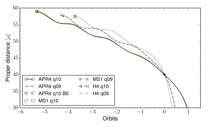
Figure 1: Proper separation between barycenters of the NSs versus orbital phase. The separation is plotted in units of reduced mass $\mu=M_{\mathrm{g}}^{1}M_{\mathrm{g}}^{2}/(M_{\mathrm{g}}^{1}+M_{\mathrm{g}}^{2})$, and the orbital phase is defined relative to a separation of $40\usk\mu$. Barycenter and orbital phase are computed with respect to simulation coordinates.

Table 2: Outcome of our BNS mergers. $M_{\mathrm{BH}}$ and $J_{\mathrm{BH}}$ are black hole mass and angular momentum $3.4\usk\mathrm{m}\mathrm{s}$ after formation (only for collapsing models). $M_{\mathrm{blk}}$ and $R_{\mathrm{blk}}$ are bulk mass and bulk radius (see text for definitions), while $\nu_{\mathrm{c}}$ and $\nu_{\mathrm{max}}$ denote the remnants central and maximum rotation rates, all computed $20\usk\mathrm{m}\mathrm{s}$ after merger. $f_{\mathrm{merge}}$ is the gravitational wave instantaneous frequency at the time of merger, $f_{\mathrm{pm}}$ is the frequency of the maximum in the post-merger part of the gravitational wave power spectrum, and $f_{10}$ is the average instantaneous frequency during the first $10\usk\mathrm{m}\mathrm{s}$ after merger (see Section VIII). $M_{\mathrm{disk}}$ is the mass outside the apparent horizon, or the mass outside $r>20$ km if no black hole is formed. $M_{\mathrm{fb}}$ is the bound mass outside $r>60$ km. Both are measured at $t=3.4\,\mathrm{ms}$ after black hole formation, or $t=20\,\mathrm{ms}$ after merger if no black hole is formed. Finally, $M_{\mathrm{ej}}$ and $v_{\mathrm{esc}}$ are our estimates for the total ejected mass and the average escape velocity. The values in brackets for the APR4 model refer to the high-resolution run (the measures absent for the standard resolution run were not implemented at the time).

Model	APR4 equal	APR4 unequal	MS1 equal	MS1 unequal	H4 equal	H4 unequal
$M_{\mathrm{BH}}\,[M_{\odot}]$	—	—	—	—	$2.49$	$2.42$
$J_{\mathrm{BH}}/M^{2}_{\mathrm{BH}}$	—	—	—	—	$0.63$	$0.57$
$M_{\mathrm{blk}}\,[M_{\odot}]$	($2.47$)	$2.42$	$2.35$	$2.25$	$2.48$	$2.37$
$M_{\mathrm{blk}}/R_{\mathrm{blk}}$	($0.30$)	$0.30$	$0.21$	$0.21$	$0.27$	$0.26$
$\nu_{\mathrm{c}}\,[\mathrm{kHz}]$	$0.73$ ($0.69$)	$0.64$	$0.34$	$0.27$	$0.69$	$0.52$
$\nu_{\mathrm{max}}\,[\mathrm{kHz}]$	$1.65$ ($1.64$)	$1.59$	$0.99$	$1.01$	$1.35$	$1.24$
$f_{\mathrm{merge}}\,[\mathrm{kHz}]$	$2.12$ ($2.12$)	$2.09$	$1.46$	$1.36$	$1.54$	$1.51$
$f_{\mathrm{pm}}\,[\mathrm{kHz}]$	$3.35$ ($3.33$)	$3.24$	$2.03$	$2.09$	$2.54$	$2.55$
$f_{10}\,[\mathrm{kHz}]$	$3.33$ ($3.32$)	$3.25$	$1.97$	$1.96$	$2.45$	$2.36$
$M_{\mathrm{disk}}\,[M_{\odot}]$	($0.201$)	$0.252$	$0.387$	$0.479$	$0.126$	$0.211$
$M_{\mathrm{fb}}\,[M_{\odot}]$	($0.121$)	$0.133$	$0.180$	$0.191$	$0.105$	$0.175$
$M_{\mathrm{ej}}\,[10^{-2}\,M_{\odot}]$	$1.31$ ($1.27$)	$0.74$	$0.08$	$0.09$	$0.07$	$0.10$
$v_{\mathrm{esc}}\,[c]$	($0.12$)	$0.10$	$0.10$	$0.10$	$0.11$	$0.13$

We note that half of the total magnetic energy corresponds to the value for a magnetized NS with a simple purely poloidal/dipolar configuration and $B_{\mathrm{pole}}\approx 2.4\times 10^{14}$ G (as computed with the “magstar” LORENE code). For more realistic configurations including also a strong toroidal magnetic field inside the NS, the same magnetic energy could even correspond to a $B_{\mathrm{pole}}$ as low as $\sim 10^{13}$ G Ciolfi and Rezzolla (2013). Since NSs in binary systems are expected to have $B_{\mathrm{pole}}\sim 10^{12}$ G, we are imposing magnetic energies a factor of $10^{2}-10^{4}$ higher than the common expectations. Nevertheless, GRMHD simulations of BNS mergers performed at very high resolution have recently confirmed that when magnetic field amplification mechanisms such as the Kelvin-Helmholtz instability are well resolved, the magnetic field can easily reach strengths of the order of $\sim 10^{15}$ G or higher (see Kiuchi et al. (2015) and refs. therein). Since our resolution is insufficient to fully resolve these amplification mechanisms, a lower (and more realistic) initial magnetic energy would result in a post-merger magnetic field orders of magnitude weaker than expected. For the resolution that we can currently afford, our choice allows us to explore more realistic post-merger field strengths despite the lower amplification factors. We stress, however, that this is by no means equivalent to fully resolving the amplification of a weaker initial field up to ${\sim}10^{15}$ G or more. We also note that the magnetic field strengths we impose are still sufficiently low to safely neglect deviations from hydrostatic equilibrium as well as constraint violations (magnetic energy is ${\sim}10^{6}$ times smaller than the binding energy of each NS).

For the evolution we use our GRMHD code Whisky Giacomazzo and Rezzolla (2007); Giacomazzo et al. (2011); Giacomazzo and Perna (2013) coupled with the publicly available Einstein Toolkit Löffler et al. (2012). The Einstein Toolkit is a collection of publicly available codes, including the Cactus computational framework, the Carpet driver, and the McLachlan code. In particular we use the McLachlan code to evolve Einstein’s equations using the BSSNOK formulation for the spacetime Baumgarte and Shapiro (1998); Shibata and Nakamura (1995); Nakamura et al. (1987). The GRMHD equations are instead evolved by our Whisky code, which uses high-resolution shock-capturing schemes to solve the GRMHD equations written in a flux-conservative form via the “Valencia” formulation Anton et al. (2006). The fluxes are computed with the HLLE approximate Riemann solver Harten et al. (1983) that uses the primitive variables reconstructed at the interfaces between the cells via the piecewise-parabolic method Colella and Woodward (1984). In order to preserve the divergence-free character of the magnetic field, we evolve the vector potential and compute the magnetic field from it. To avoid spurious magnetic field amplifications at the boundaries between refinement levels, we use the modified Lorenz gauge Etienne et al. (2012); Farris et al. (2012). We also set a density floor for the rest-mass density $\rho$ equal to $\rho_{\rm atmo}=10^{-11}\approx 6.2\times 10^{6}$ g cm^-3. Where $\rho$ falls below that value, we reset it to $\rho_{\rm atmo}$ and set the velocity to zero.

In all our simulations we use “moving box” mesh refinement provided by the Carpet driver. We use six refinement levels, with the grids of the two finest levels following each of the two NSs during the inspiral phase. At merger, we switch to fixed mesh refinement, with a central finest grid covering a radius of $30\usk\mathrm{k}\mathrm{m}$, large enough to contain the remnant object and the innermost part of the disk. We employ a resolution on the finest grid of $dx\approx 220$ m. This fiducial resolution allows us to cover the radii of the initial NSs with $\approx 50-70$ points, depending on the EOS. The equal-mass APR4 model is also evolved at higher and lower resolutions in order to assess the numerical accuracy (see the Appendix). The highest resolution employed in this work (for only one simulation) is $dx\approx 177$ m. We note that recent GRMHD simulations of BNS mergers have been also performed with higher or much higher resolution Kiuchi et al. (2014, 2015). The outer boundary of our computational domain is located at $\approx 1250$ km. To save computational resources we also enforce a reflection symmetry across the $z=0$ plane.

III Merger and postmerger dynamics

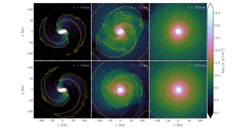
Figure 2: Rest mass density evolution on equatorial plane for the APR4 equal-mass (top row) and unequal-mass (bottom row) models. The contours indicate matter ejected that is unbound according to the geodesic criterion (see Section VII). The times of the snapshots denote the time after merger.

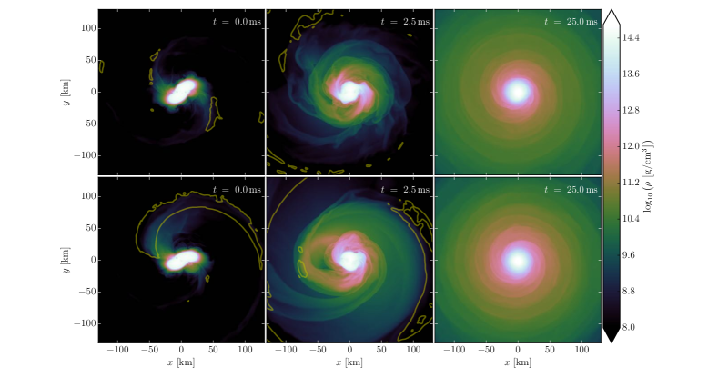
Figure 3: Same as Fig. 2 for MS1 equal-mass (top row) and unequal-mass (bottom row) models.

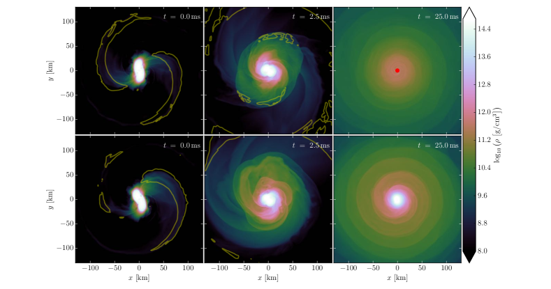
Figure 4: Same as Fig. 2 for H4 equal-mass (top row) and unequal-mass (bottom row) models. For the equal-mass model at $25\usk\mathrm{m}\mathrm{s}$ (upper right panel), a black hole is already formed, and the red disk indicates the apparent horizon.

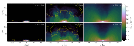
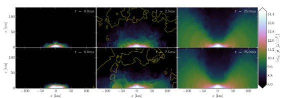
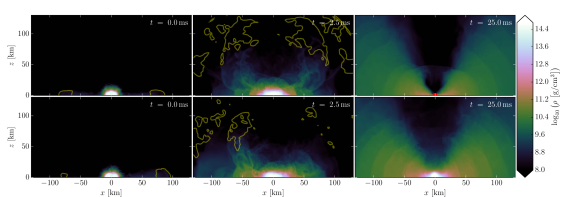
Figure 5: Same as Figures 2 to 4 but for the rest mass density on the meridional plane. From top to bottom: APR4, MS1, and H4 models.

In this Section, we describe basic aspects of the dynamics of the six reference models considered in this work. The key numeric results are listed in Table 2. We recall that four of these models form long-lived NSs (supramassive or stable for the APR4 and MS1 EOS, respectively), while the two models employing the H4 EOS produce a HMNS collapsing to a BH within few tens of ms.

The inspiral phase is shown in Fig. 1, depicting the separation versus orbital phase. We observe a clear trend for the impact of the EOS: the more compact the stars (see Table 1), the more orbits before merger. Note the oscillations around the overall decrease in separation correspond to the residual eccentricity of the initial data. Correcting the eccentricity might lead to some quantitative changes, but not enough to affect the general trend (see, e.g., Maione et al. (2016) and refs. therein for more details on eccentricity in BNS merger simulations).

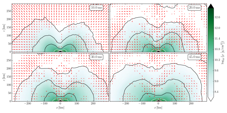
Figure 6: Velocity (arrows) and density (color and contour lines) in the meridional plane for the equal-mass APR4 model, at times $10,20,30,45\usk\mathrm{m}\mathrm{s}$ after merger, averaged over the time interval $\pm 2\usk\mathrm{m}\mathrm{s}$ to remove the contribution of oscillations. The contours correspond to $10^{-n}$ of the initial central density, with $n=1\ldots 6$. Note that the scale of the arrows is not the same in all panels, with the maximum velocities being $v/c=0.05\,(t=10\usk\mathrm{m}\mathrm{s}),\,0.09(20\usk\mathrm{m}\mathrm{s}),\,0.05(30\usk\mathrm{m}\mathrm{s}),\,0.07(45\usk\mathrm{m}\mathrm{s})$.

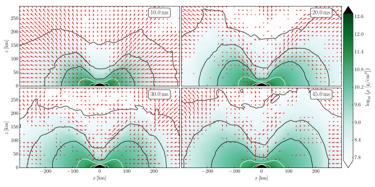
Figure 7: Like Fig. 6, but for the equal-mass MS1 model. Note that the scale of the arrows is not the same in all panels, with the maximum velocities being $v/c=0.08\,(t=10\usk\mathrm{m}\mathrm{s}),0.05\,(20\usk\mathrm{m}\mathrm{s}),0.05\,(30\usk\mathrm{m}\mathrm{s}),\,0.06(45\usk\mathrm{m}\mathrm{s})$.

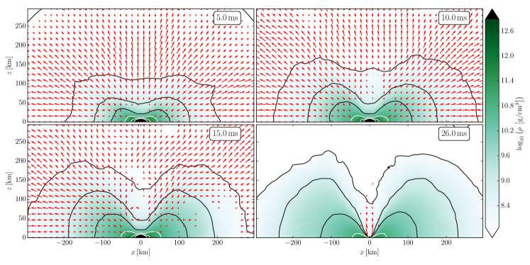
Figure 8: Like Fig. 6, but for the equal-mass H4 model. Note that the scale of the arrows is not the same in all panels, with the maximum velocities being $v/c=0.13\,(t=5\usk\mathrm{m}\mathrm{s}),0.07\,(10\usk\mathrm{m}\mathrm{s}),0.05\,(15\usk\mathrm{m}\mathrm{s}),0.40\,(26\usk\mathrm{m}\mathrm{s})$. The black disk in the lower right panel marks the apparent horizon.

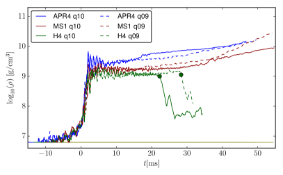
Figure 9: Evolution of rest-mass density along the $z$ axis, averaged between $z=30\usk\mathrm{k}\mathrm{m}$ and $z=50\usk\mathrm{k}\mathrm{m}$. The horizontal line marks the density of the artificial atmosphere.

Differences between mass ratios $1$ and $0.9$ are instead very small. Comparing the equal-mass APR4 model to the corresponding unmagnetized case, we also find that the magnetic field of the given strength has no impact on the inspiral phase.

An overview of the merger and post-merger evolution is given in Figures 2 to 4, showing snapshots of the rest-mass density in the orbital plane at times $0,2.5,25\usk\mathrm{m}\mathrm{s}$ after merger. We define the time of merger, $t_{\mathrm{merge}}$, as the retarded time at which the GW signal reaches its maximum amplitude. Throughout this article, all times are given relative to $t_{\mathrm{merge}}$, i.e. times generally refer to the time after merger. Fig. 5 shows the same evolution as seen on the meridional plane. From those figures it is clear that, after a highly dynamic merger phase, the system settles within $\sim\!20\usk\mathrm{m}\mathrm{s}$ to a quasi-stationary state composed of a massive NS surrounded by an accretion disk. For the APR4 and MS1 models, such a configuration remains almost unchanged until the end of the simulations (more than $45\usk\mathrm{m}\mathrm{s}$ after merger), while for the H4 models a BH is formed respectively $22$ and $28\usk\mathrm{m}\mathrm{s}$ after merger for the equal and unequal-mass cases.

In order to quantify the disk mass, we provide in Table 2 the total mass either outside the apparent horizon or outside a radius $r>20\usk\mathrm{k}\mathrm{m}$ if no BH is formed. In the equal-mass case, this estimate gives $M_{\mathrm{disk}}\!\approx\!0.2\,M_{\odot}$ for APR4 and almost $0.4\,M_{\odot}$ for MS1. Going from equal to unequal mass, both models result in a $\sim\!25\%$ higher disk mass. For the H4 models, a few ms after collapse the BH is surrounded by a disk of $\sim\!0.13\,$($0.21$) $M_{\odot}$ for equal (unequal) mass. In this case, the mass ratio has a much larger impact on $M_{\mathrm{disk}}$. We note that the HMNS lifetime is also longer for the unequal-mass case. Part of the increased disk mass could be due to a higher amount of matter expelled from the remnant via oscillations or shocks. The properties of the BHs shortly after formation are very similar for equal- and unequal-mass case, with BH masses of $2.50\,M_{\odot}$ and $2.42\,M_{\odot}$, and spins of $0.62$ and $0.57$, respectively. Since the disk smoothly transitions into a fallback component on non-circular orbits, we also provide the mass outside $r>60\usk\mathrm{k}\mathrm{m}$, $M_{\mathrm{fb}}$, as a ballpark figure for the outer disk/fallback component. We find that $40$–$80\%$ of the total disk mass is outside $60\usk\mathrm{k}\mathrm{m}$.

Figures 2 to 5 also show regions of matter that is unbound according to the geodesic criterion. In all models, we can distinguish a tidal contribution to the ejected matter confined to the equatorial plane (clearly visible at $t\!=\!0$) and a later, more isotropic ejection which we attribute to breakout shocks. Our best estimate for the amount of unbound matter is given in Table 2. A more detailed discussion on mass ejection is given in Sec. VII.

For the long-lived remnant cases (APR4 and MS1 models), the above dynamical ejecta are followed by a slower outflow of material that is bound according to the geodesic criterion, and that might fall back onto the remnant at later times. As will be discussed in Sec. VII, it is also possible that some of this matter will become unbound as a result of the magnetic pressure, and constitute a baryon-loaded wind. Note that such winds are likely to play an important role for the long-term EM emission from the supramassive or stable NS (e.g. Yu et al. (2013); Metzger et al. (2014); Ciolfi and Siegel (2015a); Siegel and Ciolfi (2016a, b)). Density and velocity of the outflow in the meridional plane are shown at different times in Figures 6 and 7. Since we are not interested in fluctuations, we averaged over a duration of $4\usk\mathrm{m}\mathrm{s}$. We find a relatively isotropic radial outflow with maximum velocities around $0.05$–$0.08\usk c$ at $t=10\usk\mathrm{m}\mathrm{s}$. At $t>20\usk\mathrm{m}\mathrm{s}$ however, the flow patterns consist mainly of large eddies, with a smaller net flux. These post-merger matter outflows will be discussed further in Sec. VII.

For the H4 models, we find a strong influx of matter along the $z$ axis after the BH is formed, as shown in Fig. 8. This is expected since matter along the $z$ axis could only be supported by the vertical pressure gradient, which can only be sustained by a NS remnant, not a BH. The inflow after the collapse quickly leads to a funnel of reduced density.

The baryon pollution along the orbital axis has important consequences for the possibility of launching relativistic jets which could give rise to SGRBs Murguia-Berthier et al. (2014); Nagakura et al. (2014); Murguia-Berthier et al. (2016) (see Section VI). Fig. 9 shows the density averaged along the $z$ axis between $z=30$ and $z=50\usk\mathrm{k}\mathrm{m}$. For all models, we find densities of the order $10^{9}\usk\mathrm{g}\mathrm{/}\mathrm{c}\mathrm{m}\mathrm{{}^{3}}$ few ms after merger, and subsequently a slow and persistent increase. For the H4 models, the density drops sharply by almost two orders of magnitude when a BH is formed. At least for the equal-mass model, the density seems to stabilize at this level or even increase slightly. The unequal-mass simulation ends shortly after BH formation, but we expect a similar behavior.

IV Rotation profile and remnant structure

In the following, we investigate the structure of the fluid flow inside the remnant in the equatorial plane, focusing at first on the H4 models. As in Kastaun et al. (2016a); Kastaun and Galeazzi (2015), we track fluid elements in a frame corotating with the $m=2$ component of the density deformation. The fluid flow together with the density distribution at different times are shown in Fig. 10 for the H4 equal-mass case and in Fig. 11 for the H4 unequal-mass case. As one can see, the remnants are still strongly deformed at $15\usk\mathrm{m}\mathrm{s}$ after merger. We also find that the fluid flow does not correspond to simple differential rotation. Instead, we observe secondary vortices. Those vortices are related to the density deformation, although it is unclear if they are causing it or are caused by it. Most likely, both density deformation and vortices influence each other. In any case, the vortices remain stationary with respect to the deformation most of the time, although there is some gradual evolution towards a more axisymmetric state. For the unequal-mass model however, a more rapid rearrangement seems to happen between $5$–$11\usk\mathrm{m}\mathrm{s}$ after merger. Also, not surprisingly, the structure shortly after merger is decidedly less symmetric for the unequal-mass case. We note that a similar rearrangement of vortices and deformation pattern has been found in Kastaun and Galeazzi (2015) for a binary model with equal mass, but unequal NS spin. It is also worth pointing out that, roughly speaking, the deformation of the outer layers is rotated 90 degrees with respect to the core, which implies contributions to the quadrupole moment with opposite signs. The impact on the GW signal will be discussed further in Sec. VIII.

For the long-lived remnant cases (APR4 and MS1), similar structures appear in the early post-merger phase. Nevertheless, within $15-20$ ms the system settles to a more ordered quasi-stationary structure characterized by simple differential rotation (see, e.g., Fig. 9 of Kastaun et al. (2016b), showing the same as Fig. 10 for our unmagnetized APR4 equal-mass model).

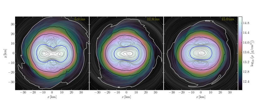
Figure 10: Remnant structure in the equatorial plane at different times for the equal mass H4 model. The density is shown as color plot. The thick lines are isodensity contours at $0.5$, $0.1$, $0.01$, $0.001$ times the maximum density. The thin lines are fluid trajectories in a frame corotating with the $m=2$ density deformation, during a time interval $\pm 1\usk\mathrm{m}\mathrm{s}$ around the time of each snapshot.

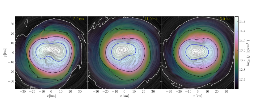
Figure 11: Like Fig. 10, but showing the unequal-mass H4 model.

We now turn to discuss the rotation profiles of the remnants. For this, we employ the methods described in Kastaun and Galeazzi (2015). In particular, we use a coordinate system that is defined independent of the spatial gauge conditions and prevents non-axisymetric as well as spiral distortions, given that the spacetime is axisymmetric (see Kastaun and Galeazzi (2015) for details). We restrict the analysis to the equatorial plane, because the new coordinate system is only defined there and the required data is saved only on coordinate planes.

Fig. 12 shows the rotation rate for all models at a time $20\usk\mathrm{m}\mathrm{s}$ after merger. To reduce the influence of residual oscillations, we average over the time interval $20\pm 1\usk\mathrm{m}\mathrm{s}$. All the rotation profiles show a clear maximum away from the center, and a slow central rotation rate below $0.8\usk\mathrm{k}\mathrm{Hz}$. Fig. 12 also shows part of the disk, which smoothly joins the remnant. For $r>20\usk\mathrm{k}\mathrm{m}$, the rotation rates are given approximately by the Kepler velocity, which depends almost exclusively on the remnant mass. Our findings are similar to the results obtained for different models in Kastaun and Galeazzi (2015); Endrizzi et al. (2016); Kastaun et al. (2016a, b); Hanauske et al. (2016). The models in those publications together with the present one include hypermassive, supramassive, and stable remnants, different mass ratios, and even binaries with initial aligned spin. The general shape of the rotation profiles shown in Fig. 12 seem to be a generic property of merger remnants.

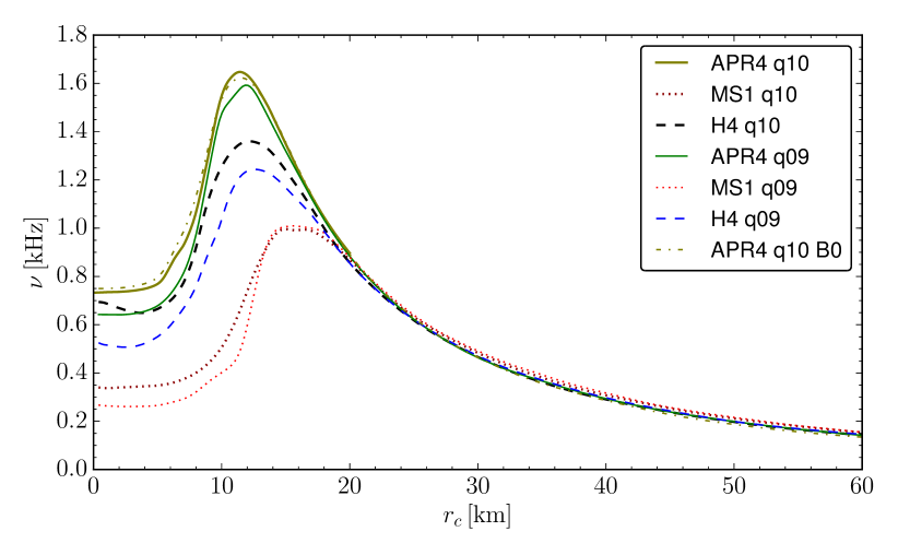
Figure 12: Rotation rate (as seen from infinity) in the equatorial plane $20\usk\mathrm{m}\mathrm{s}$ after merger, averaged in $\phi$ and over a time window of $\pm 1\usk\mathrm{m}\mathrm{s}$, versus circumferential radius.

Since the rotation profiles show that the cores are rotating slowly, we expect that the inner core can be approximated by a spherical TOV solution. In order to judge the importance of centrifugal forces in the core, we computed the ratio of rotation rate and orbital frequency of a test mass in circular orbit (both measured by zero angular momentum observers, i.e. removing the frame dragging) at the center of the remnants $20\usk\mathrm{m}\mathrm{s}$ after merger. We found values ranging between $0.02$ (APR4 unequal-mass model) and $0.06$ (H4 equal-mass model). This indeed strongly suggests TOV-like cores. In order to quantify the radial mass distribution in an unambiguous way, we use the measures described in Kastaun et al. (2016a). These replace the density versus radius measures used for spherical stars with the baryonic mass as function of proper volume contained in isosurfaces of constant rest mass density. Further, to express compactness of the remnant in absence of a clear surface, we define the compactness of each isodensity surface as the ratio between the contained baryonic mass and the radius of an Euclidean sphere with the same proper volume. This compactness has a maximum, which we use to define the bulk isodensity surface, and the corresponding bulk compactness, bulk mass, and bulk volume.

The mass-versus-volume relations for the merger remnants are shown in Fig. 13, while the bulk properties of the remnants are given in Table 2. For the models at hand, the radial mass distribution and the bulk compactness are mainly determined by the EOS, while the mass ratio has a minor impact (at fixed total gravitational mass). Fig. 13 also shows the relation of bulk mass versus bulk volume for sequences of TOV solutions with the EOS used in this work. We use the intersection with the remnant profile to find a TOV model approximating the inner core of the remnant, called TOV core equivalent in the following. By comparing the mass-versus-volume relation of the TOV core equivalent and the remnant, we find that the structure of the core of the remnants is very well approximated by TOV core equivalent solutions. Fig. 13 also shows that the differences between TOV equivalent and actual remnant become gradually larger between the bulk of the TOV core equivalent (square symbol) and its surface. This is due to the fact that for the remnant, centrifugal forces become important in the outer envelope.

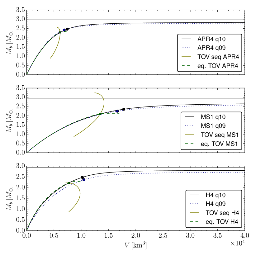
Figure 13: Mass versus volume relations of the merger remnant isodensity surfaces, $20\usk\mathrm{m}\mathrm{s}$ after merger. The maximum compactness shell (the bulk) is marked by circle symbols. For comparison, we show bulk mass and bulk volume (see text) of TOV sequences obtained with the same EOS (continuous yellow line), and the mass-volume relation of the TOV core equivalent approximating the inner remnant core (dashed green line, bulk marked by square symbol). Horizontal grey lines mark the total baryon mass of the system.

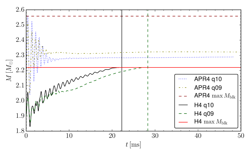
Figure 14: Evolution of the bulk mass of the TOV core equivalent approximating the merger remnant for the H4 and APR4 models. The horizontal lines mark the maximum bulk mass of stable TOV solutions for each EOS, while the vertical lines mark black hole formation.

It is reasonable to assume that if there is no stable TOV solution approximating the inner core, it either has to rotate more rapidly or collapse. This gives us another critical mass, namely the bulk mass of the maximum (gravitational) mass TOV star. This mass is $2.56\usk M_{\odot}$ for the APR4 EOS, $2.22\usk M_{\odot}$ for the H4 EOS, and $3.24\usk M_{\odot}$ for the MS1 EOS. Note that for the H4 simulations, the bulk mass of the TOV core equivalent is very close to the maximum value allowed for a stable star, while for the other models it is much lower. At the same time, only the H4 models collapsed to a BH on the timescale of the evolution. To investigate this aspect further, we computed the evolution of the TOV core equivalent bulk mass for the H4 models, which is shown in Fig. 14. For those two runs, the core mass slowly approaches the critical one, and the collapse occurs as soon as the latter is reached. We therefore propose a new conjecture: merger remnants that do not admit a TOV core equivalent promptly collapse to a BH. This differs from the classification into supra- and hypermassive stars because it is a constraint on the mass of the inner core, not the total mass. An important consequence is that, given the EOS, the presence of a post-merger phase (e.g., observed via the post-merger GW signal) would put a constraint on the mass, volume, and compactness of the inner core.

Of course, our conjecture needs to be validated for more models. Also, it is meant for the phase when the remnant has settled down and can be regarded as stationary, not for the strongly oscillating phase directly after merger. If it is also relevant for this phase is however an interesting question. For example, Fig. 14 also shows the APR4 models, for which the core equivalent of the late remnant is well below the critical mass. During the early post-merger phase, however, it comes very close to the critical value for a short time. According to Hotokezaka et al. (2011), the threshold for prompt collapse of equal mass binaries with the APR4 EOS is reached at a single star ADM mass around $1.4\usk M_{\odot}$. Our APR4 equal-mass model with $M_{g}=1.35\usk M_{\odot}$ is indeed close to this threshold.

Another noteworthy observation is that the TOV core equivalents of the equal- and unequal-mass H4 models are very similar for the first $6\usk\mathrm{m}\mathrm{s}$ after merger and then suddenly start to differ. This might be caused by the aforementioned change in the fluid flow happening around the same time. If the two events are in fact related, it would imply that the vortex structure also has a direct impact on HMNS lifetimes.

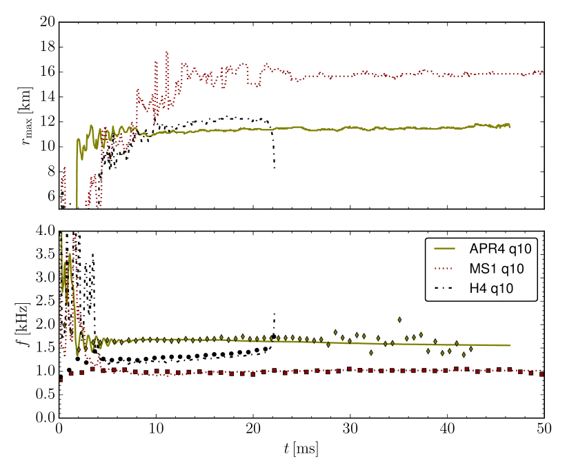
Figure 15: Top panel: location of the maximum of the rotation profile shown in Fig. 12 as function of time. Bottom panel: maximum rotation frequency (lines) compared to half of the gravitational wave instantaneous frequency (markers).

Returning to the rotation rate of our models shown in Fig. 12, we find that (for the given total mass) the EOS has a much stronger influence on the maximum rotation rate than the mass ratio. The APR4 EOS results in the highest rotation rate, followed by the H4 EOS, and then the MS1 EOS. We also notice a correlation between the maximum rotation rate and the position of the maximum, which is located further out for the models with smaller maximum rotation rate. Intuitively, one might expect more compact models to rotate faster. We find indeed that the bulk compactness of the remnants follows the same ordering as the maximum rotation rate, with the most compact remnant obtained for the APR4 case (see Table 2). For the equal-mass APR4 model, Fig. 12 also shows the profile for the non-magnetized case, which is almost identical to the magnetized one.

The time evolution and radial location of the maximum rotation rate are shown in Fig. 15. Directly after merger, the maximum is located near the origin, although this measure is not meaningful during this phase because the fluid flow cannot be described as simple differential rotation. After around $5\usk\mathrm{m}\mathrm{s}$, however, the remnant has settled down to a state similar to Fig. 12, with the maximum at the outer layers. Subsequently, the APR4 and MS1 models show only minor drifts of the maximum rotation rate on the timescale of the simulation. Also the location of the maximum varies only slightly. This indicates that the remnant will change on timescales much longer than the time window covered by our simulation. The H4 model on the other hand exhibits a moderate increase of the rotation rate until the collapse to a BH occurs. Fig. 15 also shows the instantaneous GW frequency. The GW signal will be discussed in detail in Sec. VIII. Here we point out that the angular velocity of the $m=2$ GW pattern (i.e. half the GW frequency) closely follows the maximum rotation rate. This is not surprising if the maximum rotation rate is tied to the main $m=2$ deformation of the remnant, which seems to be the case. This relation seems robust, as it was also found for different models in Kastaun and Galeazzi (2015); Endrizzi et al. (2016); Kastaun et al. (2016a); Hanauske et al. (2016) and we are not aware of a single counter-example.

V Magnetic fields

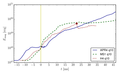
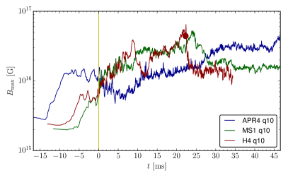
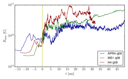
Figure 16: Evolution of magnetic energy (left) and maximum magnetic field strength (right) for the equal-mass (top) and unequal-mass (bottom) models. The vertical line marks the time of merger. The red circle (H4 EOS) marks the time of collapse to black hole.

In this Section we discuss the evolution of magnetic fields. Fig. 16 (left panels) shows the magnetic energy evolution for the different EOS and mass ratios considered in this work. All of our BNS models experience magnetic field amplification prior to merger, starting when the two NSs are at a proper distance of $\sim\!54$ km. After a few ms and about one order of magnitude increase in magnetic energy, the amplification can stall for some time and continue when the two NS cores effectively merge. Depending on the EOS, this stalling can last up to $\sim\!10$ ms (APR4 case) or be absent (MS1 case), with a duration that increases with compactness. This might simply be due to the different duration of the inspiral phase.

The cause of the pre-merger amplification and its saturation is still unclear. As discussed in the Appendix, the initial growth does not seem to be a result of insufficient resolution, although we cannot rule out that it is caused by interaction of the NSs with the artificial atmosphere. The violations of the GR constraint equations introduced by adding the magnetic field can safely be neglected, and also the deviation from hydrostatic equilibrium due to the additional magnetic pressure is too small and will only lead to small oscillations. By looking at the magnetic field strength at the boundaries of the moving grids during inspiral, we find no evidence of spurious magnetic field amplification. However, we cannot exclude that generic imperfections of the initial data lead to fluid flows that amplify the magnetic field. For the saturation phase, the resolution has a larger influence and it is not clear if the saturation is a purely numerical artifact or if the saturation mechanism is physical, but harder to resolve. Another effect that can be excluded is the development of a hydromagnetic instability such as the Tayler instability of purely poloidal magnetic fields Markey and Tayler (1973), since the Alfvén timescale inside the NSs before merger is at least one order of magnitude larger than the observed amplification timescale (see e.g. Ciolfi et al. (2011)).

The only remaining physical explanation seems to be the time-changing tidal deformation during the inspiral. Although it is by no means clear how it would amplify the field, we note that a recent study Dall’Osso and Rossi (2013) suggested that the tidal forces can drive significant fluid flows inside the NSs in the late inspiral. If the observed amplification was indeed a physical effect, it would be very interesting. In particular, we note that all models end up with the same magnetic energy at the time of merger, independent of mass ratio and EOS. This would indicate that the magnetic energy at merger might be determined by the saturation scale of the mechanism responsible for the amplification. We stress again that our findings are not conclusive since we cannot rule out unphysical causes. In any case, the topic deserves further investigation.

We also note that magnetic field amplification prior to merger was already reported in other studies. For instance, Kiuchi et al. Kiuchi et al. (2014) evolved an equal-mass H4 model with different initial magnetic field strengths and resolutions and obtained in all runs a factor $\sim 2$ amplification in magnetic energy in the last $5$ ms of pre-merger evolution (see Fig. 2 of Kiuchi et al. (2014)). Within the same $5$ ms time window, the above behavior is very similar to what we obtain for our equal-mass H4 model (see top left panel of Fig. 16).

When the two NSs merge, magnetic fields are strongly amplified by about one order of magnitude or more (factor $\sim 50-500$ in magnetic energy). One key mechanism that is known to strongly amplify the toroidal component of the field is the Kelvin-Helmholtz (KH) instability, which develops in the shear layer separating the two NS cores when they come into contact. This effect is most likely responsible for the particularly steep increase of magnetic energy during the first $5\usk\mathrm{m}\mathrm{s}$ observed in all our simulations. For unknown reasons, the onset of the amplification is slightly delayed for the APR4 models (respectively by ${\sim}4$ and ${\sim}1\usk\mathrm{m}\mathrm{s}$ for the equal- and unequal-mass cases). Judging by the initial growth of the magnetic energy, both EOS and mass ratio have an influence on the KH instability. The effect of the KH instability in the early post-merger phase is also evident in terms of maximum magnetic field strength Fig. 16 (right panels). After merger, this maximum is achieved in the equatorial region and corresponds to a magnetic field that is essentially toroidal. As a note of caution, we stress that the resolution employed in our simulations determines the smallest scale at which the KH instability is effective. As will be shown in the Appendix, the magnetic field after merger is not converging and higher resolution results in a steeper growth . Nevertheless, with higher resolution the magnetic fields experience a faster amplification but also an earlier saturation, and the magnetic energy achieved in the end does not differ by more than a factor of two (when comparing medium and high resolutions).

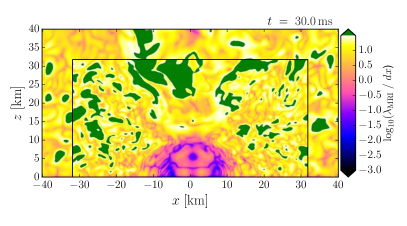
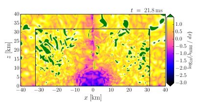
Figure 17: Meridional view of $\lambda_{\mathrm{MRI}}/dx$. This quantity gives an estimate of the number of grid points to resolve the wavelength of the fastest growing MRI mode (see text). Top: APR4 equal-mass case 30 ms after merger. Bottom: H4 equal-mass case, 0.5 ms prior to collapse.

For all models, the rapid growth attributed to the KH instability only lasts for a few ms, after which the magnetic energy can still grow by more than one order of magnitude. At this later stage, we assume that the KH instability is gradually substituted by other amplification mechanisms, associated with turbulence and/or differential rotation. Apart from magnetic winding, which is well resolved and contributes in part to the growth of the toroidal field, the amplification mechanisms at play are limited by the smallest scales we can resolve. A potentially powerful mechanism is the magnetorotational instability (MRI) Balbus and Hawley (1991); Duez et al. (2006b); Siegel et al. (2013). In order to assess whether the MRI is contributing to the observed amplification we estimated the wavelength of the fastest growing MRI mode as $\lambda_{\mathrm{MRI}}\approx(2\pi/\Omega)\times B/\sqrt{4\pi\rho}$, where $\Omega$ is the angular velocity and $B$ is the magnetic field strength . Typically, the MRI is effective in numerical simulations when $\lambda_{\mathrm{MRI}}$ is resolved with at least 10 grid points (see, e.g., Siegel et al. (2013)). As shown in Fig. 17, this requirement is satisfied in most of the region outside the remnant, for both long-lived (APR4 and MS1) and short-lived (H4) remnants. We conclude that MRI is likely playing an active role in our simulations.

Fig. 18 shows the magnetic field strength in the meridional plane 30 ms after merger. For all six models, the maximum field strength is in excess of $10^{16}$ G (cf. right panels of Fig. 16) and is achieved in the inner equatorial region. After this time, the hydrodynamic evolution of both the APR4 and MS1 models has reached a quasi-stationary state, while the magnetic energy keeps growing more or less exponentially. For APR4 models, the unequal-mass case shows a lower amplification rate at this later stage, while for MS1 models it is the other way around. This suggests that the magnetic field evolution depends on EOS and mass ratio in a complex way and that the effect of the two cannot be easily disentangled.

The overall amplification of magnetic energy $45\usk\mathrm{m}\mathrm{s}$ after merger is between two and three orders of magnitude with respect to the energy at merger time. Note that the initial amplification attributed to the KH mechanism only accounts for a small fraction of the final energy, and hence the final amplification factor is dominated by the late amplification via MRI and magnetic winding. From Fig. 17, we expect to resolve the MRI, at least outside the remnant. Our resolution study (see Appendix for details) indeed indicates that the final magnetic energy is starting to converge, in contrast to the early growth. We expect the final total magnetic energy to be accurate within an order of magnitude. With the MRI in the disk dominating the final magnetic energy, we would also not expect substantial changes when using a subgrid model Giacomazzo et al. (2015). Note that the numerical accuracy of the amplification strongly depends on the initial field strength, because the scale of the fastest growing MRI mode is proportional to the magnetic field. In a previous study Endrizzi et al. (2016) employing similar resolutions, we started with a much lower initial magnetic energy and found no indication for numerical convergence in the final value of $E_{\mathrm{mag}}$ (which was still smaller than the ones reached in this work). When taking our simulations as indication for real mergers with similar initial magnetic energy, we believe that the main uncertainty is not the numerical accuracy but the geometry of the initial magnetic field, in particular the field outside the stars. This aspect will be further investigated in future studies.

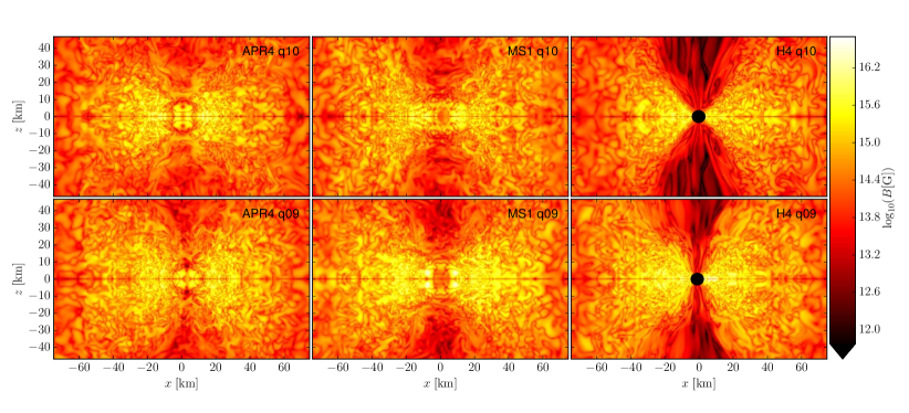
Figure 18: Meridional view of the magnetic field strength 30 ms after merger for different EOS (left to right: APR4, MS1, H4) and mass ratios (top row $q=1$, bottom row $q=0.9$). The region inside the apparent horizon is indicated in black (H4 case).

We now turn our attention to the geometrical structure of the magnetic field obtained towards the end of the simulations. For a qualitative description, we visualize the field lines using the same method as in Kawamura et al. (2016). In short, the method tries to show only the field lines with the largest average ratio of magnetic field strength to the maximum field strength at same $\theta$ coordinate. This is adapted to more or less axisymmetric configurations where the field strength varies strongly between the pole and the equatorial plane. For details, see Kawamura et al. (2016). Fig. 19 shows the field lines in 3D for the equal-mass MS1 and APR4 models $45\usk\mathrm{m}\mathrm{s}$ after merger. As already pointed out, the field is largest on the equatorial plane, where it is predominantly toroidal. The field around the axis is weaker and mostly unordered, with a slight tendency to helical structures. This is in contrast to the cases described in Kawamura et al. (2016), where the central object was a BH and where more ordered twister-like structures were found along a cone around the orbital axis. We expect that our H4 models, if evolved for long enough after collapse to a BH, would also develop a similar geometry. In the case of a long-lived remnant (APR4 and MS1 models), however, the formation of analogous structures on longer timescales cannot be excluded. A notable difference is that magnetic fields along the orbital axis, although disordered, can exceed $10^{14}$ G while in the cases where a BH is formed (H4 models) they hardly exceed $10^{13}$ G.

For a quantitative description of the field distribution in the polar angle $\theta$, we use the same measures as in Kawamura et al. (2016): we sum up the magnetic energy in a 2D histogram binned by $\cos(\theta)$ and magnetic field strength. For each bin in $\theta$, we define the field strength $B_{90}$ such that $90\%$ of the magnetic energy in the same bin is contained in regions with lower field strength. This measure is in-between average and maximum norm, but less sensitive to single points than the latter. We also compute the total energy in each $\cos(\theta)$ bin (regardless of field strength). The result is shown in Fig. 20. We find that for all models most of the magnetic energy is in the equatorial region. The characteristic field strength $B_{90}$, on the other hand, shows a different behavior for different models. The APR4 equal-mass case has a rather flat value around $10^{16}$ G between $\theta{\approx}40\mathrm{\SIUnitSymbolDegree}$ and $140\mathrm{\SIUnitSymbolDegree}$ (equatorial region) and around $3\times 10^{15}$ G near the axis. The APR4 unequal-mass has similar values except along a cone of half-opening angle of ${\approx}60\mathrm{\SIUnitSymbolDegree}$–$70\mathrm{\SIUnitSymbolDegree}$ around the spin axis, where $B_{90}$ is as strong as $4\times 10^{16}$ G. The MS1 equal-mass model has the lowest $B_{90}$ of ${\approx}10^{15}$ G along the axis and almost $10^{16}$ G in the equatorial region ($70\mathrm{\SIUnitSymbolDegree}$–$110\mathrm{\SIUnitSymbolDegree}$). Finally, the MS1 unequal-mass model has a rather flat value of $B_{90}{\approx}10^{16}$ G at all angles. These results show that there is no unique behavior at this stage of the evolution. In order to assess whether a common ordered structure would emerge at a later time (e.g., a structure favorable for jet formation), long-term simulations extending far beyond the timescales covered in this work are needed.

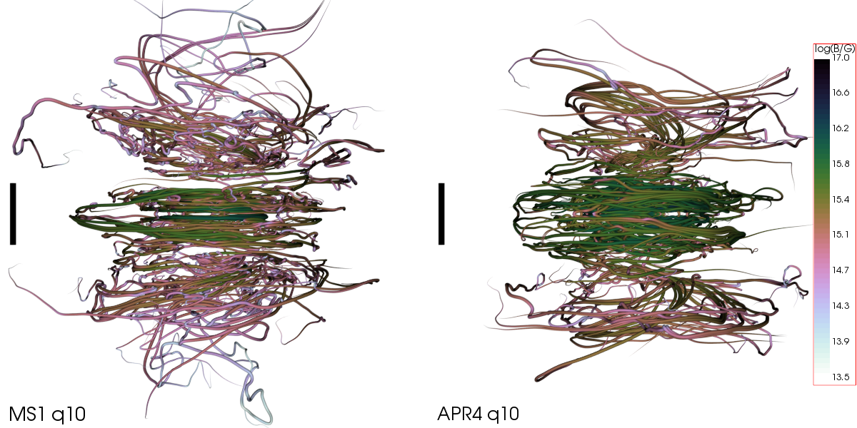
Figure 19: Structure of magnetic field $45\usk\mathrm{m}\mathrm{s}$ after merger for the equal-mass MS1 (left) and APR4 (right) models. The coloring indicates the magnetic field strength ($\log_{10}(B[\mathrm{G}])$, same color scale for both models). For more quantitative results see Fig. 20. The black bars provide a length scale of $20\usk\mathrm{k}\mathrm{m}$.

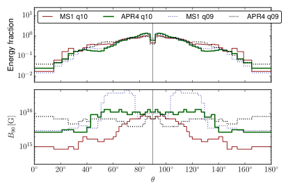
Figure 20: Distribution of magnetic field with respect to $\theta$-coordinate, for APR4 and MS1 models $45\usk\mathrm{m}\mathrm{s}$ after merger. Top: histogram of magnetic energy employing bins regularly spaced in $\cos(\theta)$, where $\theta=0$ on the positive $z$-axis and $\theta=90\mathrm{\SIUnitSymbolDegree}$ at the equator. Each curve is normalized to the total magnetic energy. Bottom: characteristic field strength $B_{90}$ defined as the value for which $90\%$ of the magnetic energy inside a given $\cos(\theta)$ bin is contributed by regions with field strengths below $B_{90}$.

VI Short gamma-ray bursts

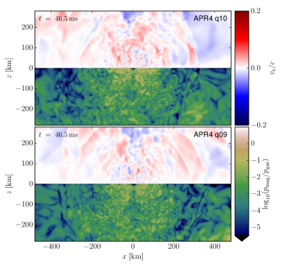
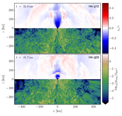
Figure 21: Meridional view of the fluid velocity perpendicular to the orbital plane (i.e. the $z$-component) and of the magnetic-to-fluid pressure ratio (on the top and bottom half of each panel, respectively), towards the end of our simulations. Left: APR4 models with equal mass (top) and unequal mass (bottom). Right: the same for H4 models (region in black is inside the apparent horizon).

In what follows, we discuss the results of our simulations in the context of SGRBs. BNS and NS-BH mergers represent primary candidates as progenitors of these events Paczynski (1986); Eichler et al. (1989); Narayan et al. (1992); Barthelmy et al. (2005); Fox et al. (2005); Gehrels et al. (2005); Shibata et al. (2006); Tanvir et al. (2013); Berger et al. (2013); Paschalidis et al. (2015); Ruiz et al. (2016). One main reason is that a common product of such mergers is a compact object (a massive NS or a BH) surrounded by an accretion disk of mass $\gtrsim\!0.1M_{\odot}$, and the corresponding accretion timescale ($\sim\!1$ s) matches the duration of the SGRB prompt emission ($<\!2$ s). In addition, the lack of supernova associations, the diverse types of host galaxies (which include also early-type galaxies), and the large offsets from the center of the host galaxy, are all in favor of a binary compact object origin Berger (2014).

The most commonly discussed scenario is the one in which a compact binary merger leads to the prompt formation of a BH surrounded by a massive accretion disk . The accretion onto the BH is what provides the source of power. Since the gamma-ray emission is believed to be generated within a relativistic outflow, an additional key ingredient is the ability of the system to drive a jet. Two main mechanisms have been proposed as energy sources capable of launching a jet: (i) the deposition of thermal energy at the poles of the BH via the annihilation of neutrinos and antineutrinos copiously emitted by the hot accretion disk Eichler et al. (1989); Ruffert and Janka (1999), and (ii) the action of large scale magnetic fields threading the accretion disk and tapping the rotational energy of the BH via the Blandford-Znajek mechanism Blandford and Znajek (1977) (analogous to the well established case of AGNs/blazars McKinney and Blandford (2009)). Recent simulations indicate that the neutrino mechanism, while potentially important, seems to be too weak to drive a powerful enough jet on its own, especially in the BNS merger case Just et al. (2016); Perego et al. (2017). Hence, the energy requirements favor magnetic fields as the main driving force.

In the last few years, GRMHD simulations of BNS or NS-BH mergers provided important hints on the possibility of launching a magnetically driven jet (e.g. Rezzolla et al. (2011); Kiuchi et al. (2014); Paschalidis et al. (2015); Ruiz et al. (2016); Kawamura et al. (2016)). In particular, Ruiz et al. Ruiz et al. (2016) reported for the first time in a BNS merger simulation the emergence of a collimated and mildly relativistic outflow along a baryon-poor and magnetically dominated funnel surrounding the BH spin axis (referred to as “incipient jet”). A similar result was obtained earlier for the NS-BH case Paschalidis et al. (2015). No other group has so far reported an analogous result. In the most recent paper on the subject Kawamura et al. (2016), BNS merger simulations performed by our group showed the formation of a twister-like magnetic field structure along the spin axis of the BH, but no net outflow was found, nor a magnetically dominated funnel.

Our present simulations forming a BH-disk system (models with the H4 EOS) are too short to assess if the post-collapse system would evolve in a similar way and possibly form an incipient jet at later times. As shown in Fig. 21 (right panels), a few ms after collapse matter is still largely infalling along the BH spin axis. Magnetic pressure is becoming comparable to the gas pressure at the edges of the disk, but it is still generally subdominant inside the baryon-poor funnel.

The main focus of this work, however, is on magnetized BNS mergers forming a long-lived NS. The possibility that such a remnant could act as the central engine of a SGRB was put forward by the so-called magnetar model Zhang and Mészáros (2001); Gao and Fan (2006); Metzger et al. (2008), which represents the most popular alternative to the standard BH-disk scenario. In this case, an accretion-powered jet is launched by a strongly magnetized NS surrounded by a massive accretion disk. While this is viable for BNS mergers, it clearly excludes NS-BH binaries as the possible progenitor. The magnetar model was recently revived, after the observation by the Swift satellite Gehrels et al. (2004) of long-lasting ($\sim$minutes to hours) X-ray afterglows accompanying a significant fraction of all SGRB events Rowlinson et al. (2013); Lü et al. (2015). This evidence poses a challenge to the BH-disk scenario, as the short accretion timescale onto the BH can hardly be reconciled with a sustained emission lasting $\gtrsim\!100-1000$ s. Within the magnetar model, thanks to the EM spindown emission from the magnetized NS, these afterglows might find instead a natural explanation. Moreover, the observation of NSs with a mass of $\approx\!2M_{\odot}$, by supporting the formation of a long-lived NS in a significant fraction of all BNS mergers, plays in favor of a magnetar central engine.

Nevertheless, this scenario has a potential difficulty in explaining the prompt SGRB emission. Differently from the BH case, in which accretion along the BH spin axis rapidly evacuates a low density funnel, a long-lived merger remnant remains surrounded by a more isotropic baryon-loaded medium and the much higher rest-mass density along the spin axis might be sufficient to choke a jet or to prevent its formation in the first place Murguia-Berthier et al. (2014); Nagakura et al. (2014); Murguia-Berthier et al. (2016).

Our long-lived remnant models (with APR4 or MS1 EOS) reproduce the above situation and can thus provide useful hints into the viability of the magnetar model. As shown in Section III and Fig. 9, towards the end of the simulations we find rest-mass densities along the orbital/spin axis of the order of $10^{10}$ g/cm³ and slowly increasing (computed at $z\!\sim\!50$ km almost $50$ ms after merger). At the same time, the system is characterized by a quasi-stationary evolution showing no clear flow structure in the surrounding of the merger site, and in particular no net outflow along the axis (cf. Figs. 6, 7 and left panels of Fig. 21). Moreover, we observe magnetic-to-fluid pressure ratios approaching unity inside a spherical region of radius $\sim\!100$ km, but no magnetically dominated funnel (Fig. 21). Finally, the magnetic field does not show a strong poloidal component along the axis (see Figs. 19, 20), which is necessary in order to launch a magnetically driven jet. We conclude that the systems studied in this work are unlikely to produce a jet on timescales of $\sim\!0.1$ s; either they do so on much longer timescales ($\gg\!0.1$ s) or they are simply unable to generate a collimated outflow.

We stress, however, that our simulations cannot provide the final answer. First, we do not include neutrino radiation, which might provide support to the production of a jet. Second, we start with purely poloidal magnetic fields confined inside the NSs and we do not properly resolve all magnetic field amplification mechanisms, in particular the KH instability and MRI inside the remnant. We also note that while further increasing the strength of the initial magnetic fields ($\sim\!10^{15}$ G) would be difficult to motivate, simply changing the geometrical structure might still completely change the outcome. In Ruiz et al. (2016), for instance, it is shown that initial (pre-merger) poloidal magnetic fields extending also outside the two NSs can help jet formation in the post-merger evolution. Third, the emergence of an incipient jet probably requires simulations lasting ${\gtrsim}0.1$ s, i.e. much longer than ours. All of the above elements will have to be reconsidered in future studies.

As a final note on SGRB models, we recall that an alternative “time-reversal” scenario Ciolfi and Siegel (2015a, b) was proposed most recently to overcome the problems of the BH-disk and magnetar scenarios. This model envisages the formation of a long-lived supramassive NS as the end product of a BNS merger, which eventually collapses to a BH on timescales of up to $\sim$minutes of even longer. During its lifetime, the strongly magnetized NS remnant injects energy into the surrounding environment via EM spindown. Then, it collapses to a BH and generates the necessary conditions to launch a jet. At that point, the merger site is surrounded by a photon-pair plasma nebula inflated by the EM spindown and by an external layer of nearly isotropic baryon-loaded ejecta (expelled in the early post-merger phase, but now diluted to much lower densities). While the jet easily drills through this optically thick environment and escapes to finally produce the collimated gamma-ray emission, spindown energy remains trapped and diffuses outwards on much longer timescales. As a result, spindown energy given off by the NS prior to collapse powers an EM transient (in particular in the X-rays) that can still be observed for a long time after the prompt SGRB. This offers a possible way to simultaneously explain both the prompt emission and the long-lasting X-ray afterglows. Such a scenario covers timescales that extend far beyond the reach of present BNS merger simulations and thus it cannot be validated in this context. We do however note that the roughly isotropic matter outflows observed in our simulations would provide the required baryon-rich environment. On the other hand, the complicated field structures found in the remnants highlight that modeling the spindown radiation with a simple dipolar field can only serve as a toy model.

VII Mass ejection

We now discuss in more detail the ejection of matter during and after merger. In order to compute the amount of unbound matter, we use the geodesic criterion $u_{t}\!<\!-1$ to estimate if a fluid element has the potential to escape to infinity. We then integrate the flux of unbound mass through spherical surfaces. The main source of error is the artificial atmosphere. Far away from the source, the ejecta are diluted enough such that the ejected matter with the lowest density is lost to the artificial atmosphere, and the least unbound ejected matter becomes bound again because of the unphysical atmospheric drag (compare also the discussion in Endrizzi et al. (2016)). Extracting at small radii on the other hand ignores matter that becomes unbound further out, i.e. the geodesic assumption is invalid in the more dynamic inner regions. As a best guess for the ejected mass, we use the maximum obtained from spherical surfaces placed at radii $148,295,443,591,738,886$, and $1033\usk\mathrm{k}\mathrm{m}$. We estimate those values to be accurate only within a factor 2, due to the errors described above. The results are reported in Table 2. We also note that those estimates do not include possible contributions from magnetically driven winds Siegel et al. (2014), since the geodesic criterion does not account for accelerations by magnetic fields.

According to our estimates, the APR4 models eject ${\sim}10^{-2}\usk M_{\odot}$, while the MS1 and H4 models only eject ${\sim}10^{-3}\usk M_{\odot}$. The equal- and unequal-mass cases differ at most by a factor two (for the APR4 models). This similarity should not come as a surprise since our unequal-mass models have a mass ratio of $0.9$ and therefore tidal ejections are not as strong as for the case of NS-BH binaries, where mass ratios as low as ${\sim}1/7$ are typically expected.

Non-magnetized versions of our MS1 and H4 equal-mass models have already been investigated in Hotokezaka et al. (2013b) (we do not compare ejecta masses for their APR4 model since our piecewise polytropic approximation of the APR4 EOS differs in the low density regime, which is more important for the ejecta than for the general dynamics). As shown in Hotokezaka et al. (2013b), the thermal component of the EOS can have an impact as well. Comparing to the models in Hotokezaka et al. (2013b) using the same value $\Gamma_{\text{th}}=1.8$ as in our simulations, we find that our value is lower by a factor $1.9$ for the MS1 model, and higher by a factor $1.4$ for the H4 model. The accuracy of these results is however not sufficient to attribute the differences to the presence of magnetic fields.

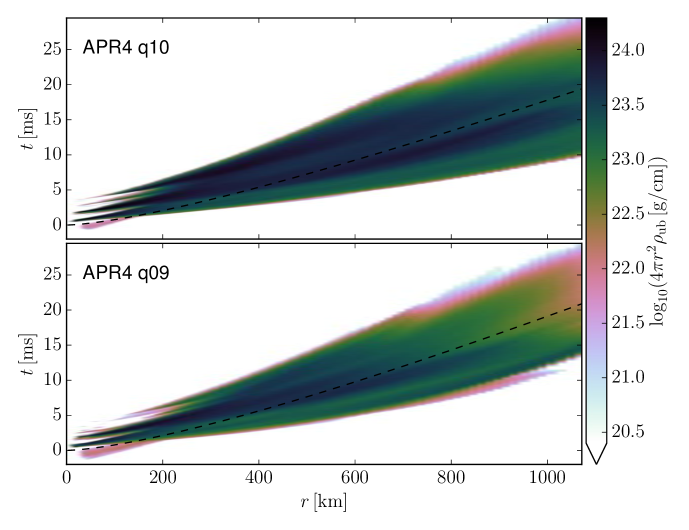
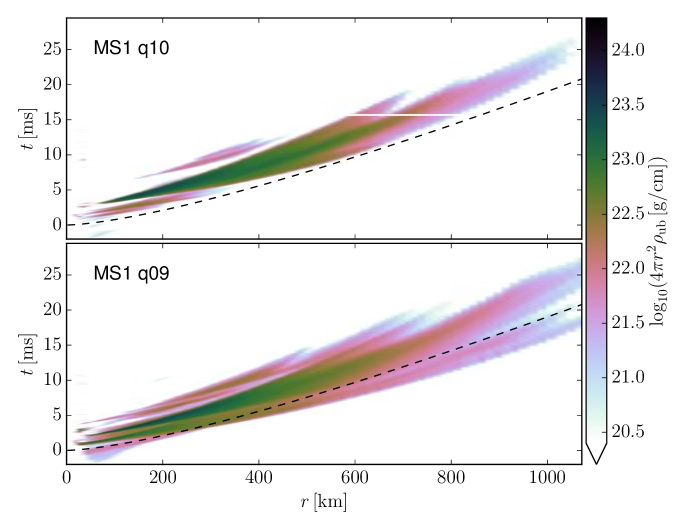
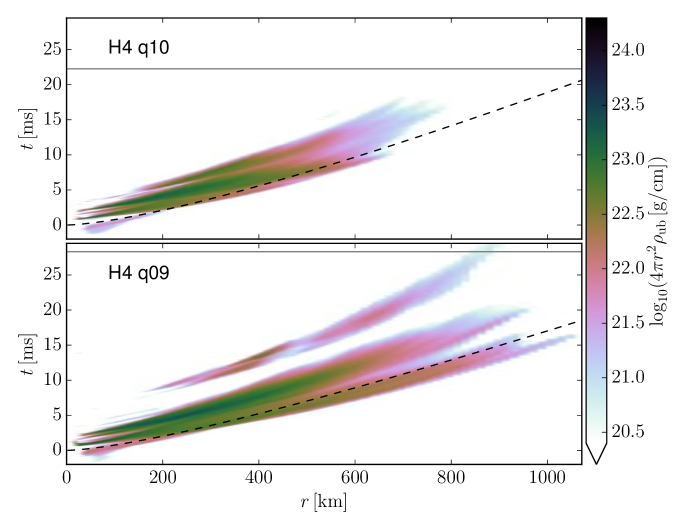
Figure 22: Radial distribution of unbound matter versus time (the white gap visible for the equal-mass MS1 model is an artifact caused by a corrupt data file). The color code corresponds to the increase of unbound mass inside spherical surfaces per increase in radius. For comparison, we also show the trajectory of a radially outgoing test mass with the escape velocity reported in Table 2, estimated using Newtonian potential of a point mass corresponding to the ADM mass at the end of the simulation. Horizontal grey lines in the H4 panels mark the collapse to black hole.

In order to judge more directly the impact of the magnetic field on this dynamic ejecta, we compare our APR4 equal-mass simulation to the corresponding unmagnetized case. Those two models were evolved with same the code, grid setup, and artificial atmosphere, and the ejected mass was extracted with the same method. The only remaining error of the differences between the two cases is the discretization error. In this respect, we note that the difference between standard and high-resolution runs (see Table 2) is around $3\%$. For the unmagnetized case, we find an ejecta mass of $0.0126\usk M_{\odot}$, i.e. a difference around $4\%$ to the magnetized case (at the same resolution). In conclusion, within the numerical error we observe no impact of the magnetic field for this model.

To investigate the ejection mechanisms, we collect the unbound matter at regular time intervals during the simulation in 1D histograms binned by radial coordinate. From this, we produce spacetime diagrams of the ejection, shown in Fig. 22. For all models, matter is ejected in several distinct waves and, with the exception of the equal-mass MS1 case, the first wave consists of material tidally ejected during merger. This can also be seen in the leftmost panels of Figures 2 to 4, showing the regions of unbound matter at merger. Not surprisingly, Fig. 22 shows that our unequal-mass models tidally eject more mass than the equal-mass ones.

The second wave is more isotropic, as can be seen in Fig. 5, and is likely the results of shock waves caused by the merger. Note that, although the breakout shock contributes significantly to the ejecta, there are further waves visible in Fig. 22 (see also the discussion in Hotokezaka et al. (2013b); Bauswein et al. (2013)). This sequence of non-tidal ejections also explains how the equal-mass APR4 model can eject more matter than the unequal-mass one. For the APR4 equal-mass case, the quasi-radial remnant oscillations are also stronger compared to the unequal-mass case, which provides a natural explanation for the higher non-tidal mass ejection.

Interestingly, the unequal-mass H4 model exhibits a wave emitted a few milliseconds after the previous ones, which is not present for the equal-mass case. We recall that those two models also showed differences in the evolution of the vortex structure (cf. Sec. IV). This last wave becomes unbound at a relatively large radius of $200\usk\mathrm{k}\mathrm{m}$. Extrapolating back to the remnant, it seems plausible that the rearrangement of the remnant fluid flow starting at $t\approx 5\usk\mathrm{m}\mathrm{s}$ (see Sec. IV) launches a wave that unbinds material in the disk.

To estimate the escape velocity, we compute the volume integrals

$$W_{\infty} =\frac{1}{M_{u}}\int u_{t}W\rho_{u}\mathrm{d}V, M_{u} =\int W\rho_{u}\mathrm{d}V$$ (2)

where $\rho_{u}$ is the density of unbound matter in the fluid rest frame, $W$ the Lorentz factor, and $\mathrm{d}V$ the proper volume element. The integral is carried out over the computational domain outside a radius of $150\usk\mathrm{k}\mathrm{m}$ and $W_{\infty}$ is evaluated at the time where $M_{u}$ becomes maximal. The average velocity of ejected matter at infinity then becomes $v_{\text{esc}}=\sqrt{1-W_{\infty}^{-2}}$. The results listed in Table 2 are of the order of $0.1\usk c$. As a cross check, we also computed for each model the trajectory of a radially outgoing test mass with the average escape velocity of the ejected matter. The results shown in Fig. 22 agree well with the ejecta, although the latter naturally show a large spread.

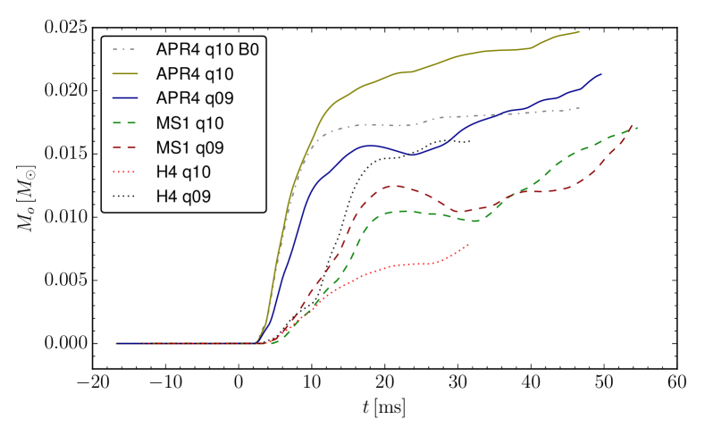
Figure 23: Cumulative outflow of matter through spherical surfaces with radius of $295\usk\mathrm{k}\mathrm{m}$ for all models.

As noted in Section III, in the post-merger phase there is also an outflow of matter that is bound according to the geodesic criterion (cf. Figures 6 to 8). In order to measure the corresponding mass flux, we compute the cumulative flux of all matter through a spherical surface with a radius of $295\usk\mathrm{k}\mathrm{m}$. Fig. 23 shows the result for the different models. The flux is largest in the first ${\approx}15\usk\mathrm{m}\mathrm{s}$ after merger, but also at later time we observe a net outflow. We also note that at $295\usk\mathrm{k}\mathrm{m}$ distance, there is no flux of unbound matter after $t\!\approx\!10\usk\mathrm{m}\mathrm{s}$ (see Fig. 22), and thus all the subsequent outflow accumulated is bound, at least according to the geodesic criterion. For the long-lived NS cases, the system tends to approach a continuous outflow towards the end of the simulation, with rates around ${\sim}0.2$–$0.3\usk M_{\odot}\mathrm{/}\mathrm{s}$.

Table 3: Properties of kilonova/macronova transients associated with the dynamical ejecta of our BNS mergers, estimated from a simple analytical model given in Grossman et al. (2014) (see text). $t_{\mathrm{k-m}}$, $L_{\mathrm{k-m}}$, and $T_{\mathrm{k-m}}$ are rough estimates for the peak time, bolometric luminosity and effective temperature of the signal. The values for the APR4 model are taken from the high-resolution run.

Model	APR4 equal	APR4 unequal	MS1 equal	MS1 unequal	H4 equal	H4 unequal
$t_{\mathrm{k-m}}\,[\mathrm{days}]$	$16$	$4.2$	$1.4$	$1.5$	$1.2$	$1.4$
$L_{\mathrm{k-m}}\,[10^{40}\,\mathrm{erg\,s}^{-1}]$	$3.1$	$2.2$	$1.0$	$1.1$	$1.0$	$1.3$
$T_{\mathrm{k-m}}\,[10^{3}\,K]$	$2.1$	$2.3$	$3.3$	$3.3$	$3.4$	$3.1$

For magnetized models, it is natural to ask if the observed outflow is magnetically driven. If this was the case, the geodesic criterion is invalid and also some of the formally bound material might escape the system, constituting a baryon-loaded wind. To answer this question, we compare the equal-mass APR4 model to the corresponding non-magnetized (but otherwise identical) model. The outflows shown in Fig. 23 are very similar until around $10\usk\mathrm{m}\mathrm{s}$ after merger. After this time, however, the outflow for the magnetized model is significantly larger, with a flux about three times larger (${\approx}0.16\usk M_{\odot}/\mathrm{s}$ compared to ${\approx}0.06\usk M_{\odot}/\mathrm{s}$ of the non-magnetized case). The cumulative outflow before this time is comparable to the ejected mass $M_{\text{ej}}$, i.e. the outflow is dominated by dynamic ejecta, while the subsequent outflow is formally bound. We also recall that although the outflowing matter is not magnetically dominated, the magnetic pressure at a radius $r=100\usk\mathrm{k}\mathrm{m}$ reaches around $0.1$ of the gas pressure (cf. Fig. 21), and therefore some influence on the dynamics of the outflows should be expected. We conclude that, in the long-lived NS cases (APR4 and MS1), the main contribution to the matter outflows observed towards the end of our simulations ($t\!>\!20\usk\mathrm{m}\mathrm{s}$) is magnetically driven. We stress that we have no indication on whether these outflows correspond to matter that will remain bound and eventually fall back onto the central NS, or escape to infinity as a baryon-loaded wind.

Neutrino emission and reabsorption, not considered in our present simulations, represent an additional mechanism to produce nearly isotropic baryon-loaded outflows Dessart et al. (2009). Therefore, properly accounting for neutrino emission would likely enhance the post-merger mass ejection reported here.

Electromagnetic counterparts from dynamical ejecta. As pointed out in the Introduction, the ejecta of BNS mergers represent very promising sites for r-process nucleosynthesis and might provide an important contribution to the heavy element abundances observed in the local universe (e.g., Just et al. (2015); Wu et al. (2016); Roberts et al. (2017)). Moreover, the radioactive decay of these elements is expected to power a late-time EM transient, a so-called kilonova or macronova, which is among the most promising EM counterparts to the GW signal from BNS mergers Li and Paczyński (1998); Kulkarni (2005); Rosswog (2005); Metzger et al. (2010); Roberts et al. (2011); Barnes and Kasen (2013); Piran et al. (2013); Tanvir et al. (2013); Berger et al. (2013); Yang et al. (2015).

Although a proper analysis is beyond the scope of this work, we can use a simple analytical model by Grossman et al. Grossman et al. (2014) to provide a rough, order-of-magnitude estimate of the peak time, peak bolometric luminosity and effective temperature of kilonova/macronova transients corresponding to the BNS mergers under investigation (we refer to Grossman et al. (2014) for a discussion on the limitations of the model):

$$t_{\mathrm{k-m}} = 4.9\,\bigg{(}\frac{M_{\mathrm{ej}}}{10^{-2}M_{\odot}}\bigg{)}^{\!1/2}\bigg{(}\frac{v_{\mathrm{esc}}}{0.1\,c}\bigg{)}^{\!-1/2}\,\mathrm{days}\,,$$

$$L_{\mathrm{k-m}} = 2.5\,\times 10^{40}\bigg{(}\frac{M_{\mathrm{ej}}}{10^{-2}M_{\odot}}\bigg{)}^{\!1-\alpha/2}\bigg{(}\frac{v_{\mathrm{esc}}}{0.1\,c}\bigg{)}^{\!\alpha/2}\,\mathrm{erg\,s}^{-1}\,,$$

$$T_{\mathrm{k-m}} = 2200\,\bigg{(}\frac{M_{\mathrm{ej}}}{10^{-2}M_{\odot}}\bigg{)}^{\!-\alpha/8}\bigg{(}\frac{v_{\mathrm{esc}}}{0.1\,c}\bigg{)}^{\!(\alpha-2)/8}\,K\,.$$

The above formulas are obtained from Grossman et al. (2014) by fixing the ejecta opacity to the fiducial value $\kappa=10\,\mathrm{cm}^{2}\,g^{-1}$ Barnes and Kasen (2013). Moreover, we set $\alpha=1.3$ as in Grossman et al. (2014). Note that here we are only considering the contribution from the dynamical ejecta that are formally unbound in our simulations. Further mass outflows (including magnetically/neutrino driven winds) can also contribute to the kilonova/macronova emission, although with a higher effective temperature and shorter timescale due to the lower opacity Metzger and Fernández (2014); Grossman et al. (2014).

Results are given in Table 3. We find the MS1 and H4 models, both with equal and unequal mass, to have similar estimates for the kilonova/macronova parameters: peak time of $\sim\!1$ day, peak luminosity of $\sim\!10^{40}$ $\mathrm{erg\,s}^{-1}$, and effective temperature around 3000 $K$. The APR4 models eject instead around one order of magnitude more mass (see Table 2 and Fig. 22), which results in much longer timescales, higher luminosity, and slightly lower effective temperature. In this case, equal- and unequal-mass models also show appreciable differences, in particular in the peak time (16 days and 4 days for the equal- and unequal-mass models, respectively).

As a final note, we recall that the interaction of the ejecta with the interstellar medium can also produce an EM transient via non-thermal synchrotron emission, which typically falls in the radio band and emerges on much longer timescales, up to $\sim$ years Nakar and Piran (2011).

VIII GW emission

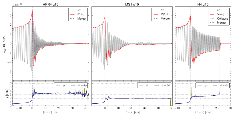
Figure 24: Gravitational wave signal for the equal-mass APR4, MS1, and H4 models (from left to right). Top panels: the thin gray lines show the strain amplitude $h^{+}_{22}$ at $100\usk\mathrm{M}\mathrm{pc}$, the red line the real part of the complex amplitude $h_{a}$ (see text). Bottom panels: the phase velocity of the complex strain $h_{22}$ before and after correcting for phase jump contributions (in yellow and blue, respectively). Note the phase velocity after $30\usk\mathrm{m}\mathrm{s}$ is not meaningful due to the low amplitude and lack of a clearly dominant mode. The vertical lines mark the times of merger (dashed) and of black hole formation (dotted).

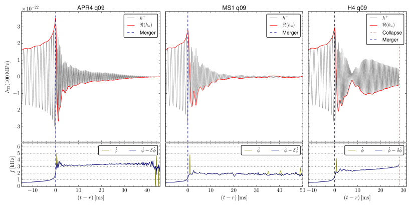
Figure 25: Like Fig. 24, but showing the unequal-mass models. Note that the H4 unequal-mass model formed a black hole (vertical dotted line), but the simulation was not carried on for long enough to extract the gravitational wave signal of the collapse.

In this Section, we conclude our analysis by discussing the GW emission of our BNS mergers. For all our simulations, we extract the GW strain from the Weyl scalar $\Psi_{4}$ at a fixed radius of $1181\usk\mathrm{k}\mathrm{m}$, without extrapolating to infinity. The numerical accuracy is discussed in the Appendix. The GW strains given in the following are the coefficients of the decomposition into spin-weighted spherical harmonics ${}_{-2}Y_{lm}$, and the strain at a particular viewing angle can be obtained by multiplication with $\left|{}_{-2}Y_{lm}(\theta,\phi)\right|$. For the time integration, we developed a new method which is described in Kastaun et al. (2016b); the advantage is that the improved removal of offsets results in centered waveforms also for low-amplitude parts, i.e. minima and tails.

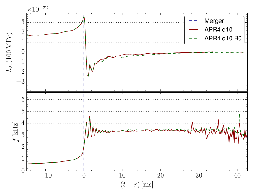
Figure 26: Comparison of gravitational wave strain $\Re(h_{a})$ (top panel) and jump-corrected phase velocity (bottom panel), between the magnetized APR4 equal-mass model and the corresponding non-magnetized model.

More importantly, we also employ a scheme to detect phase jumps caused by over-modulation. This term denotes signals in the form $A(t)e^{i\phi(t)}$, where $A\in\mathbb{R}$ is slowly changing compared to $\phi$, but can have zero crossings. A sign change of $A$ then corresponds to a phase jump by $\pi$ of the signal. More generally, if $A$ is complex valued a rapid phase change occurs when $A$ passes close to the origin in the complex plane. Our scheme decomposes the complex-valued strain amplitude $h=h^{+}-ih^{\times}$ as $h(t)=h_{a}(t)e^{i\phi(t)}$, such that $h_{a}$ has a significant imaginary part only near phase jumps, and a real part that can cross zero. This is expressed by a phase correction $\delta\phi$, with $h_{a}(t)=|h(t)|e^{-i\delta\phi(t)}$. For further details of the method, we refer to Kastaun et al. (2016b).

The GW strain and the phase velocity for all magnetized models are shown in Figures 24 and 25. In addition, we visualize the phase jumps using the real part of $h_{a}$ and the jump-corrected phase velocity. All models show the characteristic amplitude minimum seen at merger in many BNS simulations. Using our heuristic phase jump detection, we find that those minima are caused by over-modulation. This is clearly visible in the phase velocities, which exhibit a sharp peak (coincident with the time of the amplitude minimum) before subtracting the correction $\delta\phi$. This observation is relevant for GW astronomy, where the data analysis is very sensitive to the phasing. For all the cases at hand, the phase around merger can be well described by two relatively smooth parts separated by a rapid jump by $\pi$. The phase velocity at merger, i.e. at the time of maximum strain amplitude, is given in Table 2. The jump-corrected phase velocity can still show a modulation lasting a few ms after merger (most evident in the APR4 equal-mass case). This is most likely caused by quasi-radial oscillations, which we also observe in the maximum density.

After merger, the instantaneous GW frequency increases slightly and slowly for the APR4 models, and remains almost constant for the MS1 models. For the H4 models, it increases significantly until the system starts collapsing into a BH. For the equal-mass model, the frequency quickly increases to $4\usk\mathrm{k}\mathrm{Hz}$ at the time of the collapse. For the unequal-mass H4 model, the simulation was ended before the signal of the collapse reached the extraction radius. For the cases at hand, we find that the frequency drift becomes larger the closer the remnant is to the collapse threshold.

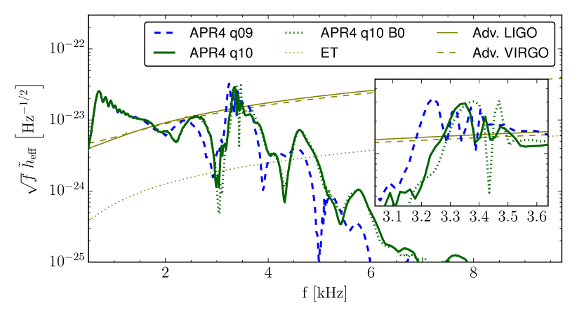
Figure 27: Power spectrum of the gravitational wave strain at $100\usk\mathrm{M}\mathrm{pc}$ for the APR4 models, compared to the sensitivity curves of current and planned gravitational wave detectors.

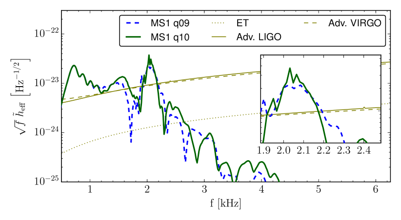
Figure 28: Like Fig. 27, but for the MS1 models.

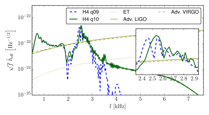
Figure 29: Like Fig. 27, but for the H4 models. Note the differences in the high-frequency part are simply due to the fact that the unequal-mass case was not evolved long enough to obtain the part of the signal corresponding to the collapse to a black hole.

In terms of post-merger waveforms, long-lived remnants (APR4, MS1 EOS) are characterized by comparable amplitudes that decay significantly within $10$–$20\usk\mathrm{m}\mathrm{s}$. The HMNS cases (H4 EOS) have instead a stronger and more persistent emission until the sudden drop of amplitude associated with the collapse. The largest difference between equal and unequal-mass cases is also found for the H4 EOS. The amplitude for mass ratio $q=0.9$ shows a pronounced second minimum, while for the equal-mass model it decreases monotonically. One possible explanation for this general type of behavior would be the excitation of an unstable oscillation mode while the original mode excited during merger is damped. This seems unlikely since the phase velocity remains smooth, which would not be the case when two different modes with comparable amplitude are present at the same time. Another possibility is that the original mode becomes unstable due to an increase of compactness and frequency. This is also unconvincing since the mode frequencies span the same range for both mass ratios. In case of a CFS unstable mode, the inertial-frame frequency should also be small near the critical rotation rate.

We favor an explanation recently proposed in Kastaun et al. (2016b), namely that the density deformation is partly due to vortices in the fluid flow, and that these can undergo both smooth and sudden rearrangements. This could also explain smaller irregularities of the strain amplitude. The hypothesis is not proven, in particular it is possible that vortex rearrangements and frequency changes have a common cause instead. However, as discussed in Sec. IV, we do see for the H4 unequal-mass case a clear rearrangement of the remnant structure in the frame corotating with the $m=2$ density deformation (cf. Fig. 11). Also, we found that the contributions of the outer layers and the core to the quadrupole moment have opposite sign. This might lead to cancellation effects amplifying the impact of rearrangements on the GW amplitude.

The effect of the magnetic field on GW strain and phase velocity is shown in Fig. 26 for the equal-mass APR4 model. We find very little difference in this case. Note that the impact for a remnant closer to collapse could be larger since near the threshold for BH formation the system tends to be very sensitive to small changes. In particular, the lifetime of the remnant could be altered significantly.

The Fourier spectra of the GW signals are shown in Figures 27 to 29, each comparing the equal- and unequal-mass models for one EOS. The main peak caused by the post-merger phase shows only minor changes for different mass ratios, compared to the width of the peak. The impact of the EOS exceeds by far that of the mass ratio, at least in the range $q\!=\!0.9$ to $1$. We note that a small influence of the mass ratio makes it easier to constrain the EOS from the post-merger frequency. Correlations between EOS, initial NS properties, and post-merger frequencies have been studied by different groups, e.g. Bauswein and Janka (2012); Bernuzzi et al. (2015); Rezzolla and Takami (2016), for a large number of models.

In all cases, the post-merger peak as well as the inspiral contribution are above the (design) sensitivity curves of the advanced LIGO and Virgo detectors. Nevertheless, the corresponding signal-to-noise ratio (SNR) is likely insufficient for a confident detection of the post-merger signal at $100\usk\mathrm{M}\mathrm{pc}$ distance. Of the three EOS, the APR4 EOS leads to the post-merger signal with the smallest SNR. Although the H4 models emit the strongest post-merger signals (see discussion above), their frequency is also higher, such that the MS1 and H4 cases result in comparable SNRs.

The dominant frequency of the post-merger phase for each model is given in Table 2. We report both the location $f_{\mathrm{pm}}$ of the maximum in the Fourier spectrum as well as a measure defined in Hotokezaka et al. (2013c) using the instantaneous frequency $f$ to compute

$$f_{10} =\left(\int|h(t)|\,\mathrm{dt}\right)^{-1}\int f(t)|h(t)|\,\mathrm{dt},$$ (3)

where the time integrals are carried out over the first $10\usk\mathrm{m}\mathrm{s}$ after merger. Interestingly, the GW frequency in the post-merger phase is approximately twice the maximum rotation rate inside the remnant (compare $2\nu_{\mathrm{max}}$ and $f_{\mathrm{pm}}$ in Table 2, as well as Fig. 15). As was already observed in Kastaun and Galeazzi (2015); Endrizzi et al. (2016); Kastaun et al. (2016a, b); Hanauske et al. (2016), the maximum rotation rate is apparently limited by the angular velocity of the $m=2$ density deformation, which is in turn half of the GW frequency. The frequency of the main post-merger peak increases with the bulk compactness of the remnant (as does the rotation rate, see Sec. IV), which depends on the EOS.

When considering the characteristic low- and high-frequency side peaks appearing around the main post-merger peak, we find more significant differences between the equal and unequal-mass cases. We caution however that those peaks are not necessarily related directly to physical oscillations. As was already shown in Kastaun et al. (2016b), their location can change drastically when removing the aforementioned phase jumps. This can be explained in terms of cancellations between the contributions of different parts of the signal to the Fourier spectrum.

The impact of the magnetic field on the spectrum is rather small, as shown in Fig. 27. We observe a slight shift of the main peak, which is however less than the peak width. The sub-structure of the peak also changes slightly, such that a sub-peak at $3.47\usk\mathrm{k}\mathrm{Hz}$ becomes the new global maximum for the non-magnetic case. The average frequency $f_{10}$ changes less than $0.5\%$. Also the amplitude of the peak and the corresponding SNR is essentially unaffected by the magnetic field. Overall, we conclude that magnetic fields up to the strength considered here are unlikely to cause any detectable changes in the GW signal for BNS mergers forming a long-lived NS.

IX Summary and Conclusions

In this paper, we investigated the merger of BNS systems by means of GRMHD simulations, with special attention devoted to mergers producing a long-lived NS remnant (i.e. a supramassive or stable NS). We considered equal and unequal mass binaries with mass ratios $q=1$ and $0.9$, keeping a fixed total gravitational mass at infinity of $2.7\usk M_{\odot}$. We considered three different EOS known in the literature: APR4, MS1, and H4. For the given total mass, these EOS lead to the formation of supramassive, stable, and hypermassive NS remnants, respectively. Only the latter models (H4 EOS) collapse to a BH by the end of our simulations, which cover the evolution up to ${\sim}30$–$50$ ms after merger.

Remnant structure, rotation profile, accretion disk. We studied in detail the structure and the fluid flow of the merger remnants. In a frame corotating with the dominant $m=2$ density deformation, the remnant structure appears much more complex than simple differential rotation. In particular, we found long-standing vortices correlated with density perturbations, which slowly evolve towards axisymmetry. In the H4 unequal-mass case, we also found a sudden rearrangement of the internal flow starting $\sim 5$ ms after merger, which seems to have an impact on the HMNS lifetime and to leave a distinctive signature on GW signal and mass ejection.

For the long-lived models, a quasi-stationary state is reached around $20\usk\mathrm{m}\mathrm{s}$. For all models, the rotation profiles on the equatorial plane around this time shows a generic structure with a slowly rotating core, a maximum rotation rate at a radius of ${\sim}15$–$20\usk\mathrm{k}\mathrm{m}$, and an approximately Keplerian rotation profile in the outer layers. This confirms previous indications suggesting that the collapse is not prevented by a rapidly rotating core, but rather by the centrifugal support of the outer layers of the remnant. The EOS is found to have a much stronger impact than the mass ratio on the maximum angular velocity, which is approximately given by the angular velocity of the $m=2$ density perturbation. Moreover, we found that the slowly rotating core is well approximated by the core of a TOV (i.e. non-rotating NS) solution and that BNS merger remnants seem to resist the collapse as long as a TOV core equivalent is admitted. Our H4 models indeed collapse to BH as soon as this condition is no longer satisfied.

For our collapsing (H4) models, we found BHs with spin parameter of ${\sim}0.6$ surrounded by accretion disks of $0.1-0.2\usk M_{\odot}$. In the long-lived NS cases (APR4 and MS1), we found a significant amount of mass outside the remnant at radii $r>20\usk\mathrm{k}\mathrm{m}$: $\sim 0.2$ and $\sim 0.4\usk M_{\odot}$ for the APR4 and MS1 models, respectively (roughly half of which outside a radius of $60$ km). We note that further away from the remnant the matter is distributed more isotropically (i.e. also along the orbital axis) and its internal flow is rather unordered and does not correspond to simple accretion, at least on the timescales covered by our simulations (${\sim}50$ ms after merger). We also note that a small fraction of this mass will be ejected from the system. As a general trend, unequal-mass systems are found to produce more massive disks (by ${\sim}25$% in the long-lived NS cases, and ${\sim}60$% in the collapsing cases).

Magnetic fields. The evolution of magnetic fields is characterized by different stages of amplification. We started from initial poloidal fields of ${\sim}10^{15}$ G confined inside the two NSs and we observed a first stage of amplification taking place already before merger. Interestingly, all models started with the same total magnetic energy and gravitational mass at infinity, and all ended up with roughly the same magnetic energy at the time of merger, which is about one order of magnitude higher than the initial one. Nevertheless, it is still unclear whether this amplification corresponds to a well-resolved physical mechanism, although our analysis ruled out a number of physical and numerical causes. A possible explanation might be that the time-changing tidal deformations during inspiral induce fluid flows inside the two NSs that might amplify the magnetic field. This effect will be further investigated in future studies.

After merger, magnetic fields are strongly amplified for $5$–$10\usk\mathrm{m}\mathrm{s}$, most likely by the KH instability. Further amplification continues at later times, although at a lower rates. In this last phase, the MRI outside the NS remnant is likely playing a major role in the amplification. From our resolution study, it is clear that the KH phase is not well resolved. However, the magnetic energy achieved in last stage (up to ${\sim}50\usk\mathrm{m}\mathrm{s}$ after merger for the long-lived NS models) shows a much better convergence.

The overall dependence on EOS and mass ratio is non-trivial and no general trend is observed. At all stages, the magnetic field amplification is mostly in the toroidal component and takes place mostly on the equatorial plane. We studied the geometrical distribution of magnetic fields in 3D for the long-lived NS cases, and found that no ordered configuration has emerged around the orbital axis by the end of our simulations, although we note a slight tendency to helical structures.

Short gamma-ray bursts. We discussed how our results compare with different scenarios linking BNS mergers to the central engine of SGRBs. In particular, we considered the leading BH-disk scenario and the alternative magnetar scenario. Both models envisage the formation of an accretion-powered jet launched by the post-merger system, i.e. a BH surrounded by a massive accretion disk in the former case and a strongly magnetized long-lived NS also surrounded by an accretion disk in the latter case. While not much can be added on the standard BH-disk scenario from our collapsing (H4) models, since the simulations were interrupted only a few ms after BH formation, our long-lived NS (APR4 and MS1) models provided useful indications on the viability of the magnetar scenario. We note that so far this case has been poorly investigated in numerical relativity, with only very few studies reporting on GRMHD simulations of BNS mergers with long-lived NS remnants. We found that $\sim 50$ ms after merger, the long-lived NS is still surrounded by a dense and nearly isotropic environment. In particular, baryon pollution along the orbital axis is substantial (densities of $\sim 10^{10}$ g/cm³) and could easily prevent the formation of an incipient jet. In addition, there is no well defined accretion flow nor an ordered magnetic field structure that could favor the launch of a collimated outflow. We thus concluded that the long-lived NS systems considered are not able to produce a jet, at least on timescales of $\sim 0.1$ s. As we discussed, however, such a conclusion could be affected by our present limitations.

Matter ejection. We carried out a detailed analysis of the matter ejected during and after merger. We estimated the outflow of matter that is unbound according to the geodesic criterion and we found dynamical ejecta composed by (i) initial tidal tails launched right before merger that are more massive for the unequal-mass models, (ii) a strong ejecta wave, most likely due to the breakout shock generated when the two NS cores collide, and (iii) additional ejecta waves launched by the first oscillations of the remnant NS. In total, these ejecta amount to $\sim 10^{-2}\usk M_{\odot}$ for the APR4 models and $\sim 10^{-3}\usk M_{\odot}$ for the others . Within the errors, magnetic fields have negligible effect on these results. Using a simple analytical model by Grossman et al. (2014), we also obtained order-of-magnitude estimates for the corresponding kilonova/macronova signals. We found electromagnetic transients peaking around $1$–$10$ days after merger, with peak luminosities of ${\sim}10^{40}$ erg/s and effective temperatures of ${\sim}2000$–$3000$ K.

In addition to the formally unbound ejecta, we observed further matter outflows. These become dominant $15$–$20\usk\mathrm{m}\mathrm{s}$ after merger and, although slower, they can contribute significantly to the total flux accumulated by the end of the simulations across a spherical surface of radius ${\approx}300\usk\mathrm{k}\mathrm{m}$. In particular, for the long-lived NS cases ${\sim}50\usk\mathrm{m}\mathrm{s}$ after merger, the cumulative flux of formally bound matter can be comparable to the unbound ejecta (APR4) or even dominant (MS1). Moreover, by comparing results obtained with and without magnetic fields, we found that the main contribution to these outflows is magnetically driven. This indicates that the geodesic criterion does not apply and leaves the possibility that a relevant fraction of this matter could also become unbound at later times. Finally, our simulations suggest that the ongoing matter ejection will persist for much longer.

Gravitational wave emission. For all our models, we analyzed the GW signal, with particular attention to the post-merger waveform and spectrum. Systems forming a long-lived NS (APR4 and MS1 models) have post-merger waveforms of similar amplitudes which rapidly decay within ${\sim}20\usk\mathrm{m}\mathrm{s}$. The collapsing (H4) models show a stronger post-merger GW emission that is however shut off as soon as the HMNS collapses to a BH. We note that all models exhibit a phase jump during merger, which might be relevant for GW analysis. In agreement with well established results in the literature, we found post-merger spectra characterized by a main peak at a frequency of $2$–$3$ kHz. While the mass ratio has minor influence on this frequency, differences are significant for different EOS. In particular, more compact remnants have a higher peak frequency. We recall that all our BNS systems have the same total mass at infinite separation. By comparing the spectra of the magnetized and non-magnetized APR4 equal-mass models, we concluded that for BNS merger forming a long-lived NS, magnetic fields up to $\sim 10^{16}$ G are unlikely to alter the GW spectrum in a detectable way.

Although for all our models the main post-merger peak lies above the sensitivity curves of advanced LIGO and Virgo, the SNRs are most probably not sufficient for a confident detection of the post-merger part of the GW signal at a distance of $\sim 100$ Mpc or more.

Outlook. With the present work, we initiated a systematic investigation of BNS mergers leading to the formation of a long-lived NS. As suggested by recent observations, this case might represent a significant fraction of all BNS mergers. Nevertheless, it remains poorly studied in numerical relativity and thus more effort in this direction is urgently needed.

The results presented here are affected by various limitations that should be overcome step by step in the future. In particular, a higher resolution is needed to better resolve the KH instability and possibly the MRI also inside the remnant. Moreover, an improved description of the microphysics including composition and neutrino radiation is likely to affect the structure of the NS remnant and surrounding disk/environment, and the matter outflows. Both improvements are also required to make conclusive statements about jet formation.

See Supplemental Material at http://link.aps.org/ ​supplemental/10.1103/PhysRevD.95.063016 for initial data (LORENE input/ouput files) and data files of the obtained gravitational waveforms.

Appendix: Resolution study

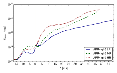
Figure 30: Evolution of magnetic energy for the equal-mass APR4 model at different resolutions: low resolution $dx=277\usk\mathrm{m}$ (LR), fiducial/medium resolution $dx=222\usk\mathrm{m}$ (MR), and high resolution $dx=177\usk\mathrm{m}$ (HR). The vertical line marks the time of merger.

In order to estimate the numerical errors, we evolved the equal-mass APR4 model with two additional resolutions, one higher and one lower by a factor $1.25$ than the fiducial (medium) resolution. The corresponding spacing of the finest grids is $277,222$, and $177\usk\mathrm{m}$. First, we compute the error of the maximum rest-mass density during the evolution. We define the difference between two resolutions as

$$\delta_{\rho}\equiv\frac{\int\left(\rho_{1}\left(t\right)-\rho_{2}\left(t\right)\right)^{2}\,\mathrm{d}t}{\int\frac{1}{4}\left(\rho_{1}\left(t\right)+\rho_{2}\left(t\right)\right)^{2}\,\mathrm{d}t},$$ (4)

where the integrals are carried out over the full duration of the simulations, and the time coordinates are aligned at the time of the merger for each run. We obtain relative differences of $\delta_{\rho}\approx 3.5\%$ between low and medium resolution and ${\approx}1.0\%$ between medium and high resolution. This would correspond to a convergence order of $5.7$. Similarly, the minimum of the lapse would converge with order $4.6$. Nevertheless, both convergence orders are clearly misleading, since the hydrodynamic evolution scheme is second order accurate at best, and in practice between first and second order due to the presence of shock waves. In the following, we provide error estimates under the assumption that only the lowest resolution is too low and that results show first order convergence starting from medium resolution.

We now estimate the error on the GW frequencies for the APR4 case. The average post-merger frequency $f_{10}$ differs by $0.31\%$ between low and medium resolution, and by $0.24\%$ between medium and high resolution. From the latter results and the above assumption of linear convergence, we estimate the error of $f_{10}$ to be below $2\%$. We also note that the frequency range relevant for our results (up to $4\usk\mathrm{k}\mathrm{Hz}$) corresponds to wavelengths resolved by at least 10 grid points at the extraction radius, which is sufficient to prevent signal loss.

Our MS1 and H4 equal-mass models have also been studied in Hotokezaka et al. (2013c), using the same piecewise polytropic approximation of the EOS and the same thermal part, but without magnetic fields. Assuming that the impact of the magnetic field is as small as for the APR4 case, we expect to obtain similar frequencies. For those models, the post-merger frequency $f_{10}$ indeed agrees within $1.3\%$ and $0.4\%$, respectively. Our unmagnetized APR4 equal-mass model is almost the same as another model studied in Hotokezaka et al. (2013c), apart from a slightly different piecewise polytropic approximation (see Endrizzi et al. (2016)) of the APR4 EOS used in our work. For this model, $f_{10}$ agrees within $1.5\%$. We conclude that within the numerical error and neglecting the influence of magnetic fields, our results agree well with Hotokezaka et al. (2013c).

Next, we consider the finite difference error in our estimates of the (unbound) ejected mass. Again, a direct measure of the convergence order yields an unrealistically large value (${\approx}10$). The difference between medium and high resolution is $3.5\%$, and under the assumption of first order convergence, we obtain a total error of $17\%$. Note, however, that this does not include the effects of the artificial atmosphere and the assumptions used in the extraction. In total, we roughly estimate the mass of the unbound ejecta to be accurate within a factor of 2.

Finally, we consider the impact of resolution on magnetic field evolution and amplification. Figure 30 shows the evolution of the total magnetic energy for low, medium and high resolution. The initial amplification during the inspiral seems to converge until the saturation phase, where the absolute differences become suddenly larger and convergence is gradually lost. This could mean that the saturation is due to the finite resolution or that a physical effect causing the saturation is more difficult to resolve. We note that a resolution study does not allow us to exclude the remote possibility that interaction with the artificial atmosphere is responsible for the amplification. As expected, in the post-merger phase we are not in a regime of convergence. This is likely due to the unresolved small-scales at which the key amplification mechanisms act (in particular the KH instability). Nevertheless, for $t>30\usk\mathrm{m}\mathrm{s}$ we find a much better agreement between the medium and high resolutions compared to the low and medium resolutions. A possible explanation is that magnetic energy in this late phase is dominated by the contributions of MRI and winding outside the remnant, which are much better resolved (as shown in Fig. 17, the resolution should be sufficient to resolve the fastest growing MRI modes).

References

- Abbott et al. (2016a) B. P. Abbott et al. (LIGO Scientific Collaboration and Virgo Collaboration), Phys. Rev. Lett. 116, 061102 (2016a).
- Abbott and et al (2016b) B. P. Abbott et al. (LIGO Scientific Collaboration and Virgo Collaboration), Phys. Rev. Lett. 116, 241103 (2016b).
- Abbott and et al (2016b) B. P. Abbott et al. (LIGO Scientific Collaboration and Virgo Collaboration), Astrophys. J. Lett. 826, L13 (2016a) .
- LIGO Scientific Collaboration et al. (2015) LIGO Scientific Collaboration, J. Aasi et al., Class. Quantum Grav. 32, 074001 (2015) .
- Accadia et al. (2011) T. Accadia et al., Class. Quantum Grav. 28, 114002 (2011).
- Abadie et al. (2010) J. Abadie, et al. Class. Quantum Grav. 27, 173001 (2010) .
- Abbott et al. (2016b) B. P. Abbott et al., Astrophys. J. Lett. 832, L21 (2016b) .
- Perna et al. (2016) R. Perna, D. Lazzati, and B. Giacomazzo, ApJ 821, L18 (2016) .
- Shibata et al. (2005) M. Shibata, K. Taniguchi, and K. Uryū, Phys. Rev. D 71, 084021 (2005) .
- Bauswein et al. (2013) A. Bauswein, T. W. Baumgarte, and H.-T. Janka, Phys. Rev. Lett. 111, 131101 (2013).
- Just et al. (2015) O. Just, A. Bauswein, R. A. Pulpillo, S. Goriely, and H.-T. Janka, Mon. Not. R. Astron. Soc. 448, 541 (2015) .
- Wu et al. (2016) M.-R. Wu, R. Fernández, G. Martínez-Pinedo, and B. D. Metzger, Mon. Not. R. Astron. Soc. 463, 2323 (2016) .
- Roberts et al. (2017) L. F. Roberts, J. Lippuner, M. D. Duez, J. A. Faber, F. Foucart, J. C. Lombardi, Jr., S. Ning, C. D. Ott, and M. Ponce, Mon. Not. R. Astron. Soc. 464, 3907 (2017) .
- Metzger and Berger (2012) B. D. Metzger and E. Berger, ApJ 746, 48 (2012) .
- Berger (2014) E. Berger, ARA&A 52, 43 (2014) .
- Metzger et al. (2014) B. D. Metzger, I. Vurm, R. Hascoët, and A. M. Beloborodov, Mon. Not. R. Astron. Soc. 437, 703 (2014) .
- Siegel and Ciolfi (2016a) D. M. Siegel and R. Ciolfi, Astrophys. J. 819, 14 (2016a) .
- Siegel and Ciolfi (2016b) D. M. Siegel and R. Ciolfi, Astrophys. J. 819, 15 (2016b) .
- Paczynski (1986) B. Paczynski, Astrophys. J. Lett. 308, L43 (1986).
- Eichler et al. (1989) D. Eichler, M. Livio, T. Piran, and D. N. Schramm, Nature 340, 126 (1989).
- Narayan et al. (1992) R. Narayan, B. Paczynski, and T. Piran, Astrophys. J. Lett. 395, L83 (1992) .
- Barthelmy et al. (2005) S. D. Barthelmy et al., Nature 438, 994 (2005) .
- Fox et al. (2005) D. B. Fox et al. , Nature 437, 845 (2005).
- Gehrels et al. (2005) N. Gehrels et al., Nature 437, 851 (2005) .
- Shibata et al. (2006) M. Shibata, M. D. Duez, Y. T. Liu, S. L. Shapiro, and B. C. Stephens, Phys. Rev. Lett. 96, 031102 (2006) .
- Tanvir et al. (2013) N. R. Tanvir, A. J. Levan, A. S. Fruchter, J. Hjorth, R. A. Hounsell, K. Wiersema, and R. L. Tunnicliffe, Nature 500, 547 (2013) .
- Berger et al. (2013) E. Berger, W. Fong, and R. Chornock, Astrophys. J. Lett. 774, L23 (2013) .
- Paschalidis et al. (2015) V. Paschalidis, M. Ruiz, and S. L. Shapiro, Astrophys. J. Letter 806, L14 (2015) .
- Ruiz et al. (2016) M. Ruiz, R. N. Lang, V. Paschalidis, and S. L. Shapiro, Astrophys. J. Lett. 824, L6 (2016) .
- Hotokezaka et al. (2013a) K. Hotokezaka, K. Kyutoku, M. Tanaka, K. Kiuchi, Y. Sekiguchi, M. Shibata, and S. Wanajo, Astrophys. J. Lett. 778, L16 (2013a) .
- Oechslin et al. (2007) R. Oechslin, H.-T. Janka, and A. Marek, Astron. Astrophys. 467, 395 (2007) .
- Bauswein et al. (2013) A. Bauswein, S. Goriely, and H.-T. Janka, Astrophys. J. 773, 78 (2013) .
- Kastaun and Galeazzi (2015) W. Kastaun and F. Galeazzi, Phys. Rev. D 91, 064027 (2015).
- Dessart et al. (2009) L. Dessart, C. D. Ott, A. Burrows, S. Rosswog, and E. Livne, Astrophys. J. 690, 1681 (2009) .
- Siegel et al. (2014) D. M. Siegel, R. Ciolfi, and L. Rezzolla, Astrophys. J. Lett. 785, L6 (2014) .
- Metzger and Fernández (2014) B. D. Metzger and R. Fernández, Mon. Not. R. Astron. Soc. 441, 3444 (2014) .
- Murguia-Berthier et al. (2014) A. Murguia-Berthier, G. Montes, E. Ramirez-Ruiz, F. De Colle, and W. H. Lee, Astrophys. J. Lett. 788, L8 (2014) .
- Nagakura et al. (2014) H. Nagakura, K. Hotokezaka, Y. Sekiguchi, M. Shibata, and K. Ioka, Astrophys. J. Lett. 784, L28 (2014) .
- Murguia-Berthier et al. (2016) A. Murguia-Berthier, E. Ramirez-Ruiz, G. Montes, F. De Colle, L. Rezzolla, S. Rosswog, K. Takami, A. Perego, and W. H. Lee, ArXiv e-prints (2016), arXiv:1609.04828 [astro-ph.HE] .
- Ciolfi and Siegel (2015a) R. Ciolfi and D. M. Siegel, Astrophys. J. Lett. 798, L36 (2015a) .
- Rezzolla and Kumar (2015) L. Rezzolla and P. Kumar, Astrophys. J. 802, 95 (2015) .
- Li and Paczyński (1998) L.-X. Li and B. Paczyński, Astrophys. J. 507, L59 (1998) .
- Kulkarni (2005) S. R. Kulkarni, ArXiv Astrophysics e-prints (2005), astro-ph/0510256 .
- Rosswog (2005) S. Rosswog, Astrophys. J. 634, 1202 (2005) .
- Metzger et al. (2010) B. D. Metzger, G. Martínez-Pinedo, S. Darbha, E. Quataert, A. Arcones, D. Kasen, R. Thomas, P. Nugent, I. V. Panov, and N. T. Zinner, Mon. Not. R. Astron. Soc. 406, 2650 (2010) .
- Roberts et al. (2011) L. F. Roberts, D. Kasen, W. H. Lee, and E. Ramirez-Ruiz, Astrophys. J. Lett. 736, L21 (2011) .
- Barnes and Kasen (2013) J. Barnes and D. Kasen, Astrophys. J. Lett. 775, 18 (2013) .
- Piran et al. (2013) T. Piran, E. Nakar, and S. Rosswog, Mon. Not. R. Astron. Soc. 430, 2121 (2013) .
- Yang et al. (2015) B. Yang, Z.-P. Jin, X. Li, S. Covino, X.-Z. Zheng, K. Hotokezaka, Y.-Z. Fan, T. Piran, and D.-M. Wei, Nature Communications 6, 7323 (2015) .
- Radice et al. (2016) D. Radice, F. Galeazzi, J. Lippuner, L. F. Roberts, C. D. Ott, and L. Rezzolla, Mon. Not. R. Astron. Soc. 460, 3255 (2016) .
- Fernández and Metzger (2013) R. Fernández and B. D. Metzger, Mon. Not. R. Astron. Soc. 435, 502 (2013) .
- Baumgarte et al. (2000) T. W. Baumgarte, S. L. Shapiro, and M. Shibata, Astrophys. J. Lett. 528, L29 (2000) .
- Shibata and Taniguchi (2006) M. Shibata and K. Taniguchi, Phys. Rev. D 73, 064027 (2006) .
- Duez et al. (2006a) M. D. Duez, Y. T. Liu, S. L. Shapiro, M. Shibata, and B. C. Stephens, Phys. Rev. D 73, 104015 (2006a) .
- Siegel et al. (2013) D. M. Siegel, R. Ciolfi, A. I. Harte, and L. Rezzolla, Phys. Rev. D 87, 121302(R) (2013) .
- Endrizzi et al. (2016) A. Endrizzi, R. Ciolfi, B. Giacomazzo, W. Kastaun, and T. Kawamura, Class. Quantum Grav. 33, 164001 (2016).
- Kastaun et al. (2016a) W. Kastaun, R. Ciolfi, and B. Giacomazzo, Phys. Rev. D 94, 044060 (2016a) .
- Kastaun et al. (2016b) W. Kastaun, R. Ciolfi, A. Endrizzi, and B. Giacomazzo, ArXiv e-prints (2016b), arXiv:1612.03671 [astro-ph.HE] .
- Hanauske et al. (2016) M. Hanauske, K. Takami, L. Bovard, L. Rezzolla, J. A. Font, F. Galeazzi, and H. Stöcker, ArXiv e-prints (2016), arXiv:1611.07152 [gr-qc] .
- Bauswein and Janka (2012) A. Bauswein and H.-T. Janka, Phys. Rev. Lett. 108, 011101 (2012) .
- Bauswein et al. (2014) A. Bauswein, N. Stergioulas, and H.-T. Janka, Phys. Rev. D 90, 023002 (2014) .
- Takami et al. (2014) K. Takami, L. Rezzolla, and L. Baiotti, Phys. Rev. Lett. 113, 091104 (2014) .
- Demorest et al. (2010) P. B. Demorest, T. Pennucci, S. M. Ransom, M. S. E. Roberts, and J. W. T. Hessels, Nature 467, 1081 (2010) .
- Antoniadis et al. (2013) J. Antoniadis et al., Science 340, 448 (2013) .
- Lasota et al. (1996) J.-P. Lasota, P. Haensel, and M. A. Abramowicz, Astrophys. J. 456, 300 (1996) .
- Belczynski et al. (2008) K. Belczynski, R. O’Shaughnessy, V. Kalogera, F. Rasio, R. E. Taam, and T. Bulik, Astrophys. J. Lett. 680, L129 (2008) .
- Giacomazzo and Perna (2013) B. Giacomazzo and R. Perna, Astrophys. J. Lett. 771, L26 (2013) .
- Palenzuela et al. (2015) C. Palenzuela, S. L. Liebling, D. Neilsen, L. Lehner, O. L. Caballero, E. O’Connor, and M. Anderson, Phys. Rev. D 92, 044045 (2015) .
- Gehrels et al. (2004) N. Gehrels et al., Astrophys. J. 611, 1005 (2004).
- Rowlinson et al. (2013) A. Rowlinson, P. T. O’Brien, B. D. Metzger, N. R. Tanvir, and A. J. Levan, Mon. Not. R. Astron. Soc. 430, 1061 (2013) .
- Lü et al. (2015) H.-J. Lü, B. Zhang, W.-H. Lei, Y. Li, and P. D. Lasky, Astrophys. J. 805, 89 (2015) .
- Yu et al. (2013) Y.-W. Yu, B. Zhang, and H. Gao, Astrophys. J. Lett. 776, L40 (2013) .
- Dai et al. (2016) Z. G. Dai, J. S. Wang, and X. F. Wu, ArXiv e-prints (2016), arXiv:1611.09517 [astro-ph.HE] .
- Lattimer (2012) J. M. Lattimer, Annu. Rev. Nucl. Part. Sci. 62, 485 (2012).
- Özel and Freire (2016) F. Özel and P. Freire, Ann. Rev. Astron. Astrophys. 54, 401 (2016) .
- Akmal et al. (1998) A. Akmal, V. R. Pandharipande, and D. G. Ravenhall, Phys. Rev. C 58, 1804 (1998).
- Müller and Serot (1996) H. Müller and B. D. Serot, Nucl. Phys. A 606, 508 (1996) .
- Glendenning and Moszkowski (1991) N. K. Glendenning and S. A. Moszkowski, Phys. Rev. Lett. 67, 2414 (1991).
- Gourgoulhon et al. (2001) E. Gourgoulhon, P. Grandclement, K. Taniguchi, J.-A. Marck, and S. Bonazzola, Phys. Rev. D 63, 064029 (2001) .
- Taniguchi and Gourgoulhon (2002) K. Taniguchi and E. Gourgoulhon, Phys. Rev. D 66, 104019 (2002) .
- Read et al. (2009) J. S. Read, B. D. Lackey, B. J. Owen, and J. L. Friedman, Phys. Rev. D 79, 124032 (2009).
- Kiuchi et al. (2014) K. Kiuchi, K. Kyutoku, Y. Sekiguchi, M. Shibata, and T. Wada, Phys. Rev. D 90, 041502 (2014) .
- Giacomazzo et al. (2011) B. Giacomazzo, L. Rezzolla, and L. Baiotti, Phys. Rev. D 83, 044014 (2011) .
- Ciolfi and Rezzolla (2013) R. Ciolfi and L. Rezzolla, Mon. Not. R. Astron. Soc. Lett. 435, L43 (2013) .
- Kiuchi et al. (2015) K. Kiuchi, P. Cerdá-Durán, K. Kyutoku, Y. Sekiguchi, and M. Shibata, Phys. Rev. D 92, 124034 (2015) .
- Giacomazzo and Rezzolla (2007) B. Giacomazzo and L. Rezzolla, Class. Quantum Grav. 24, S235 (2007) .
- Löffler et al. (2012) F. Löffler, J. Faber, E. Bentivegna, T. Bode, P. Diener, R. Haas, I. Hinder, B. C. Mundim, C. D. Ott, E. Schnetter, G. Allen, M. Campanelli, and P. Laguna, Class. Quantum Grav. 29, 115001 (2012) .
- Baumgarte and Shapiro (1998) T. W. Baumgarte and S. L. Shapiro, Phys. Rev. D 59, 024007 (1998).
- Shibata and Nakamura (1995) M. Shibata and T. Nakamura, Phys. Rev. D 52, 5428 (1995).
- Nakamura et al. (1987) T. Nakamura, K. Oohara, and Y. Kojima, Prog. Theor. Phys. Suppl. 90, 1 (1987).
- Anton et al. (2006) L. Anton, O. Zanotti, J. A. Miralles, J. M. Marti, J. M. Ibanez, J. A. Font, and J. A. Pons, Astrophys. J. 637, 296 (2006) .
- Harten et al. (1983) A. Harten, P. D. Lax, and B. van Leer, SIAM Rev. 25, 35 (1983).
- Colella and Woodward (1984) P. Colella and P. R. Woodward, J. Comput. Phys. 54, 174 (1984).
- Etienne et al. (2012) Z. B. Etienne, V. Paschalidis, Y. T. Liu, and S. L. Shapiro, Phys. Rev. D85, 024013 (2012) .
- Farris et al. (2012) B. D. Farris, R. Gold, V. Paschalidis, Z. B. Etienne, and S. L. Shapiro, Phys. Rev. Lett. 109, 221102 (2012).
- Maione et al. (2016) F. Maione, R. De Pietri, A. Feo, and F. Löffler, Class. Quantum Grav. 33, 175009 (2016) .
- Hotokezaka et al. (2011) K. Hotokezaka, K. Kyutoku, H. Okawa, M. Shibata, and K. Kiuchi, Phys. Rev. D 83, 124008 (2011) .
- Markey and Tayler (1973) P. Markey and R. J. Tayler, Mon. Not. R. Astron. Soc. 163, 77 (1973).
- Ciolfi et al. (2011) R. Ciolfi, S. K. Lander, G. M. Manca, and L. Rezzolla, Astrophys. J. Lett. 736, L6 (2011) .
- Dall’Osso and Rossi (2013) S. Dall’Osso and E. M. Rossi, Mon. Not. R. Astron. Soc. 428, 518 (2013) .
- Note (1) Recent GRMHD simulations performed by Kiuchi et al. Kiuchi et al. (2015) at much higher resolution (up to a finest grid spacing of m) show clearly that the finest grid spacing we employ is insufficient to properly resolve the KH instability.
- Balbus and Hawley (1991) S. A. Balbus and J. F. Hawley, Astrophys. J. 376, 214 (1991).
- Duez et al. (2006b) M. D. Duez, Y. T. Liu, S. L. Shapiro, M. Shibata, and B. C. Stephens, Phys. Rev. Lett. 96, 031101 (2006b) .
- Note (2) A more accurate definition would require to compute the magnetic field strength along the direction of the wave vector under consideration. Therefore, by considering the total magnetic field strength, we are possibly overestimating .
- Giacomazzo et al. (2015) B. Giacomazzo, J. Zrake, P. Duffell, A. I. MacFadyen, and R. Perna, Astrophys. J. 809, 39 (2015) .
- Kawamura et al. (2016) T. Kawamura, B. Giacomazzo, W. Kastaun, R. Ciolfi, A. Endrizzi, L. Baiotti, and R. Perna, Phys. Rev. D 94, 064012 (2016).
- Note (3) The same scenario also applies to the case in which the product of the merger is a HMNS, collapsing to a BH within a few tens of ms.
- Ruffert and Janka (1999) M. Ruffert and H.-T. Janka, Astron. Astrophys. 344, 573 (1999).
- Blandford and Znajek (1977) R. D. Blandford and R. L. Znajek, Mon. Not. R. Astron. Soc. 179, 433 (1977).
- McKinney and Blandford (2009) J. C. McKinney and R. D. Blandford, Mon. Not. R. Astron. Soc. 394, L126 (2009) .
- Just et al. (2016) O. Just, M. Obergaulinger, H.-T. Janka, A. Bauswein, and N. Schwarz, Astrophys. J. Letters 816, L30 (2016) .
- Perego et al. (2017) A. Perego, H. Yasin, and A. Arcones, ArXiv e-prints (2017), arXiv:1701.02017 [astro-ph.HE] .
- Rezzolla et al. (2011) L. Rezzolla, B. Giacomazzo, L. Baiotti, J. Granot, C. Kouveliotou, and M. A. Aloy, Astrophys. J. Lett. 732, L6 (2011) .
- Zhang and Mészáros (2001) B. Zhang and P. Mészáros, Astrophys. J. Lett. 552, L35 (2001) .
- Gao and Fan (2006) W.-H. Gao and Y.-Z. Fan, Chinese J. Astron. Astrophys. 6, 513 (2006) .
- Metzger et al. (2008) B. D. Metzger, E. Quataert, and T. A. Thompson, Mon. Not. R. Astron. Soc. 385, 1455 (2008) .
- Ciolfi and Siegel (2015b) R. Ciolfi and D. M. Siegel, ArXiv e-prints (2015b), arXiv:1505.01420 [astro-ph.HE] .
- Hotokezaka et al. (2013b) K. Hotokezaka, K. Kiuchi, K. Kyutoku, H. Okawa, Y.-i. Sekiguchi, M. Shibata, and K. Taniguchi, Phys. Rev. D 87, 024001 (2013b) .
- Grossman et al. (2014) D. Grossman, O. Korobkin, S. Rosswog, and T. Piran, Mon. Not. R. Astron. Soc. 439, 757 (2014) .
- Nakar and Piran (2011) E. Nakar and T. Piran, Nature 478, 82 (2011) .
- Bernuzzi et al. (2015) S. Bernuzzi, T. Dietrich, and A. Nagar, Phys. Rev. Lett. 115, 091101 (2015) .
- Rezzolla and Takami (2016) L. Rezzolla and K. Takami, Phys. Rev. D 93, 124051 (2016) .
- Hotokezaka et al. (2013c) K. Hotokezaka, K. Kiuchi, K. Kyutoku, T. Muranushi, Y.-I. Sekiguchi, M. Shibata, and K. Taniguchi, Phys. Rev. D 88, 044026 (2013c) .
- Note (4) For a collection of quantitative results on ejecta from BNS mergers, see the recent work of Dietrich & Ujevic Dietrich and Ujevic (2016) and refs. therein.
- Dietrich and Ujevic (2016) T. Dietrich and M. Ujevic, ArXiv e-prints (2016), arXiv:1612.03665 [gr-qc] .