Long term dynamics for the restricted $N$-body problem with mean motion resonances and crossing singularities

Abstract

We consider the long term dynamics of the restricted $N$-body problem, modeling in a statistical sense the motion of an asteroid in the gravitational field of the Sun and the solar system planets. We deal with the case of a mean motion resonance with one planet and assume that the osculating trajectory of the asteroid crosses the one of some planet, possibly different from the resonant one, during the evolution. Such crossings produce singularities in the differential equations for the motion of the asteroid, obtained by standard perturbation theory. In this work we prove that the vector field of these equations can be extended to two locally Lipschitz-continuous vector fields on both sides of a set of crossing conditions. This allows us to define generalized solutions, continuous but not differentiable, going beyond these singularities. Moreover, we prove that the long term evolution of the ’signed’ orbit distance (Gronchi and Tommei 2007) between the asteroid and the planet is differentiable in a neighborhood of the crossing times. In case of crossings with the resonant planet we recover the known dynamical protection mechanism against collisions. We conclude with a numerical comparison between the long term and the full evolutions in the case of asteroids belonging to the ’Alinda’ and ’Toro’ classes (Milani et al. 1989). This work extends the results in (Gronchi and Tardioli 2013) to the relevant case of asteroids in mean motion resonance with a planet.

1 Introduction

It is well known that for $N\geq 3$ the $N$-body problem is not integrable, even in the restricted case. In particular, the evolutions of near-Earth asteroids (NEAs) have short Lyapunov times, beyond which the orbit computed by numerical techniques and the true orbit are completely uncorrelated [14]. However, we can obtain statistical information on the long term evolution by considering a normal form of the Hamiltonian of the problem, where we try to filter out the short periodic oscillations. More precisely, we would like to eliminate the dependence on the fast angles from the first order part of the Hamiltonian [1]. Outside mean motion resonances this program can be successfully completed and corresponds to averaging Hamilton’s equations over the mean anomalies of the asteroid and the planets. In case of mean motion resonances, the resonant combination of the mean anomalies is a slow angle and must be retained in the normal form.

In both cases, the elimination of the fast angles is usually obtained through a canonical transformation, in the spirit of classical perturbation theory. However, the intersections between the trajectories of the asteroid and the planets introduce singularities in the standard procedure. Actually, even the coefficients of the Fourier series expansion of the generating function are not defined in a neighborhood of crossings. On the other hand, since the trajectory of a near-Earth asteroid is likely to cross the trajectory of the Earth, we cannot avoid to deal with these problems. Note that the minimal distance between the trajectories of an asteroid and a planet is crucial in the study of possible Earth impactors. Actually, a small value of this quantity, that we denote by $d_{min}$, is a necessary condition for an impact. An orbit crossing singularity occurs whenever $d_{min}=0$.

After the preliminary study by Lidov and Ziglin [8], in the case of orbits uniformly close to a circular one, the problem of averaging over crossing orbits was studied in [5]. Here the authors assumed the orbits of the planets being circular and coplanar, and excluded mean motion resonances and close approaches with them. In [4] the results were extended to the case of non-zero eccentricities and inclinations. In these works, the main singular term is computed through a Taylor expansion centered at the mutual nodes of the osculating orbits. These results were improved in [7], where the main singular term is expanded at the minimum distance points (see Section 4) and where it is proved that the averaged vector field admits two different Lipschitz-continuous extensions in a neighborhood of almost every crossing configuration. The latter property allows us to define a generalized solution, representing the secular evolution of the asteroid, that is continuous but not differentiable at crossings. Moreover, one can suitably choose the sign of $d_{min}$ and obtain a map $\tilde{d}_{min}$ that is differentiable in a neighborhood of almost all crossing configurations [6]. The secular evolution of $\tilde{d}_{min}$ along the generalized solutions turns out to be differentiable in a neighborhood of the singularity.

The basic model considered in these works comes from the averaging principle. Therefore, it is assumed that the dynamics is not affected by mean motion resonances. However, the population of resonant NEAs is not negligible. Moreover, mean motion resonances are considered responsible for a relatively fast change in the orbital elements leading some asteroids to cross the planet trajectories [15]. Hence it is important to extend the analysis to such asteroids, which is the purpose of this paper.

For the resonant case, the averaging process suffers the presence of small divisors. Hence, the dependence on the mean anomalies cannot be completely eliminated, and the terms corresponding to their resonant combination still appear in the resonant normal form, see (7). We observe that in this relation the averaged Hamiltonian considered in [7] is still present. However, a new term appears in the form of a Fourier series, that we truncate to some order $n_{\rm max}$. This term, denoted by $\mathcal{H}_{res}^{n_{\rm max}}$, is singular at orbit crossings and needs to be studied. Another difference with the non-resonant case is that the semimajor axis of the asteroid orbit is not constant, and the number of state variables to consider in the equations is six.

We will prove that, despite these differences, the vector field of the resonant normal form computed outside the singularities admits two different locally Lipschitz-continuous extensions on both sides of a set of crossing conditions, as in [7]. We can also define generalized solutions, continuous but not differentiable, going beyond the crossing singularities and the long term evolution of the map $\tilde{d}_{min}$ along these solutions is differentiable in a neighborhood of crossings.

The analysis of the singularity is performed in two different ways, depending if the crossed planet is the one in mean motion resonance with the asteroid or not. In case of crossings with the resonant planet we show that, in the limit for $n_{\rm max}\to\infty$, we recover the known dynamical protection mechanism against collisions between the asteroid and the planet [9].

The article is organized as follows. In Section 2 we derive the equations of the long term dynamics outside the crossing singularities for a given mean motion resonance. In Section 3 we recall the definition of the signed orbit distance $\tilde{d}_{min}$. The main results are stated and proved in Section 4. In Section 5 we define the generalized solutions and prove the regularity of the evolution of $\tilde{d}_{min}$. In Section 6 we show the relation between the resonant normal form that we use and the averaged Hamiltonian used in the literature, recovering the dynamical mechanism that protects from collisions. We conclude with some numerical examples in Section 7, showing the agreement between the long term evolution and the full evolution in a statistical sense.

2 The equations for the long term evolution

We consider the differential equations

$$\bm{\ddot{r}}=-\mathtt{k}^{2}\frac{\bm{r}}{|\bm{r}|^{3}}+\mathtt{k}^{2}\sum_{j=1}^{N-2}\mu_{j}\left(\frac{\bm{r}_{j}-\bm{r}}{|\bm{r}_{j}-\bm{r}|^{3}}-\frac{\bm{r}_{j}}{|\bm{r}_{j}|^{3}}\right),$$ (1)

where $\bm{r}$ describes, in heliocentric coordinates, the motion of a massless asteroid under the gravitational attraction of the Sun and $N-2$ planets. The heliocentric motions of the planets $\bm{r}_{j}=\bm{r}_{j}(t)$ are known functions of the time $t$ that never vanish: that is we exclude collisions between a planet and the Sun. Moreover, $\mathtt{k}=\sqrt{\mathcal{G}m_{0}}$ is Gauss’s constant, $\mu_{j}=m_{j}/m_{0}$ with $m_{0}$ the mass of the Sun and $m_{j}$ the mass of the $j$-th planet. Equations (1) can be written in Hamiltonian form as

$$\bm{\dot{p}}=-\frac{\partial\mathcal{H}}{\partial\bm{r}},\hskip 28.45274pt\bm{\dot{r}}=\frac{\partial\mathcal{H}}{\partial\bm{p}}=\bm{p},$$

with Hamiltonian

$$\mathcal{H}(\bm{p},\bm{r},t)=\frac{|\bm{p}|^{2}}{2}-\frac{\mathtt{k}^{2}}{|\bm{r}|}-\mathtt{k}^{2}\sum_{j=1}^{N-2}\mu_{j}\left(\frac{1}{d_{j}(\bm{r},t)}-\frac{\bm{r}\cdot\bm{r}_{j}(t)}{|\bm{r}_{j}(t)|^{3}}\right).$$ (2)

In (2) $d_{j}=|\bm{r}_{j}-\bm{r}|$ stands for the distance between the asteroid and the $j$-th planet. We use Delaunay’s elements $(L,G,Z,l,g,z)$ defined by

$$L =\mathtt{k}\sqrt{a}, \ell=\mathtt{n}(t-t_{0}),$$

$$G =\mathtt{k}\sqrt{a(1-e^{2})}, g=\omega,$$

$$Z =\mathtt{k}\sqrt{a(1-e^{2})}\cos I, z=\Omega,$$

where $a,e,I,\Omega,\omega,t_{0}$ represent semimajor axis, eccentricity, inclination, longitude of the ascending node, argument of perihelion, and epoch of passage at perihelion. For the definition of $\ell$ we use the mean motion

$$\mathtt{n}=\frac{\mathtt{k}^{4}}{L^{3}}.$$

In these coordinates, the Hamiltonian (2) can be written as

$$\mathcal{H}=\mathcal{H}_{0}+\epsilon\mathcal{H}_{1},$$

with $\epsilon=\mu_{5}$,

$$\mathcal{H}_{0}=-\frac{\mathtt{k}^{4}}{2L^{2}},$$

and

$$\mathcal{H}_{1}=\sum_{j=1}^{N-2}\mathcal{H}_{1}^{(j)},\hskip 28.45274pt\mathcal{H}_{1}^{(j)}=-\mathtt{k}^{2}\frac{\mu_{j}}{\mu_{5}}\left(\frac{1}{d_{j}}-\frac{\bm{r}\cdot\bm{r}_{j}}{|\bm{r}_{j}|^{3}}\right),$$ (3)

and $\bm{r}_{j}=\bm{r}_{j}(t)$. Note that in (3)

$$\mathcal{H}_{1}=\mathcal{H}_{1}(L,G,Z,\ell,g,z,t).$$

To eliminate the dependence on time in $\mathcal{H}_{1}$ we overextend the phase space. We assume that the planets move on quasi-periodic orbits with three independent frequencies $\mathtt{n}_{j},\mathtt{g}_{j},\mathtt{s}_{j}$.
This is the case considered by Laplace (see for example [11]), where the mean semi-major axis $a_{j}$ is constant and the mean value of the mean anomaly $\ell_{j}$ grows linearly with time, i.e. up to a phase, $\ell_{j}=\mathtt{n}_{j}t$. Here $\mathtt{n}_{j}$ is the mean motion of planet $j$. Moreover, every planet is characterized by two more frequencies $\mathtt{g}_{j},\mathtt{s}_{j}$, describing the slow motions of the other mean orbital elements. We introduce the angles

$$\ell_{j}=\mathtt{n}_{j}t+\ell_{j}(0),\quad g_{j}=\mathtt{g}_{j}t+g_{j}(0),\quad z_{j}=\mathtt{s}_{j}t+z_{j}(0)$$

and their conjugate variables $L_{j},G_{j},Z_{j}$.

Note that these variables do not correspond to the Delaunay’s elements of planet $j$, since they are functions of the orbital elements of the asteroid and planet $j$. We use the following notation:

$$\bm{\ell}=(\ell,\ell_{1}\dots,\ell_{N}), \bm{g}=(g,g_{1}\dots,g_{N}), \bm{z}=(z,z_{1}\dots,z_{N}),$$

$$\bm{\ell}_{j}=(\ell,\ell_{j}), \bm{g}_{j}=(g,g_{j}), \bm{z}_{j}=(z,z_{j})$$

and analogously we define $\bm{L},\bm{G},\bm{Z},\bm{L}_{j},\bm{G}_{j},\bm{Z}_{j}$.

The dynamics in this overextended phase space is determined by the autonomous Hamiltonian

$$\widetilde{\mathcal{H}}=-\frac{\mathtt{k}^{4}}{2L^{2}}+\sum_{j=1}^{N-2}(\mathtt{n}_{j}L_{j}+\mathtt{g}_{j}G_{j}+\mathtt{s}_{j}Z_{j})+\epsilon\widetilde{\mathcal{H}}_{1}(L,G,Z,\bm{\ell},\bm{g},\bm{z}),$$

where

$$\widetilde{\mathcal{H}}_{1}=\sum_{j=1}^{N-2}\tilde{\mathcal{H}_{1}}^{(j)},\hskip 28.45274pt\widetilde{\mathcal{H}}_{1}^{(j)}=-\mathtt{k}^{2}\frac{\mu_{j}}{\mu_{5}}\left(\frac{1}{\tilde{d}_{j}}-\frac{\bm{r}\cdot\tilde{\bm{r}}_{j}}{|\tilde{\bm{r}}_{j}|^{3}}\right),$$

with

$$\tilde{\bm{r}}_{j}=\tilde{\bm{r}}_{j}(\ell_{j},g_{j},z_{j}),\hskip 17.07182pt\tilde{d}_{j}=|\tilde{\bm{r}}_{j}-\bm{r}|.$$

Here we are assuming that $\bm{r}_{j}$ evolves according to Laplace’s solution for the planetary motions, and we write it as a function of its frequencies, denoted by $\tilde{\bm{r}}_{j}$. Hereafter we shall omit the ’tilde’, to simplify the notation.
The frequencies $\mathtt{g}_{j}$ and $\mathtt{s}_{j}$ are of order $\epsilon$ [11]. In order to study the secular dynamics, we would like to eliminate all the frequencies corresponding to the fast angles $\bm{\ell}$. In case of a mean motion resonance with a planet this is not possible.

In the following we shall assume that there is only one mean motion resonance with a planet and no close approaches occur. To expose our result we shall consider a $|h_{5}^{*}|:|h^{*}|$ mean motion resonance with Jupiter given by

$$h^{*}\mathtt{n}+h^{*}_{5}\mathtt{n}_{5}=0\quad\mbox{for some }(h^{*},h^{*}_{5})\in\mathbb{Z}^{2}.$$ (4)

A mean motion resonance with another planet can be treated in a similar way. We denote by

$${\bm{\varphi}}=(\bm{\ell},\bm{g},\bm{z}),\quad{\bm{\varphi}}_{j}=(\bm{\ell}_{j},\bm{g}_{j},\bm{z}_{j})$$

the vectors of the angles and by

$${\bf I}=(\bm{L},\bm{G},\bm{Z}),\quad{\bf I}_{j}=(\bm{L}_{j},\bm{G}_{j},\bm{Z}_{j})$$

the corresponding vectors of the actions.
We use the Lie method [11] to search for a suitable canonical transformation close to the identity, that is we search for a function $\chi=\chi({\bf I}^{\prime},{\bm{\varphi}}^{\prime})$ such that the inverse transformation is

$$\Phi^{\epsilon}_{\chi}({\bf I}^{\prime},{\bm{\varphi}}^{\prime})=({\bf I},{\bm{\varphi}}),$$

where $\Phi^{t}_{\chi}$ is the Hamiltonian flow associated to $\chi$. The function $\chi$ is selected so that the transformed Hamiltonian $\mathcal{H}^{\prime}=\mathcal{H}\circ\Phi^{\epsilon}_{\chi}$ depends, at least at first order, on as less fast angular variables as possible. Using a formal expansion in $\epsilon$ we have

$$\mathcal{H}^{\prime}=\mathcal{H}\circ\Phi^{\epsilon}_{\chi}=\mathcal{H}+\epsilon\{\mathcal{H},\chi\}+O(\epsilon^{2})=\mathcal{H}_{0}+\epsilon(\mathcal{H}_{1}+\{\mathcal{H}_{0},\chi\})+O(\epsilon^{2}).$$

In the resonant case we search for a solution $\chi$ of the equation

$$\mathcal{H}_{1}+\{\mathcal{H}_{0},\chi\}=f$$ (5)

for some function $f=f({\bf I}^{\prime},h^{*}\ell^{\prime}+h_{5}^{*}\ell_{5}^{\prime},\bm{g}^{\prime},\bm{z}^{\prime})$. To solve (5) we restrict to the case where no orbit crossings with the planets occur. We shall see in the next sections how we can deal with the case of crossings.

We develop

$$\mathcal{H}_{1}=\sum_{j=1}^{N-2}\mathcal{H}_{1}^{(j)}$$

in Fourier’s series of the fast angles:

$$\mathcal{H}_{1}^{(j)}=\sum_{(h,h_{j})\in\mathbb{Z}^{2}}\widehat{\mathcal{H}}_{(h,h_{j})}^{(j)}e^{i(h\ell+h_{j}\ell_{j})}.$$

Here

$$\widehat{\mathcal{H}}_{(h,h_{j})}^{(j)}=\widehat{\mathcal{H}}_{(h,h_{j})}^{(j)}(L,G,Z,\bm{g}_{j},\bm{z}_{j})=\frac{1}{(2\pi)^{2}}\int_{\mathbb{T}^{2}}\mathcal{H}_{1}^{(j)}e^{-i(h\ell+h_{j}\ell_{j})}d\ell d\ell_{j}$$ (6)

are the Fourier coefficients. We observe that $\widehat{\mathcal{H}}_{(h,h_{j})}^{(j)}$ are defined also in case of orbit crossings, since the integral in (6) converges (see e.g. [7]).
Moreover, we can write $\chi$ as

$$\chi=\sum_{j=1}^{N-2}\chi^{(j)},\hskip 28.45274pt\chi^{(j)}=\chi^{(j)}(L^{\prime},G^{\prime},Z^{\prime},\bm{\ell}_{j}^{\prime},\bm{g}_{j}^{\prime},\bm{z}_{j}^{\prime})$$

and search for the coefficients

$$\widehat{\chi}_{(h,h_{j})}^{(j)}=\widehat{\chi}_{(h,h_{j})}^{(j)}(L^{\prime},G^{\prime},Z^{\prime},\bm{g}_{j}^{\prime},\bm{z}_{j}^{\prime})$$

in the Fourier series development

$$\chi^{(j)}=\sum_{(h,h_{j})\in\mathbb{Z}^{2}}\widehat{\chi}_{(h,h_{j})}^{(j)}e^{i(h\ell^{\prime}+h_{j}\ell_{j}^{\prime})}.$$

Inserting these Fourier developments into (5) we obtain

$$\mathcal{H}_{1}+\{\mathcal{H}_{0},\chi\}=\sum_{j=1}^{N-2}\Bigl{(}\mathcal{H}_{1}^{(j)}-\frac{\partial\mathcal{H}_{0}}{\partial{\bf I}}\cdot\frac{\partial\chi^{(j)}}{\partial{\bm{\varphi}}}\Bigr{)},$$

where

$$\mathcal{H}_{1}^{(j)}-\frac{\partial\mathcal{H}_{0}}{\partial{\bf I}}\cdot\frac{\partial\chi^{(j)}}{\partial{\bm{\varphi}}}=\sum_{(h,h_{j})\in\mathbb{Z}^{2}}\bigl{[}\widehat{\mathcal{H}}_{(h,h_{j})}^{(j)}-i(h\mathtt{n}+h_{j}\mathtt{n}_{j})\widehat{\chi}_{(h,h_{j})}^{(j)}\bigr{]}e^{i(h\ell^{\prime}+h_{j}\ell_{j}^{\prime})}.$$

This expression suggests to choose the function $f$ in (5) in the following form:

$$f=\sum_{j=1}^{N-2}f_{j},$$

where $f_{5}=f_{5}({\bf I}^{\prime}_{5},h^{*}\ell^{\prime}+h_{5}^{*}\ell_{5}^{\prime},\bm{g}^{\prime}_{5},\bm{z}^{\prime}_{5})$ and $f_{j}=f_{j}({\bf I}^{\prime}_{j},\bm{g}^{\prime}_{j},\bm{z}^{\prime}_{j})$ for $j\neq 5$. This can be accomplished by choosing

$$\widehat{\chi}_{(h,h_{j})}^{(j)}=\frac{\widehat{\mathcal{H}}_{(h,h_{j})}^{(j)}}{i(h\mathtt{n}+h_{j}\mathtt{n}_{j})}$$

when the denominator does not vanish. Hence, we exclude the case $(h,h_{j})=(0,0)$ and the resonant case $(h,h_{5})=n(h^{*},h_{5}^{*})$ for some $n\in\mathbb{Z}^{*}=\mathbb{Z}\setminus\{0\}$, for which we assume that the corresponding Fourier coefficient of $\chi$ vanishes. With this choice we have

$$f_{5} = \widehat{\mathcal{H}}_{(0,0)}^{(5)}+\sum_{n\in\mathbb{Z}^{*}}\widehat{\mathcal{H}}_{n(h^{*},h_{5}^{*})}^{(5)}e^{in(h^{*}\ell^{\prime}+h_{5}^{*}\ell_{5}^{\prime})},$$

$$f_{j} = \widehat{\mathcal{H}}_{(0,0)}^{(j)}\qquad\mbox{for }j\neq 5.$$

We truncate the Fourier series to some order $n_{\rm max}$ and consider

$$\mathscr{H}_{n_{\rm max}}=\mathcal{H}_{0}+\epsilon(\overline{\mathcal{H}}_{1}+\mathcal{H}_{res}^{n_{\rm max}})$$ (7)

as resonant normal form of the Hamiltonian, where

$$\overline{\mathcal{H}}_{1}=\sum_{j=0}^{N-2}\widehat{\mathcal{H}}_{(0,0)}^{(j)},$$

and

$$\mathcal{H}_{res}^{n_{\rm max}}=\sum_{1\leq|n|\leq{n_{\rm max}}}\widehat{\mathcal{H}}_{n(h^{*},h_{5}^{*})}^{(5)}e^{in(h^{*}\ell^{\prime}+h_{5}^{*}\ell_{5}^{\prime})}=2\Re\left(\sum_{n=1}^{n_{\rm max}}\widehat{\mathcal{H}}_{n(h^{*},h_{5}^{*})}^{(5)}e^{in(h^{*}\ell^{\prime}+h_{5}^{*}\ell_{5}^{\prime})}\right),$$

with $\Re(z)$ the real part of $z\in\mathbb{C}$, where we used $\overline{\widehat{\mathcal{H}}_{(h,h_{5})}^{(5)}}=\widehat{\mathcal{H}}_{(-h,-h_{5})}^{(5)}$. For simplicity, we shall write $\mathscr{H}$, $\mathcal{H}_{res}$ in place of $\mathscr{H}_{n_{\rm max}}$, $\mathcal{H}_{res}^{n_{\rm max}}$. It is easy to see that, for every $j$,

$$\widehat{\mathcal{H}}_{(0,0)}^{(j)} = \frac{1}{(2\pi)^{2}}\int_{\mathbb{T}^{2}}\mathcal{H}_{1}^{(j)}d\ell d\ell_{j}=-\frac{\mathtt{k}^{2}\mu_{j}}{(2\pi)^{2}\mu_{5}}\int_{\mathbb{T}^{2}}\left(\frac{1}{d_{j}}-\frac{\bm{r}\cdot\bm{r}_{j}}{|\bm{r}_{j}|^{3}}\right)d\ell d\ell_{j}=$$

$$= -\frac{\mathtt{k}^{2}\mu_{j}}{(2\pi)^{2}\mu_{5}}\int_{\mathbb{T}^{2}}\frac{1}{d_{j}}d\ell d\ell_{j},$$

being null the average of the indirect perturbation (see [3]). We observe that in the Fourier coefficient $\widehat{\mathcal{H}}_{n(h^{*},h_{5}^{*})}^{(5)}$ the term corresponding to the indirect perturbation does not vanish. We can write

$$\overline{\mathcal{H}}_{1} = \sum_{j=0}^{N-2}\frac{C_{j}}{(2\pi)^{2}}\int_{\mathbb{T}^{2}}\frac{1}{d_{j}}d\ell d\ell_{j},$$

$$\mathcal{H}_{res} = \frac{2C_{5}}{(2\pi)^{2}}\sum_{n=1}^{n_{\rm max}}\left[I_{5}^{c,n}\cos n(h^{*}\ell+h^{*}_{5}\ell_{5})+I_{5}^{s,n}\sin n(h^{*}\ell+h^{*}_{5}\ell_{5})\right],$$

where

$$C_{j} = -\frac{\mathtt{k}^{2}\mu_{j}}{\mu_{5}}=-\frac{\mathtt{k}^{2}m_{j}}{m_{5}},$$

$$I_{5}^{c,n} = \int_{\mathbb{T}^{2}}\left(\frac{1}{d_{5}}-\frac{\bm{r}\cdot\bm{r}_{5}}{|\bm{r}_{5}|^{3}}\right)\cos n(h^{*}\ell+h^{*}_{5}\ell_{5})d\ell d\ell_{5},$$

$$I_{5}^{s,n} = \int_{\mathbb{T}^{2}}\left(\frac{1}{d_{5}}-\frac{\bm{r}\cdot\bm{r}_{5}}{|\bm{r}_{5}|^{3}}\right)\sin n(h^{*}\ell+h^{*}_{5}\ell_{5})d\ell d\ell_{5},$$

with $I_{5}^{c,n},I_{5}^{s,n}$ depend on $L,G,Z,\bm{g}_{5},\bm{z}_{5}$.

Moreover, since the new Hamiltonian does not depend on $\ell_{j}$ for $j\neq 5$ we have

$$\mathcal{H}_{0}(L,L_{5},G_{1},\dots,G_{N},Z_{1},\dots,Z_{N})=-\frac{\mathtt{k}^{4}}{2L^{2}}+\mathtt{n}_{5}L_{5}+\sum_{j=1}^{N-2}(\mathtt{g}_{j}G_{j}+\mathtt{s}_{j}Z_{j}).$$

We now introduce the resonant angle $\sigma$ through the canonical transformation

$$\left(\begin{array}[]{l}\sigma\\ \sigma_{5}\end{array}\right)=A\left(\begin{array}[]{l}\ell\\ \ell_{5}\end{array}\right),\quad\left(\begin{array}[]{l}S\\ S_{5}\end{array}\right)=A^{-T}\left(\begin{array}[]{l}L\\ L_{5}\end{array}\right),$$

with

$$A=\left(\begin{array}[]{cc}h^{*}&h_{5}^{*}\\ 0&1/h^{*}\end{array}\right),\hskip 28.45274ptA^{-T}=\left(\begin{array}[]{cc}1/h^{*}&0\\ -h_{5}^{*}&h^{*}\end{array}\right).$$

We chose the matrix $A$ so that $L$ does not depend on $S_{5}$. For this reason we could not use a unimodular matrix. However, this will not affect our analysis.

We shall still denote by

$$\mathscr{H}=\mathcal{H}_{0}+\epsilon(\overline{\mathcal{H}}_{1}+\mathcal{H}_{res}),$$ (8)

the resonant normal form of the Hamiltonian in these new variables, with

$$\mathcal{H}_{0}(S,S_{5},G_{1},\dots,G_{N},Z_{1},\dots,Z_{N})=-\frac{\mathtt{k}^{4}}{2(h^{*}S)^{2}}+\mathtt{n}_{5}(h^{*}_{5}S+S_{5}/h^{*})+\sum_{j=1}^{N-2}(\mathtt{g}_{j}G_{j}+\mathtt{s}_{j}Z_{j}),$$

$$\mathcal{H}_{res}(S,G,Z,\sigma,{\bm{g}_{5},\bm{z}_{5}})=\frac{2C_{5}}{(2\pi)^{2}}\sum_{n=1}^{n_{\rm max}}(I_{5}^{c,n}\cos n\sigma+I_{5}^{s,n}\sin n\sigma),$$

$$\overline{\mathcal{H}}_{1}(S,G,Z,{\bm{g},\bm{z}})=\sum_{j=1}^{N-2}\frac{C_{j}}{(2\pi)^{2}}\int_{\mathbb{T}^{2}}\frac{1}{d_{j}(\ell,\ell_{j})}d\ell d\ell_{j}.$$

Since the Hamiltonian does not depend on $\sigma_{5}$, the value of $S_{5}$ will remain constant and we will treat it as a parameter. Calling $\mathcal{Y}=(S,G,Z,\sigma,g,z)$ we consider the equations for the motion of the asteroid given by

$$\dot{\mathcal{Y}}=\mathbb{J}_{3}\nabla_{\mathcal{Y}}\mathscr{H},$$ (9)

where

$$\mathbb{J}_{3}=\left(\begin{array}[]{cc}0&-I\\ \phantom{-}I&0\end{array}\right)$$

is the symplectic identity of order $6$. In components, system (9) is written as

$$\dot{S} =-\frac{\partial\mathscr{H}}{\partial\sigma}=-\epsilon\frac{\partial\mathcal{H}_{res}}{\partial\sigma},$$

$$\dot{\sigma} =\frac{\partial\mathscr{H}}{\partial S}=\frac{h^{*}\mathtt{k}^{4}}{(h^{*}S)^{3}}+\mathtt{n}_{5}h^{*}_{5}+\epsilon\left(\frac{\partial\mathcal{H}_{res}}{\partial S}+\frac{\partial\overline{\mathcal{H}}_{1}}{\partial S}\right),$$

$$\dot{G} =-\frac{\partial\mathscr{H}}{\partial g}=-\epsilon\left(\frac{\partial\mathcal{H}_{res}}{\partial g}+\frac{\partial\overline{\mathcal{H}}_{1}}{\partial g}\right),$$

$$\dot{g} =\frac{\partial\mathscr{H}}{\partial G}=\epsilon\left(\frac{\partial\mathcal{H}_{res}}{\partial G}+\frac{\partial\overline{\mathcal{H}}_{1}}{\partial G}\right),$$

$$\dot{Z} =-\frac{\partial\mathscr{H}}{\partial z}=-\epsilon\left(\frac{\partial\mathcal{H}_{res}}{\partial z}+\frac{\partial\overline{\mathcal{H}}_{1}}{\partial z}\right),$$

$$\dot{z} =\frac{\partial\mathscr{H}}{\partial Z}=\epsilon\left(\frac{\partial\mathcal{H}_{res}}{\partial Z}+\frac{\partial\overline{\mathcal{H}}_{1}}{\partial Z}\right).$$

where $\mathcal{H}_{res}$, $\overline{\mathcal{H}}_{1}$ are functions of $(S,G,Z,\sigma,{\bm{g}_{5},\bm{z}_{5}})$ and $(S,G,Z,{\bm{g},\bm{z}})$ respectively. Since $\epsilon C_{j}=-\mathtt{k}^{2}\mu_{j}$, we get

$$\dot{S} =\frac{\mathtt{k}^{2}}{(2\pi)^{2}}2\mu_{5}\sum_{n=1}^{n_{\rm max}}n\left(I_{5}^{s,n}\cos n\sigma-I_{5}^{c,n}\sin n\sigma\right),$$

$$\dot{\sigma} =\frac{h^{*}\mathtt{k}^{4}}{(h^{*}S)^{3}}+\mathtt{n}_{5}h^{*}_{5}$$

$$-\frac{\mathtt{k}^{2}}{(2\pi)^{2}}\biggl{\{}2\mu_{5}\sum_{n=1}^{n_{\rm max}}\left(\frac{\partial I_{5}^{c,n}}{\partial S}\cos n\sigma+\frac{\partial I_{5}^{s,n}}{\partial S}\sin n\sigma\right)+\sum_{j=1}^{N-2}\mu_{j}\frac{\partial}{\partial S}\int_{\mathbb{T}^{2}}\frac{1}{d_{j}}d\ell d\ell_{j}\biggr{\}},$$

$$\dot{G} =\frac{\mathtt{k}^{2}}{(2\pi)^{2}}\biggl{\{}2\mu_{5}\sum_{n=1}^{n_{\rm max}}\left(\frac{\partial I_{5}^{c,n}}{\partial g}\cos n\sigma+\frac{\partial I_{5}^{s,n}}{\partial g}\sin n\sigma\right)+\sum_{j=1}^{N-2}\mu_{j}\frac{\partial}{\partial g}\int_{\mathbb{T}^{2}}\frac{1}{d_{j}}d\ell d\ell_{j}\biggr{\}},$$

$$\dot{g} =-\frac{\mathtt{k}^{2}}{(2\pi)^{2}}\biggl{\{}2\mu_{5}\sum_{n=1}^{n_{\rm max}}\left(\frac{\partial I_{5}^{c,n}}{\partial G}\cos n\sigma+\frac{\partial I_{5}^{s,n}}{\partial G}\sin n\sigma\right)+\sum_{j=1}^{N-2}\mu_{j}\frac{\partial}{\partial G}\int_{\mathbb{T}^{2}}\frac{1}{d_{j}}d\ell d\ell_{j}\biggr{\}},$$

$$\dot{Z} =\frac{\mathtt{k}^{2}}{(2\pi)^{2}}\biggl{\{}2\mu_{5}\sum_{n=1}^{n_{\rm max}}\left(\frac{\partial I_{5}^{c,n}}{\partial z}\cos n\sigma+\frac{\partial I_{5}^{s,n}}{\partial z}\sin n\sigma\right)+\sum_{j=1}^{N-2}\mu_{j}\frac{\partial}{\partial z}\int_{\mathbb{T}^{2}}\frac{1}{d_{j}}d\ell d\ell_{j}\biggr{\}},$$

$$\dot{z} =-\frac{\mathtt{k}^{2}}{(2\pi)^{2}}\biggl{\{}2\mu_{5}\sum_{n=1}^{n_{\rm max}}\left(\frac{\partial I_{5}^{c,n}}{\partial Z}\cos n\sigma+\frac{\partial I_{5}^{s,n}}{\partial Z}\sin n\sigma\right)+\sum_{j=1}^{N-2}\mu_{j}\frac{\partial}{\partial Z}\int_{\mathbb{T}^{2}}\frac{1}{d_{j}}d\ell d\ell_{j}\biggr{\}}.$$

The derivatives of $\mathcal{H}_{res}$ and $\overline{\mathcal{H}}_{1}$ are not defined at orbit crossings with the planets. In the following sections we shall discuss how we can define generalized solutions of system (9) in case of orbit crossings.

3 The orbit distance

We recall here some facts and notations from [6], [7]. Let $(E,v)$, $(E^{\prime},v^{\prime})$ be two sets of orbital elements, where $E,E^{\prime}$ describe the trajectories of the asteroid and one planet, $v,v^{\prime}$ describe the position of these bodies along them. Denote by $\mu^{\prime}$ the ratio of the mass of this planet to the mass of the Sun. We also introduce the notation $\mathcal{E}=(E,E^{\prime})$ for the two-orbit configuration and $V=(v,v^{\prime})$ for the vector of parameters along the orbits. We denote by $\mathcal{X}=\mathcal{X}(E,v)$ and $\mathcal{X}^{\prime}=\mathcal{X}^{\prime}(E^{\prime},v^{\prime})$ the Cartesian coordinates of the asteroid and the planet respectively. For each given $\mathcal{E}$, $V_{h}(\mathcal{E})$ represents a local minimum point of the function

$$V\mapsto d^{2}(\mathcal{E},V)=|\mathcal{X}(E,v)-\mathcal{X}^{\prime}(E^{\prime},v^{\prime})|^{2}.$$

We introduce the local minimum maps

$$\mathcal{E}\mapsto d_{h}(\mathcal{E})=d(\mathcal{E},V_{h}),$$

and the orbit distance

$$\mathcal{E}\mapsto d_{min}(\mathcal{E})=\min_{h}d_{h}(\mathcal{E}).$$

We shall consider non-degenerate configurations $\mathcal{E}$, i.e such that all the critical points of the map $V\mapsto d(\mathcal{E},V)$ are non-degenerate. In this way, we can always choose a neighborhood $\mathcal{W}$ of $\mathcal{E}$ where the maps $d_{h}$ do not have bifurcations. A crossing configuration is a two-orbit configuration $\mathcal{E}_{c}$ such that $d(\mathcal{E}_{c},V_{h}(\mathcal{E}_{c}))=0$ where $V_{h}(\mathcal{E}_{c})$ is the corresponding minimum point. The maps $d_{h}$ and $d_{min}$ are singular at crossing configurations, and their derivatives in general do not exists. Anyway, it is possible to obtain analytic maps in a neighborhood of a crossing configuration $\mathcal{E}_{c}$ by a suitable choice of the sign for these maps. We summarize here the procedure to deal with this singularity for $d_{h}$; the procedure for $d_{min}$ is the same. Let $V_{h}=(v_{h},v_{h}^{\prime})$ be a local minimum point of $d^{2}$ and let $\mathcal{X}_{h}=\mathcal{X}_{h}(E,v_{h})$ and $\mathcal{X}_{h}^{\prime}=\mathcal{X}_{h}^{\prime}(E^{\prime},v_{h}^{\prime})$. We introduce the vectors tangent to the trajectories defined by $E,E^{\prime}$ at these points

$$\tau_{h}=\frac{\partial\mathcal{X}}{\partial v}(E,v_{h}),\quad\tau^{\prime}_{h}=\frac{\partial\mathcal{X}^{\prime}}{\partial v^{\prime}}(E^{\prime},v^{\prime}_{h})$$

and their cross product $\tau_{h}^{*}=\tau_{h}^{\prime}\times\tau_{h}$. Both vectors $\tau_{h},\tau^{\prime}_{h}$ are orthogonal to $\Delta_{h}=\mathcal{X}^{\prime}_{h}-\mathcal{X}_{h}$, so that $\tau_{h}^{*}$ is parallel to $\Delta_{h}$, see Figure 1.

Figure 1: The vectors $\tau_{h}^{*},\Delta_{h}$.

Denoting by $\hat{\tau}_{h}^{*}$, $\hat{\Delta}_{h}$ the corresponding unit vectors, we consider the local minimal distance with sign

$$\tilde{d}_{h}=(\hat{\tau}_{h}^{*}\cdot\hat{\Delta}_{h})d_{h}.$$ (10)

This map is analytic in a neighborhood of most crossing configurations. Actually, this smoothing procedure fails in case the vectors $\tau_{h},\tau^{\prime}_{h}$ are parallel.
Finally, given a neighborhood $\mathcal{W}$ of $\mathcal{E}_{c}$ without bifurcations of $d_{h}$, we write $\mathcal{W}=\mathcal{W}^{-}\cup\Sigma\cup\mathcal{W}^{+}$, where

$$\Sigma=\mathcal{W}\cap\{\tilde{d}_{h}(\mathcal{E})=0\},\quad\mathcal{W}^{+}=\mathcal{W}\cap\{\tilde{d}_{h}(\mathcal{E})>0\},\quad\mathcal{W}^{-}=\mathcal{W}\cap\{\tilde{d}_{h}(\mathcal{E})<0\}.$$

4 Extraction of the singularities

In the following we shall expose a method to investigate the crossing singularities occurring in (9). For simplicity, we shall eventually drop the index 5, referring to Jupiter, and denote simply by a prime the quantities referring to the crossed planet.

Let $\mathcal{E}_{c}$ be a two-orbit crossing configuration and suppose that the trajectories are described by the vector $E=(S,G,Z,g,z)$. In the following we shall write $y_{i}$ for the components of the vector $E$. We choose the mean anomalies as parameters along the trajectory so that $V=(\ell,\ell^{\prime})$. The first step of our analysis is to consider, for each $\mathcal{E}$ in a neighborhood $\mathcal{W}$ of $\mathcal{E}_{c}$, the Taylor expansion of $V\mapsto d(\mathcal{E},V)$ in a neighborhood of $V_{h}=V_{h}(\mathcal{E})$, i.e.

$$d^{2}(\mathcal{E},V)=d_{h}^{2}(\mathcal{E})+(V-V_{h})\cdot\mathcal{A}_{h}(V-V_{h})+{\cal R}_{3}^{(h)}(\mathcal{E},V),$$

where ${\cal R}_{3}^{(h)}$ is the remainder in the integral form, and define the approximated distance

$$\delta_{h}(\mathcal{E},V)=\sqrt{d^{2}_{h}(\mathcal{E})+(V-V_{h})\cdot\mathcal{A}_{h}(V-V_{h})},$$ (11)

with

$$\mathcal{A}_{h}=\left[\begin{array}[]{cc}|\tau_{h}|^{2}+\frac{\partial^{2}\mathcal{X}}{\partial v^{2}}(E,v_{h})\cdot\Delta_{h}&-\tau_{h}\cdot\tau_{h}^{\prime}\\ -\tau_{h}\cdot\tau_{h}^{\prime}&|\tau^{\prime}_{h}|^{2}+\frac{\partial^{2}\mathcal{X}^{\prime}}{\partial v^{\prime 2}}(E^{\prime},v^{\prime}_{h})\cdot\Delta_{h}.\end{array}\right]$$

The matrix ${\cal A}_{h}$ is positive definite except for tangent crossings, where it is degenerate. To study the crossing singularities in case of a mean motion resonance with Jupiter we distinguish between the case where the asteroid trajectory crosses the trajectory of another planet and the case where it crosses the trajectory of Jupiter itself. In the first case the crossing singularity appears only in the averaged terms $\frac{\partial\overline{\mathcal{H}}_{1}}{\partial y_{i}}$. In the second case also the derivatives $\frac{\partial I_{5}^{s,n}}{\partial y_{i}}$, $\frac{\partial I_{5}^{c,n}}{\partial y_{i}}$ are affected by this singularity. In both cases the component $\frac{\partial\mathscr{H}}{\partial\sigma}$ is regular.

We obtain the following results.

Theorem 1.

Let $\mathcal{E}_{c}$ be a non-degenerate crossing configuration with a planet (including Jupiter). Then, there exists a neighborhood $\mathcal{W}$ of $\mathcal{E}_{c}$ such that for each $i=1,\ldots,5$ we can define two maps

$${\cal W}\ni\mathcal{E}\mapsto\epsilon\left(\frac{\partial\overline{\mathcal{H}}_{1}}{\partial y_{i}}\right)_{h}^{\pm}(\mathcal{E})$$

that are Lipschitz-continuous extensions of the maps

$${\cal W}^{\pm}\ni\mathcal{E}\mapsto\frac{\mu^{\prime}\mathtt{k}^{2}}{(2\pi)^{2}}\frac{\partial}{\partial y_{i}}\int_{\mathbb{T}^{2}}\frac{1}{d(\mathcal{E},V)}dV.$$

Moreover, the following relation holds in $\mathcal{W}$:

$$\hskip 42.67912pt\epsilon\left(\frac{\partial\overline{\mathcal{H}}_{1}}{\partial y_{i}}\right)_{h}^{-}-\epsilon\left(\frac{\partial\overline{\mathcal{H}}_{1}}{\partial y_{i}}\right)_{h}^{+}=-\frac{\mu^{\prime}\mathtt{k}^{2}}{\pi}\left[\frac{\partial}{\partial y_{i}}\left(\frac{1}{\sqrt{\det(\mathcal{A}_{h})}}\right)\tilde{d}_{h}+\frac{1}{\sqrt{\det(\mathcal{A}_{h})}}\frac{\partial\tilde{d}_{h}}{\partial y_{i}}\right].$$

Proof.

We can show this result by following the same steps as in [7, Theorem 4.2], replacing $R$ by $-\epsilon\overline{\mathcal{H}}_{1}$.

∎

Theorem 2.

Let ${\sf h}=(h^{*},h^{*}_{5})$ and $\mathcal{E}_{c}$ be a non-degenerate crossing configuration with Jupiter. Then, there exists a neighborhood $\mathcal{W}$ of $\mathcal{E}_{c}$ such that, for every $n>0$ and for each $i=1,\ldots,5$, we can define four maps

$$\mathcal{W}\ni\mathcal{E}\mapsto\left(\frac{\partial I_{5}^{c,n}}{\partial y_{i}}\right)_{h}^{\pm}(\mathcal{E}),\qquad\mathcal{W}\ni\mathcal{E}\mapsto\left(\frac{\partial I_{5}^{s,n}}{\partial y_{i}}\right)_{h}^{\pm}(\mathcal{E}),$$

that are Lipschitz-continuous extensions of the maps

$${\cal W}^{\pm}\ni\mathcal{E}\mapsto \frac{\partial}{\partial y_{i}}\int_{\mathbb{T}^{2}}\left(\frac{1}{d(\mathcal{E},V)}-\frac{\bm{r}\cdot\bm{r}_{5}}{|\bm{r}_{5}|^{3}}\right)\cos(n{\sf h}\cdot V)dV,$$ (12)

$${\cal W}^{\pm}\ni\mathcal{E}\mapsto \frac{\partial}{\partial y_{i}}\int_{\mathbb{T}^{2}}\left(\frac{1}{d(\mathcal{E},V)}-\frac{\bm{r}\cdot\bm{r}_{5}}{|\bm{r}_{5}|^{3}}\right)\sin(n{\sf h}\cdot V)dV,$$ (13)

respectively. Moreover, the following relations hold in $\mathcal{W}$:

$$\left(\frac{\partial I_{5}^{c,n}}{\partial y_{i}}\right)_{h}^{-}-\left(\frac{\partial I_{5}^{c,n}}{\partial y_{i}}\right)_{h}^{+} =4\pi\cos(n{\sf h}\cdot V_{h})\left[\frac{\partial}{\partial y_{i}}\left(\frac{1}{\sqrt{\det(\mathcal{A}_{h})}}\right)\tilde{d}_{h}+\frac{1}{\sqrt{\det(\mathcal{A}_{h})}}\frac{\partial\tilde{d}_{h}}{\partial y_{i}}\right],$$

$$\left(\frac{\partial I_{5}^{s,n}}{\partial y_{i}}\right)_{h}^{-}-\left(\frac{\partial I_{5}^{s,n}}{\partial y_{i}}\right)_{h}^{+} =4\pi\sin(n{\sf h}\cdot V_{h})\left[\frac{\partial}{\partial y_{i}}\left(\frac{1}{\sqrt{\det(\mathcal{A}_{h})}}\right)\tilde{d}_{h}+\frac{1}{\sqrt{\det(\mathcal{A}_{h})}}\frac{\partial\tilde{d}_{h}}{\partial y_{i}}\right].$$

Before giving a proof of Theorem 2 we state some consequences of both theorems. We define the following locally Lipschitz-continuous maps, extending the vector field of Hamilton’s equations (9) in a neighborhood of the crossing singularity,

$${\mathcal{W}\times\mathbb{T}\ni(\mathcal{E},\sigma)\mapsto}\left(\frac{\partial\mathscr{H}}{\partial y_{i}}\right)_{h}^{\pm}{(\mathcal{E},\sigma)}:=\left\{\begin{array}[]{ll}&\frac{\partial\mathcal{H}_{0}}{\partial y_{i}}{(\mathcal{E})}+\epsilon\left(\frac{\partial\overline{\mathcal{H}}_{1}}{\partial y_{i}}\right)_{h}^{\pm}{(\mathcal{E})}+\epsilon\left(\frac{\partial\mathcal{H}_{res}}{\partial y_{i}}\right)_{h}^{\pm}{(\mathcal{E},\sigma)},\cr&\cr&\frac{\partial\mathcal{H}_{0}}{\partial y_{i}}{(\mathcal{E})}+\epsilon\left(\frac{\partial\overline{\mathcal{H}}_{1}}{\partial y_{i}}\right)_{h}^{\pm}{(\mathcal{E})},\cr\end{array}\right.$$

where we use the definition above in case of crossings with Jupiter, and the one below for crossings with other planets. Here $\mathcal{H}_{0}$, $\mathcal{H}_{res}$ are defined as in (8), and

$$\epsilon\left(\frac{\partial\mathcal{H}_{res}}{\partial y_{i}}\right)_{h}^{\pm}{(\mathcal{E},\sigma)}=-\frac{2\mu^{\prime}{\rm k}^{2}}{(2\pi)^{2}}\sum_{n=1}^{n_{\rm max}}\Biggl{(}\left(\frac{\partial I_{5}^{c,n}}{\partial y_{i}}\right)_{h}^{\pm}{(\mathcal{E})}\cos(n\sigma)+\left(\frac{\partial I_{5}^{s,n}}{\partial y_{i}}\right)_{h}^{\pm}{(\mathcal{E})}\sin(n\sigma)\Biggr{)}.$$

Moreover, we consider the map

$$\mathcal{W}\times\mathbb{T}\ni(\mathcal{E},\sigma)\mapsto\mathrm{Diff}_{h}\left(\frac{\partial\mathscr{H}}{\partial y_{i}}\right)(\mathcal{E},\sigma):=\left(\frac{\partial\mathscr{H}}{\partial y_{i}}\right)_{h}^{-}{(\mathcal{E},\sigma)}-\left(\frac{\partial\mathscr{H}}{\partial y_{i}}\right)_{h}^{+}{(\mathcal{E},\sigma)}.$$

Corollary 1.

If $\mathcal{E}_{c}$ corresponds to a crossing configuration with a planet different from Jupiter, then the following relation holds in $\mathcal{W}$:

$$\mathrm{Diff}_{h}\left(\frac{\partial\mathscr{H}}{\partial y_{i}}\right) =\epsilon\left(\frac{\partial\overline{\mathcal{H}}_{1}}{\partial y_{i}}\right)_{h}^{-}-\epsilon\left(\frac{\partial\overline{\mathcal{H}}_{1}}{\partial y_{i}}\right)_{h}^{+}$$

$$=-\frac{\mu^{\prime}\mathtt{k}^{2}}{\pi}\left[\frac{\partial}{\partial y_{i}}\left(\frac{1}{\sqrt{\det(\mathcal{A}_{h})}}\right)\tilde{d}_{h}+\frac{1}{\sqrt{\det(\mathcal{A}_{h})}}\frac{\partial\tilde{d}_{h}}{\partial y_{i}}\right].$$

Corollary 2.

If $\mathcal{E}_{c}$ corresponds to a crossing configuration with Jupiter, then the following relation holds in $\mathcal{W}$

$$\mathrm{Diff}_{h}\left(\frac{\partial\mathscr{H}}{\partial y_{i}}\right)=\epsilon\left(\frac{\partial\overline{\mathcal{H}}_{1}}{\partial y_{i}}\right)_{h}^{-}-\epsilon\left(\frac{\partial\overline{\mathcal{H}}_{1}}{\partial y_{i}}\right)_{h}^{+}+\epsilon\left(\frac{\partial\mathcal{H}_{res}}{\partial y_{i}}\right)_{h}^{-}-\epsilon\left(\frac{\partial\mathcal{H}_{res}}{\partial y_{i}}\right)_{h}^{+}=\\ -\frac{2\mu^{\prime}\mathtt{k}^{2}}{\pi}\left[\sum_{n=1}^{n_{\rm max}}\cos\big{(}n(\sigma-{\sf h}\cdot V_{h})\big{)}+\frac{1}{2}\right]\left[\frac{\partial}{\partial y_{i}}\left(\frac{1}{\sqrt{\det(\mathcal{A}_{h})}}\right)\tilde{d}_{h}+\frac{1}{\sqrt{\det(\mathcal{A}_{h})}}\frac{\partial\tilde{d}_{h}}{\partial y_{i}}\right].$$

We recall that, for each $N\in\mathbb{N}$ and $x\neq 2h\pi$, with $h\in\mathbb{Z}$, we have

$$\sum_{n=1}^{N}\cos(nx)=\frac{1}{2}(D_{N}(x)-1)$$ (14)

where

$$D_{N}(x)=\frac{\sin\bigl{(}(N+{1}/{2})x\bigr{)}}{\sin({x}/{2})}$$

is the Dirichlet kernel (see [13]).

Remark 1.

With the notation above we have

$$\sum_{n=1}^{n_{\rm max}}\cos\big{(}n(\sigma-{\sf h}\cdot V_{h})\big{)}=\frac{1}{2}\Bigl{(}D_{n_{\rm max}}(\sigma-{\sf h}\cdot V_{h})-1\Bigr{)},$$

that for $n_{\rm max}\to\infty$ converges in the sense of distributions to the Dirac delta $\delta_{\sigma_{c}}$ centered in $\sigma_{c}:={\sf h}\cdot V_{h}$.

Remark 2.

The component $\frac{\partial\mathscr{H}}{\partial\sigma}$ is locally Lipschitz-continuous.

4.1 Proof of Theorem 2

We shall prove the result only for the maps (12), the proof for (13) being similar. Since we assume that Jupiter cannot collide with the Sun, the term ${\bf r}_{5}$ will never vanish, so that we study only the derivatives

$$\frac{\partial}{\partial y_{i}}\int_{\mathbb{T}^{2}}\frac{1}{d(\mathcal{E},V)}\cos(n{\sf h}\cdot V)dV$$

for a fixed value of $n\in\mathbb{N}$. We shall refer to some estimates and results proved in [7]. For the reader’s convenience we collect them in Appendix A. Moreover, we shall denote by $C_{k}$, $k=1,\dots,12$, some positive constants independent on $\mathcal{E}$.

Let $\mathcal{E}_{c}$ be a non-degenerate crossing configuration. Let us choose two neighborhoods $\mathcal{W}$ of $\mathcal{E}_{c}$ and ${\cal U}$ of $(\mathcal{E}_{c},V_{h}(\mathcal{E}_{c}))$, as in Lemma 1 in the Appendix. To investigate the crossing singularity we can restrict the integral above to the set

$$\mathcal{D}=\{V\in\mathbb{T}^{2}:\>(V-V_{h})\cdot\mathcal{A}_{h}(V-V_{h})\leq r^{2}\}$$

for some $r>0$. We first note that

$$\begin{split}\frac{\partial}{\partial y_{i}}\int_{{\cal D}}\frac{1}{d(\mathcal{E},V)}\cos(n{\sf h}\cdot V)dV&=\frac{\partial}{\partial y_{i}}\int_{{\cal D}}\Bigl{(}\frac{1}{d}-\frac{1}{\delta_{h}}\Bigr{)}\cos(n{\sf h}\cdot V)dV\\ &+\frac{\partial}{\partial y_{i}}\biggl{(}\int_{{\cal D}}\frac{\cos(n{\sf h}\cdot V)-\cos(n{\sf h}\cdot V_{h})}{\delta_{h}}dV\biggr{)}\\ &+\frac{\partial}{\partial y_{i}}\bigl{(}\cos(n{\sf h}\cdot V_{h})\bigr{)}\int_{{\cal D}}\frac{1}{\delta_{h}}dV\\ &+\cos(n{\sf h}\cdot V_{h})\frac{\partial}{\partial y_{i}}\int_{{\cal D}}\frac{1}{\delta_{h}}dV,\end{split}$$

and prove that the first three addenda have a continuous extension to $\mathcal{W}$. From the estimate (36) the map

$$\mathcal{W}\setminus\Sigma\ni\mathcal{E}\mapsto\frac{\partial}{\partial y_{i}}\int_{{\cal D}}\left(\frac{1}{d(\mathcal{E},V)}-\frac{1}{\delta_{h}(\mathcal{E},V)}\right)\cos(n{\sf h}\cdot V)dV$$

admits a continuous extension to $\mathcal{W}$. We now prove that also the map

$$\mathcal{W}\setminus\Sigma\ni\mathcal{E}\mapsto\frac{\partial}{\partial y_{i}}\int_{\mathbb{T}^{2}}\frac{\cos(n{\sf h}\cdot V)-\cos(n{\sf h}\cdot V_{h})}{\delta_{h}(\mathcal{E},V)}dV$$ (15)

admits a continuous extension to $\mathcal{W}$. Indeed we note that

$$\begin{split}\frac{\partial}{\partial y_{i}}\frac{\cos(n{\sf h}\cdot V)-\cos(n{\sf h}\cdot V_{h})}{\delta_{h}(\mathcal{E},V)}&=\frac{\sin(n{\sf h}\cdot V_{h})n{\sf h}\cdot\frac{\partial V_{h}}{\partial y_{i}}}{\delta_{h}(\mathcal{E},V)}\\ &-[\cos(n{\sf h}\cdot V)-\cos(n{\sf h}\cdot V_{h})]\frac{\partial}{\partial y_{i}}\frac{1}{\delta_{h}(\mathcal{E},V)}.\end{split}$$ (16)

By (27), (37) the first addendum in the r.h.s. of (16) is summable. For the second, by (29) we get

$$\left|\frac{\partial}{\partial y_{i}}\frac{1}{\delta_{h}}\right|=\left|\frac{1}{2\delta_{h}^{3}}\frac{\partial\delta_{h}^{2}}{\partial y_{i}}\right|\leq\frac{C_{1}}{d_{h}^{2}+|V-V_{h}|^{2}}.$$

From the estimate

$$|\cos(n{\sf h}\cdot V)-\cos(n{\sf h}\cdot V_{h})|\leq C_{2}|V-V_{h}|$$

we can conclude using (30).

The existence of a continuous extension to $\mathcal{W}$ of the maps

$$\mathcal{W}\setminus\Sigma\ni\mathcal{E}\mapsto \frac{\partial}{\partial y_{i}}\bigl{(}\cos(n{\sf h}\cdot V_{h})\bigr{)}\int_{{\cal D}}\frac{1}{\delta_{h}(\mathcal{E},V)}dV=$$

$$-\sin(n{\sf h}\cdot V_{h})n{\sf h}\cdot\frac{\partial V_{h}}{\partial y_{i}}\int_{\mathbb{T}^{2}}\frac{1}{\delta_{h}(\mathcal{E},V)}dV+\cos(n{\sf h}\cdot V_{h})\frac{\partial}{\partial y_{i}}\int_{\mathbb{T}^{2}}\frac{1}{\delta_{h}(\mathcal{E},V)}dV.$$

comes from (27).

The last term cannot be extended with continuity at crossings. Using Lemma 3 we define the two maps

$$\begin{split}\mathcal{W}\ni\mathcal{E}\mapsto\biggl{(}\frac{\partial}{\partial y_{i}}\int_{{\cal D}}\frac{1}{\delta_{h}}dV\biggr{)}^{\pm}_{h}&=\frac{\partial}{\partial y_{i}}\biggl{(}\frac{2\pi}{\sqrt{\det{\cal A}_{h}}}\biggr{)}\Bigl{(}\sqrt{d_{h}^{2}+r^{2}}\mp\tilde{d}_{h}\Bigr{)}\\ &+\frac{2\pi}{\sqrt{\det{\cal A}_{h}}}\biggl{(}\frac{\tilde{d}_{h}}{\sqrt{d_{h}^{2}+r^{2}}}\frac{\partial\tilde{d}_{h}}{\partial y_{i}}\mp\frac{\partial\tilde{d}_{h}}{\partial y_{i}}\biggr{)}\end{split}$$

that are continuous extensions to $\mathcal{W}$ of the restrictions of $\frac{\partial}{\partial y_{i}}\int_{{\cal D}}\frac{1}{\delta_{h}}dV$ to $\mathcal{W}^{\pm}$ respectively. Then we set

$$\begin{split}\mathcal{W}\ni\mathcal{E}\mapsto\biggl{(}\frac{\partial I_{5}^{c,n}}{\partial y_{i}}\biggr{)}^{\pm}_{h}&=\frac{\partial}{\partial y_{i}}\int_{{\cal D}}\Bigl{(}\frac{1}{d}-\frac{1}{\delta_{h}}\Bigr{)}\cos(n{\sf h}\cdot V)dV\\ &+\frac{\partial}{\partial y_{i}}\biggl{(}\int_{{\cal D}}\frac{\cos(n{\sf h}\cdot V)-\cos(n{\sf h}\cdot V_{h})}{\delta_{h}}dV\biggr{)}\\ &+\frac{\partial}{\partial y_{i}}\bigl{(}\cos(n{\sf h}\cdot V_{h})\bigr{)}\int_{{\cal D}}\frac{1}{\delta_{h}}dV\\ &+\cos(n{\sf h}\cdot V_{h})\biggl{(}\frac{\partial}{\partial y_{i}}\int_{{\cal D}}\frac{1}{\delta_{h}}dV\biggr{)}^{\pm}_{h}.\end{split}$$

To conclude the proof we just need to prove that these maps are Lipschitz-continuous. We establish the result by proving that the function

$$F(\mathcal{E})=\int_{\mathcal{D}}\cos(n{\sf h}\cdot V)\frac{\partial}{\partial y_{i}\partial y_{j}}\frac{1}{d(\mathcal{E},V)}dV$$

is uniformly bounded in $\mathcal{W}\setminus\Sigma$. Let us consider the Taylor expansion

$$\cos(n{\sf h}\cdot V)=\cos(n{\sf h}\cdot V_{h})-n\sin(n{\sf h}\cdot V_{h}){\sf h}\cdot(V-V_{h})+{\cal R}^{(h)}_{2},$$

where

$${\cal R}^{(h)}_{2}={\cal R}^{(h)}_{2}(\mathcal{E},V)$$

is the remainder in integral form, so that in ${\cal U}$ we have

$$|{\cal R}^{(h)}_{2}|\leq C|V-V_{h}|^{2}$$ (17)

for some $C>0$. Using the approximated distance $\delta_{h}$ defined in (11) we can write $F(\mathcal{E})$ as sum of four terms:

$$F=F_{1}+F_{2}+F_{3}+F_{4},$$

where

$$F_{1}=\cos(n{\sf h}\cdot V_{h})\int_{\mathcal{D}}\frac{\partial^{2}}{\partial y_{i}\partial y_{j}}\frac{1}{d(\mathcal{E},V)}dV,$$

$$F_{2}=-n\sin(n{\sf h}\cdot V_{h})\int_{\mathcal{D}}{\sf h}\cdot(V-V_{h})\frac{\partial^{2}}{\partial y_{i}\partial y_{j}}\left(\frac{1}{d(\mathcal{E},V)}-\frac{1}{\delta_{h}(\mathcal{E})}\right)dV,$$

$$F_{3}=-n\sin(n{\sf h}\cdot V_{h})\int_{\mathcal{D}}{\sf h}\cdot(V-V_{h})\frac{\partial^{2}}{\partial y_{i}\partial y_{j}}\frac{1}{\delta_{h}(\mathcal{E})}dV,$$

$$F_{4}=\int_{\mathcal{D}}{\cal R}^{(h)}_{2}\frac{\partial^{2}}{\partial y_{i}\partial y_{j}}\frac{1}{d(\mathcal{E},V)}dV.$$

We prove that each term $F_{i}$ is bounded by a constant independent on $\mathcal{E}$. The boundedness of $F_{1}$ comes trivially from (28). From the relation

$$\frac{\partial}{\partial y_{i}\partial y_{j}}\frac{1}{d}=\frac{3}{4}\frac{1}{d^{5}}\frac{\partial d^{2}}{\partial y_{i}}\frac{\partial d^{2}}{\partial y_{j}}-\frac{1}{2}\frac{1}{d^{3}}\frac{\partial^{2}d^{2}}{\partial y_{i}\partial y_{j}}$$

and the estimates (26),(29),(31) we obtain

$$\left|\frac{\partial}{\partial y_{i}\partial y_{j}}\frac{1}{d}\right|\leq C_{3}\biggl{[}\frac{1}{d^{5}}(d_{h}+|V-V_{h}|)^{2}+\frac{1}{d^{3}}\biggr{]}\leq\frac{C_{4}}{(d_{h}^{2}+|V-V_{h}|^{2})^{3/2}}.$$

Then (17) and (30) yield the boundedness of $F_{4}$:

$$\left|\int_{\mathcal{D}}{\cal R}_{2}^{(h)}\frac{\partial}{\partial y_{i}\partial y_{j}}\frac{1}{d(\mathcal{E},V)}dV\right|\leq C_{5}\int_{\cal D}\frac{dV}{d_{h}+|V-V_{h}|}\leq C_{6}.$$

To show the boundedness of $F_{2}$ we just need to prove that

$$\left|\frac{\partial^{2}}{\partial y_{i}\partial y_{j}}\left(\frac{1}{d}-\frac{1}{\delta_{h}}\right)\right|\leq\frac{C_{7}}{d_{h}^{2}+|V-V_{h}|^{2}},$$ (18)

so that

$$\left|\int_{\mathcal{D}}{\sf h}\cdot(V-V_{h})\frac{\partial^{2}}{\partial y_{i}\partial y_{j}}\left(\frac{1}{d}-\frac{1}{\delta_{h}}\right)dV\right|\leq C_{8}\int_{\mathcal{D}}\frac{dV}{d_{h}+|V-V_{h}|}\leq C_{9}.$$

Using $d^{2}=\delta_{h}^{2}+{\cal R}_{3}^{(h)}$ we get

$$\frac{\partial^{2}}{\partial y_{i}\partial y_{j}}\left(\frac{1}{d}-\frac{1}{\delta_{h}}\right) =\frac{3}{4}\left(\frac{1}{d^{5}}\frac{\partial d^{2}}{\partial y_{i}}-\frac{1}{\delta_{h}^{5}}\frac{\partial\delta_{h}^{2}}{\partial y_{i}}\right)\frac{\partial\delta_{h}^{2}}{\partial y_{j}}+\frac{1}{2}\left(\frac{1}{d^{3}}-\frac{1}{\delta_{h}^{3}}\right)\frac{\partial^{2}\delta_{h}^{2}}{\partial y_{i}\partial y_{j}}$$

$$+\frac{3}{4}\frac{1}{d^{5}}\frac{\partial d^{2}}{\partial y_{i}}\frac{\partial{\cal R}_{3}^{(h)}}{\partial y_{j}}-\frac{1}{2}\frac{1}{d^{3}}\frac{\partial^{2}{\cal R}_{3}^{(h)}}{\partial y_{i}\partial y_{j}}.$$

We prove that each of the four terms in the previous sum satisfies an estimate like (18). For the second term we use estimates (31),(32), for the third (29),(33), and for the last (34). To estimate the first term we note that

$$\left(\frac{1}{d^{5}}\frac{\partial d^{2}}{\partial y_{i}}-\frac{1}{\delta_{h}^{5}}\frac{\partial\delta_{h}^{2}}{\partial y_{i}}\right)\frac{\partial\delta_{h}^{2}}{\partial y_{j}}=\left(\frac{1}{d^{5}}-\frac{1}{\delta_{h}^{5}}\right)\frac{\partial\delta_{h}^{2}}{\partial y_{i}}\frac{\partial\delta_{h}^{2}}{\partial y_{j}}+\frac{1}{d^{5}}\frac{\partial{\cal R}_{3}^{(h)}}{\partial y_{i}}\frac{\partial\delta_{h}^{2}}{\partial y_{j}}$$

and use

$$\left|\frac{1}{d^{5}}-\frac{1}{\delta_{h}^{5}}\right|\leq\left|\frac{1}{d}-\frac{1}{\delta_{h}}\right|\left|\frac{1}{d^{4}}+\frac{1}{d^{3}\delta_{h}}+\frac{1}{d^{2}\delta_{h}^{2}}+\frac{1}{d\delta_{h}^{3}}+\frac{1}{\delta_{h}^{4}}\right|.$$

We can conclude using (26),(29),(33),(35).

Now we show the boundedness of $F_{3}$. We write

$$\int_{\mathcal{D}}{\sf h}\cdot(V-V_{h})\frac{\partial^{2}}{\partial y_{i}\partial y_{j}}\frac{1}{\delta_{h}} =\frac{3}{4}\int_{\mathcal{D}}{\sf h}\cdot(V-V_{h})\frac{1}{\delta_{h}^{5}}\frac{\partial\delta_{h}^{2}}{\partial y_{i}}\frac{\partial\delta_{h}^{2}}{\partial y_{j}}dV$$

$$-\frac{1}{2}\int_{\mathcal{D}}{\sf h}\cdot(V-V_{h})\frac{1}{\delta_{h}^{3}}\frac{\partial^{2}\delta_{h}^{2}}{\partial y_{i}\partial y_{j}}dV$$ (19)

and study the two integrals in the r.h.s. separately. To estimate the first we use (11) and get

$$\frac{\partial\delta_{h}^{2}}{\partial y_{j}}=\frac{\partial d_{h}^{2}}{\partial y_{j}}-2\frac{\partial V_{h}}{\partial y_{j}}\cdot\mathcal{A}_{h}(V-V_{h})+(V-V_{h})\cdot\frac{\partial\mathcal{A}_{h}}{\partial y_{j}}(V-V_{h}),$$

so that

$$\frac{\partial\delta_{h}^{2}}{\partial y_{i}}\frac{\partial\delta_{h}^{2}}{\partial y_{j}} =\frac{\partial d_{h}^{2}}{\partial y_{i}}\frac{\partial d_{h}^{2}}{\partial y_{j}}-2\left(\frac{\partial d_{h}^{2}}{\partial y_{i}}\frac{\partial V_{h}}{\partial y_{j}}+\frac{\partial d_{h}^{2}}{\partial y_{j}}\frac{\partial V_{h}}{\partial y_{i}}\right)\cdot\mathcal{A}_{h}(V-V_{h})$$

$$+\frac{\partial d_{h}^{2}}{\partial y_{i}}(V-V_{h})\cdot\frac{\partial\mathcal{A}_{h}}{\partial y_{j}}(V-V_{h})+\frac{\partial d_{h}^{2}}{\partial y_{j}}(V-V_{h})\cdot\frac{\partial\mathcal{A}_{h}}{\partial y_{i}}(V-V_{h})$$

$$+4\left[\frac{\partial V_{h}}{\partial y_{i}}\cdot\mathcal{A}_{h}(V-V_{h})\right]\left[\frac{\partial V_{h}}{\partial y_{j}}\cdot\mathcal{A}_{h}(V-V_{h})\right]$$

$$-2\left[\frac{\partial V_{h}}{\partial y_{i}}\cdot\mathcal{A}_{h}(V-V_{h})\right]\left[(V-V_{h})\cdot\frac{\partial\mathcal{A}_{h}}{\partial y_{j}}(V-V_{h})\right]$$

$$-2\left[\frac{\partial V_{h}}{\partial y_{j}}\cdot\mathcal{A}_{h}(V-V_{h})\right]\left[(V-V_{h})\cdot\frac{\partial\mathcal{A}_{h}}{\partial y_{i}}(V-V_{h})\right]$$

$$+\left[(V-V_{h})\cdot\frac{\partial\mathcal{A}_{h}}{\partial y_{i}}(V-V_{h})\right]\left[(V-V_{h})\cdot\frac{\partial\mathcal{A}_{h}}{\partial y_{j}}(V-V_{h})\right].$$

Then we use the change of variables $\xi=\mathcal{A}_{h}^{1/2}(V-V_{h})$ and polar coordinates $(\rho,\theta)$ defined by $\xi=\rho(\cos\theta,\sin\theta)$. We distinguish between terms with even and odd degree in $(V-V_{h})$. First we consider the ones with even degree. The term of degree $2$ is estimated as follows

$$\left|\int_{\mathcal{D}}{\sf h}\cdot(V-V_{h})\frac{1}{\delta_{h}^{5}}\left(\frac{\partial d_{h}^{2}}{\partial y_{i}}\frac{\partial V_{h}}{\partial y_{j}}+\frac{\partial d_{h}^{2}}{\partial y_{j}}\frac{\partial V_{h}}{\partial y_{i}}\right)\cdot\mathcal{A}_{h}(V-V_{h})dV\right|=$$

$$\biggl{|}\int_{\mathcal{D}}2\tilde{d}_{h}\left(\frac{\partial\tilde{d}_{h}}{\partial y_{i}}\frac{\partial V_{h}}{\partial y_{j}}+\frac{\partial\tilde{d}_{h}}{\partial y_{j}}\frac{\partial V_{h}}{\partial y_{i}}\right)\cdot\mathcal{A}_{h}(V-V_{h}){\sf h}\cdot(V-V_{h})\frac{1}{\delta_{h}^{5}}dV\biggr{|}=$$

$$2\frac{d_{h}}{\sqrt{\det\mathcal{A}_{h}}}\int_{0}^{r}\frac{\rho^{3}}{(d_{h}^{2}+\rho^{2})^{5/2}}d\rho\left|\sum_{|\gamma|=2}b_{\gamma}\int_{0}^{2\pi}(\cos\theta)^{\gamma_{1}}(\sin\theta)^{\gamma_{2}}d\theta\right|\leq$$

$$2\frac{d_{h}}{\sqrt{\det\mathcal{A}_{h}}}\frac{C_{10}}{d_{h}}\leq C_{11},$$

while for the term of degree $4$ we note that

$$\Biggl{|}\int_{\mathcal{D}}\frac{1}{\delta_{h}^{5}}{\sf h}\cdot(V-V_{h})\left[\frac{\partial V_{h}}{\partial y_{j}}\cdot\mathcal{A}_{h}(V-V_{h})\right]\left[(V-V_{h})\cdot\frac{\partial\mathcal{A}_{h}}{\partial y_{i}}(V-V_{h})\right]dV\Biggr{|}=$$

$$\frac{1}{\sqrt{\det\mathcal{A}_{h}}}\int_{0}^{r}\frac{\rho^{5}}{(d_{h}^{2}+\rho^{2})^{5/2}}d\rho\left|\sum_{|\gamma|=4}c_{\gamma}\int_{0}^{2\pi}(\cos\theta)^{\gamma_{1}}(\sin\theta)^{\gamma_{2}}d\theta\right|\leq C_{12}$$

for some functions $b_{\gamma}$, $c_{\gamma}$, uniformly bounded in ${\cal W}\setminus\Sigma$, and for $\gamma=(\gamma_{1},\gamma_{2})\in(\mathbb{N}\cup\{0\})^{2}$. The terms with odd degree in $(V-V_{h})$ vanish, as can be shown by similar computations, using

$$\int_{0}^{2\pi}(\cos\theta)^{\gamma_{1}}(\sin\theta)^{\gamma_{2}}d\theta=0$$

with $\gamma_{1}+\gamma_{2}$ odd. To estimate the second integral in (19) we proceed in a similar way, using

$$\frac{\partial^{2}\delta_{h}^{2}}{\partial y_{i}\partial y_{j}} =\frac{\partial^{2}d_{h}^{2}}{\partial y_{i}\partial y_{j}}-2\frac{\partial^{2}V_{h}}{\partial y_{i}\partial y_{j}}\cdot\mathcal{A}_{h}(V-V_{h})-2\frac{\partial V_{h}}{\partial y_{j}}\cdot\frac{\partial\mathcal{A}_{h}}{\partial y_{i}}(V-V_{h})$$

$$-2\frac{\partial V_{h}}{\partial y_{i}}\cdot\frac{\partial\mathcal{A}_{h}}{\partial y_{j}}(V-V_{h})+\left[(V-V_{h})\cdot\frac{\partial^{2}\mathcal{A}_{h}}{\partial y_{i}\partial y_{j}}(V-V_{h})\right].$$

Remark 3.

If $\mathcal{E}_{c}$ is an orbit configuration with two crossings, assuming that $d_{h}(\mathcal{E}_{c})=0$ for $h=1,2$, we can extract the singularity by considering the approximated distances $\delta_{1},\delta_{2}$ and considering $1/d$ as sum of the three terms $(1/d-1/\delta_{1}-1/\delta_{2})$, $1/\delta_{1}$, $1/\delta_{2}$.

5 Generalized solutions and evolution of the orbit distance

Following [7, Sections 5-6] we can construct generalized solutions by patching classical solutions defined in the domain $\mathcal{W}^{+}$ with classical solutions defined on $\mathcal{W}^{-}$ and vice-versa. Let $(E(t),\sigma(t))$, with $E(t)=(S(t),G(t),Z(t),g(t),z(t))$, represent the evolution of the asteroid according to (9). In a similar way we denote by $E^{\prime}(t)$ a known function of time representing the evolution of the trajectory of the planet. Setting $\mathcal{E}(t)=(E(t),E^{\prime}(t))$ we let $T(\mathcal{Y})$ be the set of times $t_{c}$ such that $d_{min}(\mathcal{E}(t_{c}))=0$ and suppose that it has no accumulation points.

We say that $\mathcal{Y}(t)$ is a generalized solution of (9) if it is a classical solution for $t\notin T(\mathcal{Y})$ and for each $t_{c}\in T(\mathcal{Y})$ there exist finite values of

$$\lim_{t\to t_{c}^{+}}\dot{\mathcal{Y}}(t),\qquad\lim_{t\to t_{c}^{-}}\dot{\mathcal{Y}}(t).$$

In order to construct a generalized solution we consider a solution $\mathcal{Y}(t)$ of the Cauchy problem given by (9) with a non crossing initial condition $\mathcal{Y}(t_{0})$. Suppose that it is defined on a maximal interval $J$ such that $\sup J=t_{c}\in T(\mathcal{Y})$ and that $\mathcal{Y}(t)\in\mathcal{W}^{+}$ as $t\to t_{c}$ . Suppose that the crossing is occurring with a planet different from Jupiter (resp. Jupiter itself). Applying Theorem 1-(a) (resp. Theorems 1-(a) and 2-(a)) we have that there exists

$$\lim_{t\to t_{c}^{-}}\dot{\mathcal{Y}}(t)=\dot{\mathcal{Y}}_{c}$$

and the solution can be extended beyond $t_{c}$ considering the Cauchy problem

$$\dot{\mathcal{Y}}=\mathbb{J}_{3}(\nabla_{\mathcal{Y}}\mathscr{H})^{+},\quad\mathcal{Y}(\tau)=\mathcal{Y}_{\tau}$$

for some $\tau\to t_{c}$, so that we call $\mathcal{Y}(t_{c})=\mathcal{Y}_{c}$. Using again Theorem 1-(a) (resp. Theorems 1-(a) and 2-(a)), we can extend the solution beyond the singularity considering the new Cauchy problem

$$\dot{\mathcal{Y}}=\mathbb{J}_{3}(\nabla_{\mathcal{Y}}\mathscr{H})^{-},\quad\mathcal{Y}(t_{c})=\mathcal{Y}_{c}.$$

whose solution fulfills, from Corollary 1 (resp. Corollary 2)

$$\lim_{t\to t_{c}^{-}}\dot{\mathcal{Y}}(t)=\dot{\mathcal{Y}}_{c}-\mathrm{Diff}_{h}\left(\nabla_{\mathcal{Y}}\mathscr{H}\right)(\mathcal{E}(t_{c}),V).$$

Note that the evolution of the orbital elements according to a generalized solution is continuous but not differentiable in a neighborhood of a crossing singularity. More precisely, the evolution of the elements $(G,Z,\sigma,g,z)$ is only Lipschitz-continuous while the evolution of $S$ is $C^{1}$, since $\frac{\partial\mathscr{H}}{\partial\sigma}$ is continuous also at orbit crossings.
Once a generalized solution $\mathcal{Y}(t)=(E(t),\sigma(t))$ is defined, we can consider the evolution of the distance $\tilde{d}_{h}(\mathcal{E}(t))$. Let us define

$$\bar{d}_{h}(t)=\tilde{d}_{h}(\mathcal{E}(t))$$

and suppose that it is defined in an interval containing a crossing time $t_{c}$ corresponding to a non-degenerate crossing configuration. We have the following

Proposition 1.

Let $\mathcal{Y}(t)$ be a generalized solution of (9) and $\mathcal{E}(t)$ be defined as above. Suppose that $t_{c}$ is a crossing time such that $\mathcal{E}_{c}=\mathcal{E}(t_{c})$ is a non-degenerate crossing configuration. Then there exists an open interval $I\ni t_{c}$ such that $\bar{d}_{h}\in C^{1}(I,\mathbb{R})$.

Proof.

We choose the interval $I$ such that $\mathcal{E}(I)\in\mathcal{W}$ with $\mathcal{W}$ defined in Theorem 1 (resp. 2) and suppose that $\mathcal{E}(t)\in\mathcal{W}^{+}$ for $t<t_{c}$ and $\mathcal{E}(t)\in\mathcal{W}^{-}$ for $t>t_{c}$. We can compute, for $t\neq t_{c}$,

$$\dot{\bar{d_{h}}}(t) =\nabla_{\mathcal{E}}\tilde{d}_{h}(\mathcal{E}(t))\cdot\dot{\mathcal{E}}(t)=\nabla_{E}\tilde{d}_{h}(\mathcal{E}(t))\cdot\dot{E}(t)+\nabla_{E^{\prime}}\tilde{d}_{h}(\mathcal{E}(t))\cdot\dot{E}^{\prime}(t)$$

$$=\nabla_{E}\tilde{d}_{h}(\mathcal{E}(t))\cdot\Bigl{(}-\frac{\partial\mathscr{H}}{\partial\sigma},-\frac{\partial\mathscr{H}}{\partial g},-\frac{\partial\mathscr{H}}{\partial z},\frac{\partial\mathscr{H}}{\partial G},\frac{\partial\mathscr{H}}{\partial Z}\Bigr{)}^{T}+\nabla_{E^{\prime}}\tilde{d}_{h}(\mathcal{E}(t))\cdot\dot{E}^{\prime}(t).$$

The second addendum is continuous while for the first we need to distinguish between crossing a planet different from Jupiter (the resonant planet) and crossing Jupiter itself. In the first case, we apply Corollary 1 and obtain

$$\lim_{t\to t_{c}^{+}}\dot{\bar{d_{h}}}(t)-\lim_{t\to t_{c}^{-}}\dot{\bar{d_{h}}}(t) =\biggl{[}\nabla_{E}\tilde{d}_{h}\cdot\mathrm{Diff}_{h}\Bigl{.}\Bigl{(}-\frac{\partial\mathscr{H}}{\partial\sigma},-\frac{\partial\mathscr{H}}{\partial g},-\frac{\partial\mathscr{H}}{\partial z},\frac{\partial\mathscr{H}}{\partial G},\frac{\partial\mathscr{H}}{\partial Z}\Bigr{)}^{T}\biggr{]}_{t=t_{c}}$$

$$=\biggl{[}\nabla_{E}\tilde{d}_{h}\cdot\mathrm{Diff}_{h}\Bigl{.}\Bigl{(}0,-\frac{\partial\mathscr{H}}{\partial g},-\frac{\partial\mathscr{H}}{\partial z},\frac{\partial\mathscr{H}}{\partial G},\frac{\partial\mathscr{H}}{\partial Z}\Bigr{)}^{T}\biggr{]}_{t=t_{c}}$$

$$=\biggl{[}-\frac{2\mu_{5}\mathtt{k}^{2}}{\pi\sqrt{\det(\mathcal{A}_{h})}}\{\tilde{d_{h}},\tilde{d}_{h}\}\biggr{]}_{t=t_{c}}=0,$$

where $\{,\}$ are the Poisson brackets.

In the second case, we apply Corollary 2 and get

$$\lim_{t\to t_{c}^{+}}\dot{\bar{d_{h}}}(t)-\lim_{t\to t_{c}^{-}}\dot{\bar{d_{h}}}(t) =\biggl{[}\nabla_{E}\tilde{d}_{h}\cdot\mathrm{Diff}_{h}\left(-\frac{\partial\mathscr{H}}{\partial\sigma},-\frac{\partial\mathscr{H}}{\partial g},-\frac{\partial\mathscr{H}}{\partial z},\frac{\partial\mathscr{H}}{\partial G},\frac{\partial\mathscr{H}}{\partial Z}\right)^{T}\biggr{]}_{t=t_{c}}$$

$$=\biggl{[}\nabla_{E}\tilde{d}_{h}\cdot\mathrm{Diff}_{h}\left(0,-\frac{\partial\mathscr{H}}{\partial g},-\frac{\partial\mathscr{H}}{\partial z},\frac{\partial\mathscr{H}}{\partial G},\frac{\partial\mathscr{H}}{\partial Z}\right)^{T}\biggr{]}_{t=t_{c}}$$

$$=\biggl{[}-\frac{2\mu_{5}\mathtt{k}^{2}\left[\sum_{n=1}^{n_{\rm max}}\cos\big{(}n(\sigma-{\sf h}\cdot V_{h})\big{)}+\frac{1}{2}\right]}{\pi\sqrt{\det(\mathcal{A}_{h})}}\{\tilde{d_{h}},\tilde{d}_{h}\}\biggr{]}_{t=t_{c}}=0.$$

∎

6 Dynamical protection from collisions

In case of crossings with the resonant planet, the resonance protects the asteroid from close encounters with that planet (see [9]). This protection mechanisms is usually derived by a perturbative approach different from ours. Here we describe how this mechanism can be recovered from the normal form (8) in the limit for $n_{\rm max}\to\infty$.

Let us consider, for simplicity, a restricted 3-body problem Sun-planet-asteroid, where the asteroid is in a mean motion resonance with the planet, given by

$${\sf h}=(h,h^{\prime})\in\mathbb{Z}^{2},$$

and their trajectories cross each other during the evolution. In the following we take a Hamiltonian containing only the direct part of the perturbation, the indirect part being regular. Therefore we set

$${\cal H}=\frac{1}{d},$$

where $d$ is the distance between the asteroid and the planet. We consider the following procedures:

(I) Through a unimodular transformation $\Psi$ of the fast variables $V=(\ell,\ell^{\prime})$ we pass to new variables $(\sigma,\tau)$, with

$$\sigma={\sf h}\cdot V,$$

whose evolution occurs on different time scales: $\sigma$ has a long-term evolution, $\tau$ has a fast evolution. More precisely we have

$$V\stackrel{{\scriptstyle\Psi}}{{\to}}W=\mathcal{U}V$$ (20)

where $W=(\sigma,\tau)^{T}$ and $\mathcal{U}$ is a constant unimodular matrix whose first raw is $(h,h^{\prime})$. The transformation $\Psi$ can be extended to a canonical transformation (here denoted again by $\Psi$) by defining the corresponding actions as $(S,T)=\mathcal{U}^{-T}(L,L^{\prime})$ and leaving the other variables unchanged. Then, we average over the fast variable $\tau$ and get the Hamiltonian

$$\overline{\cal K}(\sigma,S,T;X)=\frac{1}{2\pi}\int_{0}^{2\pi}{\cal H}\circ\Psi^{-1}(\sigma,\tau,S,T;X)d\tau.$$ (21)

Here $X$ is the vector of the other variables, evolving on a secular time scale. This procedure is used e.g. in [9].

(II) As in Section 2, we consider the resonant normal form obtained by eliminating all the non resonant harmonics from the Fourier series of the Hamiltonian. For each integer $N$ we take the partial Fourier sums

$$\mathscr{H}_{N}(V,L,L^{\prime};X)=\sum_{\stackrel{{\scriptstyle|{\sf k}|\leq N}}{{{\sf k}\in{\cal R}}}}\hat{\cal H}_{{\sf k}}(L,L^{\prime};X)e^{i{\sf k}\cdot V},$$

where

$${\cal R}=\{{\sf k}=(k,k^{\prime})\in\mathbb{Z}^{2}:\exists n\in\mathbb{Z}\mbox{ with }{\sf k}=n{\sf h}\}$$

and

$$\hat{\cal H}_{{\sf k}}(L,L^{\prime};X)=\frac{1}{(2\pi)^{2}}\int_{\mathbb{T}^{2}}{\cal H}({\cal V},L,L^{\prime};X)e^{-i{\sf k}\cdot{\cal V}}d{\cal V},$$

in which we denote by ${\cal V}$ the vector $(\ell,\ell^{\prime})$ when the latter are integration variables. We formally define

$$\mathscr{H}_{\infty}(V,L,L^{\prime};X)=\lim_{N\to\infty}\mathscr{H}_{N}(V,L,L^{\prime};X).$$

Note that

$$\mathscr{H}_{N}(V,L,L^{\prime};X)=\frac{1}{(2\pi)^{2}}\int_{\mathbb{T}^{2}}D_{N}({\sf h}\cdot{\cal V}-{\sf h}\cdot V){\cal H}({\cal V},L,L^{\prime};X)d{\cal V},$$

where $D_{N}(x)$ is the Dirichlet kernel. We introduce the functions

$$\begin{split}\mathscr{K}_{N}(\sigma,S,T;X)&=\mathscr{H}_{N}\circ\Psi^{-1}(\sigma,\tau,S,T;X),\cr\mathscr{K}_{\infty}(\sigma,S,T;X)&=\mathscr{H}_{\infty}\circ\Psi^{-1}(\sigma,\tau,S,T;X).\end{split}$$

Indeed both $\mathscr{K}_{N}$ and $\mathscr{K}_{\infty}$ do not depend on $\tau$. The Hamiltonian $\mathscr{K}_{N}$ corresponds to the resonant normal form in (8). However, here we used a unimodular matrix ${\cal U}$ in the canonical transformation.

Moreover, we observe that the Hamiltonian $\overline{\cal K}$ defined in (21) can be written as a pointwise limit for $N\to\infty$ of the partial Fourier sums

$$\overline{\cal K}_{N}(\sigma,S,T;X)=\frac{1}{2\pi}\int_{0}^{2\pi}D_{N}(\tilde{\sigma}-\sigma)\overline{\cal K}(\tilde{\sigma},S,T;X)d\tilde{\sigma}.$$

Let $\sigma_{c}={\sf h}\cdot V_{h}$. If $d_{h}=0$ then $\sigma_{c}$ is the value of $\sigma$ allowing a collision, occurring for $V=V_{h}$. Assume that ${\cal E}_{c}$ is a non-degenerate crossing configuration, i.e. $d_{h}=0$ and ${\cal A}_{h}$ is positive definite. We use $Y=Y({\cal E})$ to denote the variables different from $\sigma$ and we set $Y_{c}=Y({\cal E}_{c})$.

Proposition 2.

The following properties hold.

1. If ${\cal E}\neq{\cal E}_{c}$, then for each $\sigma$ we have

   • $\mathscr{K}_{N}(\sigma;Y)=\overline{\cal K}_{N}(\sigma;Y),\quad\forall N$

   • $\mathscr{K}_{\infty}(\sigma;Y)=\overline{\cal K}(\sigma;Y)$.

   Moreover, these functions are differentiable with continuity with respect to $Y$.

2. For ${\cal E}={\cal E}_{c}$ we have

   • $\mathscr{K}_{N}(\sigma;Y_{c})=\overline{\cal K}_{N}(\sigma;Y_{c}),\qquad\forall N,\ \forall\sigma$

   • $\mathscr{K}_{\infty}(\sigma;Y_{c})=\overline{\cal K}(\sigma;Y_{c}),\quad\qquad\forall\sigma\neq\sigma_{c}$

   • $\lim_{\sigma\to\sigma_{c}}\mathscr{K}_{\infty}(\sigma;Y_{c})=\lim_{\sigma\to\sigma_{c}}\overline{\cal K}(\sigma;Y_{c})=+\infty$.

3. If ${\cal E}={\cal E}_{c}$ and $\sigma\neq\sigma_{c}$ then, denoting by $y_{j}$ a generic component of $Y$,

   • the derivatives $\displaystyle\frac{\partial\mathscr{K}_{\infty}}{\partial y_{j}}(\sigma;Y_{c})=\displaystyle\frac{\partial\overline{\cal K}}{\partial y_{j}}(\sigma;Y_{c})$ exist and are continuous;

   • the derivatives $\displaystyle\frac{\partial\mathscr{K}_{N}}{\partial y_{j}}(\sigma;Y_{c})=\displaystyle\frac{\partial\overline{\cal K}_{N}}{\partial y_{j}}(\sigma;Y_{c})$ generically do not exist.

4. For each $N$ and for each value of $\sigma$ there exist the limits

   $$\lim_{{\cal E}\to{\cal E}_{c}^{\pm}}\frac{\partial\mathscr{K}_{N}}{\partial y_{j}}(\sigma;Y)\left(=\lim_{{\cal E}\to{\cal E}_{c}^{\pm}}\frac{\partial\overline{\cal K}_{N}}{\partial y_{j}}(\sigma;Y)\right)$$

   from both sides of the crossing configuration set $\Sigma$. These limits are generically different and their difference converges in the sense of distributions, for $N\to\infty$, to the Dirac delta relative to $\sigma_{c}$, multiplied by the factor

   $$\frac{-2\mu^{\prime}{\rm k}^{2}}{\sqrt{\det({\cal A}_{h})}}\frac{\partial\tilde{d}_{h}}{\partial y_{i}}({\cal E}_{c}).$$

Remark 4.

If ${\cal E}={\cal E}_{c}$, procedure (I) gives a well defined vector field, provided that $\sigma\neq\sigma_{c}$. On the other hand, with procedure (II) it does not make sense to consider

$$\lim_{N\to\infty}\frac{\partial\mathscr{K}_{N}}{\partial y_{j}}(\sigma;Y_{c}).$$

However, for each $N$ we can extend the vector field of $\mathscr{K}_{N}$ in two different ways on $\Sigma$, and the difference between the two extensions has a very weak behavior for $N\to\infty$: it tends to a Dirac delta in the sense of distribution, being the singularity of the delta just at $\sigma=\sigma_{c}$.

Proof of Proposition 2.

1. For every $N$, by applying the change of variables $V\to\Psi(V)$ and Fubini-Tonelli’s theorem we obtain

$$\begin{split}\mathscr{K}_{N}(\sigma;Y)&=\mathscr{H}_{N}\circ\Psi^{-1}(\sigma,\tau;Y)=\frac{1}{(2\pi)^{2}}\int_{\mathbb{T}^{2}}D_{N}({\sf h}\cdot{\cal V}-\sigma){\cal H}({\cal V};Y)d{\cal V}\\ &=\frac{1}{(2\pi)^{2}}\int_{\mathbb{T}^{2}}D_{N}(\tilde{\sigma}-\sigma){\cal H}\circ\Psi^{-1}(\tilde{\sigma},\tilde{\tau};Y)d\tilde{\sigma}d\tilde{\tau}\\ &=\frac{1}{2\pi}\int_{\mathbb{T}}D_{N}(\tilde{\sigma}-\sigma)\left(\frac{1}{2\pi}\int_{\mathbb{T}}{\cal H}\circ\Psi^{-1}(\tilde{\sigma},\tilde{\tau};Y)d\tilde{\tau}\right)d\tilde{\sigma}\\ &=\frac{1}{2\pi}\int_{\mathbb{T}}D_{N}(\tilde{\sigma}-\sigma)\overline{\cal K}(\tilde{\sigma};Y)d\tilde{\sigma}=\overline{\cal K}_{N}(\sigma;Y),\end{split}$$ (22)

that proves i). Point ii) comes from the fact that, for ${\cal E}\neq{\cal E}_{c}$, $\overline{\cal K}(\sigma;Y)$ is a smooth function of $\sigma$ and the corresponding Fourier series converge pointwise for every $\sigma$. Hence we can pass to the limit as $N\to\infty$ in the previous equality.

The differentiability comes from the fact that the distance function ${\cal H}=1/d$ is bounded for ${\cal E}\neq{\cal E}_{c}$.

2. To prove i), we can repeat the argument used in (22). Indeed, the double integral is finite also for ${\cal E}={\cal E}_{c}$ and we can apply Fubini-Tonelli’s theorem.

To prove ii), we recall that the Fourier series of an $L^{1}$ function converges pointwise at every point of differentiability [13]. Therefore, for every $\sigma\neq\sigma_{c}$, $\overline{\cal K}_{N}(\sigma;Y_{c})\to\overline{\cal K}(\sigma;Y_{c})$ for $N\to\infty$. Hence, using i) and passing to the limit for $N\to\infty$ in $\mathscr{K}_{N}$ we get the result.

To prove iii) we just need to prove that one of the two limits diverges. From Fatou’s lemma

$$\liminf_{\sigma\to\sigma_{c}}\overline{\cal K}(\sigma;Y_{c}) \geq\frac{1}{2\pi}\int_{0}^{2\pi}{\cal H}\circ\Psi^{-1}(\sigma_{c},\tau;Y_{c})d\tau$$

$$=\frac{1}{2\pi}\int_{0}^{2\pi}\frac{1}{d\circ\Psi^{-1}(\sigma_{c},\tau;Y_{c})}d\tau=+\infty.$$ (23)

We can prove that the integral in (23) diverges by a singularity extraction technique. Let us write

$$\frac{1}{d}=\Bigl{(}\frac{1}{d}-\frac{1}{\delta_{h}}\Bigr{)}+\frac{1}{\delta_{h}}.$$ (24)

The first term in the r.h.s. of (24) is bounded, while the integral of the second diverges because

$$\delta_{h}^{2}({\cal U}^{-1}Z+V_{h};Y_{c})=Z\cdot{\cal B}_{h}Z\geq\frac{\det{\cal A}_{h}}{b_{22}}(\sigma-\sigma_{c})^{2},$$ (25)

where

$$Z={\cal U}(V-V_{h}),$$

with ${\cal U}$ the unimodular matrix defined in (20), and

$${\cal B}_{h}=U^{-T}{\cal A}_{h}U^{-1}.$$

The number $b_{22}$ in (25) is defined by

$$b_{22}=e_{2}\cdot{\cal B}_{h}e_{2}$$

and is strictly positive because ${\cal B}_{h}$ is positive definite, being ${\cal E}_{c}$ non-degenerate (and therefore ${\cal A}_{h}$ positive definite).

3. Estimate (25), decomposition (24), and the theorem of differentiation under the integral sign yield the existence and continuity of the derivatives $\displaystyle\frac{\partial\overline{\cal K}}{\partial y_{j}}$, that is i). Point ii) is a consequence of property 4.

4. This follows from Theorem 2 and Corollary 2.

$\square$

7 Numerical experiments

We compare the long term evolution coming from system (9) with the full evolution of equation (1), corresponding to the classical restricted $N$-body problem.

To get the evolution of the planets, we compute a planetary ephemerides database for a time span of 2000 yrs, starting at 57600 MJD with a time step of 0.5 years. The computation is performed using the FORTRAN program orbit9 included in the OrbFit free software. The planetary evolution at the desired time is obtained from this database by linear interpolation.

Inspired by the classification in [10] we consider two paradigmatic cases, representing the two crossing behaviors discussed in the previous sections. The first case is asteroid (887) Alinda, that is considered in the gravitational field of 5 planets, from Venus to Saturn. This asteroid is in $3:1$ mean motion resonance with Jupiter and we will consider its crossings with the orbit of Mars. The second case deals with the ’Toro’ class: we consider a fictitious asteroid that we call 1685a under the influence of 3 planets: the Earth, Mars and Jupiter. This asteroid crosses the orbit of the Earth, and is in the $5:8$ mean motion resonance with it.

We use the same algorithm as in [7] to compute the solution of system (9). This is a Runge-Kutta-Gauss method evaluating the vector field at intermediate points of the time step. The time step is reduced when the trajectory of the asteroid is close to a planet crossing, in order to get exactly the crossing condition. By Theorems 1-2 we can find two locally Lipschitz-continuous extensions of the vector field from both sides of the singular set $\Sigma$. The difference between the two extended fields is given by Corollary 1 for asteroid 887 (Alinda) and by Corollary 2 for asteroid 1685a. In both cases, we compute the intermediate values of the extended vector field just after the crossing, and then we correct them using Corollary 1 or Corollary 2. We use these corrected values as an approximation of the vector field at the intermediate point of the solution, see Figure 2. This algorithm avoids the computation of the vector field at the singular points, which could be affected by numerical instability.

Figure 2: Runge-Kutta-Gauss method and continuation of the solution of (9) beyond the singularity.

To produce the comparison, we consider 64 possible initial conditions for system (1) corresponding to the same initial condition of system (9). For asteroid 887 (Alinda) these are produced by shifting the mean anomalies in the following way. Let $\bar{\ell}_{j}$ and $\bar{\ell}$ be the mean anomalies of planet $j$ and the asteroid, at the initial epoch 57600 MJD. For each planet, we consider the 64 values $\ell^{(k)}_{j}=\bar{\ell}_{j}+k\pi/64$ with $k=0,\dots,63$. For every $k$, we compute the initial value of the mean anomaly $\ell^{(k)}=\bar{\ell}+l^{(k)}$ of the asteroid such that

$$h^{*}_{5}(\bar{\ell}_{5}+k\pi/64)+h^{*}(\bar{\ell}+l^{(k)})=h^{*}_{5}\bar{\ell}_{5}+h^{*}\bar{\ell}.$$

The integration of this 64 different initial conditions is performed with the program orbit9. Then we consider the arithmetic mean of the 5 Keplerian elements $a,e,I,\Omega,\omega$ and the critical angle $\sigma=h^{*}_{5}\ell_{5}+h^{*}\ell$ over these evolutions and compare them with the corresponding elements coming from system (9), in which we choose $n_{\rm max}=3$. Figure 3 summarizes the results: the solid line corresponds to the solution of (9) while the dashed line corresponds to the arithmetic mean of the full numerical integrations. The shaded region represents the standard deviation from the arithmetic mean. The correspondence between the solutions is good. The Mars crossing singularity occurs around $t=3786\>yr$.

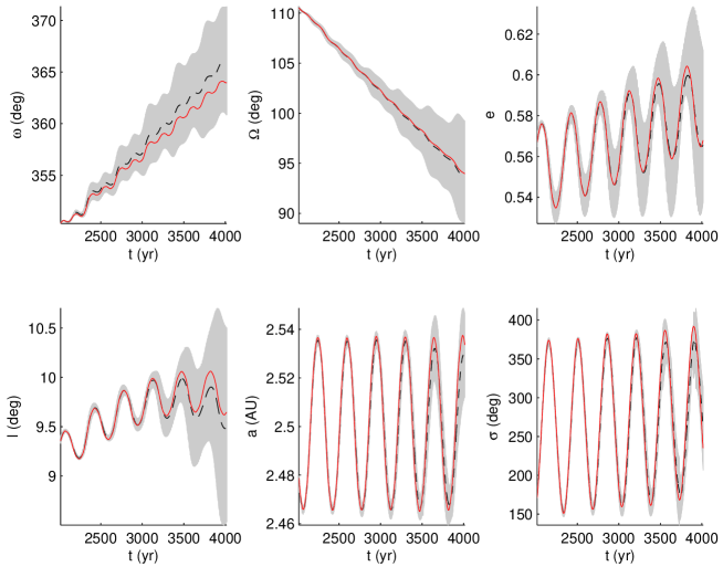
Figure 3: Asteroid 887 (Alinda): comparison between the long term evolution using $n_{\rm max}=3$ (solid line) and the arithmetic mean of 64 full numerical integrations (dashed line).

For asteroid 1685a we proceed in the same way, with the Earth playing the role of Jupiter. For the long term evolution we used $n_{\rm max}=3,15$. In Figure 4 we show the results. Using $n_{\rm max}=15$ we see that the result improves very much. The Earth crossing singularity occurs around $t=2281\>yr$. In this test the value of $\sigma_{c}$ at crossing results to be about $348$ degrees, which is quite different from all the values of $\sigma$ in Figure 4. We cannot really appreciate the effect of the singularity in the evolution since we obtain very small values of the components $\mathrm{Diff}_{h}(\frac{\partial\mathscr{H}}{\partial y_{i}})$.

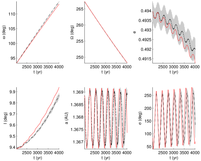
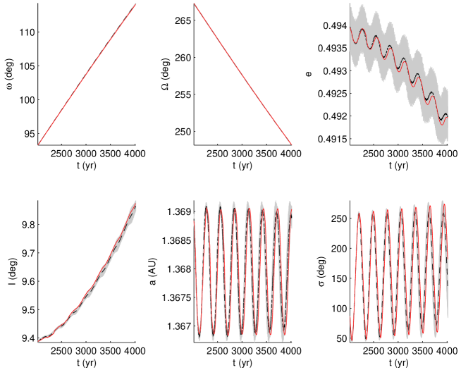
Figure 4: Asteroid 1685a: comparison between the long term evolution (solid line) and the arithmetic mean of 64 full numerical integrations (dashed line). Above $n_{\rm max}=3$. Below $n_{\rm max}=15$.

8 Conclusions

We studied the long term dynamics of an asteroid under the gravitational influence of the Sun and the solar system planets, assuming that a mean motion resonance between the asteroid and one of the planets occurs. We focused on the case of planet crossing asteroids and considered a resonant normal form $\mathscr{H}_{n_{\rm max}}$, see (7),(8). The analysis is performed separately for crossings with the resonant planet or with another one. In both cases, we could define generalized solutions of the differential equations for the long term dynamics, going beyond the singularity. These solutions are continuous but in general not differentiable. We also proved that generically, in a neighborhood of a crossing time, the evolution of the signed orbit distance along the generalized solutions is more regular that the long term evolution of the orbital elements. In case of crossings with the resonant planet, we recovered the protection mechanism against collisions in the limit $n_{\rm max}\to\infty$. This implies that, if the resonant angle $\sigma$ is different from the critical value $\sigma_{c}$ at the crossing times $t_{c}$ (see Sections 5,6) also deep close encounters are avoided, which makes the results of this theory more reliable. Indeed, close encounters can still occur with a planet not involved in the resonance, and this represent a critical case. Actually, in this case the semimajor axis usually suffer a drastic change [12], pushing the asteroid outside the considered resonance. By means of numerical experiments, in some relevant cases, we showed that the model seems to approximate well the full evolution in a statistical sense. We plan to make numerical tests on a large scale, to study different dynamical behaviors of the population of NEAs.

This work extends the results in [7] to the resonant case and gives a unified view of the orbit crossing singularity in case of mean motions resonances with one planet: indeed, comparing the results in Corollaries 1,2 we see how the discontinuity in the derivatives, represented by $\mathrm{Diff}_{h}\frac{\partial\mathscr{H}}{\partial y_{i}}$, vanishes in a weak sense (i.e. in the sense of distributions) for $n_{\rm max}\to\infty$, if $\sigma\neq\sigma_{c}$. Moreover, the resonant normal form introduced in (8) can easily be extended to include more than one resonance, also with different planets, by considering all the harmonics associated to the corresponding resonant module (see [11, Chap.2]).

Appendix A Appendix

From the definition of the approximate distance $\delta_{h}$, we have that

$$d^{2}(\mathcal{E},V)=d^{2}_{h}(\mathcal{E})+(V-V_{h})\cdot\mathcal{A}_{h}(V-V_{h})+{\cal R}_{3}^{(h)}(\mathcal{E},V)=\delta_{h}^{2}(\mathcal{E})+{\cal R}_{3}^{(h)}(\mathcal{E},V).$$

We summarize below some relevant estimates and results from [7]. In the following, we shall denote by $c_{i}$, $i=1,\dots,14$, some positive constants independent on $\mathcal{E}$. We first recall some Lemmas.

Lemma 1.

There exist positive constants $c_{1}$, $c_{2}$ and a neighborhood ${\cal U}$ of $(\mathcal{E}_{c},V_{h}(\mathcal{E}_{c}))$ such that

$$c_{1}\delta_{h}^{2}\leq d^{2}\leq c_{2}\delta_{h}^{2}$$

holds for $(\cal E,V)$ in ${\cal U}$. Moreover, there exist positive constants $c_{3}$, $c_{4}$ and a neighborhood ${\cal W}$ of $\mathcal{E}_{c}$ such that

$$d_{h}^{2}+c_{3}|V-V_{h}|^{2}\leq\delta_{h}^{2}\leq d_{h}^{2}+c_{4}|V-V_{h}|^{2}$$ (26)

holds for $\mathcal{E}$ in ${\cal W}$ and for every $V\in\mathbb{T}^{2}$.

Lemma 2.

Using the coordinate change $\xi={\cal A}_{h}^{1/2}(V-V_{h})$ and then polar coordinates $(\rho,\theta)$, defined by $(\rho\cos\theta,\rho\sin\theta)=\xi$, we have

$$\int_{{\cal D}}\frac{1}{\delta_{h}}\,d\ell d\ell^{\prime}=\frac{1}{\sqrt{\det{\cal A}_{h}}}\int_{{\cal B}}\frac{1}{\sqrt{d_{h}^{2}+|\xi|^{2}}}\,d\xi=\frac{2\pi}{\sqrt{\det{\cal A}_{h}}}(\sqrt{d_{h}^{2}+r^{2}}-d_{h})\,,$$ (27)

with ${\cal B}=\{\xi\in\mathbb{R}^{2}:|\xi|\leq r\}$. The term $-2\pi d_{h}/\sqrt{\det{\cal A}_{h}}$ is not differentiable at ${\cal E}={\cal E}_{c}\in\Sigma$.

Lemma 3.

The maps

$$\mathcal{W}^{+}\ni\mathcal{E}\mapsto\frac{\partial}{\partial y_{i}}\int_{\mathbb{T}^{2}}\frac{1}{\delta_{h}(\mathcal{E},V)}dV,\quad\mathcal{W}^{-}\ni\mathcal{E}\mapsto\frac{\partial}{\partial y_{i}}\int_{\mathbb{T}^{2}}\frac{1}{\delta_{h}(\mathcal{E},V)}dV$$

can be extended to two different analytic maps $\mathcal{G}_{h}^{+}$, $\mathcal{G}_{h}^{-}$ such that, in $\mathcal{W}$,

$$\mathcal{G}_{h}^{-}-\mathcal{G}_{h}^{+}=4\pi\biggl{[}\frac{\partial}{\partial y_{i}}\biggl{(}\frac{1}{\sqrt{\det(\mathcal{A}_{h})}}\biggr{)}\tilde{d}_{h}+\frac{1}{\sqrt{\det(\mathcal{A}_{h})}}\frac{\partial\tilde{d}_{h}}{\partial y_{i}}\biggr{]}.$$

Moreover the following estimates hold, with $\mathcal{U}_{\Sigma}=\{(\mathcal{E},V_{h}(\mathcal{E})):\mathcal{E}\in\Sigma\}$:

• $$\int_{\mathcal{D}}\frac{\partial^{2}}{\partial y_{i}\partial y_{j}}\frac{1}{d(\mathcal{E},V)}dV\leq c_{5}\quad\mbox{for }{\cal E}\mbox{ in }{\cal W},$$ (28)

• $$\left|\frac{\partial d^{2}}{\partial y_{i}}\right|,\left|\frac{\partial\delta_{h}^{2}}{\partial y_{j}}\right|\leq c_{6}(d_{h}+|V-V_{h}|)\quad\mbox{in }{\cal U}\setminus{\cal U}_{\Sigma},$$ (29)

• $$\int_{\cal D}\frac{dV}{d_{h}+|V-V_{h}|}\leq c_{7}\quad\mbox{for }{\cal E}\mbox{ in }{\cal W},$$ (30)

• $$\left|\frac{\partial^{2}\delta_{h}^{2}}{\partial y_{i}\partial y_{j}}\right|,\left|\frac{\partial^{2}d^{2}}{\partial y_{i}\partial y_{j}}\right|\leq c_{8}\quad\mbox{for }{\cal E}\mbox{ in }{\cal W},$$ (31)

• $$\left|\frac{1}{d^{3}}-\frac{1}{\delta_{h}^{3}}\right|\leq\frac{c_{9}}{d_{h}^{2}+|V-V_{h}|^{2}}\quad\mbox{in }{\cal U}\setminus{\cal U}_{\Sigma},$$ (32)

• $$\frac{\partial{\cal R}_{3}^{(h)}}{\partial y_{i}}\leq c_{10}|V-V_{h}|^{2}\quad\mbox{in }{\cal U}\setminus{\cal U}_{\Sigma},$$ (33)

• $$\frac{\partial^{2}{\cal R}_{3}^{(h)}}{\partial y_{i}\partial y_{j}}\leq c_{11}|V-V_{h}|\quad\mbox{in }{\cal U}\setminus{\cal U}_{\Sigma},$$ (34)

• $$\left|\frac{1}{d}-\frac{1}{\delta_{h}}\right|\leq{c_{12}}\quad\mbox{in }{\cal U}\setminus{\cal U}_{\Sigma},$$ (35)

• $$\left|\frac{\partial}{\partial y_{i}}\left(\frac{1}{d}-\frac{1}{\delta_{h}}\right)\right|\leq\frac{c_{13}}{d_{h}+|V-V_{h}|}\quad\mbox{in }{\cal U}\setminus{\cal U}_{\Sigma},$$ (36)

• $$\frac{\partial V_{h}}{\partial y_{i}}\leq c_{14}\quad\mbox{for }{\cal E}\mbox{ in }{\cal W}.$$ (37)

Acknowledgments. We are grateful to Alessandro Morbidelli, whose comments induced us to investigate better the relation between this work and the other results present in the literature, as explained in Section 6. The authors acknowledge the support by the Marie Curie Initial Training Network Stardust, FP7-PEOPLE-2012-ITN, Grant Agreement 317185. S.M. also acknowledges financial support from the Spanish Ministry of Economy and Competitiveness, through the ”Severo Ochoa” Programme for Centres of Excellence in R&D (SEV-2015-0554), the project ”Geometric and numerical analysis of dynamical systems and applications to mathematical physics” (MTM2016-76072-P), and the ”Juan de la Cierva-Formación” Programme (FJCI-2015-24917). G.F.G. has been partially supported by the University of Pisa via grant PRA-2017 ‘Sistemi dinamici in analisi, geometria, logica e meccanica celeste’.

References

[1] Arnold, V.I, Kozlov, V.V., Neishtadt, A.I.: Mathematical Aspects of Classical and Celestial Mechanics ,
Springer, 1997
[2] Dieudonné, J.: Foundations of Modern Analysis,
Academic press, 1969
[3] Gronchi, G.F.: Theoretical and computational aspects of
collision singularities in the -body problem, PhD thesis,
Univ. of Pisa (2002)
[4] Gronchi, G.F.: Generalized averaging principle
and the secular evolution of planet crossing orbits,
Cel. Mech. Dyn. Ast. 83 (2002), 97-120
[6] Gronchi, G.F., Tommei, G.: On the uncertainty of
the minimal distance between two confocal Keplerian orbits,
Discrete Contin. Dyn. Syst. Ser. B 7 (2007), 755-778
[7] Gronchi, G.F., Tardioli, C: Secular evolution of
the orbit distance in the double averaged restricted three-body
problem with crossing singularities, Discrete
Contin. Dyn. Syst. Ser. B 18 (2013), 1323-1344
[8] Lidov, M.L., Ziglin, S.L.: The Analysis of
Restricted Circular Twice-averaged Three Body Problem in the Case of
Close Orbits, Cel. Mech. 9/2 (1974), 151-173
[9] Milani, A., Baccili, S.: Dynamics of
Earth-crossing asteroids: the protected Toro orbits,
Cel. Mech. Dyn. Ast. 71/1 (1998), 35-53
[10] Milani, A., Carpino, M., Hahn, G., Nobili, A.M.:
Dynamics of Planet Crossing Asteroids: Classes of Orbital
Behavior, Icarus 78 (1989), 212-269
[11] Morbidelli, A.: Modern Celestial Mechanics
Taylor & Francis, 2002
[12] Valsecchi, G.B., Milani, A., Gronchi, G.F., Chesley, S.R.: Resonant returns to close approaches: Analytical theory
Astron. Astrophys. 408 (2003), 1179-1196
[13] Stein, E.M. and Shakarchi, R.: Fourier
Analysis. An introduction in Princeton Lectures in Analysis
I. Princeton University Press, 2003
[14] Whipple, A.: Lyapunov times of the inner
asteroids, Icarus 115 (1995), 347-353
[15] Wisdom, J.: Chaotic behavior and the origin of
the 3/1 Kirkwood gap, Icarus 56 (1983), 51-74