Interplay of interfacial noise and curvature driven dynamics in two dimensions

Abstract

We explore the effect of interplay of interfacial noise and curvature driven dynamics in a binary spin system. An appropriate model is the generalised two dimensional voter model proposed earlier (J. Phys. A: Math. Gen. 26, 2317 (1993)), where the flipping probability of a spin depends on the state of its neighbours and is given in terms of two parameters $x$ and $y$. $x=0.5,y=1$ corresponds to the conventional voter model which is purely interfacial noise driven while $x=1$ and $y=1$ corresponds to the Ising model, where coarsening is fully curvature driven. The coarsening phenomena for $0.5<x<1$ keeping $y=1$ is studied in detail. The dynamical behaviour of the relevant quantities show characteristic differences from both $x=0.5$ and $1$. The most remarkable result is the existence of two time scales for $x\geq x_{c}$ where $x_{c}\approx 0.7$. On the other hand, we have studied the exit probability which shows Ising like behaviour with an universal exponent for any value of $x>0.5$; the effect of $x$ appears in altering the value of the parameter occurring in the scaling function only.

Nonequilibrium phenomena associated with the zero temperature ordering process in classical Ising and Voter models liggett ; krapbook ; castellano ; socio have been extensively studied in the recent past. Both models are two state models and the states can be represented by Ising spins. There is, however a basic difference. The Ising model (IM) is defined using an energy function ($H=-J\sum\sigma_{i}\sigma_{j}$; where $\sigma=\pm 1$ and the sum is usually over nearest neighbours) and it has no intrinsic dynamics. However, starting from a configuration far from equilibrium, one can study the time dependent behaviour of the so called kinetic Ising model. At zero temperature, the time evolution essentially corresponds to an energy minimising scheme Glauber in the standard rules like single spin flip Glauber or Metropolis dynamics. The Voter model (VM) on the other hand has no such energy function associated - it is defined by the dynamical rule that an agent follows the state of a randomly chosen neighbour at each time step. The kinetic Ising and Voter models are known to be identical in one dimension while in higher dimensions the dynamical schemes are markedly different dornic . While the coarsening is curvature driven in the Ising model, it is interfacial noise driven in the Voter model. This results in different behaviour of the relevant dynamical variables like density of active bonds $n(t)$, persistence probability $P(t)$ and time scales. Active bonds are those which connect neighbouring spins with opposite signs. In one dimension, for both the Ising and Voter models, $n(t)$ shows power law decay as $t^{-\frac{1}{2}}$. This behaviour is true for the Ising model even in higher dimensions. But for the Voter model, $n(t)$ asymptotically vanishes as $\frac{1}{\ln t}$ in two dimensions and for dimensions $d>2$, $n(t)\sim a-bt^{-d/2}$. The dynamics in VM is slower and the consensus time (by consensus we mean the all up and all down absorbing states of the system) typically behaves as $L^{2}\log L$ in contrast to $L^{2}$ for the IM in two dimensions ($L$ is the system size). The persistence probability $P(t)$, defined as the probability that a spin does not change sign till time $t$, shows algebraic decay as $t^{-\theta}$ with $\theta=0.375$ in one dimension Derrida1 ; Derrida2 ; Derrida3 ; satya for the two models. For the the IM, $P(t)$ shows algebraic decay even in higher dimensions; in two dimensions $\theta\approx 0.2$ bray ; yurke ; sire ; picco . However, for the two dimensional VM, $P(t)$ has the behaviour $\exp[-$constant$(\ln t)^{2}]$ ben . The spin autocorrelation function is another dynamical quantity which again shows different behaviour for the VM and the IM in two dimensions ben ; auto1 ; auto2 ; auto3 ; auto4 .

Another interesting feature of the $Z_{2}$ models (models with spin up and spin down symmetry) with two absorbing states (which are either all spins up or down) is the exit probability $E(\rho)$. $E(\rho)$ is defined as the probability that the final state has all up spins starting with a density $\rho$ of up spins. The exit probability $E(\rho)$ is also different in the two models for $d>1$. It can be easily argued that in all dimensions, $E(\rho)=\rho$ for the VM. With only nearest neighbour interaction, $E(\rho)$ is obviously linear for the IM also in one dimension. However, allowing further neighbour interactions and other parameters governing the dynamics, a nonlinear behaviour can be observed even in one dimension for both Ising model and Voter model pr ; lamred1 ; lamred2 . This implies that there is a scope for phenomena like “minority spreading” minor always in one dimension. In the two dimensional Ising model $E(\rho)$ shows non-linear behaviour Pm which in the thermodynamic limit approaches a step function. It may be mentioned here that in the zero temperature ordering of Ising model, one encounters the problem of frozen states redner ; spirin . Hence, the calculation of exit probability is made using only those configurations which reach the all up or all down states.

Since the interfacial noise and surface tension governed dynamics definitely lead to highly different dynamical behaviour of several important quantities, it is worthwhile to study models in which both are present in a tunable manner. One such model had been proposed in oliveira , namely the generalised voter model. We have, therefore, considered this particular model to study the interplay of the interfacial noise and curvature driven dynamics.

In the generalised voter model, the dynamical rule has been parameterised so that one can recover a number of models for specific values of the parameters. We have investigated the behaviour of the persistence probability, decay of active bonds, exit probability and time to reach consensus. These quantities are not related in general and hence the effect of changing the parameter values may be different for each of them.

Let us briefly review the generalised Voter model (GVM henceforth) proposed in oliveira . Here, at each site of the square lattice there is a spin variable $\sigma_{i}=\pm 1$. The configuration evolves in time according to single spin flip stochastic dynamics. The spin flip probability $w_{i}(\sigma)$ for the $i$th spin is given by,

$$w_{i}(\sigma)=\frac{1}{2}[1-\sigma_{i}f_{i}(\sigma)],$$ (1)

where $f_{i}(\sigma)=f(\sum_{\delta}\sigma_{i+\delta})$, a function of the sum of the nearest neighbor spin variables. The model is defined taking $f(0)=0$, $f(2)=-f(-2)=x$ and $f(4)=-f(-4)=y$, where $x$ and $y$ are restricted to the conditions $x\leq 1$ and $y\leq 1$. The original VM is recovered for $x=0.5$ and $y=1$ whereas the IM corresponds to $x=1,y=1$. Along the line $y=1$, there are two absorbing states: all spins up and all spins down for $x\geq 0.5$ (apart from possible frozen states). These states are however unstable for $x<0.5$. As the limiting values $x=0.5$ and $x=1.0$ correspond to the two different models, one can expect either a sharp transition or a crossover behaviour at an intermediate value of $x$.

We have studied the non-equilibrium behaviour and exit probability $E(\rho)$ of the GVM keeping $y=1$ and varying $x$ using Monte Carlo simulations on $L\times L$ square lattices with $L\leq 80$. Periodic boundary conditions have been used and at least $2500$ different initial configurations have been simulated. Persistence probability, active bonds dynamics and consensus times are the quantities estimated. These quantities are unrelated and therefore it is useful to study all of these to check how each of them is effected by tuning of the parameter $x$.

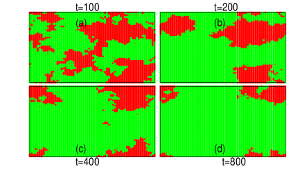
Figure 1: Typical snapshots at different times for $x=0.6$ shows that coarsening is curvature driven.

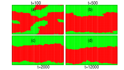
Figure 2: Certain configurations show very slow relaxation as $x$ is increased. Snapshots show such a configuration for different times for $x=0.9$.

Snapshots taken during the evolution help in understanding the process quite well. We find that in general for $x>0.5$ , the pictures looks very similar to the curvature driven case. However for $x$ close to $1$, certain configurations show the existence of nearly striped patterns which do reach consensus but very slowly as the interfaces take long time to vanish. In Figs 1 and 2, we have shown snapshots for two values of $x$; for $x=0.6$, the curvature driven coarsening is seen to dominate while for $x=0.9$, a case is shown where coarsening has led to domains with nearly straight edges prevailing over large time durations. Snapshots for other values of $x$ are given in the SM .

The variation of the density of active bonds $n(t)$ against time is plotted in Fig. 3 for different values of $x$. As $x$ increases from $0.5$, we find that $n(t)$ goes to zero involving larger time scales. However, the variation is faster than the $1/\log t$ behaviour known for the Voter model. It is found that for any $0.5\leq x<1$ the system always reaches the equilibrium ground state since $n(t)$ vanishes which implies the freezing probability is zero. Only at $x=1$ a frozen state may be reached. As $x$ approaches unity (but not equal to it), the initial decay of $n(t)$ can be fitted quite accurately by a power law, while there is a clear crossover to a much slower evolution at later times as shown in the inset of Fig. 3. This suggests that there are two different time regimes. There is an initial time scale up to which the behaviour is similar to the Ising model, i.e., $n(t)$ shows a power law decay with exponent close to 1/2. Beyond this scale, a non algebraic slow decay is observed. However, we have checked that the behaviour in the later regime is not like $1/\log t$ as in the Voter model but may be even slower than that. For general values of $x$, we conjecture that at initial times a power law behaviour occurs with some correction to scaling as indicated by the plots in Fig. 3; such corrections become weaker as $x$ deviates from 0.5. The second regime with the slower decay exists only for $x>x_{c}$, $x_{c}\approx 0.7$. For exactly $x=1$, the power law behaviour is exact before $n(t)$ saturates to a time independent non-zero value due to the frozen stable states.

In order to gain more insight in the dynamical behaviour, we have estimated the time $\tau$ required to reach the consensus state and its distribution $D(\tau)$. In a detailed study made for $L=32$, we find that $D(\tau)$ changes its nature remarkably as $x$ is increased (Fig. 4). For $x=0.5$, $D(\tau)$ shows a conventional behaviour; it increases for small $\tau$, has a broad peak and a long exponential tail. This behaviour continues till $x_{c}\approx 0.70$ beyond which we find that $D(\tau)$ differs considerably for small and large values of $\tau$ (see Fig, 8 in SM). Apparently it is an overlap of a symmetric function of finite width peaked about a small value of $\tau$ and a slow exponentially decaying function extending to large values of $\tau$ (a magnified figure is shown in Fig. 7 in the SM). Exactly at $x=1$, the width of the symmetric function is minimum and the exponential part exists over a much shorter range. We conjecture that in the thermodynamic limit, the exponential part of $D(\tau)$ for $x=1$ will vanish altogether; this is supported by the data for $L=64$ (shown in SM ). As the tail of the distribution for any $x$ may be fit by an exponential function $\exp(-\omega\tau)$ one can define a time scale $\tau_{eff}=1/\omega$ for each $x$.

In Fig 5, we plot the three time scales: $\tau_{eff}$, $\langle\tau\rangle$ and $\tau_{mp}$ where $\tau_{mp}$ denotes the most probable value. In general, the average values of $\tau$ are different from the most probable values. The difference becomes considerable for $x>x_{c}$ due to the long exponential tails. From Fig. 5 we can conclude that $\tau_{mp}$ is very weakly dependent on $x$; in fact for $x\geq 0.55$, it is almost a constant. On the other hand the two other timescales are strongly dependent on $x$; $\tau_{eff}$ and $\langle\tau\rangle$ initially decrease and then increase rapidly with $x$. Evidently, $\tau_{mp}$ denotes the time to reach consensus in absence of any intermediate metastable state and is presumably constant for any $x>0.5$. On the other hand, $\tau_{eff}$ corresponds to the time scale associated with the configurations with nearly frozen intermediate states which increase in number as $x$ increases. $\langle\tau\rangle$ shows the increasing trend simply because it is an overall average.

The existence of the two different time scales is clearly shown by the above result. The non-monotonicity in $\langle\tau\rangle$ and $\tau_{eff}$ are to be noted, both time scales drop immediately as $x$ deviates from 0.5 and again at $x=1$. This suggests there are discontinuities at the two well known limiting points.

The average consensus times as a function of the different system sizes apparently show a behaviour faster than $L^{2}\log L$ for $x>0.5$. $\langle\tau\rangle$ for other values of $L$ are shown in the SM . The possibility of discontinuities existing at $x=0.5$ and $x=1$ is more strongly supported by the data as system size increases. A more conclusive statement about the scaling of the timescales with the system sizes can only be made after a detailed study of the other time scales which is to be reported later.

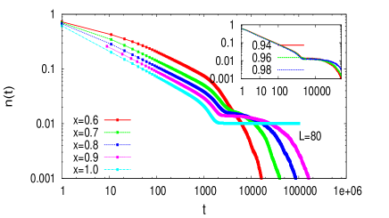
Figure 3: Plot of density of active bonds with time $t$ for $L=80$ for $x=0.6,0.7,0.8,0.9,1$. Inset shows variation of active bonds for $x=0.94,0.96,0.98$.

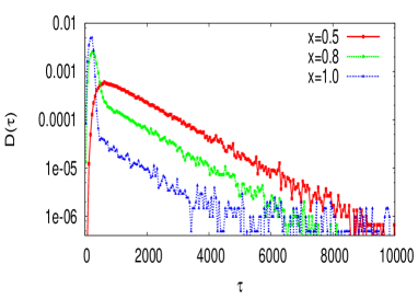
Figure 4: Plot of distribution of consensus time for $x=0.5,0.8,1$.

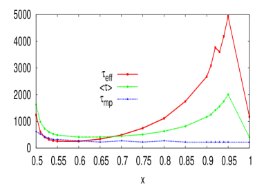
Figure 5: Plot of different time scales $\tau_{eff}$, $\langle\tau\rangle$ and $\tau_{mp}$ as a function of $x$.

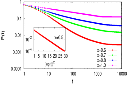
Figure 6: Plot of persistence probability with time $t$ for $L=80$ for $x=0.6,0.7,0.8,1$. Inset shows variation of $P(t)$ as a function of $(\ln t)^{2}$ for $x=0.5$.

We next discuss some other results in context of the nonequilibrium phenomena. The persistence probability $P(t)$ as a function of time $t$ is plotted in Fig. 6. For $x=1$, $P(t)$ shows power law decay as $t^{-\theta}$ with $\theta\simeq 0.2$ agreeing with the known result bray ; yurke ; sire ; picco . For $x=0.5$, persistence decays to a very small fraction ($\approx 0$) following the behaviour $\exp[-0.31(\ln t)^{2}]$. This behaviour is obtained by fitting the data and agrees very well with the form obtained numerically in ben . For $0.5<x<1$, $P(t)$ also approaches a non-zero saturation value, however there is no clear power law behaviour. The saturation value increases with increase in $x$ in a non-linear manner.

Lastly we discuss the results for the exit probability (see Fig. 7). The plot of $E(\rho)$ as a function of $\rho$ shows that it is nonlinear except for $x=0.5$ having strong system size dependence. Different curves intersect at a single point $\rho=\rho_{c}\simeq 0.5$ ($\rho_{c}$ should be equal to 0.5 from symmetry argument). The curve becomes steeper as the system size is increased. Finite size scaling analysis as in sbiswas can be made using the scaling form

$$E(\rho,L)=f\left[\frac{(\rho-\rho_{c})}{\rho_{c}}L^{1/\nu}\right],$$ (2)

where $f(y)\to 0$ for $y<<0$ and equal to $1$ for $y>>0,$ so that the data for different system sizes $L$ collapse when $E(\rho)$ is plotted against $\frac{(\rho-\rho_{c})}{\rho_{c}}L^{1/\nu}$. The data collapse takes place with $\nu=1.3~{}\pm~{}0.01$ (the unscaled data is shown in the bottom inset) for all values of $x>0.5$. We conclude that like the Ising model, $E(\rho)$ becomes a step function in the thermodynamic limit. The scaling form given by eq. (2) is found to fit very well with a general form sbiswas

$$f(y)=\frac{1+\tanh(\lambda y)}{2},$$ (3)

where $\lambda$ depends on $x$. The dependence of $\lambda$ on $x$ is shown in the top left inset of Fig. 7. $\lambda$ which increases with $x$ quantifies the steepness of the $E(\rho)$ curve. $\lambda$ increases continuously as $x$ is increased from $0.5$, consistent with the fact that the $E(\rho)$ should deviate from the linear behaviour. However, exactly at $x=1$, $\lambda$ increases abruptly to a comparatively larger value indicating a discontinuity.

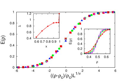
Figure 7: Data collapse of $E(\rho)$ is plotted against $\frac{(\rho-\rho_{c})}{\rho_{c}}L^{1/\nu}$ for system sizes $L=32,48,64,80$ for $x=0.6$. Bottom inset shows plot of unscaled data against $\rho$. Top inset shows the plot of $\lambda$ as a function of $x$.

Let us now discuss the results obtained in this Rapid Communication. First of all it appears that the curvature driven coarsening governs the dynamics for any $x>0.5$ at least in the initial stages. This is evident from Fig. 3, which shows that at initial times the ordering becomes much faster compared to the Voter model as $x$ is increased from $0.5$ (see Fig. 5 in SM ). At the same time, the interfacial noise driven coarsening present in the system, however small, is crucial for leading the system to consensus for larger values of $x$ when the dominant curvature driven process tends to generate nearly straight interfaces. It is only because of its presence the freezing probability is zero in the system for any $x\geq 0.5$ (but not equal to unity). Thus it is interesting to note that while for smaller values of $x$ the model is closer to the voter model, the average consensus time increases as $x$ approaches unity, the Ising limit. This is apparently counter intuitive as it is known that the evolution in the Voter model is slower compared to that in the Ising model in two dimensions. Actually the metastable states increase in number as $x$ is increased (which is not surprising knowing the result for $x=1$) enabling longer time scales for the system. However average consensus times are still less than that at $x=0.5$ up to a certain value of $x$. Results for different system sizes indicate that this value is very close to $x_{c}$ (shown in SM ) in the thermodynamic limit which is consistent with the other results.

The exit probability shows a nonlinear behaviour for any $x>0.5$ with a universal exponent $\nu~{}\approx 1.3$ and a non-universal parameter $\lambda$ entering the scaling function. Since we omit the frozen states for $x=1$ and the time scales are irrelevant for this measure, it is not surprising that the behaviour is Ising like. However, the fact that $\lambda$ shows a discontinuity at $x=1$ again shows that the $x=1$ point has a distinctive feature with respect to the exit probability as well.

In conclusion, quite a few interesting results due to the interplay of the two types of dynamics are obtained in the genaralised Voter model. The main result is the existence of two time scales in the system for $x>x_{c}$.One of them, $\tau_{mp}$ is nearly independent of $x$ while $\tau_{eff}$, the other timescale is a highly nonlinear function of $x$. Both $x=0.5$ and $x=1$ with completely different kind of dynamical rules have unique features. At $x=0.5$, $P(t)$ and $E(\rho)$ behave differently compared to any other value of $x>0.5$, $\langle\tau\rangle$ is discontinuous. On the other hand, $x=1$ is also unique in the sense freezing occurs only at this point, $\langle\tau\rangle$ and $\lambda$ show discontinuity here while well known power law behaviour in the relevant quantities exist. The intermediate region $0.5<x<1$ does not show any freezing phenomena. Although not algebraic, here $P(t)$ reaches saturation for $0.5<x<1$ in contrast to that at $x=0.5$. No sharp transition is observed for any value of $0.5<x<1$, but a crossover behaviour at $x=x_{c}\approx 0.7$ is seen to exist.

Acknowledgement: PR acknowledges financial support from UGC. PS acknowledges financial support from CSIR project.

References

- (1) T. M. Liggett, Interacting Particle Systems, Springer, New York (1985).
- (2) P. L. Krapivsky, S. Redner, E. Ben-Naim, A Kinetic View of Statistical Physics, Cambridge University Press, Cambridge (2010).
- (3) C. Castellano, S. Fortunato and V. Loreto, Rev. Mod. Phys. 81, 591 (2009).
- (4) P. Sen and B. K. Chakrabarti, Sociophysics: An Introduction, Oxford University Press, Oxford (2013).
- (5) R. J. Glauber, J. Math. Phys. 4, 294 (1963).
- (6) I. Dornic, H. Chaté, J. Chave, and H. Hinrichsen,Phys. Rev.Lett.87, 045701 (2001).
- (7) B. Derrida, A. Bray and C. Godreche, J. Phys. A: Math. Gen. 27, L357 (1994).
- (8) B. Derrida, J. Phys. A: Math. Gen. 28, 1481 (1995).
- (9) B. Derrida, V. Hakim and V. Pasquier, Phys. Rev. Lett. 75, 751 (1995).
- (10) S. N. Majumdar, Current Science, 77, 370 (1999).
- (11) A. J. Bray, S. N. Majumdar and G. Schehr, Adv. Phys. 62, 225 (2013).
- (12) B. Yurke, A. N. Pargellis, S. N. Majumdar and C. Sire, Phys. Rev. E 56, R40 (1997).
- (13) S. N. Majumdar and C. Sire, Phys. Rev. Lett. 77, 1420 (1996).
- (14) T. Blanchard, L. F. Cugliandolo and M. Picco, J. Stat. Mech. 2014 12021 (2014).
- (15) E. Ben-Naim, L. Frachebourg, and P. L. Krapivsky, Phys. Rev. E 53, 3078, (1996).
- (16) D. A. Huse and D. S. Fisher, Phys. Rev. B35,6841 (1987).
- (17) H. Takano, H. Nakanishi and S. Miyashita, Phys. Rev. B 37, 3716 (1988).
- (18) C. Tang, H. Nakanishi and J. S. Langer, Phys. Rev. A 40, 995 (1989).
- (19) L. Golubović and S. Feng, Phys. Rev. B 43, 972 (1991).
- (20) P. Roy and P. Sen, Phys. Rev. E 89, 030103 (R), (2014).
- (21) R. Lambiotte and S. Redner, J. Stat. Mech. 2007 L10001 (2007).
- (22) R. Lambiotte and S. Redner, Euro. Phys. Lett. 82, 18007 (2008).
- (23) S. Galam, Eur. Phys. J. B 25, 403, (2002).
- (24) P. Mallik and P. Sen, Phys. Rev. E 93, 052113, (2016).
- (25) V. Spirin, P. L. Krapivsky and S., Phys. Rev. E, 63, 036118 (2001).
- (26) V. Spirin, P. L. Krapivsky and S., Phys. Rev. E, 65, 016119 (2001).
- (27) M. J. de Oliveira, J. F. F. Mendes and M. A. Santos, J. Phys. A: Math. Gen. 26, 2317 (1993).
- (28) See Supplemental Material at [URL will be inserted by publisher] for [snapshots and other figures and results for ].
- (29) S. Biswas, S. Sinha and P. Sen, Phys. Rev. E 88, 022152 (2013).