Frequency regularities of acoustic modes and multi-colour mode identification in rapidly rotating stars

Abstract

Context. Mode identification has remained a major obstacle in the interpretation of pulsation spectra in rapidly rotating stars. This has motivated recent work on calculating realistic multi-colour mode visibilities in such stars.

Aims. We would like to test mode identification methods and seismic diagnostics in rapidly rotating stars, using oscillation spectra based on these new theoretical predictions.

Methods. We investigate the auto-correlation function and Fourier transform of theoretically calculated frequency spectra, in which modes are selected according to their visibilities. Given that intrinsic mode amplitudes are determined by non-linear saturation and cannot currently be theoretically predicted, we experimented with various ad-hoc prescriptions for setting the mode amplitudes, including using random values. Furthermore, we analyse the ratios between mode amplitudes observed in different photometric bands to see up to what extent they can identify modes.

Results. When non-random intrinsic mode amplitudes are used, our results show that it is possible to extract a mean value for the large frequency separation or half its value, and sometimes twice the rotation rate, from the auto-correlation of the frequency spectra. Furthermore, the Fourier transforms are mostly sensitive to the large frequency separation or half its value. The combination of the two methods may therefore measure and distinguish the two types of separations. When the intrinsic mode amplitudes include random factors, as seems more representative of real stars, the results are far less favourable. It is only when the large separation or half its value coincides with twice the rotation rate, that it might be possible to detect the signature of a frequency regularity. We also find that amplitude ratios is a good way of grouping together modes with similar characteristics. By analysing the frequencies of these groups, it is possible to constrain mode identification as well as determine the large frequency separation and the rotation rate.

1 Introduction

One of the major obstacles in interpreting the acoustic frequency spectra of rapidly rotating stars is mode identification, i.e. finding the correspondence between theoretically calculated modes and observed pulsations. Several reasons make it difficult to match the two. First and foremost is the the lack of simple frequency patterns, such as what is present in solar-like stars. Indeed, rapid rotation leads to complex spectra with overlapping classes of pulsation modes, each with an independent frequency organisation (Lignières & Georgeot, 2008). Next comes the whole problem of mode amplitudes. Most rapid rotators tend to be massive or intermediate mass stars where modes are predominantly excited by the $\kappa$ mechanism. This leads to non-linear saturation and coupling between modes, making it nearly impossible to predict the amplitudes with current theory. Further difficulties include avoided crossings between modes, and all of the theoretical and numerical challenges associated with rapid rotation. From an observational point of view, the high quality data from space missions CoRoT (Baglin et al., 2009; Auvergne et al., 2009) and Kepler (Borucki et al., 2009) have painted a new picture of $\delta$ Scuti stars, through the detection of hundreds of pulsation modes (Poretti et al., 2009; Balona et al., 2012). In a similar way, the number of detected modes has also increased for stars from other classes of rapidly rotating pulsators, and along with it the complexity of the spectra (e.g. Uytterhoeven et al., 2011). Consequently, most asteroseismic analyses have focused on interpreting the general characteristics of these spectra rather than identifying individual modes.

Various strategies have been devised in order to identify modes. One can, for instance, search for frequency patterns appropriate for rapid rotation. The background for this search is the discovery of asymptotically uniform frequency spacings in the numerically computed spectra of uniformly rotating polytropic models (Lignières et al., 2006; Reese et al., 2008) and differentially rotating realistic SCF models (Reese et al., 2009a). These uniform spacings have also been modelled through asymptotic semi-analytical formulas (Pasek et al., 2012). In observed spectra, recurrent frequency spacings which may correspond to the large separation or half its value have been found in some stars (García Hernández et al., 2009, 2013; Paparó et al., 2016). Moreover, García Hernández et al. (2015) showed that mean density estimates based on such spacings (obtained via a scaling relation similar to the one in Reese et al., 2008, but based on SCF models) are compatible with independent mass and radii measurements obtained for $\delta$ Scuti stars in binary systems. Nonetheless, it is expected that various effects should contribute to hide these regular frequency patterns. First, as mentioned before, the full spectrum is a superposition of sub-spectra corresponding to different classes of modes and some of the uniform spacings only concern one class. This complicates their detection in the full spectrum. Also, due to their asymptotic nature, these spacings might not be relevant to analyse the low to moderate (up to radial order $n\sim 10$) frequency domain, typical of most rapidly rotating pulsators. A third effect that might come into play is the presence of mixed modes in evolved stars and/or sharp sound speed gradients as they can potentially modify the regular spacings. Finally, mode selection effects due to the non-linearly determined intrinsic mode amplitudes could affect the detectability of the regular patterns. As a first attempt, Reese et al. (2009b) developed a strategy to find these frequency spacings but ran into difficulties when including chaotic modes, which come from another class of modes. Lignières et al. (2010) addressed the same question with encouraging results but their analysis was restricted to the asymptotic regime and relied on simplifying assumptions regarding the spectrum of chaotic modes and the mode visibilities. In the present paper, our first goal is to search for regular frequency spacings in the most realistic synthetic spectra available, using relevant frequency ranges and accurate visibility calculations. While they can provide guidance to a similar search in real data, we already know that these results must be taken with caution since the intrinsic mode amplitudes used in the present paper are not realistic but based on ad-hoc prescriptions.

Another strategy which avoids this difficulty is to constrain the identification through multi-colour photometric or spectroscopic observations. Indeed, one can measure the amplitudes and the phases of a given pulsation mode in different photometric bands and then compare these by calculating amplitude ratios or phase differences. The geometry of the modes will then lead to different characteristic signatures. One important advantage of this method is that these signatures are independent of the intrinsic mode amplitude. In a similar fashion, the oscillatory movements induced by a pulsation mode cause Doppler shifts which show up as variations in the shape of spectroscopic absorption lines, known as “line profile variations” or LPVs. These variations are then directly related to the geometry of the mode. By comparing theoretical predictions with observations, one can then constrain the mode’s identification. In what follows, we will focus on multi-colour mode identification.

Most of the previous theoretical investigations of amplitude ratios and phase differences have been based on mode calculations which approximate the effects of rotation. For instance, Daszyńska-Daszkiewicz et al. (2002) used a perturbative approach, whereas Townsend (2003) and Daszynska-Daszkiewicz et al. (2007) applied the traditional approximation (which is typically used when calculating gravito-inertial modes). It is only recently that such predictions have started to fully take into account the effects of rotation. First, Lignières et al. (2006) and Lignières & Georgeot (2009) calculated disk-integration factors for pulsation modes calculated in fully deformed polytropic models. Given the simplified nature of these calculations, it was not possible to calculate associated amplitude ratios or phase differences. More recently, Reese et al. (2013b, hereafter Paper I) calculated mode visibilities in realistic models of rapidly rotating stars. This work relied on a grid of Kurucz atmospheres to calculate realistic emerging intensities, thereby taking into account limb and gravity darkening. It took into account the Lagrangian variations of temperature and effective gravity as well as the surface distortion from the pulsation modes. The pulsation modes were calculated using a 2D approach which takes into account centrifugal distortion. The main limitation was the adiabatic approximation which leads to an unreliable estimation of the Lagrangian variations of the effective temperature. Nonetheless, first results were obtained in that work which hopefully provide a qualitative insight, both into mode visibilities and multi-colour amplitude ratios.

In the following two sections, we succinctly recall some of the main aspects of pulsation modes in rapidly rotating stars, as well as the basic principles behind the visibility calculations described in Paper I. We then examine the auto-correlation functions of theoretically calculated spectra which overlap the p- and g-mode domains. This is followed by a discussion on Fourier transforms of frequency spectra and how these complement auto-correlation functions. In Section 6, we show how multi-colour photometric mode identification can be extended to rapidly rotating stars. Finally, a discussion concludes the paper.

2 Pulsation modes

Rapidly rotating models are calculated thanks to the Self-Consistent Field (SCF) method (Jackson et al., 2005; MacGregor et al., 2007). The resultant models represent ZAMS stars with a cylindrical rotation profile, and hence a barotropic stellar structure, i.e. a structure where different thermodynamic quantities such as the density, pressure, and temperature are constant on isopotential surfaces (deduced from the sum of the gravitational and centrifugal potentials). The pulsation modes are calculated using the Two-dimensional Oscillation Program (TOP Reese et al., 2006, 2009a). As described in Paper I, an improved treatment of the models and a slightly different mechanical boundary condition were necessary to obtain eigenfunctions appropriate for visibility calculations. Compared to Paper I, the frequency range has been extended both to higher and lower frequencies, including g-modes, although for the most part we focus on p-modes.

As was shown in Lignières & Georgeot (2008, 2009), acoustic modes subdivide into several classes of modes as the rotation rate increases. Each class of mode has its own typical geometry and frequency organisation, whether regular or statistical. This behaviour stems from the gradual transition of the ray dynamics system from being integrable to chaotic – a transition which causes different regions, associated with the different classes, to appear in the Poincaré section. Of particular interest are the island modes, the rotating counterpart to low degree modes. These modes focus around a periodic trajectory and are characterised by the quantum numbers $(\tilde{n},\,\tilde{\ell},\,m)$ where $\tilde{n}$ is the number of nodes along the trajectory, $\tilde{\ell}$ the number of nodes perpendicular to the trajectory, and $m$ the usual azimuthal order. As illustrated in the animation in Reese (2008), it is possible to transform these quantum numbers into the usual spherical quantum numbers $(n,\,\ell,\,m)$ and inversely, using the following relations based on what could be described as “node conservation”:

$$\left\{\begin{array}[]{rcl}\tilde{n}&=&2n+\varepsilon,\\ \tilde{\ell}&=&\frac{\ell-|m|-\varepsilon}{2},\\ \varepsilon&\equiv&(\ell+m)\,\,[2],\end{array}\right.\qquad\left\{\begin{array}[]{rcl}n&=&\frac{\tilde{n}-\varepsilon}{2},\\ \ell&=&2\tilde{\ell}+|m|+\varepsilon,\\ \varepsilon&\equiv&\tilde{n}\,\,[2],\end{array}\right.$$ (1)

where $\varepsilon$ corresponds to mode parity, i.e. $\varepsilon=0$ for even modes, modes which are symmetric with respect to the equator, and $\varepsilon=1$ for odd modes. One will note in particular that the parity of $\tilde{n}$ corresponds to that of the mode. This simply corresponds to the fact that the node along the equatorial plane is treated as a pseudo-radial node in island modes. Closely related to this is the fact that one set of $(\tilde{\ell},\,m)$ values corresponds to two sets of $(\ell,\,m)$ values depending on the parity of $\tilde{n}$, as illustrated in Fig. 1. At this point, it is also useful to introduce the large frequency separation, $\Delta$ and the semi-large frequency separation, $\Delta/2$:

$$\Delta = \omega_{n+1,\,\ell,\,m}-\omega_{n,\,\ell,\,m}=\omega_{\tilde{n}+2,\,\tilde{\ell},\,m}-\omega_{\tilde{n},\,\tilde{\ell},\,m},$$ (2)

$$\frac{\Delta}{2} = \omega_{\tilde{n}+1,\,\tilde{\ell},\,m}-\omega_{\tilde{n},\,\tilde{\ell},\,m},$$ (3)

where $\omega$ is the frequency, indexed either by the spherical or island mode quantum numbers.

Odd	Even
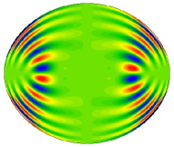
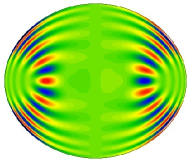
$(n,\,\ell,\,m)=(9,2,1)$	$(n,\,\ell,\,m)=(10,1,1)$
$(\tilde{n},\,\tilde{\ell},\,m)=(19,0,1)$	$(\tilde{n},\,\tilde{\ell},\,m)=(20,0,1)$

Figure 1: (colour online) Meridional cross-sections of two island modes with the same $(\tilde{\ell},\,m)$ values but opposing parity, as determined from the parity of $\tilde{n}$. The colours indicate the Eulerian pressure perturbation divided by the square root of the equilibrium density.

Recently, Pasek et al. (2012) found asymptotic expressions for the profile of island modes in the direction perpendicular to the periodic trajectory. Apart from a $1/\sqrt{\omega}$ scaling, modes with the same $(\tilde{\ell},\,m)$ values have the same transverse profile. This applies in particular at the stellar surface. Hence, modes with the same $(\tilde{\ell},\,m)$ values will have similar surface profiles in one hemisphere. They will be either symmetric or antisymmetric with respect to the equator depending on the parity of $\tilde{n}$. Note that using $\ell$ instead of $\tilde{\ell}$ also enables us to select island modes of the same equatorial parity. In addition, the weak influence of the Coriolis force on high-frequency acoustic modes (see Reese et al., 2006) implies that $\pm m$ pairs of mode are nearly identical (with near-degenerate frequencies in the corotating frame). It follows that island modes with the same $(\ell,\,|m|)$ values will have similar surface profiles. They should then have similar visibilities (as described in the next section) and this property will play an important role in the mode identification methods described in what follows.

3 Mode visibilities

Mode visibilities are obtained by perturbing the expression which gives the amount of energy radiated by a star to an observing instrument:

$$E=\frac{1}{2\pi d^{2}}\iint_{\mathrm{Vis.Surf.}}I(\mu,g_{\mathrm{eff}},T_{\mathrm{eff}})\@vec{e}_{\mathrm{obs.}}\cdot\@vec{\mathrm{d}S}$$ (4)

where $d$ is the distance to the star, $\mu$ the cosine of the angle between the outward normal to the stellar surface and the observer’s direction, “Vis. Surf.” the surface visible to the observer, $g_{\mathrm{eff}}$ and $T_{\mathrm{eff}}$ the effective gravity and temperature, and $I(\mu,g_{\mathrm{eff}},T_{\mathrm{eff}})$ the specific radiation intensity, multiplied by the instrument’s and/or filter’s transmission curve and integrated over the wavelength spectrum. The perturbed expression is:

$$\Delta E(t) = \frac{1}{2\pi d^{2}}\Re\left\{\iint_{\mathrm{Vis.Surf.}}\delta I(\mu,g_{\mathrm{eff}},T_{\mathrm{eff}},t)\@vec{e}_{\mathrm{obs.}}\cdot\@vec{\mathrm{d}S}\right.$$ (5)

$$\left.+\iint_{\mathrm{Vis.Surf.}}I(\mu,g_{\mathrm{eff}},T_{\mathrm{eff}})\@vec{e}_{\mathrm{obs.}}\cdot\delta(\@vec{\mathrm{d}S})\right\}$$

where $\delta$ denotes a Lagrangian perturbation and $\Re\{\dots\}$ the real part. Variations caused by fluctuations to the boundary between the visible and hidden side of the star lead to second order effects and are therefore neglected. The Lagrangian perturbation to the specific intensity, $\delta I$, is calculated as follows:

$$\delta I=I\left(\frac{\partial\ln I}{\partial\ln T_{\mathrm{eff}}}\frac{\delta T_{\mathrm{eff}}}{T_{\mathrm{eff}}}+\frac{\partial\ln I}{\partial\ln g_{\mathrm{eff}}}\frac{\delta g_{\mathrm{eff}}}{g_{\mathrm{eff}}}\right)+\frac{\partial I}{\partial\mu}\delta\mu$$ (6)

The quantities $I$, $\partial\ln I/\partial\ln T_{\mathrm{eff}}$ , $\partial\ln I/\partial\ln g_{\mathrm{eff}}$ and $\partial I/\partial\mu$ are calculated using a grid of Kurucz atmospheres which span the relevant effective temperature and gravity ranges (see references and more details in Paper I). This allows us to take into account both limb and gravity darkening. The quantities $\delta T_{\mathrm{eff}}/T_{\mathrm{eff}}$, $\delta g_{\mathrm{eff}}/g_{\mathrm{eff}}$ and $\delta\mu$ are deduced from the surface profiles of the pulsation modes as described in Paper I. We note that since the pulsation modes are calculated using the adiabatic approximation, $\delta T_{\mathrm{eff}}/T_{\mathrm{eff}}$ is not accessible and is therefore approximated by $\delta T/T$. As has been pointed out in Dupret et al. (2002) and Dupret et al. (2003), this can lead to poor results, since $\delta T/T$ is not reliable in the outer layers when calculated adiabatically. A full non-adiabatic calculation would remedy this problem but is beyond the scope of this paper. Finally, the term $\delta(\@vec{\mathrm{d}S})$, which intervenes in the second integral in Eq. (5) is also deduced from the surface profiles of the eigenmodes, as described in Paper I. Hence, the geometrical distortions of the stellar surface, induced by the pulsation modes are fully taken into account. We note that the centrifugal deformation is also taken into account, both in the pulsation and visibility calculations.

4 Auto-correlation function of the frequency spectra

4.1 General description

We first look at the auto-correlation function of the frequency spectra using mode visibilities in CoRoT’s photometric band to set the amplitudes. These spectra have been calculated in 2 $M_{\odot}$ stellar models with rotation rates ranging from $0.0$ to $0.8\,\Omega_{\mathrm{C}}$, where $\Omega_{\mathrm{C}}$ is the critical rotation rate, the rotation rate at which the centrifugal force exactly compensates the equatorial gravity, $g_{\mathrm{eq}}$ (e.g. Jackson et al., 2005):

$$\Omega_{\mathrm{C}}=\sqrt{\frac{g_{\mathrm{eq}}}{r}}.$$ (7)

We extract the $N$ most visible modes in the CoRoT photometric band. The selected frequencies are given the same amplitude and are convolved by a Gaussian profile with a width of 1/15 d^-1, after which we calculate the auto-correlation function. The width of the Gaussian profile had to be carefully selected. Indeed, a smaller width leads to signatures which are less clear given the variations of the large frequency separation in the frequency range considered here, whereas a larger width leads to a loss of accuracy in the position of peaks in the auto-correlation function.

In order to select modes according to how visible they are, one not only needs their visibilities (as computed in Sect. 3) but also their intrinsic amplitudes, since the observed amplitude is proportional to the product of the two. However, determining the intrinsic amplitude of a mode in a classical pulsator is an unsolved theoretical problem (Goupil et al., 2005, and references therein). Accordingly, we will experiment with the following ad-hoc ways of defining the intrinsic amplitude:

• normalisation of the maximal displacement:

  $$(\omega+m\Omega)^{2}\max_{V}\left\|\@vec{\xi}\right\|=\mbox{constant}$$ (8)

• inclusion of random factors: the mode visibilities from the previous case are multiplied by random numbers.

• normalisation of the kinetic energy:

  $$(\omega+m\Omega)^{3}\sqrt{\int_{V}\rho_{0}\|\@vec{\xi}\|^{2}\mathrm{d}V}=\mbox{constant}$$ (9)

• normalisation of the mean surface displacement:

  $$(\omega+m\Omega)^{2}\sqrt{\int_{S}\|\@vec{\xi}(R)\|^{2}\mathrm{d}S}=\mbox{constant}$$ (10)

In each case, an extra power of $(\omega+m\Omega)$ is introduced in order to have a near constant amplitude for acoustic modes of the same degree and increasing frequency (as would be the case in a slowly rotating solar-like pulsator). In the first three cases, the normalisation by a volume-related quantity ensures that gravity (or gravito-inertial) modes have lower surface amplitudes than acoustic modes. In contrast, gravity modes are not penalised when the mode amplitudes are determined by the mean surface displacement normalisation. We also experiment a case where the intrinsic mode amplitudes are multiplied by a random factor. This enables us to test how the auto-correlation function is affected by a drastic reordering of the observed amplitudes (which could occur as a result of non-linear interactions between modes).

4.2 Normalisation of the maximal displacement

Figure 2 shows the auto-correlation functions of a spectrum spanning $7$ large frequency separations from $(n,\,\ell,\,m)=(2,1,0)$ to $(9,1,0)$, corresponding to a 2 $M_{\odot}$ stellar model rotating at $0.5\,\Omega_{\mathrm{C}}$. Auto-correlation functions have been computed for four different inclination angles and for various amplitude thresholds decreasing from $N=10$ to $100$. We note that for the pole-on configuration $i=0^{\circ}$, only axisymmetric modes are visible. Accordingly, high values of $N$ implicitly lead to the assumption that $\ell>3$ modes are visible which may be somewhat optimistic and is subject to caution (although some publications do suggest such modes can sometimes be detected, see, e.g. Poretti et al. 2009). Very clear signatures of the large frequency separation, $\Delta$, and half its value show up for $i=0^{\circ}$ and $i=30^{\circ}$. These signatures are caused by the dominant presence of island modes. We also observe that the $\Delta/2$ signature disappears at large inclination angles (see the fourth column in Fig. 2). This is due to the cancellation of antisymmetric island modes seen in near equator-on configurations.

Another important feature of the auto-correlation function is a small peak at twice the rotation rate mostly seen for high values of $i$ and using large numbers of selected modes. This is caused by the frequency difference between prograde modes with $m=-1$ and their retrograde counterparts, $m=1$. Indeed, as already mentioned, the weak effect of the Coriolis force induces a near-degeneracy of $\pm m$ modes in the corotating frame, regardless of whether they are island or chaotic in nature. This produces pairs of frequencies separated by $2m\Omega$ in the observed spectra of a uniformly rotating star. Their visibilities are also very similar. The $2\Omega$ peak is then due to $m=\pm 1$ pairs, the most visible non-axisymmetric modes.

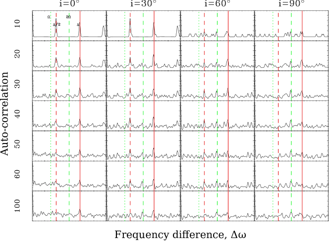
Figure 2: (colour online) Auto-correlation functions of acoustic spectra in a 2 $M_{\odot}$ stellar model rotating at $0.5\,\Omega_{\mathrm{C}}$. The spherical radial orders of the modes, $n$, range from $2$ to $9$, therefore spanning $7$ large frequency separations. The four columns correspond to four different inclinations, $i=0^{\circ}$ being a pole-on configuration. Each row corresponds to a different number of included modes. For example, in the top row, only the $10$ most visible modes are included in the frequency spectra before calculating the auto-correlation function. The vertical dotted and dashed green lines give the rotation rate, $\Omega$, and twice its value. The vertical dashed and continuous red lines indicate the large frequency separation, $\Delta$, and half its value (see Eqs. 2 and 3).

Figure 3 shows what happens with a model rotating at $0.7\,\Omega_{\mathrm{C}}$. This time, the large frequency separation is very similar to twice the rotation rate. As a result, the auto-correlation functions show very strong peaks at both $\Delta\simeq 2\Omega$ and $\Delta/2\simeq\Omega$, regardless of the inclination angle. This is not surprising as the corresponding regularities add up to produce strong peaks. The pulsation frequencies actually tend to cluster around points separated by $\Delta/2\simeq\Omega$. While such regularities are then easier to spot, it is difficult to disentangle between changing the pseudo-radial order, $\tilde{n}$, and changing the azimuthal order. A similar coincidence occurs around $0.3\Omega_{\mathrm{C}}$ where $2\Omega$ is close to $\Delta/2$. This also leads to strong peaks in the auto-correlation functions.

It is interesting to observe that the frequency spacing $\Omega\simeq\Delta/2$ shows up quite strongly in Fig. 3, even in the equator-on ($i=90^{\circ}$) configuration. This is somewhat surprising since antisymmetric modes cancel out, only leaving even modes which are spaced by $\Delta$ for fixed values of $(\tilde{\ell},\,m)$. Furthermore, prograde and retrograde modes with $m=\pm 1$ are spaced by $2\Omega$. The explanation lies in the fact that if one considers a “multiplet” of modes with the same $(\tilde{n},\,\tilde{\ell})$ values, at sufficient rotation rates, modes with consecutive $m$ values are approximately separated by $\Omega$, at least for small values of $|m|$. Indeed, the advection term $m\Omega$ is much stronger than the frequency deviations in the corotating frame which behaves as $m/\sqrt{\tilde{n}}$ according to the numerical calculations of Reese et al. (2009a) and the analytical model of Pasek et al. (2012).

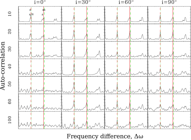
Figure 3: (colour online) Same as Fig. 2 except that the model is rotating at $0.7\,\Omega_{\mathrm{C}}$.

4.3 Inclusion of random factors

Here, we multiplied the mode visibilities from the previous case by random numbers, before selecting the highest-amplitude modes and calculating the auto-correlation functions. The random numbers are between 1 and 100 and are uniformly distributed on a logarithmic scale. Figure 4 shows the resultant auto-correlation functions for a model rotating at $0.7\,\Omega_{\mathrm{C}}$. As can be seen, the signature of regularities are much less evident than previously. Nevertheless, some peaks still remain, for instance the peak around $\Delta$ for $i=30^{\circ}$ with $30$ modes and the peak around $\Delta/2$, and to a lesser extent $\Delta$, for $i=60^{\circ}$ with $200$ or $300$ modes. Similar signatures occurs around $0.3\Omega_{\mathrm{C}}$ where $2\Omega$ is close to $\Delta/2$. However, away from the coincidences between $2\Omega$ and $\Delta$ or $\Delta/2$, the multiplication of the mode amplitude by such a random factor makes the characteristic frequency separations much more difficult to extract.

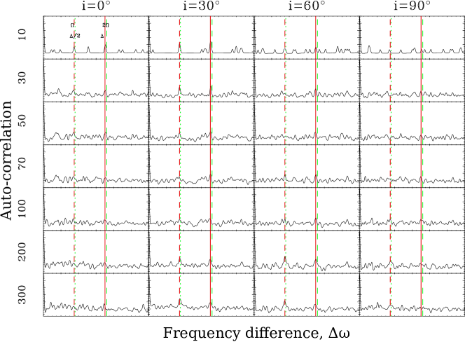
Figure 4: (colour online) Same as Fig. 2 except that the model is rotating at $0.7\,\Omega_{\mathrm{C}}$, and the visibilities have been multiplied by random numbers between $1$ and $100$ (which therefore affects which modes are selected in the frequency spectra).

4.4 Other normalisations

Figure 5 shows how the auto-correlation functions are modified when using the normalisation based on the kinetic energy. Qualitatively, this remains the same as Fig. 2. Some of the peaks stand out better, notably the $2\Omega$ peaks for few modes. In contrast, the normalisation based on the mean surface displacement (not shown) gives poor results. The explanation for this is quite simple: by normalising by the mean surface displacement, gravity (or gravito-inertial) modes are no longer penalised. Furthermore, the $(\omega+m\Omega)^{2}$ factor in Eq. (10) ends up amplifying them. Hence, the spectra of selected modes based on this normalisation are dominated by gravity modes, which do not follow the same pattern, thereby drowning out the $\Delta$, $\Delta/2$, $\Omega$, and $2\Omega$ signatures in most cases.

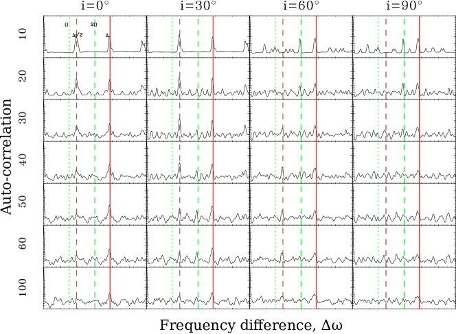
Figure 5: (colour online) Same as Fig. 2 (i.e. with a model rotating at $0.5\Omega_{\mathrm{C}}$) but where the modes are normalised by the kinetic energy, multiplied by the appropriate power of $(\omega+m\Omega)$.

5 Fourier transform of the frequency spectrum

5.1 General description

Recently, García Hernández et al. (2009, 2013) and García Hernández et al. (2015) analysed the Fourier transforms of the frequency spectra of the $\delta$ Scuti stars HD 174936 and HD 174966, observed by CoRoT. They investigated what happens when the number of selected frequencies varies from a few tens to a few hundreds. In what follows, we apply the same procedure but to our numerically calculated frequency spectra. We select modes according to their visibilities in CoRoT’s photometric band, then assign the same amplitude to the selected modes before calculating the Fourier transform of the resultant spectrum. In order to facilitate comparisons with the auto-correlation functions, we apply this technique to the frequency spectra spanning 7 radial orders, studied the previous section (i.e. Figs. 2 and 3).

5.2 Normalisation of the maximal displacement

Figure 6 shows the squared modulus of the Fourier transform of frequency spectra in the model rotating at $0.5\,\Omega_{\mathrm{C}}$, for various numbers of selected modes and for four different inclinations. Taking the Fourier transform of a function which depends on frequency yields another function which depends on time $t$; it is plotted here as a function of $1/t$ to facilitate the identification of regularities. At low inclinations, peaks appear at $\Delta/2$ with their forest of harmonics at $\Delta/4$, $\Delta/6$, etc. This can be expected because the frequency spectrum is behaving like a Dirac comb with a $\Delta/2$ periodicity. At higher inclinations, a peak appears close to $\Delta$ (that is an expected regularity), but is shifted; we also recover some harmonics (especially at $\Delta/3$), but not all of them. This is probably an effect of rotation that does not necessarily add peaks but acts as a modulation of the amplitude of the Fourier transform. Indeed, we notice that rotation does not produce peaks at $2\Omega$ or $\Omega$. This is because, although there are recurrent frequency separations of $2\Omega$ (or actually slightly smaller because of the Coriolis force), such separations are formed by pairs of frequencies rather than by a Dirac comb. Nevertheless, when the frequency spectrum is dominated by two similar subspectra, the second one being identical to the first one but shifted by $2\Omega$ (this is what happens when $m=\pm 1$ modes dominate), the Fourier transform of the full spectrum will be the Fourier transform of the subspectrum multiplied by $\cos^{2}(\Omega t)$. Such a modulation can make some peaks disappear or slightly shift some broad peaks. In such a configuration, it is impossible to unambiguously detect the correct large separation with the Fourier transform only.

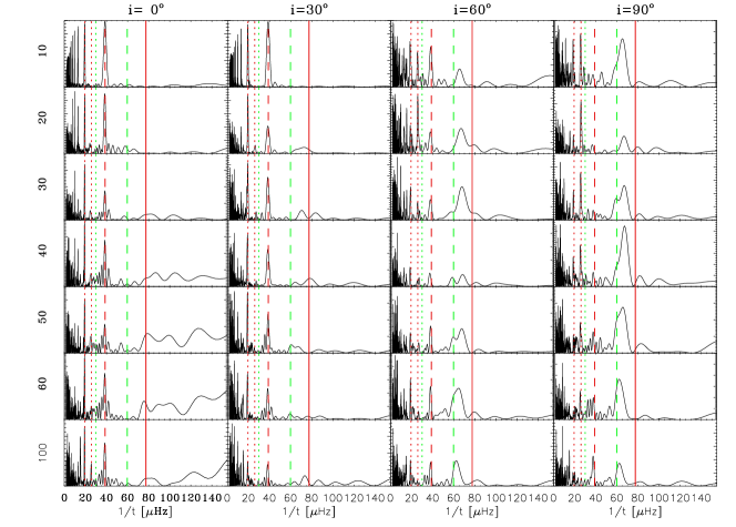
Figure 6: (colour online) Fourier transform of frequency spectra in a $2\,M_{\odot}$ model rotating at $0.5\,\Omega_{\mathrm{C}}$. Each row corresponds to a different number of selected modes, as indicated on the left, and each column to a different inclination, as stated above. The red, continuous and discontinuous, vertical lines correspond to the large frequency separation, $\Delta$, and various fractions of this value: $\Delta/4$, $\Delta/3$ and $\Delta/2$. The green, dotted and dashed, vertical lines correspond to $\Omega$ and $2\Omega$, respectively.

Figure 7 shows what happens with the model rotating at $0.7\,\Omega_{\mathrm{C}}$, where $\Delta$ nearly coincides with $2\Omega$. In this case, the frequency spectra take on a fairly simple form in which the frequencies cluster around points separated by $\Delta/2\simeq\Omega$, regardless of inclination. This leads to strong peaks at $\Delta/2$ and $\Delta/4$ in the Fourier transforms, regardless of inclination.

Figure 7: (colour online) Same as Fig. 6 but for a model rotating at $0.7\,\Omega_{\mathrm{C}}$.

5.3 Other normalisations

Figure 8 shows the effects of the alternative normalisations described in Sect. 4.1 on the Fourier transform of the spectra of the $\Omega=0.5\Omega_{\mathrm{C}}$ and $\Omega=0.7\Omega_{\mathrm{C}}$ models. The Fourier transforms continue to detect $\Delta/2$ and its many harmonics in many cases, even when using random factors or the normalisation based on the mean surface displacement. However, the tests involving random factors benefit from the coincidence between $\Delta$ and $2\Omega$. In the absence of such a coincidence, the $\Delta/2$ signature is far less visible, except in a few cases where it still shows up. Overall, these tests confirm the robustness of the large and semi-large frequency separations as detected by the Fourier transform to different non-random normalisations, or when examining favourable cases where $\Omega$ coincides with $\Delta/2$ or $\Delta$.

Inclusion of random factors ($\Omega=0.7\Omega_{\mathrm{C}}$)

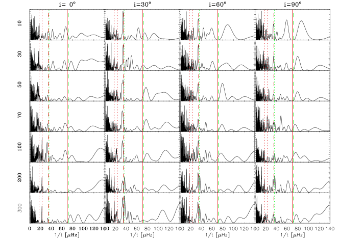
Mean surface displacement normalisation ($\Omega=0.5\Omega_{\mathrm{C}}$)

Figure 8: (colour online) Same as Fig. 6 but where the mode normalisation includes random factors (top panel) or is based on the mean surface displacement (bottom panel).

Overall, the Fourier transforms complement the auto-correlation functions quite nicely. Indeed, although both detect the separation $\Delta/2$, only the auto-correlation functions are sensitive to $2\Omega$. As explained above, such frequency separations are produced by pairs of modes rather than by Dirac combs thereby escaping detection by Fourier transforms, but not by the auto-correlation functions. Hence, this provides a simple way to distinguish between the two and to get a better grasp of the regularities present in the spectrum.

6 Multi-colour mode identification

6.1 Method

We now turn our attention to multi-colour mode identification. As was emphasised in the introduction, multi-colour mode signatures, such as the ratios between mode amplitudes observed in different photometric bands, do not depend on intrinsic mode amplitudes since these factor out. In Paper I, it was shown that such amplitude ratios tend to be similar for island modes with the same $(\ell,\,|m|)$ values, even in the most rapidly rotating models. This is consistent with the fact that such modes have a similar surface structure (see Section 2). Hence, this raises the question as to whether we can select modes with similar properties by picking a reference mode at random in an oscillation spectrum and searching for the $N$ other modes which produce the most similar amplitude ratios. In what follows, we will use the following cost function to evaluate the proximity of a mode’s amplitude ratios to that of the reference mode:

$$J=\sum_{i=1}^{d}\left(V_{i}-V_{i}^{\mathrm{ref}}\right)^{2},$$ (11)

where $i$ is an index on the photometric band, $d$ the number of photometric bands, $V_{i}^{\mathrm{ref}}$ the visibilities of the reference mode and $V_{i}$ those of the mode being evaluated. The visibilities have been normalised using $\sum_{i=1}^{d}V_{i}^{2}=\sum_{i=1}^{d}\left(V_{i}^{\mathrm{ref}}\right)^{2}=1$ to avoid favouring a particular photometric band. Nonetheless, a small value for $J$ implies that the $V_{i}$’s are close to the $V_{i}^{\mathrm{ref}}$’s and therefore that the amplitude ratios are similar.

This approach is different than the one typically taken in other works such as Daszyńska-Daszkiewicz et al. (2002). Indeed, most authors compare observed amplitude ratios directly with theoretical ones. The approach described here consists in comparing observed amplitude ratios between each other. It thus bypasses limitations in the theoretical predictions. In the following, we shall nevertheless use theoretical amplitude ratios to test its validity.

6.2 Adiabatic case

We start with the $(n,\,\ell,\,m)=(9,4,1)$ mode in the model at $0.6\,\Omega_{\mathrm{C}}$ as the reference mode and search for the $9$ other modes with the most similar amplitude ratios. The mode visibilities are calculated using the Geneva photometric system, which contains seven photometric bands. Before normalising the visibilities, we filter out modes where the overall visibility is more than 100 times smaller than that of the reference mode, thereby excluding most gravity modes. Figure 9 shows the results for $i=60^{\circ}$. In the first row, the left panel shows the amplitude ratios, the dashed line corresponding to the reference mode (we note that this line is hardly visible because it is mostly covered up by the solid lines from the other modes), the middle panel gives the frequencies, where a higher rank indicates a higher resemblance with the reference mode, $10$ corresponding to the reference mode, and the right panel displays the auto-correlation function of the sub-spectrum of the selected frequencies. The second and third rows show the meridional cross-sections of the selected modes. Beneath each mode, the values of $(n,\,\ell,\,m)$ are indicated when the mode corresponds to an $\tilde{\ell}<2$ island mode. Otherwise, only the azimuthal order, $m$, is provided.

Figure 9: (colour online) Amplitude ratios, frequency spectrum and ranks, associated auto-correlation function, and meridional cross-sections of the reference mode $(n,\,\ell,\,m)=(9,4,1)$ and the $9$ other most similar modes, for an inclination of $i=60^{\circ}$ – see text for details.

The results shown in Fig. 9 are promising. Apart from the mode at $5.124$ $\Omega_{\mathrm{K}}$, all of the modes belong to the $(\ell,\,|m|)=(4,1)$ family of island modes. This then leads to clear peaks in the auto-correlation function at $2\Omega$, $\Delta$, and $2\Delta$, as well as combination peaks at $\Delta-2\Omega$, $2\Delta-2\Omega$, and $\Delta+2\Omega$. Another example of highly successful mode selection using the same strategy can be found in Figure 4 of Reese et al. (2013a). However, not all cases work out so well.

To get a global picture of the mode selection method, we applied it to all of the identified island modes above a given threshold frequency in the pulsation spectrum of our 2 $M_{\odot}$, 0.6 $\Omega_{\mathrm{C}}$ stellar model. Then, we quantified the mode selection success rate by finding the average number of island modes (excluding the reference mode), the average number of island modes with the same $(\ell,\,|m|)$ values as the reference mode, and the average number of island modes with the same $(\tilde{\ell},\,|m|)$ values, all of which are subsequently divided by the total number of selected modes, i.e. $N=9$, to get a success rate comprised between $0$ and $1$.

Results are given in columns 2-4 of Table 1, for a threshold frequency $\omega_{\mathrm{threshold}}=8.0\,\Omega_{\mathrm{C}}$. In this case, the total number of island modes divided by the total number of modes is $0.0115$. Thus, the much higher success rates obtained show that selecting modes according to similar amplitude ratios considerably increases the chances of finding island modes, provided the reference mode is an island mode. When the inclination is high, the method selects island modes of the same parity. In contrast, in near pole-on configurations, it will select modes of both equatorial symmetries. This property explains the difference in the $(\ell,\,m)$ versus $(\tilde{\ell},\,m)$ success rates. Repeating this test for different values of the threshold frequency shows that higher success rates are achieved for higher frequency modes, most probably because they are further into the asymptotic regime.

Table 1: Overall success rate in finding similar modes via the multi-colour mode identification scheme.

	Adiabatic (2 M⊙)			Adiabatic (1.8 M⊙)			Pseudo non-adiabatic (1.8 M⊙)
Orientation	Island	Same $(\ell,\,|m|)$	Same $(\tilde{\ell},\,|m|)$	Island	Same $(\ell,\,|m|)$	Same $(\tilde{\ell},\,|m|)$	Island	Same $(\ell,\,|m|)$	Same $(\tilde{\ell},\,|m|)$
All	0.564	0.359	0.416	0.554	0.401	0.452	0.469	0.303	0.349
$i=0^{\circ}$	0.519	0.241	0.519	0.594	0.256	0.594	0.633	0.256	0.633
$i=30^{\circ}$	0.474	0.268	0.375	0.483	0.343	0.430	0.441	0.303	0.357
$i=60^{\circ}$	0.643	0.444	0.450	0.600	0.449	0.449	0.485	0.323	0.340
$i=90^{\circ}$	0.597	0.402	0.402	0.592	0.462	0.462	0.450	0.275	0.275

Overall, the method appears to be a promising way of choosing modes with similar surface distributions and hence quantum numbers. Regularities of the sub-spectrum of selected modes may then help to determine the azimuthal order, thanks to the frequency separations $2|m|\Omega$, and constrain the radial order. Nonetheless, one may still wonder if such a strategy will continue to work when non-adiabatic effects are taken into account. In what follows we examine this question by analysing mode visibilities in which non-adiabatic effects are approximated.

6.3 Pseudo non-adiabatic effects

Non-adiabatic effects strongly modify the effective temperature variations and, hence, multi-colour photometric signatures of pulsation modes. One may then wonder if such effects are able to mask the structural similarities between modes with similar quantum numbers and thus alter the promising results of the mode selection method obtained in the adiabatic case. In the absence of full non-adiabatic pulsation calculations in rapidly rotating $\delta$ Scuti stars, we shall use non-adiabatic calculations in the non-rotating case to derive approximate non-adiabatic visibilities in the rotating case.

In non-rotating stars, the relative effective temperature fluctuations are typically proportional to the radial displacement:

$$\frac{\delta T_{\mathrm{eff}}}{T_{\mathrm{eff}}}=\frac{\xi_{r}}{R^{\star}}f_{T}\exp(i\phi_{T})$$ (12)

where $R^{\star}$ is the radius of the non-rotating model. The quantity $f_{T}\exp(i\phi_{T})$ represents the non-adiabatic effects and generally depends on the degree $\ell$ and frequency $\omega/\Omega_{\mathrm{K}}$ of the mode, as well as on the effective temperature and surface gravity. However, as illustrated in Fig. 10, it actually depends little on the harmonic degree for acoustic modes (i.e. at sufficiently high frequencies). We also note that, when described as a function of $\omega/\Omega_{\mathrm{K}}$, $f_{T}\exp(i\phi_{T})$ is only slightly affected by the effective gravity as can be seen by comparing the two models in Fig. 10, except at high frequencies, where the effect is somewhat stronger. In a rotating star, the effective temperature and the surface gravity vary from pole to equator. Hence, to estimate non-adiabatic effects, we calculated, using the MAD code (Dupret, 2001), $f_{T}\exp(i\psi_{T})/R^{\star}$ for a set of non-rotating models along four evolutionary sequences, which span the effective temperature and surface gravity ranges of our rotating models, and for a set of modes spanning the relevant frequency range. We smoothed out the small differences in degree and interpolated according to frequency, effective temperature, and effective gravity, so as to have a value for $f_{T}\exp(i\phi_{T})/R^{\star}$ at each co-latitude for each frequency. The function $|f_{T}|/R^{\star}$ is shown in Fig. 11. This was subsequently multiplied by $R(\theta)$, the radius of the rotating model which depends on the co-latitude, $\theta$, and then applied at the corotating pulsation frequency, $(\omega+m\Omega)/\Omega_{K}$ in order to estimate the effective temperature variations arising in our pulsating rotating models. A quick look at the function $|f_{T}|/R^{\star}$ shows that it cannot simply be expressed as the product of a function which depends on $\theta$ alone and another function which depends on frequency alone, i.e. it is non-separable in terms of these two variables. Accordingly, this will distort the $\theta$ dependence of $\delta T_{\mathrm{eff}}/T_{\mathrm{eff}}$ as the frequency changes, thereby leading to increased scatter in the photometric signatures of a given $(\ell,\,|m|)$ family of island modes.

Figure 10: (Colour online) The quantities $f_{T}$ and $\phi_{T}$ in two non-rotating models with masses 1.8 $M_{\odot}$ and 2.0 $M_{\odot}$. The two models nearly have the same temperature (8143.9 K and 8137.3 K, respectively), but different $\log(g)$ values (4.1249 dex and 3.9593 dex, respectively). The different line styles correspond to different $\ell$ values, and the overlapping vertical dotted lines (which are hard to distinguish) indicate the position of the fundamental modes of both models.

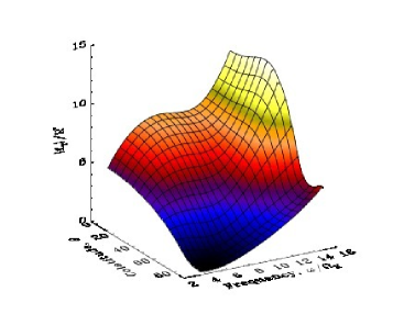
Figure 11: (Colour online) The quantity $|f_{T}|/R^{\star}$ as a function of co-latitude and frequency, for the 1.8 $M_{\odot}$ rotating model.

Adiabatic case

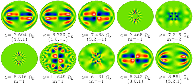
Pseudo non-adiabatic case

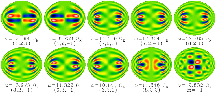
Figure 12: (Colour online) Same as Fig. 9 but for the reference mode $(n,\,\ell,\,m)=(4,2,1)$ (and for both the adiabatic and pseudo non-adiabatic case).

As in the previous section, the method to find similar modes is applied to all of the island modes above a frequency threshold of $8.0\,\Omega_{\mathrm{C}}$ and its efficiency is quantified by computing an overall success rate. In Table 1 the adiabatic results for a rotating model, $M=1.8\,M_{\odot}$, $\Omega=0.6\,\Omega_{\mathrm{C}}$, (see columns 5-7) are compared with the pseudo non-adiabatic ones (columns 8-10). In the present case, the number of island modes divided by the total number of modes is $0.0330$. Table 1 shows that pseudo non-adiabatic success rates are worse than adiabatic ones but the method remains efficient in selecting island modes, when island modes are used as reference modes.

There are a number of cases where pseudo non-adiabatic calculations lead to similar or even better results than the adiabatic calculations, such as the case illustrated in Fig. 12. In the adiabatic case, five of the selected modes are not island modes, even though the reference mode is an island mode. In the pseudo non-adiabatic case, only one of the selected modes is not an island mode, and there is also one island mode with a different value of $|m|$. The remaining modes correspond to pairs of $(\ell,|m|)=(2,1)$ island modes. This gives rise to strong signatures at $2\Omega$, $\Delta$ and $2\Delta$, as well as some combination peaks in the auto-correlation function.

Hence the technique appears to remain viable in the non-adiabatic case. Furthermore, phase differences (e.g. Balona & Evers, 1999; Dupret et al., 2005) could also be exploited and may lead to higher success rates by providing supplementary constraints. This can, however, only be tested when full non-adiabatic pulsation calculations are available in rapidly rotating $\delta$ Scuti stars, since it is only in such conditions that phase differences can be obtained with a reasonable accuracy.

7 Conclusion

In this paper, we investigated different ways of applying the visibility calculations of Reese et al. (2013b) to the interpretation of pulsation spectra in rapidly rotating stars. Given the lack of a comprehensive theory on non-linear mode saturation in $\delta$ Scuti stars, we tested various ad-hoc assumptions in order to determine intrinsic mode amplitudes. As such, these results must be taken with caution but represent a first step towards interpreting pulsation spectra in such stars using realistic mode visibilities.

We first looked at the auto-correlation functions of frequency spectra in much the same way as had been done in Lignières et al. (2010), but using the newer more realistic visibilities, applied to spectra of acoustic modes calculated in a self-consistent way (rather than having the non-axisymmetric modes estimated from the axisymmetric ones). Our results confirm those of Lignières et al. (2010) in the sense that it is possible to observe peaks corresponding to a mean value of the large frequency separation, $\Delta$, half its value, $\Delta/2$, the rotation rate, $\Omega$, and twice the rotation rate, $2\Omega$, when conditions are favourable. Such conditions are achieved when the frequencies span a large enough range to reinforce recurrent spacings, and when not too many modes are included. The orientation of the star is important as it will favour either $\Delta/2$ for low inclinations (i.e.  close to pole-on), or $\Delta$ and $2\Omega$ for high inclinations. The $\Omega$ spacing is visible due to the usual multiplet structure at small rotation rates, then it disappears and becomes visible again at high rotation rates when a new of type multiplet forms. Of particular interest are the situations where $2\Omega$ coincides with either $\Delta/2$ or $\Delta$, which occurs for models rotating at $0.3\,\Omega_{\mathrm{C}}$ or $0.7\,\Omega_{\mathrm{C}}$, respectively. Such situations lead to a very strong signature in the auto-correlation function, due to a simplification of the spectrum in which modes tend to cluster together. Although this is ideal for detecting those frequency separations, it also makes it more difficult to disentangle the two. Finally, we experimented with multiplying the intrinsic amplitudes by random numbers between $1$ and $100$, uniformly spread out on a logarithmic scale. This is used as a poor substitute for the effects of non-linear saturation and mode coupling on the amplitudes in such stars. In spite of that, a weak signature of the frequency separations remained in the favourable case where $\Delta$ coincided with $2\Omega$. This gives hope that it may be possible to detect, at least in favourable cases, such characteristic separations, and might explain the recent detection of recurrent spacings in $\delta$ Scuti stars (Mantegazza et al., 2012; Suárez et al., 2014; García Hernández et al., 2009, 2013, 2015).

We also looked at Fourier transforms of the frequency spectra. Although these also detected $\Delta/2$ as a recurrent spacing, $2\Omega$ escaped detection. This is because the latter are not formed by a Dirac comb, but rather by isolated pairs of frequencies. This difference between the two approaches is quite useful as it helps us distinguish between the two types of separations. Hence, one can hope to interpret observed spectra by combining the two approaches and correctly identifying $\Delta/2$ and $2\Omega$. Further tests based on different mode normalisations confirmed the robustness of both the auto-correlation functions and the Fourier transforms at detecting these characteristic frequency separations, as long as gravito-inertial modes were excluded from the analysis.

Finally, we turned our attention to multi-colour mode identification. A key advantage of multi-colour mode signatures, such as amplitude ratios, is that the intrinsic amplitudes factor out, thereby leaving a signature which is only sensitive to the geometric structure of the mode. Previous investigations into the matter had concluded that, due to the dependence of amplitude ratios on inclination and azimuthal order, it would be very difficult to identify modes in rapidly rotating stars from multi-colour photometry alone (e.g. Daszyńska-Daszkiewicz et al., 2002; Townsend, 2003). In contrast, we present more promising results. To achieve this, we apply a strategy different from the non-rotating case, a strategy which involves choosing a reference mode and searching for other modes with the most similar amplitude ratios. By repeating this procedure for different reference modes, we can group modes together into families with similar amplitude ratios. It turns out that such families have similar azimuthal orders and degrees, and their frequencies follow patterns which help to constrain the identification of these modes as well as the rotation rate and the large frequency separation. Furthermore, by comparing modes between each other rather than with theoretical predictions, one bypasses the current limitations with our theory such as the lack of full 2D non-adiabatic pulsation calculations, or the difficulties in modelling the interactions between such modes and convection. Nonetheless, we investigated, in an approximate way, non-adiabatic effects on multi-colour mode amplitudes. It was found that non-adiabatic effects do tend to increase the scatter between the multi-colour photometric signatures of similar modes due to its distortion of $\delta T_{\mathrm{eff}}/T_{\mathrm{eff}}$ as a function of frequency. This makes the above mode identification strategy more difficult to apply although some of the results still remain promising. Even if it turned out to be too penalising for mode identification, it would still be possible to extract recurrent spacings such as the rotation rate, and possibly the large frequency separation.

Of course, for multi-colour mode identification to work well, one needs high quality multi-colour photometric observations of stars with numerous pulsation modes, such as $\delta$ Scuti stars. In this regard, the constellation of nano-satellites, BRITE (Kuschnig et al., 2009), is a promising source of such data, given that it observes in red and blue photometric bands. The PLATO mission, scheduled for launch in $2025$, will contain a platform of $26$ telescopes, two of which will include broadband filters and the remaining $24$ will operate in white light (Catala et al., 2011; Rauer et al., 2014).