Asymptotically Efficient Identification of Known-Sensor Hidden Markov Models

Abstract

We consider estimating the transition probability matrix of a finite-state finite-observation alphabet hidden Markov model with known observation probabilities. The main contribution is a two-step algorithm; a method of moments estimator (formulated as a convex optimization problem) followed by a single iteration of a Newton-Raphson maximum likelihood estimator. The two-fold contribution of this letter is, firstly, to theoretically show that the proposed estimator is consistent and asymptotically efficient, and secondly, to numerically show that the method is computationally less demanding than conventional methods – in particular for large data sets.

I Introduction

The hidden Markov model (HMM) has been applied in a diverse range of fields, e.g., signal processing [1], gene sequencing [2, 3] and speech recognition [4]. The standard way of estimating the parameters of an HMM is by employing a maximum likelihood (ML) criterion. However, numerical “hill climbing” algorithms for computing the ML estimate, such as direct maximization using Newton-Raphson (and variants, e.g., [5]) and the expectation-maximization (EM, e.g, [6, 4]) algorithm are, in general, only guaranteed to converge to local stationary points in the likelihood surface. It is also known that these schemes can, depending on the initial starting point of the algorithms, the shape of the likelihood surface and the size of the data set, exhibit long run-times.

An alternative to ML criterion is to match moments of an HMM, resulting in a method of moments estimator (see, e.g. [7] for details). In such a method, observable correlations in the HMM data are related to the parameters of the system. The correlations are empirically estimated and used in the inverted relations to recover parameter estimates. A number of methods of moments for HMMs have been proposed in the recent years, e.g., [8, 9, 10, 11, 12, 13, 14]. The main benefits over iterative ML schemes are usually consistency and a shorter run-time, however, typically since only low-order moments are considered, there is a loss of efficiency in the resulting estimate.

In the present letter, the problem of estimating the transition probabilities of a finite discrete-time HMM with known sensor uncertainties, i.e., observation matrix, is considered. This setup can be motivated in two ways: firstly, it can be seen as the second step in a decoupling approach to learning the HMM parameters (see [11]), or alternatively, by any application where the sensor used to measure the system is designed/known to the user.

The main idea in this letter is a hybrid two-step algorithm based on combining the advantages of the two aforementioned approaches. The first step uses a method of moments estimator which requires a single pass over the data set (compared to iterative algorithms, such as EM, that require multiple iterations over the data set). The second step uses the method of moments estimate to initialize a non-iterative second-order direct likelihood maximization procedure. This allows us to avoid resorting to ad hoc heuristics for localizing a good starting point. More importantly, we show that it is sufficient to perform only a single iteration of the ML procedure to obtain an asymptotically efficient estimate. Put differently, only two passes through the data set are necessary in order to obtain an asymptotically efficient estimate.

To summarize, the main contributions of this letter are:

• a proposed two-step identification algorithm that exploits the benefits of both the method of moments approach (low computational burden and consistency) and direct likelihood maximization (high accuracy);

• we prove the consistency and asymptotic efficiency of the proposed estimator. Hence, the problem of only local convergence that may haunt iterative ML algorithms, such as EM, is shown to be avoided;

• numerical studies that show that the proposed method is up to an order of magnitude faster than the standard EM algorithm – with the same resulting accuracy (when the EM iterations approach the global optimum of the likelihood function). Moreover, the run-time is, roughly, constant for a fixed data size, whereas the run-time of EM is highly dependent on the data (due to the number of iterations needed for convergence).

The outline of the remaining part of this letter is as follows. We first present a brief overview of related work below. Section II then poses the problem formally and Section III presents the algorithm. In Section IV asymptotical efficiency is proven, and Section V presents numerical studies.

Related Work

HMM parameter estimation is now a classical area (with more than 50 years of literature). There has recently been interest in the machine learning community for employing methods of moments for HMMs. The method presented in [10, Appendix A] demonstrates how to recover explicit estimates of the transition and observation matrices by exploiting the special structure of the moments of an HMM. This method has been further generalized and put in a tensor framework; see, e.g., [9], [12] and references therein. The appealing attribute of these methods is that they generate non-iterative estimates using simple linear algebra operations (eigen and singular-value decompositions). However, the non-negativity and sum-to-one properties of the estimated probabilities cannot be guaranteed.

There are a number of proposed methods of moments for HMMs formulated as optimization problems (which allow constrains to be forced on the estimates), e.g., [8], [11] and [14]. The identification problem is decoupled in [11] into two stages: first an estimation of the output parameters, and then a moment matching optimization problem. The resulting optimization problem is related to the one in [8] and to the problem in the present work. The method we propose in this letter could be seen as a possible improvement of the second step in the setting of [11].

In the general setting, hybrid approaches, such as the combination of EM and direct likelihood maximization, and other attempts to accelerate EM has been studied in, e.g., [15, 16]. Iterative direct likelihood maximization for HMMs, as well as methods for obtaining the necessary gradient and Hessian expressions, are treated in, e.g., [17, 18, 5, 19, 20, 21]. The combination of a method of moments and EM has, in the case of HMMs, been considered in [11].

II Preliminaries and Problem Formulation

All vectors are column vectors unless transposed, $\mathds{1}$ denotes the vector of all ones. The vector operator $\text{diag}:\mathbb{R}^{n}\rightarrow\mathbb{R}^{n\times n}$ gives the matrix where the vector has been put on the diagonal, and all other elements are zero. $\|\cdot\|_{F}$ denotes the Frobenius norm of a matrix. The element at row $i$ and column $j$ of a matrix is $[\cdot]_{ij}$, and the element at position $i$ of a vector is $[\cdot]_{i}$. Inequalities ($>,\geq,\leq,<$) between vectors or matrices should be interpreted elementwise. The indicator function $\text{I}\{\cdot\}$ takes the value 1 if the expression $\cdot$ is fulfilled and 0 otherwise. Let $\to_{p}$ and $\to_{d}$ denote convergence in probability and in distribution, respectively, and let $\mathcal{O}_{p}$ and $o_{\text{p}}$ be stochastic-order symbols. $\sim$ denotes “distributed according to”.

II-A Problem Formulation

Consider a discrete-time finite-state hidden Markov model (HMM) on the state space $\mathcal{X}=\{1,2,\dots,X\}$ with the transition probability matrix

$$[P]_{ij}=\operatorname{Pr}[x_{k+1}=j|x_{k}=i].$$ (1)

Observations are made from the set $\mathcal{Y}=\{1,2,\dots,Y\}$ according to the observation probability matrix

$$[B]_{ij}=\operatorname{Pr}[y_{k}=j|x_{k}=i].$$ (2)

These matrices are row-stochastic, i.e., the elements in each row sum to one. Denote the initial distribution as $\pi_{0}$ and the stationary distribution as $\pi_{\infty}$.

The HMM moments are joint probabilities of tuples of observations. The second order moments can be represented by $Y\times Y$ matrices $M_{k}$ with elements

$$[M_{k}]_{ij}=\operatorname{Pr}[y_{k}=i,y_{k+1}=j].$$ (3)

The following equation relates the second order moments and the system parameters,

$$M_{k}=B^{T}\operatorname{diag}((P^{T})^{k}\pi_{0})PB,$$ (4)

and is the key to the method of moments formulation of the problem.

As we are interested in the asymptotic behaviour, we make the assumption that the initial distribution $\pi_{0}$ is known to us – its influence will anyway diminish over time. The most important assumption we make is that the observation probabilities $B$ are known. There are three motivations for this assumption: i) it admits the problem to a convex formulation, ii) it holds in any real-world application where the sensor is designed by the user, and iii) our method can be seen as an intermediate step of the decoupling approach in [11]. The identification problem we consider is, hence,

Problem 1.

Consider an HMM with known initial distribution $\pi_{0}$ and known observation matrix $B$. The HMM is initialized according to $\pi_{0}$ and a sequence of observations $y_{0},y_{1},\dots,y_{N}$ is obtained. Given the sequence of $N+1$ observations $\{y_{k}\}_{k=0}^{N}$, estimate the transition matrix $P$.

III Asymptotically Efficient Two-Step Algorithm

In this section, we outline the two-step algorithm which is the main contribution of this letter.

Step 1. Initial Method of Moments Estimate

In light of (3), use the empirical moments estimate

$$[\hat{M}_{\infty}]_{ij}=\frac{1}{N}\sum_{k=0}^{N-1}\text{I}\{y_{k}=i,y_{k+1}=j\},$$ (5)

for the (stationary) second order moments.

In the moment matching optimization problem, we need to impose the constraint that the transition matrix is a valid stochastic matrix, that is: the non-negativity and sum-to-one properties of its rows. We require that the transition matrix of the HMM is ergodic (aperiodic and irreducible). This implies, first of all, that $\pi_{\infty}$ is the right eigenvector of $P^{T}$ and therefore satisfies the condition $\pi_{\infty}=P^{T}\pi_{\infty}$, and secondly, that $\pi_{\infty}$ has strictly positive entries. We therefore, also, include in the optimization problem a polytopic bound $\underaccent{\bar}{\Pi}$ on $\pi_{\infty}$ such that for a vector $x\in\underaccent{\bar}{\Pi}\Rightarrow x>0$.

To summarize, estimating the transition matrix $P$ involves solving the optimization problem (as the limit is taken in equation (4) towards stationarity):

$$\min_{\pi_{\infty},P} \quad\|\hat{M}_{\infty}-B^{T}\operatorname{diag}(\pi_{\infty})PB\|_{F}^{2}$$

s.t. $$\quad P\geq 0,\;\;\;\quad\pi_{\infty}\geq 0,$$

$$\quad P\mathds{1}=\mathds{1},\quad\mathds{1}^{T}\pi_{\infty}=1,$$

$$\quad\pi_{\infty}\in\underaccent{\bar}{\Pi},\quad\pi_{\infty}=P^{T}\pi_{\infty}.$$ (6)

This is, in general, a non-convex optimization problem. The lemma below shows that convex optimization techniques can be used to solve the problem.

Lemma 1.

The solution of problem (6) is obtainable by solving the convex problem

$$\min_{A}\quad \|\hat{M}_{\infty}-B^{T}AB\|_{F}^{2}$$

s.t. $$A\geq 0,\mathds{1}^{T}A\mathds{1}=1,$$

$$A\mathds{1}\in\underaccent{\bar}{\Pi},A\mathds{1}=A^{T}\mathds{1},$$ (7)

and using (9) and (10), see below, to recover $\pi_{\infty}$ and $P$ from the variable $A$.

Proof.

In problem (7), we identify the product $\operatorname{diag}(\pi_{\infty})P$ in problem (6) as a new parameter $A$, i.e.,

$$A=\operatorname{diag}(\pi_{\infty})P,$$ (8)

and optimize over its elements instead of over $\pi_{\infty}$ and $P$ jointly. Notice that it is possible to recover $\pi_{\infty}$ and $P$ from $A$ as follows: Firstly, recover $\pi_{\infty}$ from

$$A\mathds{1}=\operatorname{diag}(\pi_{\infty})P\mathds{1}=\pi_{\infty},$$ (9)

employing the fact that $P\mathds{1}=\mathds{1}$. Secondly, recover $P$ from

$$\operatorname{diag}(\pi_{\infty})^{-1}A=\operatorname{diag}(\pi_{\infty})^{-1}\operatorname{diag}(\pi_{\infty})P=P.$$ (10)

The lemma follows by noting that the cost functions in problems (6) and (7) are the same, and then mapping feasible solutions between the two problems. ∎

Solving problem (7) requires only a single pass over the data to obtain $\hat{M}_{\infty}$, and then solving a data-size independent convex (quadratic) optimization problem to compute an estimate of the transition matrix $P$. The trade-off compared to ML estimation, which requires multiple iterations over the observation data set, is of course between estimation accuracy and computational cost: the method of moments outlined above employs only the second order moments and will hence have disregarded some of the information in the observed data.

Step 2. Single Newton-Raphson Step

We propose to exploit the trade-off by first obtaining an estimate of $P$ using the convex method of moments (7), and then taking a single Newton-Raphson step on the likelihood function to increase the accuracy of the estimate.

The (log-)likelihood function of the observed data is

$$l_{N}(\theta)=\log\operatorname{Pr}[\,\{y_{k}\}_{k=0}^{N}\,|\,x_{0}\sim\pi_{0};\,\theta\,],$$ (11)

where $\theta$ is a parametrization of the transition matrix $P$. Denote the estimate resulting from the method of moments (7) as $\hat{\theta}_{\text{MM}}$. Then a single Newton-Raphson step is performed as follows:

$$\hat{\theta}_{\text{NR}}=\hat{\theta}_{\text{MM}}-\big{[}\nabla_{\theta}^{2}l_{N}(\hat{\theta}_{\text{MM}})\big{]}^{-1}\;\nabla_{\theta}l_{N}(\hat{\theta}_{\text{MM}}),$$ (12)

where the gradient $\nabla_{\theta}l_{N}(\hat{\theta})$ and Hessian $\nabla_{\theta}^{2}l_{N}(\hat{\theta})$ can be computed recursively – see e.g., [17, 18, 5, 19, 20, 21].

Compared to direct maximization of the likelihood function using the Newton-Raphson method (see, e.g., [5, 19]), this procedure is non-iterative and hence, the gradient and Hessian need only to be computed once.

IV Analysis

In this section we analyze the properties of the proposed algorithm. First we state the assumptions.

Assumption 1.

The transition matrix $P$ has positive elements. The observation matrix $B$ is given, has full rank and is positive. There is a polytopic bound on $\pi_{\infty}$ such that all components of $\pi_{\infty}$ are strictly greater than zero.

The following lemma establishes (strong) consistency of the method of moments procedure.

Lemma 2.

The estimates of $P$ and $\pi_{\infty}$ obtained using (9) and (10) from problem (7) with the estimator $\hat{M}_{\infty}$ in (5), converge to their true values as the number of observations $N\rightarrow\infty$ with probability one.

Proof (outline).

The lemma follows by showing

1. that the estimate $\hat{M}_{\infty}$ converges to $M_{\infty}$ (using a law of large numbers, [5, Theorem 14.2.53]);

2. that the solution $\hat{A}$ of the optimization problem converges to $A$ (follows by the fundamental theorem of statistical learning [23, Lemma 1.1] and the convexity of the cost function [24, Theorem 10.8]);

3. that the solution of the optimization problem $\hat{A}$ can be uniquely mapped to $P$ and $\pi_{\infty}$.

Full details are available in the supplementary material. ∎

Figure 1: RMSE and run-time simulation data.

Next, we provide the main theorem of the letter.

Theorem 1.

The estimate $\hat{\theta}_{\text{NR}}$ obtained by the two-step algorithm (7)-(12) is asymptotically efficient, i.e., as $N\to\infty$,

$$\sqrt{N}(\hat{\theta}_{\text{NR}}-\theta^{*})\to_{d}\mathcal{N}(0,I_{F}^{-1}(\theta^{*})),$$ (13)

where $\mathcal{N}$ is a normal distribution, $\theta^{*}$ corresponds to the true parameters and $I_{F}$ is the Fisher information matrix.

Proof (outline).

The theorem follows by showing that

1. the estimate $\hat{M}_{\infty}$ follows a central limit theorem [25, Corollary 5], and using this, concluding that $\hat{M}_{\infty}=M_{\infty}+\mathcal{O}_{p}(N^{-1/2})$ [26, Appendix A];

2. this order in probability can be propagated through the optimization problem (7) to obtain a similar order on $\hat{P}$ and $\hat{\pi}_{\infty}$ [27, Theorem 2.1];

3. verifying that certain regularity conditions hold to ensure that we have a central limit theorem for the gradient and a law of large numbers for the Hessian matrix of the log-likelihood function [5, Theorems 12.5.5 and 12.5.6];

4. verifying by explicit computation that the single Newton-Raphson step yields an asymptotically efficient estimator.

Again, full details are available in the supplementary material.

∎

V Numerical Evaluation

In this section, we evaluate the performance of the proposed two-step algorithm and compare it to the standard EM algorithm for ML estimation. The EM implementation of Matlab R2015a was employed (modified as to account for the fact that the observation matrix is assumed known). The first step of the proposed algorithm, i.e., solving the convex optimization problem (7), was performed using the CVX package [28]. The second step, i.e., the single Newton-Raphson update (12), can be implemented in (at least) two ways. The first is to recursively compute the gradient and Hessian as explained in, e.g., [17, 18, 5, 19, 20, 21]. The second, and the one we opted for, is to use automatic differentiation (AD, e.g., [29]). We interfaced Matlab to the ForwardDiff.jl-package in Julia [30] in our implementation. A small regularization term was added to the Hessian. Each simulation was run on an Intel Xeon CPU at 3.1 GHz.

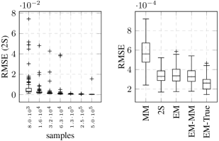
Figure 2: Each box contains 100 simulations. (Left) RMSE of the proposed algorithm at different data sizes. (Right) RMSE at $5\!\cdot\!10^{5}$ samples (one outlier not seen).

We sampled observations from randomly generated systems of size $X=Y=5$. Notice that there are a total of 20 unknown parameters (i.e., elements of $P$) to estimate for such systems. We used an elementwise lower bound $\underaccent{\bar}{\Pi}$ of one tenth of the minimum element of the true stationary distribution of each system. We compared the performance of the proposed two-step algorithm (2S), to the estimate resulting from the method of moments (MM), as well as, the EM algorithm started in three different initial points: a random point (EM), the method of moments estimate (EM-MM) and the true parameter values (EM-True).

Fig. 1 presents the median over 100 simulations for each batch size of, left, the root mean squared error (RMSE) and, right, the run-time. Fig. 2 presents box plots of, left, the RMSEs of the proposed algorithm at various data sizes and, right, the RMSEs of the compared algorithms for $5\cdot 10^{5}$ samples. All boxes contain 100 simulations. Three things can be noted from the figures.

Firstly, in the left plot of Fig. 1, the loss of accuracy resulting from only using the second order moments (compared to all moments in EM) is apparent from the distance between the MM-curve and the EM-curves. This can also be seen in the right plot of Fig. 2.

Secondly, also in the left plot of Fig. 1, we see that the asymptotics become valid around $10^{5}$ samples which takes the estimate resulting from the proposed two-step method down to the accuracy of EM. The same conclusion is indicated by the left plot of Fig. 2, where the number of observed outliers drop. These occurred when the Hessian was not negative definite – a result of the initial estimate not being sufficiently close to the maximum of the likelihood function. Note that this can be detected prior to employing the method.

Thirdly, in the right plot of Fig. 1, it can be see that the run-times of the compared algorithms differ by up to an order of magnitude. It should moreover be noted that the run-time of the proposed algorithm is more or less constant for a fixed data size (i.e., independent of the system and the observations), whereas the run-time of EM is highly dependent on the data (due to the number of iterations needed to converge): The maximum run-times for $5\cdot 10^{5}$ observations were 1083, 480, 166 seconds for EM, EM-MM and EM-True, respectively, whereas for the proposed method it was 54 seconds.

VI Conclusion

This letter has proposed and analyzed a two-step algorithm for identification of HMMs with known sensor uncertainties. A method of moments was combined with direct likelihood maximization to exploit the benefits of both approaches: lower computational cost and consistency in the former, and accuracy in the later. Theoretical guarantees were given for asymptotic efficiency and numerical simulations showed that the algorithm can yield the same accuracy as the standard EM algorithm, but in up to an order of magnitude less time.

Here, we provide details of the proofs stated in the paper.

Appendix A Proof of Lemma 1

To show the equivalence, we first establish that the mappings between $P$ and $\pi_{\infty}$, and $A$ are one-to-one using the following lemma.

Lemma 3.

The mappings (8), (9) and (10) between $P$ and $\pi_{\infty}$, and $A$ are one-to-one.

Proof.

Recall that $\pi_{\infty}$ has strictly positive elements. Firstly, given $P$ and $\pi_{\infty}$, the equation (8) yields a single $A$. Secondly, assume $\operatorname{diag}(\pi_{\infty})P=A=\operatorname{diag}(\tilde{\pi}_{\infty})\tilde{P}$, where $\tilde{P}$ and $P$ are row-stochastic. Multiplying the equation by $\mathds{1}$ from the right yields $\pi_{\infty}=\tilde{\pi}_{\infty}$. Then, multiplying from the left by $\operatorname{diag}(\pi_{\infty})^{-1}$ yields $P=\tilde{P}$.

Thirdly, equations (9) and (10) yield unique $P$ and $\pi_{\infty}$ given an $A$. Fourthly, assume $A$ and $\tilde{A}$ both map to $P$ and $\pi_{\infty}$, i.e., $A\mathds{1}=\pi_{\infty}=\tilde{A}\mathds{1}$, and $\operatorname{diag}(A\mathds{1})^{-1}A=P=\operatorname{diag}(\tilde{A}\mathds{1})^{-1}\tilde{A}$. Multiplying the last equation by $\operatorname{diag}(A\mathds{1})$ yields $A=\tilde{A}$. ∎

Then we note that the cost functions are the same in the two formulations (6) and (7) of the problem. Secondly, we map feasible solutions between the two problems.

A-1 Solution of (6) $\Rightarrow$ Solution of (7)

Assume $P$ and $\pi_{\infty}$ are optimal for (6), and define $A=\operatorname{diag}(\pi_{\infty})P$. Then

• $P\geq 0,\pi_{\infty}\geq 0\Rightarrow A\geq 0$,

• $\mathds{1}^{T}A\mathds{1}=\mathds{1}^{T}\operatorname{diag}(\pi_{\infty})P\mathds{1}=\pi_{\infty}^{T}\mathds{1}=1$,

• $A\mathds{1}=\operatorname{diag}(\pi_{\infty})P\mathds{1}=\operatorname{diag}(\pi_{\infty})\mathds{1}=\pi_{\infty}\in\underaccent{\bar}{\Pi}$,

• $\pi_{\infty}=P^{T}\pi_{\infty}\Rightarrow\operatorname{diag}(\pi_{\infty})\mathds{1}=P^{T}\operatorname{diag}(\pi_{\infty})\mathds{1}\overset{P\mathds{1}=\mathds{1}}{\Rightarrow}\operatorname{diag}(\pi_{\infty})P\mathds{1}=[\operatorname{diag}(\pi_{\infty})P]^{T}\mathds{1}\Rightarrow A\mathds{1}=A^{T}\mathds{1}$.

A-2 Solution of (7) $\Rightarrow$ Solution of (6)

Assume $A$ is optimal for (7). Let $\pi_{\infty}=A\mathds{1}$ and $P=\operatorname{diag}(A\mathds{1})^{-1}A$. Note that $\operatorname{diag}(A\mathds{1})^{-1}$ is well-defined since $A\mathds{1}\in\underaccent{\bar}{\Pi}$, i.e., $A\mathds{1}>0$. Then

• $A\geq 0\Rightarrow\pi_{\infty}\geq 0\text{ and }P\geq 0$,

• Since for any vector $x$ with all non-zero elements it holds that $[\operatorname{diag}(x)^{-1}x]_{i}=[\operatorname{diag}(x)^{-1}]_{ii}[x]_{i}=[x]_{i}^{-1}[x]_{i}=1$, i.e., $\operatorname{diag}(x)^{-1}x=\mathds{1}$, we have that $\mathds{1}=\operatorname{diag}(A\mathds{1})^{-1}A\mathds{1}=P\mathds{1}$,

• $\mathds{1}^{T}A\mathds{1}=1\Rightarrow\mathds{1}^{T}\pi_{\infty}=1$,

• $\pi_{\infty}=A\mathds{1}\in\underaccent{\bar}{\Pi}$,

• $A\mathds{1}=A^{T}\mathds{1}\Rightarrow\pi_{\infty}=A^{T}\mathds{1}$. Then, again employing that $\operatorname{diag}(x)^{-1}x=1$ for any vector with all non-zero elements; $\pi_{\infty}=A^{T}\mathds{1}=A^{T}\operatorname{diag}(A\mathds{1})^{-1}A\mathds{1}=[\operatorname{diag}(A\mathds{1})^{-1}A]^{T}A\mathds{1}=P^{T}\pi_{\infty}$.

Appendix B Proof of Lemma 2

Here, we provide a sequence of lemmas that give the details on that

1. the estimate $\hat{M}_{\infty}$ converges to $M_{\infty}$,

2. the solution $\hat{A}$ of the optimization problem (7) converges to the true parameter $A$,

3. the solution $\hat{A}$ of the optimization problem (7) can be converted uniquely to $\hat{P}$ and $\hat{\pi}_{\infty}$.

B-A Convergence of $\hat{M}_{\infty}$

Lemma 4.

Let the sequence of $N$ observations from the HMM with initial distribution $\pi_{0}$ be the set $\{y_{k}\}_{k=0}^{N}$ and form the empirical estimate (5) of the second order moments. Then the estimate converges, i.e.,

$$\hat{M}_{\infty}\rightarrow B^{T}\operatorname{diag}(\pi_{\infty})PB$$ (14)

with probability one as the number of observations $N\rightarrow\infty$.

Before we prove the above lemma, we first introduce two auxiliary lemmas.

Lemma 5.

Let $x_{k}$ be the state of an HMM and $y_{k}$ the corresponding observation. Then the process defined by the tuplet $(x_{k},y_{k},y_{k-1})$ is a Markov chain.

Proof.

It can be checked that the Markov property is satisfied. ∎

The above lemma allows us to recast the HMM into a Markov chain so that we can leverage convergence results related to Markov chains. The following lemma guarantees necessary properties of this new Markov chain:

Lemma 6.

If the transition and observation matrices of the HMM referred to in Lemma 5 have all elements strictly positive, then the Markov chain $(x_{k},y_{k},y_{k-1})$ is irreducible and aperiodic.

Proof.

The transition matrix of the lumped Markov chain consists of multiplications between elements of the $P$ and $B$ matrices (which are strictly positive) and zeros (whenever the common observation is not shared).

It can be shown that any state can reach any state with positive probability in at most two steps ($\Rightarrow$ irreducibility). Furthermore, it can be shown that any state with the same two observations has positive probability of returning to itself in one step ($\Rightarrow$ aperiodicity). ∎

With these two lemmas, we are now ready to prove Lemma 4.

Proof of Lemma 4.

Denote the state of the lumped Markov chain as $z_{k}=(y_{k},y_{k+1},x_{k+1})$ and let the functions $f_{ij}$ be given by

$$f_{ij}(z_{k})=\text{I}\{y_{k}=i,y_{k+1}=j\}.$$ (15)

Then,

$$\lim_{N\rightarrow\infty}[\hat{M}_{\infty}]_{ij} =\lim_{N\to\infty}\frac{1}{N}\sum_{k=0}^{N-1}\text{I}\{y_{k}=i,y_{k+1}=j\}$$

$$=\lim_{N\to\infty}\frac{1}{N}\sum_{k=0}^{N-1}f_{ij}(z_{k})$$

$$\rightarrow\sum_{z\in\mathcal{Z}}\tilde{\pi}_{\infty}(z)f_{ij}(z)$$

$$=\sum_{x\in\mathcal{X}}\tilde{\pi}_{\infty}((i,j,x))$$

$$=\sum_{x\in\mathcal{X}}\lim_{k\to\infty}\operatorname{Pr}[(y_{k},y_{k+1},x_{k+1})=(i,j,x)]$$

$$=\lim_{k\to\infty}\operatorname{Pr}[(y_{k},y_{k+1})=(i,j)]$$

$$=[B^{T}\operatorname{diag}(\pi_{\infty})PB]_{ij}$$

$$=[M_{\infty}]_{ij},$$

with probability one, where $\mathcal{Z}=\mathcal{Y}\times\mathcal{Y}\times\mathcal{X}$ and $\tilde{\pi}_{\infty}$ is the stationary distribution of $z_{k}$. Here, we used that $z_{k}$ is aperiodic and irreducible (Lemma 6) and the strong law of large numbers for Markov chains [5, Theorem 14.2.53]. ∎

B-B Convergence of optimization solution

As guaranteed by Lemma 4, the estimate $\hat{M}_{\infty}$ will converge to $M_{\infty}$ with probability one. The next step is to show that the solution(s) of the optimization problem (7) converges to the optimal value, i.e., that $\hat{A}\rightarrow A$, as $\hat{M}_{\infty}\rightarrow M_{\infty}$. The following lemma guarantees that there is a unique solution to the optimization problem and allows us to write the minimizer from here on.

Lemma 7.

Under the assumption that $B$ has full rank, the minimizer of the optimization problem (7) is unique.

Proof.

We check that the Hessian of the cost function in (7) is positive definite to ensure strict convexity (see, e.g., [31]). Note that the cost is of the form (see equation (34) below for details)

$$f(x) =\|Qx+q\|_{2}^{2}$$

$$=x^{T}Q^{T}Qx+2q^{T}Qx+q^{T}q,$$ (16)

where $Q=B^{T}\otimes B^{T}$, which has the Hessian

$$\nabla^{2}f(x)=2Q^{T}Q.$$ (17)

Positive definiteness of the Hessian is, in this case, equivalent to

$$x^{T}\big{[}\nabla^{2}f(x)\big{]}x>0 \quad\forall x\neq 0 \Leftrightarrow$$

$$x^{T}\big{[}2Q^{T}Q]x>0 \quad\forall x\neq 0 \Leftrightarrow$$

$$2(Qx)^{T}(Qx)>0 \quad\forall x\neq 0 \Leftrightarrow$$

$$2\|Qx\|^{2}>0 \quad\forall x\neq 0 \Leftrightarrow$$

$$Qx\neq 0 \quad\forall x\neq 0 \Leftrightarrow$$

$$\ker Q=\{0 \}.$$ (18)

Since (see, e.g., [32])

$$\operatorname{rank}(B^{T}\otimes B^{T})=\operatorname{rank}(B^{T})\operatorname{rank}(B^{T})=X^{2},$$ (19)

we see that the $Y^{2}\times X^{2}$ matrix $B^{T}\otimes B^{T}$ has full column rank. By (18), this implies uniqueness since, then, the cost function is strictly convex. ∎

The next lemma says that the sequence of minimizers of the approximate optimization problems will converge to the minimizer of the true optimization problem.

Lemma 8.

Let $\hat{A}$ be the minimizer of the optimization problem (7) using $\hat{M}_{\infty}$ from equation (5), and let $A$ be the minimizer of the optimization problem (7) using instead the true $M_{\infty}$. Then $\hat{A}$ converges with probability one to $A$ as $\hat{M}_{\infty}$ tends to $M_{\infty}$ as in Lemma 4.

To be able to prove Lemma 8, we will make use of another two additional lemmas. The first one provides results regarding how well a minimizer of an approximate cost function is with respect to the minimizer of the true cost function. In summary, it says that if we have uniform convergence of the cost function, the minimizer of the approximate cost function will converge to the minimizer of the true cost function, if the parameter set is compact.

Lemma 9.

Consider a family of random functions $f_{k}(\theta):\Theta\to\mathbb{R}$, where $\Theta$ is a compact subset of some Euclidean space. Let $\theta_{k}=\operatorname*{arg\,min}_{\theta\in\Theta}f_{k}(\theta)$. If $f_{k}(\theta)$ tends uniformly to a continuous (on $\Theta$) deterministic limit $\bar{f}(\theta)$ with probability one, i.e.,

$$\sup_{\theta\in\Theta}|f_{k}(\theta)-\bar{f}(\theta)|\to 0$$ (20)

with probability one as $k\to\infty$, then with $\Theta^{*}=\{\theta\in\Theta\text{ s.t. }\theta\text{ minimizes }\bar{f}(\theta)\}$, we have that

$$\inf_{\theta\in\Theta^{*}}\|\theta_{k}-\theta\|\to 0$$ (21)

with probability one as $k\to\infty$.

Proof.

This follows from Lemma 1.1 of [23] by restricting to the realizations where (20) hold. Similar results also appear in [33] and [34, Ch. 24]. ∎

The second auxiliary lemma needed states roughly that if we have pointwise convergence with probability one of a sequence of convex functions, then we also have uniform convergence over compact sets with probability one.

Lemma 10.

Suppose $f_{k}(\theta)$ is a sequence of convex random functions defined on an open convex set $\mathcal{S}$ of some Euclidean space, which converges pointwise in $\theta$ with probability one to some $\bar{f}(\theta)$. Then

$$\sup_{\theta\in\Theta}|f_{k}(\theta)-\bar{f}(\theta)|$$ (22)

tends to zero with probability one as $k\to\infty$, for each compact subset $\Theta$ of $\mathcal{S}$.

Proof.

This lemma follows from [24, Theorem 10.8] by restricting to the set of realizations where pointwise convergence holds, which has probability one by assumption. ∎

Combining these two lemmas allows us to provide proof for Lemma 8.

Proof of Lemma 8.

The cost function in problem (7) is strictly convex (see proof of Lemma 7). The set of feasible parameters is compact and convex. From Lemma 4, we know that $\hat{M}_{\infty}$ converges with probability one. Since the cost function is a continuous mapping of $\hat{M}_{\infty}$, we conclude that the cost function converges pointwise with probability one. Hence, the conditions of Lemma 10 are fulfilled. This in turn fulfills the conditions of Lemma 9 which allows us to conclude that $\hat{A}$ will tend to $A$ with probability one. ∎

B-C Convergence of $\hat{P}$ and $\hat{\pi}_{0}$

From Lemma 8, we know that $\hat{A}\rightarrow A$ as the number of samples tends to infinity. Since the mapping from $A$ to $P$ and $\pi_{\infty}$ is unique (see Lemma 3), we conclude that the estimates of $P$ and $\pi_{\infty}$ also will converge. In summary, this concludes the proof of Theorem 2.

Appendix C Proof of Theorem 1

Parts of the proof are inspired by [11].

C-1 Central limit theorem for $\hat{M}_{\infty}$

We will show that a central limit theorem holds for the estimates. For this, we employ the following theorem from [25]:

Theorem 2 (Corollary 5 of [25]).

Consider a uniformly ergodic Markov chain on $\mathcal{X}$ with stationary distribution $\pi_{\infty}$. Suppose $\mathbb{E}_{\pi_{\infty}}f^{2}(x)<\infty$, where $f:\mathcal{X}\to\mathbb{R}$. Then for any initial distribution, as $N\to\infty$,

$$\sqrt{N}(\bar{f}_{N}-\mathbb{E}_{\pi_{\infty}}f)\to_{d}\mathcal{N}(0,\sigma^{2}_{f}),$$ (23)

where $\bar{f}_{N}=N^{-1}\sum_{k=1}^{N}f(x_{k})$ and $\sigma_{f}^{2}<\infty$ is a constant.

As in the proof of Lemma 4, denote the state of the lumped Markov chain as $z_{k}=(y_{k},y_{k+1},x_{k+1})\in\mathcal{Z}=\mathcal{Y}\times\mathcal{Y}\times\mathcal{X}$ and let the functions $f_{ij}$ be given by

$$f_{ij}(z_{k})=\text{I}\{y_{k}=i,y_{k+1}=j\}.$$ (24)

Then, as guaranteed by Theorem 2 ($z_{k}$ is uniformly ergodic since it is finite – see [25, Example 1]),

$$\sqrt{N}\Bigg{(}\frac{1}{N}\sum_{k=0}^{N-1}f_{ij}(z_{k})-\sum_{z\in\mathcal{Z}}\tilde{\pi}_{\infty}(z)f_{ij}(z)\Bigg{)}\to_{d}\mathcal{N}(0,\sigma_{ij}^{2}),$$ (25)

or by changing back to the original variables,

$$\sqrt{N}\Bigg{(}\frac{1}{N} \sum_{k=0}^{N-1}\text{I}\{y_{k}=i,y_{k+1}=j\}$$

$$-\lim_{k\to\infty}\operatorname{Pr}[y_{k}=i,y_{k+1}=j]\Bigg{)}$$

$$\to_{d}\mathcal{N}(0,\sigma_{ij}^{2}),$$ (26)

i.e.,

$$\sqrt{N}\Big{(}[\hat{M}_{\infty}]_{ij}-[M_{\infty}]_{ij}\Big{)}\to_{d}\mathcal{N}(0,\sigma_{ij}^{2}),$$ (27)

where $\sigma_{ij}^{2}<\infty$ are constants.

C-2 $\sqrt{N}$-consistency of $\hat{M}_{\infty}$

We now establish that $\hat{M}_{\infty}$ is a $\sqrt{N}$-consistent estimator using the above result and the following lemma.

Lemma 11 (Appendix A, [26]).

If a sequence of random variables $Z_{N}$ and a constant $z_{0}$ tend in distribution to another random variable $Z$ (as $N\to\infty$) according to

$$\sqrt{N}(Z_{N}-z_{0})\to_{d}Z,$$ (28)

then

$$Z_{n}-z_{0}=\mathcal{O}_{p}(N^{-1/2}).$$ (29)

Leveraging the above lemma, we conclude that

$$[\hat{M}_{\infty}]_{ij}=[M_{\infty}]_{ij}+\mathcal{O}_{p}(N^{-1/2}).$$ (30)

This, by definition, means that for every $\varepsilon>0$, we can find a constant $c_{ij}(\varepsilon)$ such that for all $N$ sufficiently large,

$$\operatorname{Pr}\Big{[}\sqrt{N}\big{|}[\hat{M}_{\infty}]_{ij}-[M_{\infty}]_{ij}\big{|}>c_{ij}(\varepsilon)\Big{]}<\varepsilon.$$ (31)

C-3 $\sqrt{N}$-consistency of $\hat{A}$

We now propagate the $\sqrt{N}$-consistency of $\hat{M}_{\infty}$ to the variable $\hat{A}$ through the optimization problem (7).

First note that problem (7) can be rewritten on the standard form for a quadratic program (QP),

$$\min_{x}\quad \frac{1}{2}x^{T}Qx-q^{T}x$$

s.t. $$Gx\leq g,$$

$$Dx=d,$$ (32)

where $Q$ is a positive definite matrix. In particular, using the identity (for arbitrary matrices $A$, $B$ and $C$ of appropriate dimensions, see, e.g., [32])

$$\operatorname{vec}(ABC)=(C^{T}\otimes A)\operatorname{vec}(B),$$ (33)

we have that

$$\|\hat{M}_{\infty} -B^{T}AB\|_{F}^{2}=\|\operatorname{vec}(\hat{M}_{\infty}-B^{T}AB)\|_{2}^{2}$$

$$=\|\operatorname{vec}(\hat{M}_{\infty})-\operatorname{vec}(B^{T}AB)\|_{2}^{2}$$

$$=\|\operatorname{vec}(\hat{M}_{\infty})-(B\otimes B)^{T}\operatorname{vec}(A)\|_{2}^{2}$$

$$=\operatorname{vec}(\hat{M}_{\infty})^{T}\operatorname{vec}(\hat{M}_{\infty})$$

$$-2\operatorname{vec}(\hat{M}_{\infty})^{T}(B\otimes B)^{T}\operatorname{vec}(A)$$

$$+\operatorname{vec}(A)^{T}(B\otimes B)(B\otimes B)^{T}\operatorname{vec}(A),$$ (34)

so that,

$$Q =2(B\otimes B)(B\otimes B)^{T},$$ (35)

$$\hat{q} =2(B\otimes B)\operatorname{vec}(\hat{M}_{\infty}),$$ (36)

where $x=\operatorname{vec}(A)$, and the constant term has been dropped. The constraints can similarly be translated by vectorization, e.g., $\mathds{1}^{T}A\mathds{1}=1$ translates to $\mathds{1}^{T}\operatorname{vec}(A)=1$, i.e., $\mathds{1}^{T}x=1$.

The uncertainty in this problem, resulting from the estimation procedure, lies in the estimate of the moments $\hat{M}_{\infty}$. Note that this only influences the cost function – not the constraints. We now ask ourselves how the uncertainty in $\hat{M}_{\infty}$ propagates through the QP into our variable of interest $\hat{A}$.

Denote the minimizer of the nominal problem (32), where $M_{\infty}$ is used instead of $\hat{M}_{\infty}$, as $x^{*}$ (= $\operatorname{vec}(A)$) and let

$$\hat{x}^{*}=\operatorname*{arg\,min}_{x}\frac{1}{2}x^{T}Qx-\hat{q}^{T}x,$$ (37)

subject to the same constraints as in problem (32). Then [27, Theorem 2.1] provides the following bound on the distance between the solution of the nominal QP and the solution of the perturbed QP:

$$\|x^{*}-\hat{x}^{*}\|_{2}\leq\frac{\delta}{\lambda-\delta}(1+\|x^{*}\|_{2}),$$ (38)

where $\delta=\|q-\hat{q}\|_{2}$ and $\lambda$ is the smallest eigenvalue of $Q$.

Let $\sigma_{1}(\cdot)$ denote the largest singular value, then we note that (for every $\varepsilon>0$)

$$\delta =\|q-\hat{q}\|_{2}$$

$$=\|2(B\otimes B)\operatorname{vec}(M_{\infty})-2(B\otimes B)\operatorname{vec}(\hat{M}_{\infty})\|_{2}$$

$$=2\,\|(B\otimes B)(\operatorname{vec}(M_{\infty})-\operatorname{vec}(\hat{M}_{\infty}))\|_{2}$$

$$\leq 2\,\sigma_{1}(B\otimes B)\;\|\operatorname{vec}(M_{\infty})-\operatorname{vec}(\hat{M}_{\infty})\|_{2}$$

$$\leq 2\,\sigma_{1}(B\otimes B)\;\|\operatorname{vec}(M_{\infty})-\operatorname{vec}(\hat{M}_{\infty})\|_{1}$$

$$=2\,\sigma_{1}(B\otimes B)\;\sum_{i,j\in\mathcal{Y}}\big{|}[M_{\infty}]_{ij}-[\hat{M}_{\infty}]_{ij}\big{|}$$

$$\leq 2\,\sigma_{1}(B\otimes B)\;\sum_{i,j\in\mathcal{Y}}\frac{c_{ij}(\varepsilon)}{\sqrt{N}}$$

$$\leq\frac{1}{\sqrt{N}}\;2\,\sigma_{1}(B\otimes B)\;Y^{2}\max_{i,j}c_{ij}(\varepsilon)$$

$$\overset{\text{def.}}{=}\frac{1}{\sqrt{N}}\;K(\varepsilon),$$ (39)

with probability greater than $1-\varepsilon$, where $c_{ij}(\varepsilon)$ are the constants in the stochastic order (30). Also note that

$$\|x^{*}\|_{2}=\|\operatorname{vec}(A)\|_{2}\leq\|\mathds{1}_{X^{2}}\|_{2}=\sqrt{X^{2}}=X,$$ (40)

due to the sum-to-one constraint of $A$.

Hence, for every $\varepsilon>0$ (and $N$ sufficiently large), we have in the bound (38), that

$$\|A-\hat{A}\|_{F} =\|\operatorname{vec}(A)-\operatorname{vec}(\hat{A})\|_{2}$$

$$=\|x^{*}-\hat{x}^{*}\|_{2}$$

$$\leq\frac{\delta}{\lambda-\delta}(1+\|x^{*}\|_{2})$$

$$\leq\frac{\delta}{\lambda}\;(1+\|x^{*}\|_{2})$$

$$\leq\frac{1}{\sqrt{N}}\;\frac{K(\varepsilon)\;(1+X)}{\lambda}$$ (41)

with probability greater than $1-\varepsilon$. This shows that

$$\hat{A}=A+\mathcal{O}_{p}(N^{-1/2}).$$ (42)

C-4 $\sqrt{N}$-consistency of $\hat{\pi}_{\infty}$ and $\hat{P}$

Again, for any $\varepsilon>0$, we have using equation (9) that

$$\|\pi_{\infty}-\hat{\pi}_{\infty}\|_{2} =\|A\mathds{1}-\hat{A}\mathds{1}\|_{2}$$

$$=\|(A-\hat{A})\mathds{1}\|_{2}$$

$$\leq\Big{(}\max_{\|y\|_{2}=1}\|(A-\hat{A})y\|_{2}\Big{)}\|\mathds{1}\|_{2}$$

$$\leq\|A-\hat{A}\|_{F}\|\mathds{1}\|_{2}$$

$$=\|A-\hat{A}\|_{F}\sqrt{X}$$

$$\leq\frac{1}{\sqrt{N}}\;\frac{K(\varepsilon)\;(1+X)\sqrt{X}}{\lambda}$$ (43)

holds with probability greater than $1-\varepsilon$.

Continuing, equations (9) and (10) tell us that

$$\|P-\hat{P}\|_{F}=\|\operatorname{diag}(A\mathds{1})^{-1}A-\operatorname{diag}(\hat{A}\mathds{1})^{-1}\hat{A}\|_{F}.$$ (44)

We will use that, for two invertible diagonal matrices $D_{1}$ and $D_{2}$, and arbitrary matrices $X$ and $Y$, it holds that

$$\|D_{1}^{-1}X -D_{2}^{-1}Y\|_{F}=\|D_{1}^{-1}D_{2}^{-1}(D_{2}X-D_{1}Y)\|_{F}$$

$$\leq\|D_{1}^{-1}D_{2}^{-1}\|_{F}\|D_{2}X-D_{1}Y\|_{F}$$

$$\leq\|D_{1}^{-1}\|_{F}\|D_{2}^{-1}\|_{F}\|D_{2}X-D_{1}Y+D_{1}X-D_{1}X\|_{F}$$

$$=\|D_{1}^{-1}\|_{F}\|D_{2}^{-1}\|_{F}\|(D_{2}-D_{1})X+D_{1}(X-Y)\|_{F}$$

$$\leq\|D_{1}^{-1}\|_{F}\|D_{2}^{-1}\|_{F}$$

$$\quad\quad\times\Big{(}\|D_{2}-D_{1}\|_{F}\|X\|_{F}+\|D_{1}\|_{F}\|X-Y\|_{F}\Big{)}.$$ (45)

This yields

$$\|P-\hat{P}\|_{F}\leq\| \operatorname{diag}(A\mathds{1})^{-1}\|_{F}\|\operatorname{diag}(\hat{A}\mathds{1})^{-1}\|_{F}$$

$$\times\Big{(}\|\hat{A}\mathds{1}-A\mathds{1}\|_{2}\|A\|_{F}+\|A\mathds{1}\|_{2}\|A-\hat{A}\|_{F}\Big{)},$$ (46)

where the first factor is bounded by a constant due to the ergodicity assumptions (the stationary distribution has strictly positive elements) and the terms in the parenthesis have trivial bounds, or can be bounded using equations (41) and (43). Hence, for any $\varepsilon>0$, we have that $\|P-\hat{P}\|_{F}\leq\frac{\text{constant}}{\sqrt{N}}$ with probability greater than $1-\varepsilon$, or equivalently that,

$$\hat{P}=P+\mathcal{O}_{p}(N^{-1/2}).$$ (47)

C-5 $\Delta$-method

Assume that the parametrization of the transition matrix is continuous and differentiable, and denote by $\theta^{*}$ the true parameters. We can then propagate relation (47) to the parameters $\theta$ to obtain

$$\hat{\theta}_{\text{MM}}=\theta^{*}+\mathcal{O}_{p}(N^{-1/2}),$$ (48)

using the $\Delta$-method – in particular, the first part of the proof of Theorem 3.1 in [35].

C-6 Regularity of the likelihood function

Denote the Fisher information matrix as $I_{F}(\theta^{*})$. Then Theorems 12.5.5 and 12.5.6 of [5] guarantee that we have a central limit theorem for the score function and a law of large numbers for the observed information matrix, as follows:

$$N^{-1/2}\nabla_{\theta}l_{N}(\theta^{*}) \rightarrow_{d}\mathcal{N}(0,I_{F}(\theta^{*}),$$ (49)

$$N^{-1}\nabla_{\theta}^{2}l_{N}(\theta^{*}) \rightarrow_{p}-I_{F}(\theta^{*}),$$ (50)

as $N\rightarrow\infty$, since our chain is finite and $P,B>0$.

C-7 Asymptotic efficiency by Newton-Raphson

Lemma 12.

Let $\hat{\theta}_{\text{init}}=\theta^{*}+\mathcal{O}_{p}(N^{-1/2})$. Then, one Newton-Raphson step starting in $\hat{\theta}_{\text{init}}$ on $l_{N}(\theta)$ gives an asymptotically efficient estimator, i.e., with

$$\hat{\theta}_{\text{NR}}=\hat{\theta}_{\text{init}}-\big{[}\nabla_{\theta}^{2}l_{N}(\hat{\theta}_{\text{init}})\big{]}^{-1}\;\nabla_{\theta}l_{N}(\hat{\theta}_{\text{init}}),$$ (51)

we get

$$\sqrt{N}(\hat{\theta}_{\text{NR}}-\theta^{*})\rightarrow_{d}\mathcal{N}(0,I_{F}^{-1}(\theta^{*})).$$ (52)

(Proof on next page)

Proof.

We have that

$$\sqrt{N}(\hat{\theta}_{\text{NR}}-\theta^{*}) =\sqrt{N}(\hat{\theta}_{\text{init}}-\theta^{*})-\sqrt{N}\big{[}\nabla_{\theta}^{2}l_{N}(\hat{\theta}_{\text{init}})\big{]}^{-1}\nabla_{\theta}l_{N}(\hat{\theta}_{\text{init}})$$

$$=\sqrt{N}(\hat{\theta}_{\text{init}}-\theta^{*})-N^{-1/2}\big{[}-I_{F}(\theta^{*})+o_{\text{p}}(1)\big{]}^{-1}\big{[}\nabla_{\theta}l_{N}(\theta^{*})+\nabla_{\theta}^{2}l_{N}(\theta^{*})(\hat{\theta}_{\text{init}}-\theta^{*})+o_{\text{p}}(1)\big{]}$$

$$=\sqrt{N}(\hat{\theta}_{\text{init}}-\theta^{*})-\big{[}-I_{F}(\theta^{*})+o_{\text{p}}(1)\big{]}^{-1}\Big{[}N^{-1/2}\nabla_{\theta}l_{N}(\theta^{*})+\sqrt{N}[-I_{F}(\theta^{*})+o_{\text{p}}(1)](\hat{\theta}_{\text{init}}-\theta^{*})+o_{\text{p}}(1)\Big{]}$$

$$=\sqrt{N}(\hat{\theta}_{\text{init}}-\theta^{*})+I_{F}^{-1}(\theta^{*})\Big{[}N^{-1/2}\nabla_{\theta}l_{N}(\theta^{*})-I_{F}(\theta^{*})\sqrt{N}(\hat{\theta}_{\text{init}}-\theta^{*})\Big{]}+o_{\text{p}}(1)$$

$$=I_{F}^{-1}(\theta^{*})N^{-1/2}\nabla_{\theta}l_{N}(\theta^{*})+o_{\text{p}}(1)$$

$$\to_{d}\mathcal{N}(0,I_{F}^{-1}(\theta^{*})I_{F}(\theta^{*})I_{F}^{-T}(\theta^{*})$$

$$=\mathcal{N}(0,I_{F}^{-1}(\theta^{*}).$$ (53)

∎

Lemma 52, together with the results of subsections C-4 and C-6, conclude the proof of Theorem 1 by taking $\hat{\theta}_{\text{init}}=\hat{\theta}_{MM}$.

References

- [1] V. Krishnamurthy, Partially Observed Markov Decision Processes. Cambridge University Press, 2016.
- [2] R. Durbin, Ed., Biological sequence analysis: Probabalistic models of proteins and nucleic acids. Cambridge University Press, 1998.
- [3] M. Vidyasagar, Hidden Markov Processes: Theory and Applications to Biology. Princeton University Press, 2014.
- [4] L. Rabiner, “A tutorial on hidden Markov models and selected applications in speech recognition,” Proceedings of the IEEE, vol. 77, no. 2, pp. 257–286, Feb. 1989.
- [5] O. Cappé, E. Moulines, and T. Rydén, Inference in Hidden Markov Models. Springer, 2005.
- [6] A. P. Dempster, N. M. Laird, and D. B. Rubin, “Maximum likelihood from incomplete data via the EM algorithm,” Journal of the Royal Statistical Society. Series B (Methodological), vol. 39, pp. 1–38, 1977.
- [7] S. M. Kay, Fundamentals of Statistical Signal Processing: Estimation Theory. Upper Saddle River, NJ, USA: Prentice-Hall, Inc., 1993.
- [8] B. Lakshminarayanan and R. Raich, “Non-negative matrix factorization for parameter estimation in hidden Markov models,” in Proceedings of the IEEE International Workshop on Machine Learning for Signal Processing (MLSP’10), 2010, pp. 89–94.
- [9] A. Anandkumar, D. Hsu, and S. M. Kakade, “A method of moments for mixture models and hidden Markov models,” in Proceedings of the 25th Conference on Learning Theory (COLT’12), 2012, pp. 33.1–33.34.
- [10] D. Hsu, S. M. Kakade, and T. Zhang, “A spectral algorithm for learning hidden Markov models,” Journal of Computer and System Sciences, vol. 78, no. 5, pp. 1460–1480, Sep. 2012.
- [11] A. Kontorovich, B. Nadler, and R. Weiss, “On learning parametric-output HMMs,” in Proceedings of the 30th International Conference on Machine Learning (ICML’13), vol. 28, 2013, pp. 702–710.
- [12] A. Anandkumar, R. Ge, D. Hsu, S. M. Kakade, and M. Telgarsky, “Tensor decompositions for learning latent variable models,” Journal of Machine Learning Research, vol. 15, no. 1, pp. 2773–2832, 2014.
- [13] R. Mattila, V. Krishnamurthy, and B. Wahlberg, “Recursive identification of chain dynamics in hidden Markov models using non-negative matrix factorization,” in Proceedings of the 54th IEEE Conference on Decision and Control (CDC’15), 2015, pp. 4011–4016.
- [14] Y. C. Subakan, J. Traa, P. Smaragdis, and D. Hsu, “Method of moments learning for left-to-right hidden Markov models,” in Proceedings of the IEEE Workshop on Applications of Signal Processing to Audio and Acoustics (WASPAA’15), 2015, pp. 1–5.
- [15] I. Meilijson, “A fast improvement to the EM algorithm on its own terms,” Journal of the Royal Statistical Society. Series B (Methodological), pp. 127–138, 1989.
- [16] J. A. Fessler and A. O. Hero, “Space-alternating generalized expectation-maximization algorithm,” IEEE Transactions on Signal Processing, vol. 42, no. 10, pp. 2664–2677, 1994.
- [17] T. C. Lystig and J. P. Hughes, “Exact computation of the observed information matrix for hidden Markov models,” Journal of Computational and Graphical Statistics, vol. 11, no. 3, pp. 678–689, Sep. 2002.
- [18] O. Cappé and E. Moulines, “Recursive computation of the score and observed information matrix in hidden Markov models,” in Proceedings of the 13th IEEE Workshop on Statistical Signal Processing, 2005, pp. 703–708.
- [19] R. Turner, “Direct maximization of the likelihood of a hidden Markov model,” Computational Statistics & Data Analysis, vol. 52, no. 9, pp. 4147–4160, May 2008.
- [20] W. Khreich, E. Granger, A. Miri, and R. Sabourin, “A survey of techniques for incremental learning of HMM parameters,” Information Sciences, vol. 197, pp. 105–130, Aug. 2012.
- [21] I. L. MacDonald, “Numerical maximisation of likelihood: A neglected alternative to EM?” International Statistical Review, vol. 82, no. 2, pp. 296–308, Aug. 2014.
- [22] P.-J. Courtois and P. Semal, “On polyhedra of Perron-Frobenius eigenvectors,” Linear algebra and its applications, vol. 65, pp. 157–170, 1985.
- [23] M. Campi, “System identification and the limits of learning from data,” 2006. [Online]. Available: http://marco-campi.unibs.it/pdf-pszip/sys-id-and-limits-learning.pdf
- [24] R. T. Rockafellar, Convex Analysis. Princeton University Press, 1970.
- [25] G. L. Jones, “On the Markov chain central limit theorem,” Probability Surveys, vol. 1, pp. 299–320, 2004.
- [26] D. Pollard, Convergence of Stochastic Processes. Springer, 1984.
- [27] J. W. Daniel, “Stability of the solution of definite quadratic programs,” Mathematical Programming, vol. 5, no. 1, pp. 41–53, 1973.
- [28] M. Grant and S. Boyd, “CVX: Matlab software for disciplined convex programming, version 2.1,” http://cvxr.com/cvx, Mar. 2014.
- [29] A. Griewank and A. Walther, Evaluating Derivatives: Principles and Techniques of Algorithmic Differentiation, 2nd ed. Philadelphia, PA, USA: Society for Industrial and Applied Mathematics, 2008.
- [30] J. Revels, M. Lubin, and T. Papamarkou, “Forward-mode automatic differentiation in Julia,” arXiv:1607.07892 [cs.MS], 2016. [Online]. Available: https://arxiv.org/abs/1607.07892
- [31] S. Boyd and L. Vandenberghe, Convex Optimization. New York, NY: Cambridge University Press, 2004.
- [32] R. A. Horn and C. R. Johnson, Topics in matrix analysis. Cambridge University Press, 1991.
- [33] N. L. Hjort and D. Pollard, “Asymptotics for minimisers of convex processes,” Tech. Rep., 1993.
- [34] C. Gourieroux and A. Monfort, Statistics and Econometric Models. Cambridge University Press, 1995, vol. 2.
- [35] A. W. v. d. Vaart, Asymptotic Statistics. Cambridge University Press, 1998.