An analytical model for a full wind turbine wake

Abstract

An analytical wind turbine wake model is proposed to predict the wind velocity distribution for all distances downwind of a wind turbine, including the near-wake. This wake model augments the Jensen model and subsequent derivations thereof, and is a direct generalization of that recently proposed by Bastankhah and Porté-Agel. The model is derived by applying conservation of mass and momentum in the context of actuator disk theory, and assuming a distribution of the double-Gaussian type for the velocity deficit in the wake. The physical solutions are obtained by appropriate mixing of the waked- and freestream velocity deficit solutions, reflecting the fact that only a portion of the fluid particles passing through the rotor disk will interact with a blade.

1 Introduction

An analytical wind turbine wake model is proposed to predict the wind velocity distribution for all distances downwind of a wind turbine, including the near-wake. The model is derived by applying conservation of mass and momentum in the context of actuator disk theory, and assuming a distribution of the double-Gaussian-type for the velocity deficit in the wake.

In 1983 Jensen [1] proposed the first analytical model for a wind turbine wake. This model has become the de facto industry standard, and has been developed further by Fransden et al.[2] and more recently by Bastankhah and Porté-Agel [3]. These wake models are based upon mass and momentum conservation, and either a top-hat distribution [1], [2], or a Gaussian distribution [3] for the velocity deficit. The Ainslie model [4] is based on a numerical solution of the Navier-Stokes equations and uses a Gaussian near-wake approach. The model proposed by Larsen [5], [6] is based on the Prandtl turbulent boundary layer equations. The UPMWAKE model [7] is a Navier-Stokes code for the far wake based on a turbulence model. Magnusson [8] uses momentum theory and blade element theory, along with Prandtl’s approximation, to provide a numerical model for the near-wake. Some of the wake models mentioned have been integrated into wind farm design software.

This work is motivated by the desire to produce a model that more accurately predicts the near-wake region. The Jensen model provides a reasonable representation of the wake for the mid- and far-wake regimes, but there is a clear discrepancy in the near-wake, with the Jensen model predicting an unphysical drop-off in the centreline wake wind velocity, see for example references [9], [10], [11]. It is well known that the transverse velocity deficit profile can be represented by a single-Gaussian function for the mid- and far- wakes, but that in the near-wake the profile resembles a double-Gaussian function, with local minima at about 75$\%$ blade span [12], [13]. Thus, it is reasonable to consider a double-Gaussian function as a candidate for the transverse velocity deficit profile. However, this in itself is not sufficient to generate physically realistic solutions. These are obtained by subsequent, appropriate mixing of a wake velocity deficit solution and the freestream velocity. It is natural that such an adjustment should be required as only a fraction of the wind flow fluid particles passing through the rotor disk are affected by the blades [14], and the amount by which they are affected depends upon the pitch angle of the rotor blades. The double-Gaussian velocity deficit and the mixing of solutions are not part of the basic actuator disk scenario. Consideration is given only to wind turbine wakes in zero yaw situations. The predictions of this simple model are compared to real-scale wind turbine wake measurements.

According to blade element momentum theory, the axial flow induction factor varies radially and azimuthally across the rotor disk [14]. Here, for a particular wind flow regime, and in accordance with the actuator disk theory, a single value of axial flow induction factor shall be taken to be representative of the wind flow at the rotor disk. The proposed wake model is axially symmetric about the rotor axis. Inclusion of wind shear will be dealt with in a subsequent work.

The new wake model is derived in section 2. In section 3 the model is compared to wake measurements and estimates of quality of the fit are made. A comparison is also made with the Jensen model. An overview of the results is given in section 5.

2 Wake model derivation

The technique presented in Bastankhah and Porté-Agel [3] shall be followed closely.

2.1 Velocity deficit

Consideration is given only to wakes in zero yaw situations: All velocities are assumed to be in the axial direction. In the following $U_{\infty}$ shall denote the incoming wind velocity (the freestream velocity), $U$ is the wake velocity in the streamwise direction, and $U_{D}$ the velocity at the rotor disk. The normalized velocity deficit is defined as

$${\Delta U\over U_{\infty}}={(U_{\infty}-U)\over U_{\infty}}.$$ (1)

The axial flow induction factor is defined as [14]

$$a=1-{U_{D}\over U_{\infty}}.$$ (2)

The corresponding (theoretical) thrust coefficient for a wind turbine is defined as [14]

$$C_{T}=4a(1-a)$$ (3)

although an alternative empirical relationship between $C_{T}$ and $a$ can also be assumed, as described in chapter 4 of [14].

The velocity deficit is taken to be of the form

$${\Delta U\over U_{\infty}}=C(x)f(r,\sigma(x))$$ (4)

where $C(x)$ is an arbitrary function of downwind distance $x$, and $f$ is an arbitrary function of the radial distance from the rotor axis $r$ and $\sigma$, the wake cross-section at downwind distance $x$.

The double-Gaussian profile is given by

$$f(r,\sigma(x))=\case{1}{2}[\exp D_{+}+\exp D_{-}],\qquad D_{\pm}=-\case{1}{2}\sigma^{-2}(x)(r\pm r_{0})^{2}$$ (5)

where $r_{0}$ is the radius corresponding to the locii of the Gaussian minima and $\sigma(x)$ is a cross-section function. As expected, in the case where $r_{0}=0$, the above coincides with (12) in [3], i.e.,

$$f(r,\sigma(x))=\exp[-\case{1}{2}\sigma^{-2}(x)r^{2}].$$ (6)

2.2 Momentum conservation

The equation of mean momentum flux through the rotor disk plane (Equation (4.1.26) of Tennekes and Lumley [15]) is

$$\rho\int U(U_{\infty}-U)dA=T$$ (7)

where $\rho$ is the density of the air, $A$ is the cross-sectional area in the plane of the rotor blade motion, and $T$ is the total force over the wind turbine, given by

$$T=\frac{1}{2}C_{T}\rho A_{0}U^{2}_{\infty}.$$ (8)

The quantity $C_{T}$ is the thrust coefficient defined above, and $A_{0}$ is the area swept out by the turbine rotors, i.e., $A_{0}=\pi d^{2}_{0}/4$ where $d_{0}$ is the wind turbine rotor diameter.

Following a similar procedure to that given in [3], equation (7) is integrated. The integration is performed over the entire rotor disk plane, i.e., a disk of infinite radius $r$. The area $A=\pi r^{2}$ and it follows that

$$dA=2\pi rdr.$$ (9)

Thus, in order to evaluate equation (7), one must calculate the value of the integral

$$I=\int^{r=\infty}_{r=0}U(U_{\infty}-U)dA.$$ (10)

The ansatz for the velocity deficit will now be used to obtain solutions of equation (7).

2.3 Integration of equation of mean momentum flux

The explicit expression for this integral is

$$I=\pi\int^{r=\infty}_{r=0}U^{2}_{\infty}C(x)\biggl{(}\exp D_{+}+\exp D_{-}-\case{1}{2}C(x)Hrdr\biggr{)}$$ (11)

where

$$H=\exp(2D_{+})+\exp(2D_{-})+2\exp(D_{+}+D_{-}).$$ (12)

Upon integration this becomes (see Appendix)

$$I=\pi U^{2}_{\infty}C(x)[M-\case{1}{2}C(x)N]$$ (13)

where

$$M =2\sigma^{2}\exp(-\case{1}{2}\tau^{2})+\sqrt{2\pi}r_{0}\sigma[\mathrm{erfc}(\tau/\sqrt{2})-1]$$

$$N =\sigma^{2}\exp(-\tau^{2})+\case{1}{2}\sqrt{\pi}r_{0}\sigma[\mathrm{erfc}(\tau)-1]$$

$$\tau =r_{0}\sigma^{-1}.$$ (14)

Hence, equation (7) is

$$C^{2}(x)N-C(x)M+\case{1}{8}C_{T}d^{2}_{0}=0$$ (15)

whose solution is

$$C_{\pm}(x)={M\pm\sqrt{M^{2}-\case{1}{2}NC_{T}d^{2}_{0}}\over 2N}$$ (16)

The solution of equation (7) is given in terms of a Gaussian-type velocity deficit, with cross-section $\sigma$ chosen as

$$\sigma=k^{*}x^{n}+\epsilon$$ (17)

where $k^{*}$ and $\epsilon$ are constants and $n$ is an appropriately chosen exponent, see [2], [3], [15]. Classical theories of shear flows predict $n=1/3$ [15] and this value shall be adopted here. Note that $\sigma$ is the cross-section width of the single-Gaussian, rather than the cross-section of the full double-Gaussian. The velocity solutions $U_{\pm}$ of equation (7) are

$$U_{\pm}=U_{\infty}\biggl{(}1-C_{\pm}(x)f(r,\sigma(x))\biggr{)}.$$ (18)

One can carry out analysis in terms of the new dimensionless variable

$$X=\sigma/r_{0}.$$ (19)

In that case one can define and the solutions (16) can be expressed as

$${\cal C}_{\pm}(X)={{\cal M}\pm\sqrt{{\cal M}^{2}-\case{1}{2}{\cal N}C_{T}d^{2}_{0}r^{-2}_{0}}\over 2{\cal N}}.$$ (21)

The corresponding velocity solutions $U_{\pm}(X)$ are plotted for representative values of the thrust coefficient $C_{T}$ in Figure 1. Here and throughout, $r_{0}$ is taken to be 75$\%$ blade span in accordance with the empirical measurements in references [12] and [13], i.e., $r_{0}=0.75d_{0}/2$. The following facts are noted,

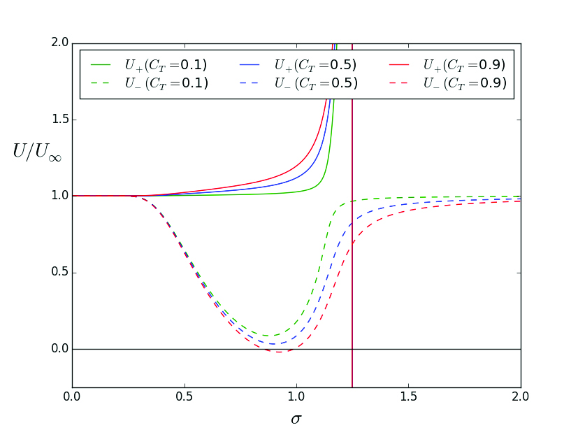
Figure 1: Wake centreline hub height horizontal normalized velocity profiles for the mean momentum flux equation solutions $U_{+}$ and $U_{-}$, for a selection of values of thrust coefficient $C_{T}$. The abscissa is the cross-section $\sigma$. The $U_{+}$ and $U_{-}$ solutions are represented by solid and dashed lines respectively. The $U_{-}$ solutions have local minima with values of approximately 0.1, 0.05 and -0.05 for $C_{T}$ values $0.1$, $0.5$ and $0.9$ respectively.

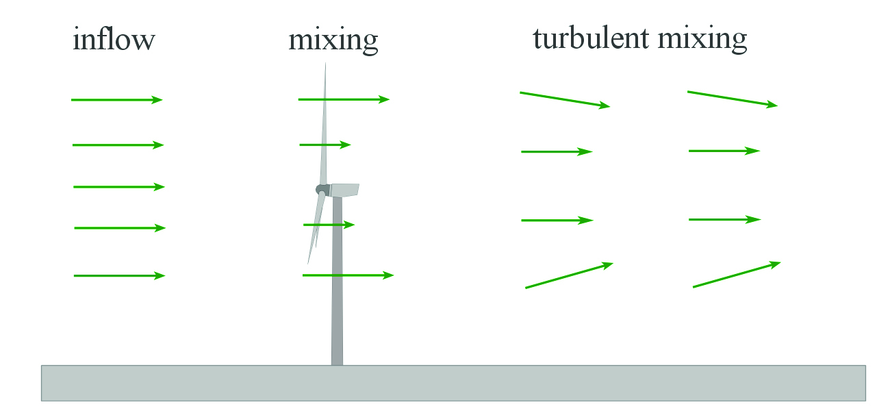
Figure 2: The mixing at the rotor and near wake of the wind turbine is governed by equation (22) and is distinct from the lateral turbulent mixing that occurs further downstream.

1. The $U_{+}$ solutions are unphysical.

2. The $U_{-}$ solutions show a clear local minimum for all non-zero values of $C_{T}$.

3. The $U_{-}$ solutions have the desired topological features, but the values of wake velocity at the local minima of the $U_{-}$ solutions are far lower than those obtained from empirical measurements.

4. The ambient background velocity (freestream velocity) $U_{\infty}$ is a (trivial) solution of the equation of mean momentum flux (7) for $T=0$.

The key to reconciling the above theory with the true measured wake velocity profiles is to consider a linear combination of solutions (mixing).

2.4 Velocity deficit solution: Mixing in the wake

Motivated by the facts i - iv noted above, it is conjectured that the real velocity solution in the wake is a linear combination of the solution $U_{-}$ and the freestream velocity $U_{\infty}$, as depicted in Figure 2. This real solution is

$$U=c_{-}U_{-}+c_{\infty}U_{\infty},\qquad c_{-}+c_{\infty}=1$$ (22)

for constants $c_{-}$ and $c_{\infty}$. Both solutions $U_{-}$ and $U_{\infty}$ are present in the wake, the combination of the two states through mixing gives rise to the final wind velocity profile. It is noted that a $c_{+}U_{+}$ term is not included because the resultant solutions $U$ will always be unphysical. The following points are noted.

1. The equation of mean momentum flux together with the actuator disk theory provide one component of the solution ($U_{-}$). It is conjectured that this represents the component actually affected by the rotor blades.

2. The other component is provided by the trivial solution, i.e. the solution had there been no wind turbine, namely that corresponding to the ambient background velocity (freestream velocity) $U_{\infty}$.

The constant $c_{-}$, and hence $c_{\infty}$, will vary with $C_{T}$. Recall that in the case of high wind velocity ($U_{\infty}\gtrsim 12m/s$) a relatively low proportion of energy is being extracted from the wind since the blades are in pitch/stall mode. In that case $c_{-}$ will be relatively small and $c_{\infty}$ relatively large. In the low $U_{\infty}$ regime $c_{-}$ will be relatively large.

As stated in section 3.8 of [14], much of the theory and analysis in the literature is based on the assumption that there is a sufficient number of blades in the rotor disk for every fluid particle in the rotor disk to interact with a blade. However, with a small number of blades most fluid particles will pass between the blades and the loss of momentum by a fluid particle will depend upon its proximity to a blade. Further, close to the blade tips, the tip vortex causes very high values of $a$ such that, locally, the net flow past the blade is in the upstream direction. These facts are qualitatively consistent with the proposed model and give credence to the method of construction of solutions above and their interpretation.

Figure 3 shows the wind velocity for the hub height horizontal section through the wake model, and the corresponding radial wind velocity, as would be measured by a nacelle-mounted LiDAR. Worthy of note is the “jet structure” in the near-wake, with local minima at about 75$\%$ blade span [12], [13], arising from the double-Gaussian wind velocity deficit distribution. The model exhibits the characteristic wake expansion downwind of the turbine rotor.

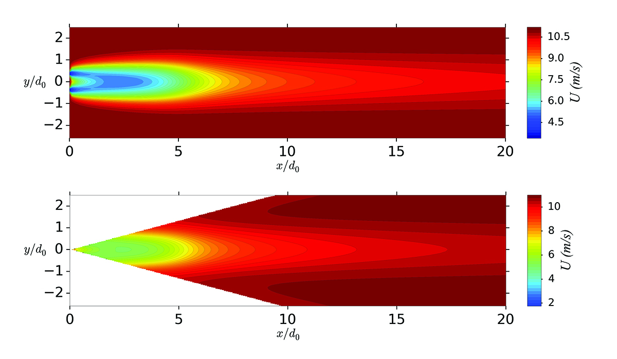
Figure 3: The top plot shows the wind velocity for the hub height horizontal section through the wake model. The lower plot shows the corresponding radial wind velocity, as would be measured by a nacelle-mounted LiDAR with $30^{\circ}$ horizontal scanning arc. $U_{\infty}=11ms^{-1}$.

Figure 4 shows the wind velocity profiles for the hub height horizontal cross-sections through the wake model, for $U_{\infty}=11ms^{-1}$, for various downwind distances. It is clear that there is a transition from double-Gaussian to single-Gaussian distribution at a downwind distance of about $2.5d_{0}$.

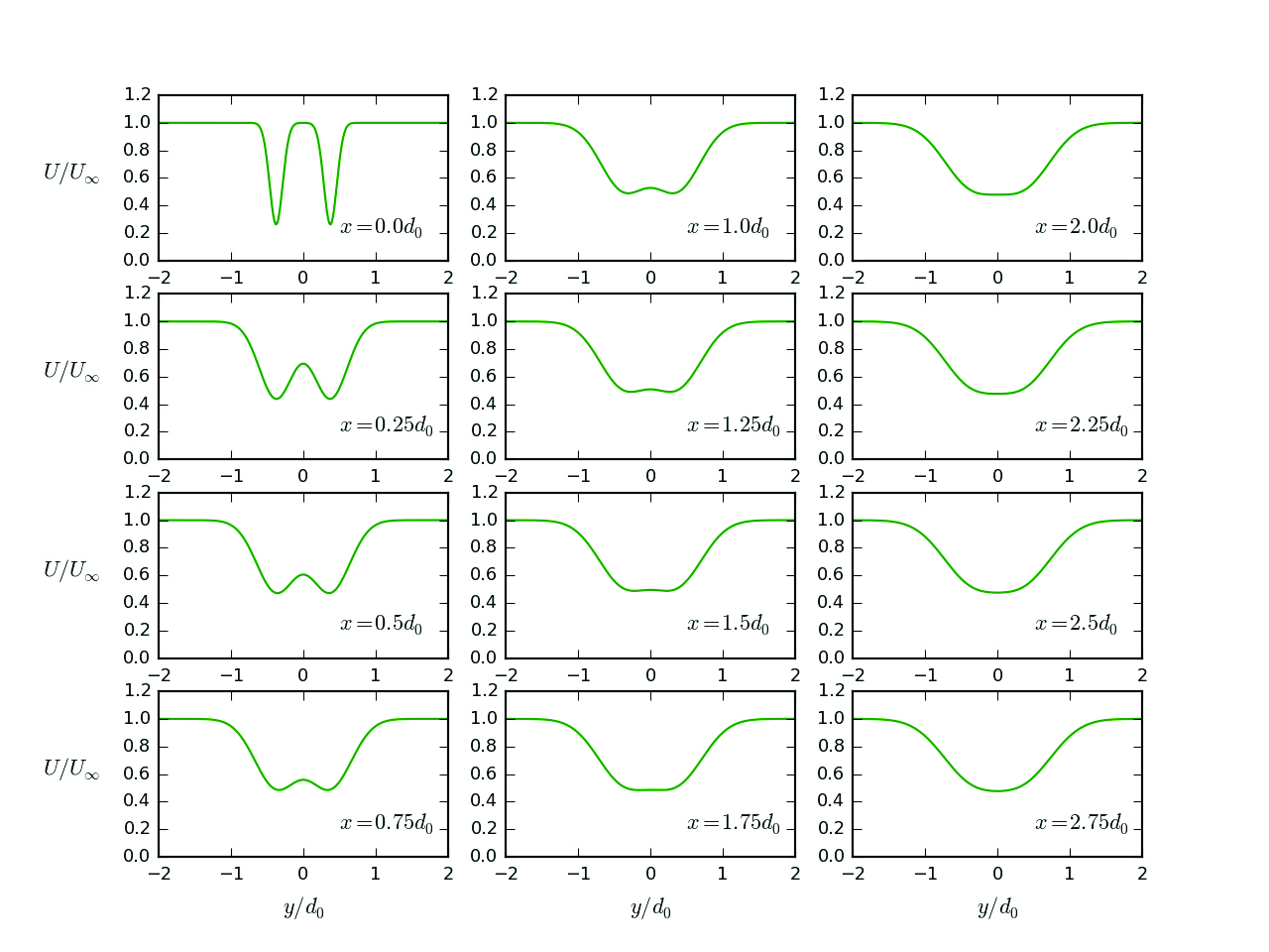
Figure 4: The wind velocity profiles for the hub height horizontal cross-sections through the wake model, for $U_{\infty}=11ms^{-1}$, for various downwind distances $x$. The relevant parameter values are given in Table 1. It is clear that there is a transition from double-Gaussian to single-Gaussian distribution at a downwind distance of about $2.5d_{0}$.

In summary, the real wake velocity solution is

$$U=c_{-}U_{\infty}\biggl{(}1-C_{-}(x)f(r,\sigma(x))\biggr{)}+c_{\infty}U_{\infty},\qquad c_{-}+c_{\infty}=1.$$ (23)

With a further little bit of algebra this can be written as

$$U=U_{\infty}\biggl{(}1-c_{-}C_{-}(x)f(r,\sigma(x))\biggr{)}.$$ (24)

The functions $C_{-}(x)$, $f(r,\sigma(x))$ and $\sigma(x)$ are given by equations (16), (5) and (17) respectively. The function $C_{-}(x)$ is given in terms of the functions $M$ and $N$ defined in equations (14). The real wake velocity solution depends upon several parameters: The wind turbine rotor diameter $d_{0}$, the radial location of the local minimum which has been determined empirically as $r_{0}=0.75d_{0}/2$, $C_{T}$ which is fixed by the wind turbine’s thrust characteristics and varies with inflow wind speed $U_{\infty}$, and the parameters $k^{*}$, $\epsilon$ and $c_{-}$ are obtained from fitting (see next section).

It can be seen from equation (24) that the method is mathematically equivalent to a simple re-scaling of the value of $C_{-}(x)$ by the amount $c_{-}$.

3 Comparison with wake data measurements

The wake model was compared to measured wind turbine wake data obtained in the analysis of Gallacher and More [11], which used nacelle-mounted LiDAR measurements to examine wake length, width and height for a single wind turbine with $d_{0}=116$ m.

Figure 5: Horizontal normalized velocity profile for the wake centreline at hub height for the ($10$ minute averaged) wake data [11], the Jensen model (blue), and the newly proposed model (green). The velocity profiles are shown for $U_{\infty}=7,11$, and $17ms^{-1}$. The rotor diameter $d_{0}=116$ m. Table 1 gives the corresponding best fit parameter values.

Figure 5 shows the wake centreline hub height velocity profile of the new wake model for $U_{\infty}=7,11$, and $17ms^{-1}$, in close agreement with the ($10$ minute averaged) measured wake data. Table 1 gives the corresponding best fit parameter values. The values of $C_{T}$ were looked up for each inflow windspeed based on the wind turbine data. The corresponding Jensen model (see, for example, equation (1) of [3]),

$${\Delta U\over U_{\infty}}=\biggl{(}1-\sqrt{1-C_{T}}\biggr{)}\biggl{(}1+{{2k_{wake}x}\over d_{0}}\biggr{)}^{-2}$$ (25)

with wake decay coefficient $k_{wake}=0.038$ [11], is shown for comparison. (Alternative values are given in, for example, reference [3].) The predicted velocity profile shows a clear local minimum at a distance of about $2$ rotor diameters, in contrast to the Jensen model.

A comparison was made between the nacelle-mounted LiDAR radial velocity measurements of [11] and the corresponding radial velocities given by the wake model. Figure 6 shows the horizontal normalized radial velocity profiles for the wake cross-sections at hub height for the ($10$ minute averaged) wake data, and the newly proposed model, based on the centreline hub height best fit parameter values given in table 1.

Table 1: The model parameters, given to 3 significant figures, for the fitting to the measured centreline hub height wake data. The rotor diameter $d_{0}=116$ m.

Windspeed bin (m/s)	$U_{\infty}(m/s)$	$a$	$C_{T}$	$k^{*}$	$\epsilon$	$c_{-}$
6 - 8	$7$	$0.293$	$0.828$	$6.54$	$0.040$	$0.437$
10 - 12	$11$	$0.256$	$0.761$	$5.40$	$0.090$	$0.400$
16 - 18	$17$	$0.053$	$0.201$	$2.18$	$0.250$	$0.313$

Figure 6: Horizontal normalized nacelle-mounted LiDAR radial velocity profile for the wake cross-sections at hub height for the ($10$ minute averaged) wake data [11], and the newly proposed model, for $U_{\infty}=11ms^{-1}$ and selected downwind distances $x$, based on the centreline hub height best fit parameter values given in table 1. The rotor diameter $d_{0}=116$ m. The magnitude of the LiDAR measured radial velocity tends to zero for large distances from the wake centreline, in contrast to the situation in Figure 4. This effect is particularly evident for small downwind distances and is due to the cosine factor arising as a result of the angular dependence of the LiDAR scan geometry.

4 Discussion

It can be seen from Figures 5 and 6 that the new proposed wake model is in close agreement with the measured data. In Figure 5 the proposed model performs better than the corresponding Jensen model which, when compared to the measured data, exhibits an unphysical drop off in the centreline wake velocity. Figure 6 shows the horizontal hub height radial velocity profiles, and those predicted by the wake model, based on the centreline hub height best fit parameter values. The model performs reasonably well in the near wake region, exhibiting the expected local minima, and showing better agreement with increasing downwind distance. The deviations from perfect fits in the profiles in Figure 5 could in part be attributed to a slightly asymmetric wake profile about the rotor axis, evident in Figure 6, and the presence of other wind turbines.

The proposed wake model is limited by being axially symmetric about the rotor axis. However, the inclusion of vertical wind shear shall be considered in a subsequent publication. The comparison given above are based upon 1D fitting, and only for the wake centreline hub height measurements. Future improvements can be made by simultaneous 2D fitting to wake cross-section hub height data, and possibly full 3D fitting to an entire wake.

5 Conclusions

An analytical wind turbine wake model has been proposed to predict the wind velocity distribution for all distances downwind of a wind turbine, including the near-wake. The model is derived by applying conservation of mass and momentum in the context of actuator disk theory, and assuming a distribution of the double-Gaussian type (5) for the velocity deficit in the wake. The physical solutions are obtained by appropriate mixing of the waked- and freestream velocity deficit solutions through equation (22), reflecting the fact that only a portion of the fluid particles passing through the rotor disk will interact with a blade. As mentioned previously, this is mathematically equivalent to a simple re-scaling of the velocity deficit. The wake model can be used by selecting a wind speed regime, and consulting Table 1 to obtain the corresponding parameter values to provide an appropriate set of values $\{C_{T},k^{*},\epsilon,c_{-}\}$.

The proposed wake model is a development of actuator disk theory, but without the complications of full blade element momentum theory. It has potential for applications to windfarm modeling, with the possibility of incorporating multiple wind turbine wakes. With further development there is the potential for comparison with Large-eddy simulations. The model may also serve to illuminate the physics of the near-wake. Turbulence intensity and dynamic features of the wake important for load modeling have not been considered here. This wake model will be developed further in a subsequent publication, where consideration will be given to inclusion of wind shear, power production and yaw effects.

Appendix

Define

$$J=\int^{r=\infty}_{r=0}\biggl{[}E_{+}+E_{-}-\case{1}{2}C(x)(F_{+}+F_{-}+2G)\biggr{]}rdr$$ (31)

where

$$E_{\pm}=\exp D_{\pm},\qquad F_{\pm}=\exp(2D_{\pm}),\qquad G=\exp(D_{+}+D_{-}),$$ (32)

so that the original integral can be written

$$I=\pi U^{2}_{\infty}C(x)J.$$ (33)

Now consider each term separately. The upper limit of the integration will be taken as $r=R$, which will later be set to $\infty$. Define

$$J_{1}=\int^{r=R}_{r=0}E_{+}rdr$$ (34)

and the new variable

$$r^{\prime}=r+r_{0},\qquad dr^{\prime}=dr.$$ (35)

Then

$$J_{1} =\int^{r^{\prime}=R+r_{0}}_{r^{\prime}=r_{0}}\exp(-\case{1}{2}\sigma^{-2}r^{\prime 2})(r^{\prime}-r_{0})dr^{\prime}$$

$$=\int^{r^{\prime}=R+r_{0}}_{r^{\prime}=r_{0}}\exp(-\case{1}{2}\sigma^{-2}r^{\prime 2})r^{\prime}dr^{\prime}-r_{0}\int^{r^{\prime}=R+r_{0}}_{r^{\prime}=r_{0}}\exp(-\case{1}{2}\sigma^{-2}r^{\prime 2})dr^{\prime}.$$ (36)

These last integrals are of the form

$$\int\exp(x^{2})xdx\qquad\mbox{and}\qquad\int\exp(x^{2})dx$$ (37)

respectively. The former is straightforward to integrate, and the second requires use of the complementary error function [16]

$$\mathrm{erfc}(x)={2\over\sqrt{\pi}}\int^{t=\infty}_{t=x}\exp(-t^{2})dt.$$ (38)

Making the change of variables $r^{\prime}=\sqrt{2}\sigma t$ this becomes

$$\mathrm{erfc}(x)=\sqrt{2\over\pi}\sigma^{-1}\int^{r^{\prime}=\infty}_{r^{\prime}=r_{0}}\exp(-\case{1}{2}\sigma^{-2}r^{\prime 2})dr^{\prime}$$ (39)

where $r_{0}=\sqrt{2}\sigma x$. Similarly, for

$$J_{2}=\int^{r=R}_{r=0}E_{-}rdr$$ (40)

define the new variable

$$r^{\prime\prime}=r-r_{0},\qquad dr^{\prime\prime}=dr.$$ (41)

and so

$$\fl J_{2}=\int^{r^{\prime\prime}=R-r_{0}}_{r^{\prime\prime}=-r_{0}}\exp(-\case{1}{2}\sigma^{-2}r^{\prime\prime 2})r^{\prime\prime}dr^{\prime\prime}+r_{0}\int^{r^{\prime\prime}=R-r_{0}}_{r^{\prime\prime}=-r_{0}}\exp(-\case{1}{2}\sigma^{-2}r^{\prime\prime 2})dr^{\prime\prime}.$$ (42)

Taking $R=\infty$, the sum of the first terms in $J_{1}+J_{2}$ is

$$2\sigma^{2}\exp(-\case{1}{2}\sigma^{-2}r_{0}^{2}).$$ (43)

It follows that the sum of the second terms in the integrals is equal to

$$\sqrt{\pi\over 2}r_{0}\sigma\biggl{[}\mathrm{erfc}\biggl{(}{r_{0}\sigma^{-1}\over\sqrt{2}}\biggr{)}-\mathrm{erfc}\biggl{(}{-r_{0}\sigma^{-1}\over\sqrt{2}}\biggr{)}\biggr{]}.$$ (44)

Further, since

$$\mathrm{erfc}(-x)=2-\mathrm{erfc}(x)$$ (45)

it follows that this sum is equal to

$$\sqrt{2\pi}r_{0}\sigma\biggl{[}\mathrm{erfc}\biggl{(}{r_{0}\sigma^{-1}\over\sqrt{2}}\biggr{)}-1\biggr{]}.$$ (46)

Thus

$$J_{1}+J_{2}=2\sigma^{2}\exp(-\case{1}{2}\sigma^{-2}r_{0}^{2})+\sqrt{2\pi}r_{0}\sigma\biggl{[}\mathrm{erfc}\biggl{(}{r_{0}\sigma^{-1}\over\sqrt{2}}\biggr{)}-1\biggr{]}.$$ (47)

Similarly, defining

$$J_{3}=\int^{r=\infty}_{r=0}F_{+}rdr,\qquad J_{4}=\int^{r=\infty}_{r=0}F_{-}rdr$$ (48)

it can be shown that

$$J_{3}+J_{4}=\sigma^{2}\exp(-\sigma^{-2}r_{0}^{2})+\sqrt{\pi}r_{0}\sigma\biggl{[}\mathrm{erfc}(r_{0}\sigma^{-1})-1\biggr{]}.$$ (49)

Finally, defining

$$J_{5}=\int^{r=\infty}_{r=0}Grdr$$ (50)

it follows that

$$J_{5}=\int^{r=\infty}_{r=0}\exp[-\sigma^{-2}(r^{2}+r_{0}^{2})]rdr=\case{1}{2}\sigma^{2}\exp[-\sigma^{-2}r_{0}^{2}].$$ (51)

References

References

- [1] Jensen NO 1983 Risø National Laboratory Report M-2411
- [2] Frandsen S, Barthelmie R, Pryor S, Rathmann O, Larsen S, Højstrup J, Thøgersen M. (2006), Analytical modelling of wind speed deficit in large offshore wind farms. Wind Energ., 9: 39 53.
- [3] Bastankhah M and Porté-Agel F 2014 Renewable Energy 70 116
- [4] Ainslie JF 1988 J. Wind Eng. Ind. Aerodyn. 27 213-224
- [5] Larsen GC 1988 Risø National Laboratory Report M-2760
- [6] Larsen GC, Højstrup J and Madsen HA 1996 Wind Fields in Wakes , Proceedings EWEC ’96, 764
- [7] Crespo A, Hernández J, Fraga E and Andreu C 1988 J. Wind Eng. Ind. Aerodyn. 27 77-88
- [8] Magnusson M 1999 J. Wind Eng. Ind. Aerodyn. 80 147-167
- [9] Okulov VL, Naumov IV, Mikkelsen RF, Sørensen JN 2015 Journal of Physics: Conference Series 625 012011
- [10] Mirocha JD, Rajewski DA, Marjanovic N, Lundquist JK, Kosović B, Draxl C, Churchfield MJ 2015 J. Renewable Sustainable Energy 7 043143
- [11] Gallacher D, More G 2014 EWEA-2014-Poster Lidar Measurements and Visualisation of Turbulence and Wake Decay Length (SgurrEnergy)
- [12] Vermeer LJ, Sørensen JN, Crespo A 2003 Progress in Aerospace Sciences 39 467-510
- [13] Aitken ML, Banta RM, Pichugina YL, Lundquist JK 2014 J. Atmos. Oceanic Technol. 31 765 787
- [14] Burton T, Jenkins N, Sharpe D, Bossanyi E 2011 Wind Energy Handbook, 2nd Edition, (John Wiley & Sons)
- [15] Tennekes H and Lumley JL 1972 A First course in turbulence, (The MIT Press)
- [16] Stephenson G and Radmore P M Advanced Mathematical Methods for Engineering and Science Students, (Cambridge: Cambridge University Press) 1990