Task-based parallelization of an implicit kinetic scheme

Abstract.

In this paper we present and implement the Palindromic Discontinuous Galerkin (PDG) method in dimensions higher than one. The method has already been exposed and tested in [4] in the one-dimensional context. The PDG method is a general implicit high order method for approximating systems of conservation laws. It relies on a kinetic interpretation of the conservation laws containing stiff relaxation terms. The kinetic system is approximated with an asymptotic-preserving high order DG method. We describe the parallel implementation of the method, based on the StarPU runtime library. Then we apply it on preliminary test cases.

1. Introduction

In this work we consider the time discretization of compressible fluid models that appear in gas dynamics, biology, astrophysics or plasma physics for tokamaks. These models can be unified in the following form

(1.1) $$\partial_{t}\mathbf{w}+\sum_{k=1}^{D}\partial_{k}\mathbf{q}^{k}(\mathbf{w})=\mathbf{{s}},$$

where $\mathbf{w}:\mathbb{R}^{D}\times[0,T_{\max}]\longrightarrow\mathbb{R}^{m}$ is the vector of conservative variables, $\mathbf{q}^{k}(\mathbf{w}):\mathbb{R}^{m}\longrightarrow\mathbb{R}^{m}$ is the flux and $\mathbf{{s}}:\mathbb{R}^{D}\times\mathbb{R\times R}^{m}\longrightarrow\mathbb{R}^{m}$ is a source term. $D$ represents the physical space dimension and $m$ the number of unknowns.

In many physical applications such as MHD flows, low Mach Euler equations, Shallow-Water with sedimentation, the model presents several time scales associated to the propagation of different waves. When the time scale of fast phenomena, which constrains the explicit CFL condition, is very small compared to the time scale of the most relevant phenomena, it becomes necessary to switch to implicit schemes. However classical implicit schemes are very costly in 2D or 3D because they require the resolution of linear or non-linear systems at each time step. In addition, the matrices associated with the hyperbolic systems are generally ill-conditioned.

In this paper, we propose to follow another approach for avoiding the resolution of complicated linear systems. Instead of solving the full fluid model (1.1) directly, we replace it by a simpler kinetic interpretation made of a set of transport equations coupled through a stiff relaxation term [1, 3, 7]. See also [4] and included references. The kinetic system is then solved by a splitting method where the transport and relaxation stages are treated separately. The method is then well adapted to parallel optimizations. The method is already presented in [4] in the one-dimensional case. Here we present its implementation in higher dimensions. We particularly focus our presentation of the massive parallelization of the method with the StarPU runtime system [2].

The outlines are as follows.

First we recall that it is possible to provide a general kinetic interpretation of any system of conservation laws. The interest of this representation is that the complicated non-linear system is replaced by a (larger) set of scalar linear transport equations that are much easier to solve. The transport equations are coupled through a non-linear source term that is fully local in space.

Then, we detail the approximation which allows to solve the transport equation in an efficient way. We adopt a Discontinuous Galerkin (DG) method based on an upwind numerical flux and Gauss-Lobatto quadrature points. Thanks to the upwind flux, the matrix of the discretized transport operator has a block-triangular structure.

The main part of this work is devoted to the task parallelization based on the StarPU library for treating the transport and relaxation steps efficiently. We use the MPI version of StarPU, which allows to address clusters of multicore processors. We also describe the domain decomposition and the macrocell approach that we have used to achieve better performance.

Finally, we give some numerical results for measuring the efficiency of the parallelism and the ability of the method to compute realistic problems.

2. Kinetic model

We consider the following kinetic equation

(2.1) $$\partial_{t}\mathbf{{f}}+\sum_{k=1}^{D}\mathbf{V}^{k}\partial_{k}\mathbf{{f}}=\frac{1}{\tau}(\mathbf{{f}}^{eq}(\mathbf{{f}})-\mathbf{{f}})+\mathbf{{g}}.$$

The unknown is a vectorial distribution function $\mathbf{{f}}(\mathbf{x},t)\in\mathbb{R}^{n_{v}}$ depending on the space variable $\mathbf{x}=(x^{1}\ldots x^{D})\in\mathbb{R}^{D}$ and time $t\in\mathbb{R}$. $\mathbf{{g}}(\mathbf{x},t,\mathbf{f})$ is a vectorial source term, possibly depending on space, time and $\mathbf{{f}}$. The partial derivatives are noted

$$\partial_{t}=\frac{\partial}{\partial t},\quad\partial_{k}=\frac{\partial}{\partial x^{k}}.$$

The relaxation time $\tau$ is a small positive constant. The constant matrices $\mathbf{V}^{k}$, $1\leq k\leq D$ are diagonal

$$\mathbf{V}^{k}=\left(\begin{array}[]{cccc}v_{1}^{k}\\ &v_{2}^{k}\\ &&\ddots\\ &&&v_{n_{v}}^{k}\end{array}\right)$$

In other words, (2.1) is a set of $n_{v}$ transport equations at constant velocities $\mathbf{v}_{i}=(v_{i}^{1},\ldots,v_{i}^{D})$, coupled through a stiff BGK relaxation, and with an optional additional source term. We denote by $\mathbf{V\cdot\boldsymbol{\partial}}=\sum_{k=1}^{D}\mathbf{V}^{k}\partial_{k}$ the transport operator, and by $\mathbf{N\mathbf{{f}}}=(\mathbf{{f}}^{eq}(\mathbf{{f}})-\mathbf{{f}})/\tau$ the BGK relaxation term (also called the “collision” term).

Generally, this kinetic model represents an underlying hyperbolic system of conservation laws. The macroscopic conservative variables $\mathbf{w}(\mathbf{x},t)\in\mathbb{R}^{m}$ are obtained through a linear transformation

(2.2) $$\mathbf{w}=\mathbf{P}\mathbf{{f}},$$

where $\mathbf{P}$ is a $m\times n_{v}$ matrix. Generally the number of conservative variables is smaller than the number of kinetic data: $m<n_{v}$. The equilibrium (or “Maxwellian”) distribution $\mathbf{{f}}^{eq}(\mathbf{{f}})$ is such that

$$\mathbf{Pf}=\mathbf{P}\mathbf{{f}}^{eq}(\mathbf{{f}}),$$

and

(2.3) $$\mathbf{w}=\mathbf{P}\mathbf{{f}}_{1}=\mathbf{P}\mathbf{f_{2}}\Rightarrow\mathbf{{f}}^{eq}(\mathbf{{f}}_{1})=\mathbf{{f}}^{eq}(\mathbf{f_{2}}),$$

which states that the equilibrium actually depends only on the macroscopic data $\mathbf{w}$. We could have used the notation $\mathbf{{f}}^{eq}=\mathbf{{f}}^{eq}(\mathbf{w})=\mathbf{{f}}^{eq}(\mathbf{P}\mathbf{{f}})$, but we have decided to respect a well-established tradition.

When $\tau\to 0$, the kinetic equations provide an approximation of the system of conservation laws

(2.4) $$\partial_{t}\mathbf{w}+\sum_{k=1}^{D}\partial_{k}\mathbf{q}^{k}(\mathbf{w})=\mathbf{{s}},$$

where the flux is given by

$$\mathbf{q}^{k}(\mathbf{w})=\mathbf{P}\mathbf{V}^{k}\mathbf{{f}}^{eq}(\mathbf{{f}}).$$

The flux is indeed a function of $\mathbf{w}$ only because of (2.3).

Similarly the source term is given by

(2.5) $$\mathbf{{s}}(\mathbf{x},t,\mathbf{w})=\mathbf{P}\mathbf{{g}}(\mathbf{x},t,\mathbf{{f}}^{eq})$$

System (2.1) has to be supplemented with conditions at the boundary $\partial\Omega$ of the computational domain $\Omega$. We denote by $\mathbf{n}=(n_{1}\ldots n_{D})$ the outward normal vector on $\partial\Omega.$ For simplicity, we shall only consider very simple imposed and time-independent boundary conditions $\mathbf{{f}}^{b}$. We note

$$\mathbf{V}\cdot\mathbf{n}=\sum_{k=1}^{D}\mathbf{V}^{k}n_{k},\quad\mathbf{V}\cdot\mathbf{n}^{+}=\max(\mathbf{V}\cdot\mathbf{n},0),\quad\mathbf{V}\cdot\mathbf{n}^{-}=\min(\mathbf{V}\cdot\mathbf{n},0).$$

A natural boundary condition, which is compatible with the transport operator $\mathbf{V\cdot\boldsymbol{\partial}}$, is

(2.6) $$\mathbf{V}\cdot\mathbf{n}^{-}\mathbf{{f}}(\mathbf{x},t)=\mathbf{V}\cdot\mathbf{n}^{-}\mathbf{{f}}^{b}(\mathbf{x}),\quad\mathbf{x}\in\partial\Omega.$$

It states that for a given velocity $\mathbf{v}_{i}$, the corresponding boundary data $f_{i}^{b}$ is used only at the inflow part of the boundary.

Let us point out that the programming optimization that we propose in this paper rely in an essential way on the nature of the boundary condition (2.6). For other boundary conditions, such as periodic or wall conditions, additional investigations are still needed.

3. Numerical method

3.1. Discontinuous Galerkin approximation

For solving (2.1) we shall treat the transport operator $\mathbf{V}\cdot\boldsymbol{\partial}$ and the collision operator $\mathbf{N}$ efficiently, thanks to a splitting approach. This allows to achieve a better parallelism. Let us start with the description of the transport solver.

For a simple exposition, we only consider one single scalar transport equation for $f(\mathbf{x},t)\in\mathbb{R}$ at constant velocity $\mathbf{v}$

(3.1) $$\partial_{t}f+\mathbf{v}\cdot\nabla f=0.$$

The general vectorial case is easily deduced.

We consider a mesh $\mathcal{M}$ of $\Omega$ made of open sets, called “cells”, $\mathcal{M}=\left\{L_{i},\,i=1\ldots N_{c}\right\}$. In the most general setting, the cells satisfy

1. $L_{i}\cap L_{j}=\emptyset$, if $i\neq j$;

2. $\overline{\cup_{i}L_{i}}=\overline{\Omega}.$

In each cell $L\in\mathcal{M}$ we consider a basis of functions $(\varphi_{L,i}(\mathbf{x}))_{i=0\ldots N_{d}-1}$ constructed from polynomials of order $d$. We denote by $h$ the maximal diameter of the cells. With an abuse of notation we still denote by $f$ the approximation of $f$, defined by

$$f(\mathbf{x},t)=\sum_{j=0}^{N_{d}-1}f_{L,j}(t)\varphi_{L,j}(\mathbf{x}),\quad\mathbf{x}\in L.$$

The DG formulation then reads: find the $f_{L,j}$’s such that for all cell $L$ and all test function $\varphi_{L,i}$

(3.2) $$\int_{L}\partial_{t}f\varphi_{L,i}-\int_{L}f\mathbf{v}\cdot\nabla\varphi_{L,i}+\int_{\partial L}(\mathbf{v}\cdot\mathbf{n}^{+}f_{L}+\mathbf{v}\cdot\mathbf{n}^{-}f_{R})\varphi_{L,i}=0.$$

In this formula (see Figure 4.1):

• $R$ denotes the neighboring cell to $L$ along its boundary $\partial L\cap\partial R$, or the exterior of $\Omega$ on $\partial L\cap\partial\Omega$.

• $\mathbf{n}=\mathbf{n}_{LR}$ is the unit normal vector on $\partial L$ oriented from $L$ to $R$.

• $f_{R}$ denotes the value of $f$ in the neighboring cell $R$ on $\partial L\cap\partial R$.

• If $L$ is a boundary cell, one may have to use the boundary values instead: $f_{R}=f^{b}$ on $\partial L\cap\partial\Omega$.

• $\mathbf{v}\cdot\mathbf{n}^{+}f_{L}+\mathbf{v}\cdot\mathbf{n}^{-}f_{R}$ is the standard upwind numerical flux encountered in many finite volume or DG methods.

Figure 3.1. Convention for the $L$ and $R$ cells orientation.

In our application, we consider hexahedral cells. We have a reference cell

$$\hat{L}=]-1,1[^{D}$$

and a smooth transformation $\mathbf{x}=\boldsymbol{\tau}_{L}(\hat{\mathbf{x}})$, $\hat{\mathbf{x}}\in\hat{L}$, that maps $\hat{L}$ on $L$

$$\boldsymbol{\tau}_{L}(\hat{L})=L.$$

We assume that $\boldsymbol{\tau}_{L}$ is invertible and we denote by $\boldsymbol{\tau}_{L}^{\prime}$ its (invertible) Jacobian matrix. We also assume that $\boldsymbol{\tau}_{L}$ is a direct transformation

$$\det\boldsymbol{\tau}_{L}^{\prime}>0.$$

In our implementation $\boldsymbol{\tau}_{L}$ is a quadratic map based on hexahedral curved “H20” finite elements with 20 nodes. The mesh of H20 finite elements is generated by gmsh [6].

On the reference cell, we consider the Gauss-Lobatto points $(\hat{\mathbf{x}}_{i})_{i=0\ldots N_{d}-1}$, $N_{d}=(d+1)^{D}$ and associated weights $(\omega_{i})_{i=0\ldots N_{d}-1}$. They are obtained by tensor products of the $(d+1)$ one-dimensional Gauss-Lobatto (GL) points on $]-1,1[$. The reference GL points and weights are then mapped to the physical GL points of cell $L$ by

(3.3) $$\mathbf{x}_{L,i}=\boldsymbol{\tau}_{L}(\hat{\mathbf{x}}_{i}),\quad\omega_{L,i}=\omega_{i}\det\boldsymbol{\tau}_{L}^{\prime}(\hat{\mathbf{x}}_{i})>0.$$

In addition, the six faces of the reference hexahedral cell are denoted by $F_{\epsilon}$, $\epsilon=1\ldots 6$ and the corresponding outward normal vectors are denoted by $\hat{\mathbf{n}}_{\epsilon}$. A big advantage of choosing the GL points is that the volume and the faces share the same quadrature points. A special attention is necessary for defining the face quadrature weights. If a GL point $\hat{\mathbf{x}}_{i}\in F_{\epsilon}$, we denote by $\mu_{i}^{\epsilon}$ the corresponding quadrature weight on face $F_{\epsilon}$. We also use the convention that $\mu_{i}^{\epsilon}=0$ if $\hat{\mathbf{x}}_{i}$ does not belong to face $F_{\epsilon}$. A given GL point $\hat{\mathbf{x}}_{i}$ can belong to several faces when it is on an edge or in a corner of $\hat{L}$. Because of symmetry, we observe that if $\mu_{i}^{\epsilon}\neq 0$, then the weight $\mu_{i}^{\epsilon}$ does not depend on $\epsilon$.

We then consider basis functions $\hat{\varphi_{i}}$ on the reference cell: they are the Lagrange polynomials associated to the Gauss-Lobatto point and thus satisfy the interpolation property

$$\hat{\varphi}_{i}(\hat{\mathbf{x}}_{j})=\delta_{ij}.$$

The basis functions on cell $L$ are then defined according to the formula

$$\varphi_{L,i}(\mathbf{x})=\hat{\varphi}_{i}(\boldsymbol{\tau}_{L}^{-1}(\mathbf{x})).$$

In this way, they also satisfy the interpolation property

(3.4) $$\varphi_{L,i}(\mathbf{x}_{L,j})=\delta_{ij}.$$

In this paper, we only consider conformal meshes: the GL points on cell $L$ are supposed to match the GL points of cell $R$ on their common face. Dealing with non-matching cells is the object of a forthcoming work.

Let $L$ and $R$ be two neighboring cells. Let $\mathbf{x}_{L,j}$ be a GL point in cell $L$ that is also on the common face between $L$ and $R$. In the case of conformal meshes, it is possible to define the index $j^{\prime}$ such that

$$\mathbf{x}_{L,j}=\mathbf{x}_{R,j^{\prime}}.$$

Applying a numerical integration to (3.2), using (3.3) and the interpolation property (3.4), we finally obtain

(3.5) $$\partial_{t}f_{L,i}\omega_{L,i}-\sum_{j=0}^{N_{d}-1}\mathbf{v}\cdot\nabla\varphi_{L,i}(\mathbf{x}_{L,j})f_{L,j}\omega_{L,j}+\\ \sum_{\epsilon=1}^{6}\mu_{i}^{\epsilon}\left(\mathbf{v}\cdot\mathbf{n}_{\epsilon}(\mathbf{x}_{L,i})^{+}f_{L,i}+\mathbf{v}\cdot\mathbf{n}_{\epsilon}(\mathbf{x}_{L,i})^{-}f_{R,i^{\prime}}\right)=0.$$

We have to detail how the gradients and normal vectors are computed in the above formula. Let $\mathbf{A}$ be a square matrix. We recall that the cofactor matrix of $\mathbf{A}$ is defined by

(3.6) $$\text{co}(\mathbf{A})=\det(\mathbf{A})\left(\mathbf{A}^{-1}\right)^{T}.$$

The gradient of the basis function is computed from the gradients on the reference cell using (3.6)

$$\nabla\varphi_{L,i}(\mathbf{x}_{L,j})=\frac{1}{\det\boldsymbol{\tau}_{L}^{\prime}(\hat{\mathbf{x}}_{i})}\text{co}(\boldsymbol{\tau}_{L}^{\prime}(\hat{\mathbf{x}}_{j}))\hat{\nabla}\hat{\varphi}_{i}(\hat{\mathbf{x}}_{j}).$$

In the same way, the scaled normal vectors $\mathbf{n}_{\epsilon}$ on the faces are computed by the formula

$$\mathbf{n}_{\epsilon}(\mathbf{x}_{L,i})=\text{co}(\boldsymbol{\tau}_{L}^{\prime}(\hat{\mathbf{x}}_{i}))\hat{\mathbf{n}}_{\epsilon}.$$

We introduce the following notation for the cofactor matrix

$$\mathbf{c}_{L,i}=\text{co}(\boldsymbol{\tau}_{L}^{\prime}(\hat{\mathbf{x}}_{i})).$$

The DG scheme then reads

(3.7) $$\partial_{t}f_{L,i}-\frac{1}{\omega_{L,i}}\sum_{j=0}^{N_{d}-1}\mathbf{v}\cdot\mathbf{c}_{L,j}\hat{\nabla}\hat{\varphi}_{i}(\hat{\mathbf{x}}_{j})f_{L,j}\omega_{j}+\\ \frac{1}{\omega_{L,i}}\sum_{\epsilon=1}^{6}\mu_{i}^{\epsilon}\left(\mathbf{v}\cdot\mathbf{c}_{L,i}\hat{\mathbf{n}}_{\epsilon}{}^{+}f_{L,i}+\mathbf{v}\cdot\mathbf{c}_{L,i}\hat{\mathbf{n}}_{\epsilon}{}^{-}f_{R,i^{\prime}}\right)=0.$$

On boundary GL points, the value of $f_{R,i^{\prime}}$ is given by the boundary condition

$$f_{R,i^{\prime}}=f^{b}(\mathbf{x}_{L,i}),\quad\mathbf{x}_{L,i}=\mathbf{x}_{R,i^{\prime}}.$$

For practical reasons, it is interesting to also consider $f_{R,i^{\prime}}$ as an artificial unknown in the fictitious cell. The fictitious unknown is then a solution of the differential equation

(3.8) $$\partial_{t}f_{R,i^{\prime}}=0.$$

In the end, if we put all the unknowns in a large vector $\mathbf{F}(t)$, (3.7), (3.8) read as a large system of coupled differential equations

(3.9) $$\partial_{t}\mathbf{F}=\mathbf{L}_{h}\mathbf{F}.$$

In the following, we call $\mathbf{L}_{h}$ the transport matrix. The transport matrix satisfies the following properties:

• $\mathbf{L}_{h}\mathbf{F}=0$ if the components of $\mathbf{F}$ are all the same.

• Let $\mathbf{F}$ be such that the components corresponding to the boundary term vanish. Then $\mathbf{F}^{T}\mathbf{L}_{h}\mathbf{F}\leq 0$. This dissipation property is a consequence of the choice of an upwind numerical flux [9].

• In many cases, and with a good numbering of the unknowns in $\mathbf{F}$, $\mathbf{L}_{h}$ has a triangular structure. This aspect is discussed in Subsection 4.1.

As stated above, we actually have to apply a transport solver for each constant velocity $\mathbf{v}_{i}$.

Let $L$ be a cell of the mesh $\mathcal{M}$ and $\mathbf{x}_{i}$ a GL point in $L$. As in the scalar case, we denote by $\mathbf{{f}}_{L,i}$ the approximation of $\mathbf{{f}}$ in $L$ at GL point $i$. In the sequel, with an abuse of notation and according to the context, we may continue to note $\mathbf{F}(t)$ the big vector made of all the vectorial values $\mathbf{{f}}_{L,j}$ at all the GL points $j$ in all the (real or fictitious) cells $L$.

We may also continue to denote by $\mathbf{L}_{h}$ the matrix made of the assembly of all the transport operators for all velocities $\mathbf{v}_{i}$. With a good numbering of the unknowns it is possible in many cases to suppose that $\mathbf{L}_{h}$ is block-triangular. More precisely, because in the transport step the equations are uncoupled, we see that $\mathbf{L}_{h}$ can be made block-diagonal, each diagonal block being itself block-triangular. See Section 4.1.

3.2. Palindromic time integration

We can also define an approximation $\mathbf{N}_{h}$ of the collision operator $\mathbf{N}$. We define by $\mathbf{F}^{eq}(\mathbf{F})$ the big vector made of all the $\mathbf{{f}}^{eq}(\mathbf{{f}}_{L,i})$, $L\in\mathcal{M},$ $i=0\ldots N_{d}-1.$

We set

(3.10) $$\mathbf{N}_{h}\mathbf{F}=\frac{1}{\tau}(\mathbf{F}^{eq}(\mathbf{F})-\mathbf{F}).$$

Similarly we note $\mathbf{G}_{h}$ the discrete approximation of the kinetic source term $\mathbf{{g}}$.

The DG approximation of (2.1) finally reads

$$\partial_{t}\mathbf{F}=\mathbf{L}_{h}\mathbf{F}+\mathbf{N}_{h}\mathbf{F}+\mathbf{G}_{h}\mathbf{F}.$$

We use the following Crank-Nicolson second order time integrator for the transport equation:

(3.11) $$\exp(\Delta t\mathbf{L}_{h})\simeq T_{2}(\Delta t):=(\mathbf{I}+\frac{\Delta t}{2}\mathbf{L}_{h})(\mathbf{I}-\frac{\Delta t}{2}\mathbf{L}_{h})^{-1}.$$

Similarly, for the collision integrator, we use

$$\exp(\Delta t\mathbf{N}_{h})\simeq C_{2}(\Delta t):=(\mathbf{I}+\frac{\Delta t}{2}\mathbf{N}_{h})(\mathbf{I}-\frac{\Delta t}{2}\mathbf{N}_{h})^{-1}.$$

Because during the collision step, the conservative variables $\mathbf{w}=\mathbf{P}\mathbf{{f}}$ do not change, the collision integrator is only apparently implicit. We have the explicit formula:

(3.12) $$C_{2}(\Delta t)\mathbf{F}=\frac{(2\tau-\Delta t)\mathbf{F}}{2\tau+\Delta t}+\frac{2\Delta t\mathbf{F}^{eq}(\mathbf{F})}{2\tau+\Delta t}.$$

The source operator is also approximated by a Crank-Nicolson integrator

$$\exp(\Delta t\mathbf{G}_{h})\simeq S_{2}(\Delta t):=(\mathbf{I}+\frac{\Delta t}{2}\mathbf{G}_{h})(\mathbf{I}-\frac{\Delta t}{2}\mathbf{G}_{h})^{-1},$$

requiring to solve a nonlinear local equation whenever $\mathbf{{g}}$ depends on $\mathbf{{f}}$.

If $\tau>0$, we observe that the operators $T_{2}$ and $C_{2}$ are time-symmetric: if we set $O_{2}=T_{2}$ , $O_{2}=C_{2}$, or $O_{2}=S_{2}$, then $O_{2}$ satisfies

(3.13) $$O_{2}(-\Delta t)=O_{2}(\Delta t)^{-1},\quad O_{2}(0)=Id.$$

This property implies that $O_{2}$ is necessarily a second order approximation of the exact integrator [10, 8]. When $\tau=0,$ we also remark that

$$C_{2}(\Delta t)\mathbf{F}=2\mathbf{F}^{eq}(\mathbf{F})-\mathbf{F}\neq\mathbf{F}$$

and then $C_{2}$ does not satisfy (3.13) anymore.

For $\tau>0$, the Strang formula permits us to construct a five steps second order time-symmetric approximation

$$M_{2}^{s}(\Delta t)=T_{2}(\frac{\Delta t}{2})S_{2}(\frac{\Delta t}{2})C_{2}(\Delta t)S_{2}(\frac{\Delta t}{2})T_{2}(\frac{\Delta t}{2})=\exp\left(\Delta t\left(\mathbf{L}_{h}+\mathbf{N}_{h}+\mathbf{S}_{h}\right)\right)+O(\Delta t^{3}),$$

and a three step one

$$M_{2}(\Delta t)=T_{2}(\frac{\Delta t}{2})C_{2}(\Delta t)T_{2}(\frac{\Delta t}{2})=\exp\left(\Delta t\left(\mathbf{L}_{h}+\mathbf{N}_{h}\right)\right)+O(\Delta t^{3}),$$

in the source-less case.

However this formula is no more a second order approximation of (2.1) when $\tau\to 0$. Indeed, when $\tau=0$

$$M_{2}(0)\mathbf{F}=2\mathbf{F}^{eq}(\mathbf{F})-\mathbf{F}.$$

As explained in [4] it is better to consider the following method, which remains second order accurate even for infinitely fast relaxation:

$$M_{2}^{kin}(\Delta t)=T_{2}(\frac{\Delta t}{4})C_{2}(\frac{\Delta t}{2})T_{2}(\frac{\Delta t}{2})C_{2}(\frac{\Delta t}{2})T_{2}(\frac{\Delta t}{4}).$$

By palindromic compositions of the second order method $M_{2}^{kin}$ it is then very easy to achieve any even order of accuracy (see [4]). However, in this paper, we concentrate on the parallel optimization of the method and we shall only present numerical results at second order for the limit system 2.4. To that end it is sufficient to use the method $M_{2}$, as $PM_{2}(0)$ properly converges towards identity on the macroscopic variable space when $\tau\rightarrow 0$.

4. Optimization of the kinetic solver

In this section, we describe the optimizations that can be applied in the implementation of the previous numerical method.

4.1. Triangular structure of the transport matrix

Because of the upwind structure of the numerical flux, it appears that the transport matrix is often block-triangular. This is very interesting because this allows to apply implicit schemes to (3.9) without the costly inversion of linear systems [11]. We can provide the formal structure of $\mathbf{L}_{h}$ through the construction of a directed graph $\mathcal{G}$ with a set of vertices $\mathcal{V}$ and a set of edges $\mathcal{E}\subset\mathcal{V}\times\mathcal{V}$. The vertices of the graph are associated to the (real or fictitious) cells of $\mathcal{M}$. Consider now two cells $L$ and $R$ with a common face $F_{LR}$. We denote by $\mathbf{n}_{LR}$ the normal vector on $F_{LR}$ oriented from $L$ to $R$. If there is at least one GL point $\mathbf{x}$ on $F_{LR}$ such that

$$\mathbf{n}_{LR}(\mathbf{x})\cdot\mathbf{v}>0,$$

then the edge from $L$ to $R$ belongs to the graph:

$$(L,R)\in\mathcal{E},$$

see Figure 4.1.

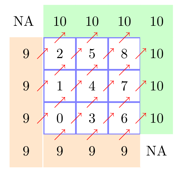
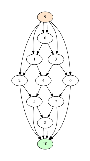
Figure 4.1. Construction of the dependency graph. Left: example of mesh (it is structured here but it is not necessary) with 9 interior cells. The velocity field $v$ is indicated by red arrows. We add two fictitious cells: one for the upwind boundary condition (cell $9$) and one for the outflow part of $\partial\Omega$ (cell $10$). Right: the corresponding dependency graph $\mathcal{G}.$ By examining the dependency graph, we observe that the values of $\mathbf{F}^{n+1}$ in cell $0$ have to be computed first, using the boundary conditions. Then cells $1$ and $3$ can be computed in parallel, then cells $2,$ $4,$ and $6$ can be computed in parallel, then etc.

In (3.7) we can distinguish between several kinds of terms. We write

$$\partial_{t}f_{L}+\Gamma_{L\leftarrow L}f_{L}+\sum_{(R,L)\in\mathcal{E}}\Gamma_{L\leftarrow R}f_{R},$$

with

$$\Gamma_{L\leftarrow L}f_{L}=-\frac{1}{\omega_{L,i}}\sum_{j=0}^{N_{d}-1}\mathbf{v}\cdot\mathbf{c}_{L,j}\hat{\nabla}\hat{\varphi}_{i}(\hat{\mathbf{x}}_{j})f_{L,j}\omega_{j}+\\ \frac{1}{\omega_{L,i}}\sum_{\epsilon=1}^{6}\mu_{i}^{\epsilon}\mathbf{v}\cdot\mathbf{c}_{L,i}\hat{\mathbf{n}}_{\epsilon}{}^{+}f_{L,i},$$

and, if $(R,L)\in\mathcal{E}$,

$$\Gamma_{L\leftarrow R}f_{R}=\frac{1}{\omega_{L,i}}\mu_{i}^{\epsilon}\mathbf{v}\cdot\mathbf{c}_{L,i}\hat{\mathbf{n}}_{\epsilon}{}^{-}f_{R,i^{\prime}}.$$

We can use the following convention

(4.1) $$(R,L)\notin\mathcal{E}\Rightarrow\Gamma_{L\leftarrow R}=0.$$

$\Gamma_{L\leftarrow L}$ contains the terms that couple the values of $f$ inside the cell $L$. They correspond to diagonal blocks of size $(d+1)^{D}\times(d+1)^{D}$ in the transport matrix $\mathbf{L}_{h}$. $\Gamma_{L\leftarrow R}$ contains the terms that couple the values inside cell $L$ with the values in the neighboring upwind cell $R$. If $R$ is a downwind cell relatively to $L$ then $\mu_{i}^{\epsilon}\mathbf{v}\cdot C_{L,i}\hat{\mathbf{n}}_{\epsilon}{}^{-}=0$ and $\Gamma_{L\leftarrow R}=0$ is indeed compatible with the above convention (4.1).

Once the graph $\mathcal{G}$ is constructed, we can analyze it with standard tools. If it contains no cycle, then it is called a Directed Acyclic Graph (DAG). Any DAG admits a topological ordering of its nodes. A topological ordering is a numbering of the cells $i\mapsto L_{i}$ such that if there is a path from $L_{i}$ to $L_{j}$ in $\mathcal{G}$ then $j>i$. In practice, it is useful to remove the fictitious cells from the topological ordering. In our implementation they are put at the end of the list.

Once the new ordering of the graph vertices is constructed, we can construct a numbering of the components of $\mathbf{F}$ by first numbering the unknowns in $L_{0}$ then the unknowns in $L_{1}$, etc. More precisely, we set

$$F_{kN_{d}+i}=f_{L_{k},i}.$$

Then, with this ordering, the matrix $\mathbf{L}_{h}$ is lower block-triangular with diagonal blocks of size $(d+1)^{D}\times(d+1)^{D}$. It means that we can apply implicit schemes to (3.9) without inverting large linear systems.

As stated above, we actually have to apply a transport solver for each constant velocity $\mathbf{v}_{i}$. In the sequel, with another abuse of notation and according to the context, we continue to note $\mathbf{F}$ the big vector made of all the vectorial values $\mathbf{{f}}_{L,j}$ at all the GL points $j$ in all the (real or fictitious) cells $L$.

We may also continue to denote by $\mathbf{L}_{h}$ the matrix made of the assembly of all the transport operators for all velocities $\mathbf{v}_{i}$. With a good numbering of the unknown it is still possible to suppose that $\mathbf{L}_{h}$ is block-triangular. More precisely, as in the transport step the equations are uncoupled, we see that $\mathbf{L}_{h}$ can be made a block-diagonal matrix, each diagonal block being itself block-triangular.

4.2. Parallelization of the implicit solver

In this section, we explain how it is possible to parallelize the transport solver. Here again we consider the single transport equation (3.1) and the associated differential equation (3.9). We apply a second order Crank-Nicolson implicit scheme. We have explained in Section 3.2 how to increase the order of the scheme. We compute an approximation $\mathbf{F}^{n}$ of $\mathbf{F}(n\Delta t$). The implicit scheme reads

(4.2) $$(\mathbf{I}-\Delta t\mathbf{L}_{h})\mathbf{F}^{n+1}=(\mathbf{I}+\Delta t\mathbf{L}_{h})\mathbf{F}^{n}.$$

As explained above, the matrices $(\mathbf{I}-\Delta t\mathbf{L}_{h})$ and $(\mathbf{I}+\Delta t\mathbf{L}_{h})$ are lower triangular. It is thus possible to solve the linear system explicitly cell after cell, assuming that the cells are numbered in a topological order.

It is possible to perform further optimization by harnessing the parallelism exhibited by the dependency graph. Indeed, once the values of $f$ in the first cell are computed, it is generally possible to compute in parallel the values of $f$ in neighboring downwind cells. For example, as can be seen on Figure 4.1, once the values in cells 0, 1 and 2 are known, we can compute independently, and in parallel, the values in cells 2, 4 and 6.

We observe that at the beginning and at the end of the time step, the computations are “less parallel” than in the middle of the time step, where the parallelism is maximal.

Implementing this algorithm with OpenMP or using pthread is not very difficult. However, it requires to compute the data dependencies between the computational tasks carefully, and to set adequate synchronization points in order to get correct results. In addition, a rough implementation will probably not exhibit optimized memory access. Therefore, we have decided to rely on a more sophisticated tool called StarPU for submitting the parallel tasks to the available computational resources.

StarPU is a runtime system library developed at Inria Bordeaux [2]. It relies on the data-based parallelism paradigm.

The user has first to split its whole problem into elementary computational tasks. The elementary tasks are then implemented into codelets, which are simple C functions. The same task can be implemented differently into several codelets. This allows the user to harness special acceleration devices, such as vectorial CPU cores, GPUs or Intel KNL devices, for example. In the StarPU terminology these devices are called workers.

For each task, the user has also to describe precisely what are the input data, in read mode, and the output data, in write or read-write mode. The user then submits the task in a sequential way to the StarPU system. StarPU is able to construct at runtime a task graph from the data dependencies. The task graph is analyzed and the tasks are scheduled automatically to the available workers (CPU cores, GPUs, etc.). If possible, they are executed in parallel into concurrent threads. The data transfer tasks between the threads are automatically generated and managed by StarPU, which greatly simplifies the programming.

When a StarPU program is executed, it is possible to choose among several schedulers. The simplest eager scheduler adopts a very simple strategy, where the tasks are executed in the order of submission by the free workers, without optimization. More sophisticated schedulers, such as the dmda scheduler, are able to measure the efficiency of the different codelets and the data transfer times, in order to apply a more efficient allocation of tasks.

Recently a new data access mode has been added to StarPU: the commute mode. In a task, a buffer of data can now be accessed in commute mode, in addition to the write or read-write modes. A commute access tells to StarPU that the execution of the corresponding task may be executed before or after other tasks containing commutative access. This allows StarPU to perform additional optimizations.

There exists also a MPI version of StarPU. In the MPI version, the user has to decide an initial distribution of data among the MPI nodes. Then the tasks are submitted as usual (using the function starpu_mpi_insert_task instead of starpu_insert_task). Required MPI communications are automatically generated by StarPU. For the moment, this approach does not guarantee a good load balancing. It is the responsibility of the user to migrate data from one MPI node to another for improving the load balancing, if necessary.

4.3. Macrocell approach

StarPU is quite efficient, but there is an unavoidable overhead due to the task submissions and to the on-the-fly construction and analysis of the task graph. Therefore it is important to ensure that the computational tasks are not too small, in which case the overhead is not amortized, or not too big, in which case some workers are idle.

For achieving the right balance, we have decided not to apply directly the above task submission algorithm to the cells but to groups of cells instead.

The implementation of the whole kinetic scheme has been made into the schnaps software. schnaps is a C99 software dedicated to the numerical simulation of conservation laws.

In schnaps we construct first a macromesh of the computational domain. Then each macrocell of the macromesh is split into subcells. See Figure 4.2. We also arrange the subcells into a regular sub-mesh of the macrocells. In this way, it is possible to apply additional optimizations. For instance, the subcells $L$ of a same macrocell $\mathcal{L}$ can now share the same geometrical transformation $\boldsymbol{\tau}_{L}$, which saves memory.

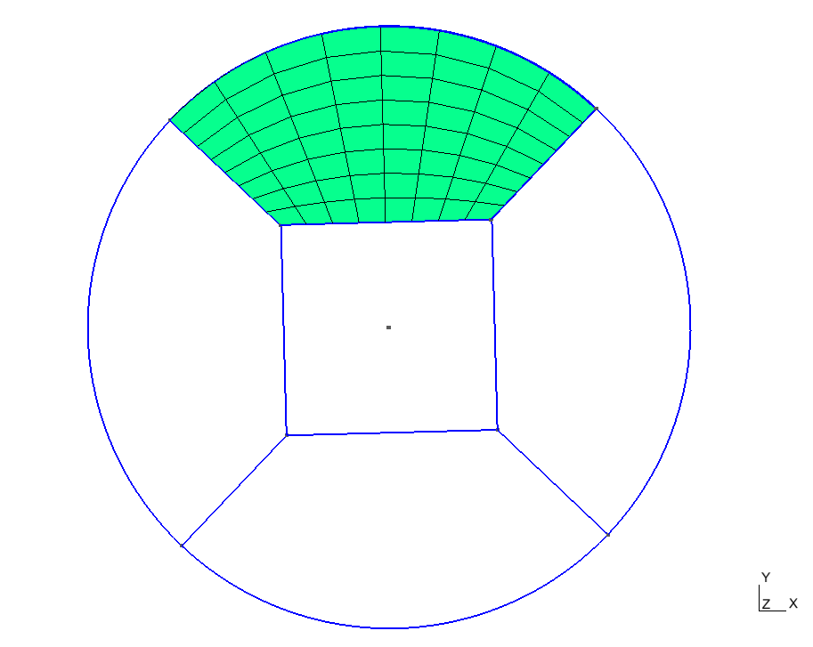
Figure 4.2. Macrocell approach: an example of a mesh made of five macrocells. Each macrocell is then split into several subcells. Only the subcells of the top macrocell are represented here (in green).

In schnaps we have also defined an interface structure in order to manage data communications between the macrocells. An interface contains the faces that are common to two neighboring macrocells. We do not proceed exactly as in Section 4.1 where the vertices of graph $\mathcal{G}$ were associated to cells and the edges to faces. Instead, we construct an upwind graph whose vertices are associated to macrocells, and edges to interfaces. This graph is then sorted, and the macrocells are numbered in a topological order.

For solving one time step of one transport equation (4.2), we split the computations into several elementary operations: for all macrocell $\mathcal{L}$ taken in a topological order, we perform the following tasks:

1. Volume residual assembly: this task computes in the macrocell $\mathcal{L}$ the part of the right hand side of (4.2) that comes from the values of $f$ inside $\mathcal{L}$;

2. Interface residual assembly: this task computes, in the macrocell $\mathcal{L}$, the part of the right hand side of (4.2) that comes from upwind interface values;

3. Boundary residual assembly: this task computes, in the macrocell $\mathcal{L}$, the part of the right hand side of (4.2) that comes from upwind boundaries values.

4. Volume solve: this task solves the local transport linear system in the macrocell.

5. Extraction: this task copies the boundary data of $\mathcal{L}$ to the neighbor downwind interfaces.

Let us point out that in step 4 above, the macrocell local transport solver is reassembled and refactorized at each time step: we have decided not to store a sparse linear system in the macrocell for each velocity $\mathbf{v}_{i}$, in order to save memory. The local sparse linear system is solved thanks to the KLU library [5]. This library is able to detect efficiently sparse triangular matrix structures, which makes the resolution quite efficient. In practice, the factorization and resolution time of the KLU solver is of the same order as the residual assembly time.

In schnaps, we use the MPI version of StarPU. The macromesh is initially split into several subdomains and the subdomains are distributed to the MPI nodes. Then the above tasks are launched asynchronously with the starpu_mpi_insert_task function. MPI communications are managed automatically by StarPU.

It is clear that if we were solving a single transport equation our strategy would be very inefficient. Indeed, the downwind subdomains would have to wait for the end of the computations of the upwind subdomains. We are saved by the fact that we have to solve many transport equations in different directions. This helps the MPI nodes to be equally occupied. Our approach is more efficient if we avoid a domain decomposition with internal subdomains, because these subdomains have to wait the results coming from the boundaries.

In our approach it is also essential to launch the tasks in a completely asynchronous fashion. In this way, if a MPI node is waiting for results of other subdomains for a given velocity $\mathbf{v}_{i}$ it is not prevented from starting the computation for another velocity $\mathbf{v}_{j}.$

4.4. Collisions

In this section we explain how is computed the collision step (3.12). The computations are purely local to each GL point, which makes the collision step embarrassingly parallel. However it is not so obvious to attain high efficiency because of memory access. If the values of $\mathbf{F}$ are well arranged in memory in the transport stage, it means that the values of $\mathbf{{f}}$ attached to a given velocity $\mathbf{v}_{i}$ are close in memory, for a better data locality. On the contrary, in the collision step at a given GL point, a better locality is achieved if the values of $\mathbf{{f}}$ corresponding to different velocities are close in memory. Additional investigations and tests are needed in order to evaluate the importance of data locality in our algorithm.

In our implementation, we have adopted the following strategy. We have first identified the following task:

1. Reduction task for a velocity $\mathbf{v}_{i}$: this task is associated with one macrocell $\mathcal{L}$. It computes the contribution to $\mathbf{w}$ of the components of $\mathbf{f}$ that have been transported at velocity $\mathbf{v}_{i}$ with formula (2.2). The StarPU access to the buffer containing $\mathbf{w}$ is performed in read-write and commute modes. In this way the contribution from each velocity can be added to $\mathbf{w}$ as soon as it is available.

2. Relaxation task for a velocity $\mathbf{v}_{i}$: this task is associated to one macrocell $\mathcal{L}$. Once $\mathbf{w}$ is known, it computes the components of $\mathbf{{f}}^{eq}$ corresponding to velocity $\mathbf{v}_{i}.$ Then it computes the relaxation step (3.12) for the associated component of $\mathbf{f}$.

In step 2 we can separate the computations for each velocity because the collision term (3.10) is diagonal. Some Lattice Boltzmann Methods rely on non-diagonal relaxations. It can be useful for representing more general viscous terms for instance. For non-diagonal relaxation we would have to change a little the algorithm.

We can now make a few comments about the storage cost of the method. In the end, we have to store at each GL point $\mathbf{x}_{i}$ and each cell $L$ the values of $\mathbf{{f}}_{L,i}$ and $\mathbf{w}_{L,i}$. We do not have to keep the values of the previous time-step, $\mathbf{{f}}_{L,i}$ and $\mathbf{w}_{L,i}$ can be replaced by the new values as soon as they are available. In this sense, our method is “low-storage”. As explained in [4] it is also possible to increase the time order of the method, without increasing the storage.

4.5. Scaling test

For all performance tests presented in this section, we used standard models from the family Lattice-Boltzmann-Method (LBM) kinetic models devised for the simulation of Euler/Navier Stokes systems. We will not give a detailed description of their properties from the modeling point of view: we simply take them as good representative of the typical workload of kinetic relaxation schemes. The most relevant feature impacting the performance of our algorithm is the discrete velocity set of the kinetic model, which determines the task graph structure of the transport step when combined with a particular mesh topology. In standard LBM models, velocity sets are usually built-up from a sequence of pairs of opposite velocities with an additional zero velocity node. On Figure 4.3 we show the two representative velocity sets of the $2DQ9$ and $3DQ27$ LBM models.

Figure 4.3. D2Q9 and D3Q27 velocity grids.

4.5.1. Multithread performance (D2Q9, D3Q*)

We first tested the multithread performance of our implementation for the full (transport + relaxation) scheme for the standard D2Q9 model. All tests were performed on a single node of the IRMA-ATLAS cluster, with 24 available cores. We considered several square meshes build-up from 1 to 64 macrocells. The number of geometric degrees of freedom per element has been kept constant with a value of $3375$ points per macrocell, so that the workload per macrocell did not change. For each mesh, we allowed StarPu to use from 1 to the full 24 cores of the node and measured the total wall time. The results for this first batch of performance measurements are given in Fig. 4.4. First we verify that for 1 unique macrocell, parallel performance saturates when the number of cores roughly equals the number of velocities in the model. This is to be expected, as no topological parallelism can be exploited in that case. Increasing the number of macro-element allows to take advantage of topological parallelism. For that workload, parallel efficiency saturates at about $80$, which is quite good. On Fig. 4.5, we considered on the same cubic mesh three different models differing by the number of velocity values. Those cases exhibit a large amount of potential parallelism, due to the large number of velocities combined with the macrocell decomposition. On an ideal machine, they could in theory scale perfectly up to 24 cores. The observed saturation, still around $80$ efficiency, is still quite good and comes from the unavoidable concurrency in memory access between the various cores and the scheduling overhead. It is important to note when considering those results that the bulk of the computational cost occurs in the transport step of the algorithm: though the collision step forces synchronization between all the fields corresponding to individual velocities for the computation of the macroscopic fields, its actual cost is negligible in regard of the transport step.

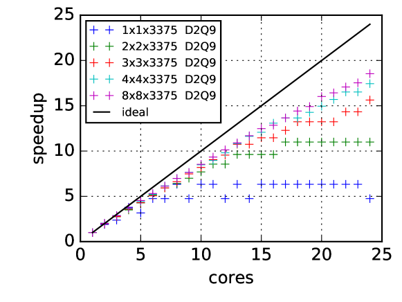
Figure 4.4. Multithread scaling for the D2Q9 model and a collection of square meshes from 1 to 64 macro-elements.

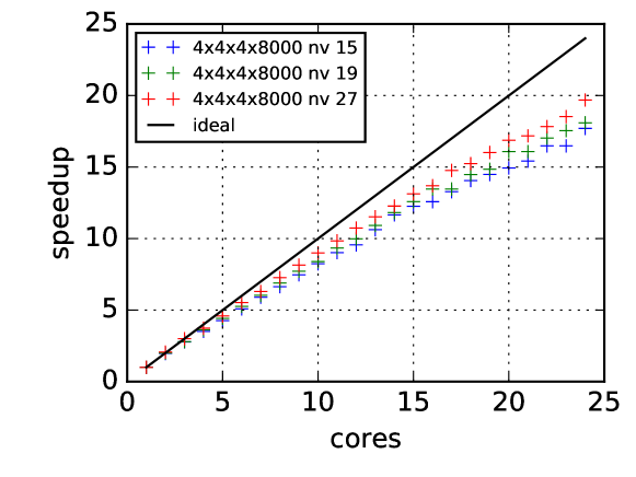
Figure 4.5. Multithread scaling on a 4x4x4 macro-element mesh for models D3Q15, D3Q19 and D3Q27

4.5.2. MPI scaling: D3Q15 in a torus

Having verified the good multithread performance of our code on a single node, we now check whether for larger problem sizes the workload can be distributed among several computing nodes. To that end, accounting for the fact that we aim notably at performing simulations for Tokamak physics, we considered a toroidal mesh subdivided into $720$ macrocells. The workload distribution across nodes was made using a standard domain decomposition approach: the mesh was partitioned statically into as many sub-domains as computing nodes, ranging from $1$to $4$ for our experiment on the IRMA-ATLAS cluster. From an implementation point of view, the transition from a multithreaded code to a hybrid MPI/multithread one is made fairly easy by StarPU. When declaring data to StarPU, one simply has to specify the MPI process owning the data. At runtime, each MPI process hosts a local scheduler instance which acts only on data relevant to the local execution graph. All MPI communications are handled transparently by the local scheduler when inter-node data transfers are necessary. In table 1 we show the wall time for a hundred iterations of the full scheme for the D3Q15 model. The number of available threads per node was set to $14,$ matching the number of velocities actually participating in transport (there is one null velocity in the model). We observe a super-linear scaling when the load is spread from $1$to $4$ node. This is not surprising for such an experiment with fixed total problem size as both the memory load and size of the local task graph for each decrease when the number of sub-domains increases.

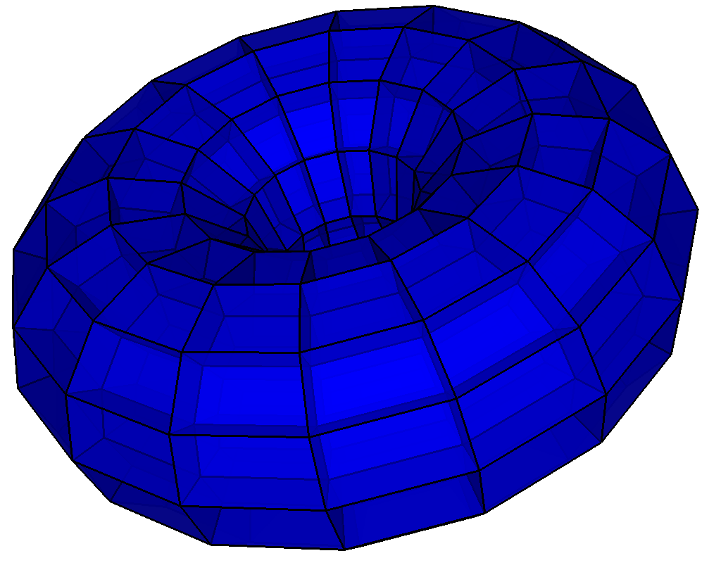
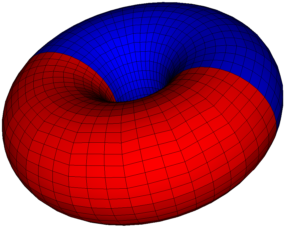
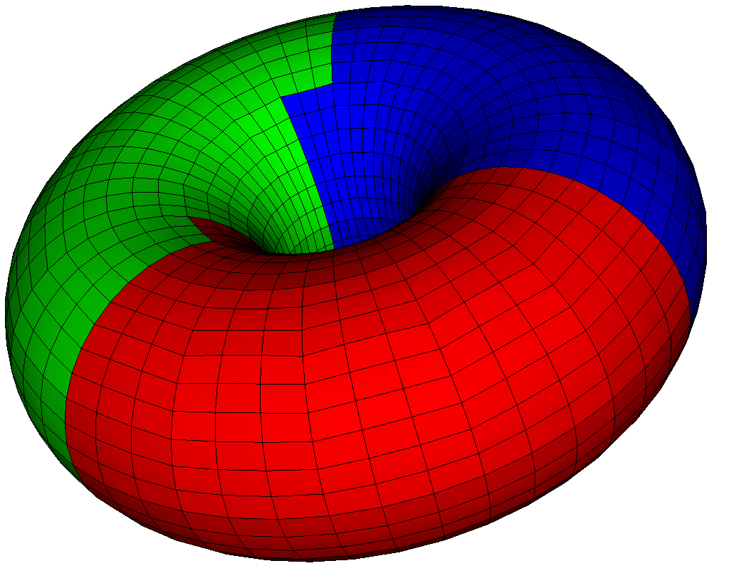
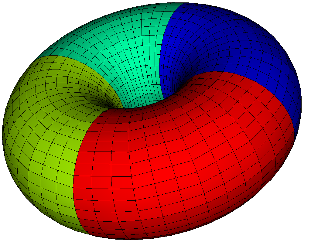
Figure 4.6. Toroidal macromesh ($720$ macrocells) - Mesh partitions used in the MPI scaling tests.

Nthreads/Nmpi	1	2	3	4
14	6862	2772	1491	1014

Table 1. Wall time (in seconds) for the D3Q15 model for 1 to 4 mpi processes with 14 threads per process.

5. Numerical results

5.1. Euler with gravity

For this test case we consider the isothermal Euler equations in two dimensions with a constant gravity source term

(5.1) $$\partial_{t}\rho+\partial_{k}(\rho\mathbf{\mathbf{u}^{k})}=0,$$

(5.2) $$\partial_{t}(\rho\mathbf{u}^{k})+\partial_{j}\boldsymbol{\Pi^{kj}}=\rho\mathbf{g},$$

with $\boldsymbol{\Pi}=\left[\begin{array}[]{cc}\rho c^{2}+\rho u_{x}^{2}&\rho u_{x}u_{y}\\ \rho u_{x}u_{y}&\rho c^{2}+u_{y}^{2}\end{array}\right]$ and $\mathbf{g}=-g\mathbf{e}_{y}$.

The conservative variables vector is thus $\mathbf{w}=[\rho,\rho u_{x},\rho u_{y}]^{t}$ . The kinetic model is the standard $D2Q9$ one with nine velocities

(5.3) $$\mathbf{V}=\lambda\mathrm{\textrm{diag}}\left[(0,0),(1,0),(0,1),(-1,0),(0,-1),(1,1),(-1,1),(-1,-1),(1,-1)\right]$$

and the $(3\times 9)$ projection matrix $P$ reads

(5.4) $$P=\begin{bmatrix}1&1&1&1&1&1&1&1&1\\ 0&\lambda&0&-\lambda&0&\lambda&-\lambda&-\lambda&\lambda\\ 0&0&\lambda&0&-\lambda&\lambda&\lambda&-\lambda&-\lambda\end{bmatrix},$$

i.e $\rho=\sum_{i}f_{i}$, $\rho\mathbf{u}=\sum_{i}f_{i}\mathbf{v}_{i}$.

The equilibrium distribution function is given by

(5.5) $$f_{i}=w_{i}\rho\left(1+\frac{(\mathbf{u}\cdot\mathbf{v}_{i})}{c^{2}}+\frac{(\mathbf{u}\cdot\mathbf{v}_{i})^{2}}{2c^{4}}-\frac{\mathbf{u}\cdot\mathbf{u}}{2c^{2}}\right)$$

with $c=\lambda/\sqrt{3}$, and the weights $w_{0}=\frac{4}{9}$, $w_{i}=\frac{1}{9}$ for $i=1,\dots,4$, $w_{i}=\frac{1}{36}$ for $i=5,\dots,8$.

The stationary solution for a fluid at rest in the gravity field is

(5.6) $$\rho=\rho_{0}\exp(-gy/c^{2}),\qquad\mathbf{u}=0$$

For this test case, the numerical scheme is made up of three stages: a transport step (T), a source step (S) where the source is applied on the equilibrium part of the distribution function, and the collision step (C). Due to the absence of explicit time dependency and the linearity in $\mathbf{w}$ of the source, the local nonlinear resolution of the source operator converges in one Picard iteration. All steps are implemented as weighted implicit schemes, parametrized by a weight $\theta$ and a time step$\Delta t$.

We compared several $1^{st}$ and $2^{nd}$ order splitting schemes built up from either fully implicit ($\theta=1$) first order or Crank-Nicolson ($\theta=\frac{1}{2}$) steps:

• Lie first order splitting scheme $M_{1}^{s}=T_{1}(\Delta t)$$S_{1}(\Delta t)$$C_{1}(\Delta t)$ with first order building blocks.

• Lie first order splitting scheme $M_{1,2}^{s}=T_{2}(\Delta t)$$S_{2}(\Delta t)$$C_{2}(\Delta t)$ with second order building blocks, for which the order loss comes from the splitting error.

• a palindromic second order Strang scheme $M_{2}^{s}=T_{2}(\frac{\Delta t}{2})$$S_{2}(\frac{\Delta t}{2})$$C_{2}(\Delta t)$$S_{2}(\frac{\Delta t}{2})$$T_{2}(\frac{\Delta t}{2})$ .

• a collapsed version of the second order Strang scheme $M_{2}^{s}$for which the last transport substep of each global step and the first transport substep of the next one are fused in a single $T_{2}(\Delta t)$ substep except obviously for the first and last time steps of the simulation.

We performed time order convergence tests on a $2D$ square mesh partitioned into $4\times 4$ macrocells with $1024$ points per macrocell. As shown by Fig. 5.1, we obtain the expected convergence orders for each of the splitting schemes used.

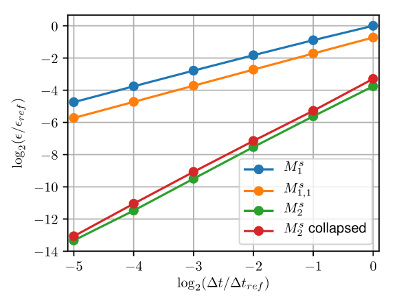
Figure 5.1. Time order convergence for the $2D$ Euler gravity test case with $D2Q9$ model. Convergence is estimated using the relative $L^{2}$ error $\epsilon$ on macroscopic variables with respect to the analytical solution at $t_{max}\approx 0.12$. The reference values $(\Delta t_{ref},\epsilon_{ref})$ of the logarithmic scale are $\Delta t_{ref}=0.024,\epsilon_{ref}=0.0143$.

5.2. 2D Flow around a cylinder using a penalization method

In this test case we considered the flow of a fluid in a rectangular duct with a cylindrical solid obstacle. The simulation domain is the rectangle $[-1,1]\times[-5,5]$

The effect of the obstacle on the flow is modeled using a volumic source term of the form

(5.7) $$\mathbf{{s}}=K(\mathbf{x})(\mathbf{w}-\mathbf{w}_{s}),$$

with $\mathbf{w}_{s}=[1.0,0,0]^{t}$ the target fluid state in the “solid” part of the domain and the relaxation frequency $K(\mathbf{x})$ is given by

(5.8) $$K(\mathbf{x})=K_{s}\exp(-\kappa(\mathbf{x}-\mathbf{x}_{c})^{2}),$$

with $\text{$K_{s}=300$, }\mathbf{x}_{c}=[-4,0]^{t}$and $\kappa=40$. The net effect is a very stiff relaxation towards a flow with zero velocity and the reference density near the center $\mathbf{x}_{c}$ of the frequency mask. The effective diameter of the cylinder for this simulation is about $0.5$. The initial state, which is also applied at the duct boundaries for the whole simulation is $\rho=1,u_{x}=0.03,u_{y}=0$. Accounting for the fact that for this model the sound speed is $1/\sqrt{3}$, the Mach number of the unperturbed flow is approximately $0,017$. The simulation was performed on a macromesh with $16\times 16$ macrocells stretched with a $1:5$ aspect ratio to match the domain dimension; each macrocell contains $12\times 60$ integration points. On figure 5.2 we show the vorticity norm at $t=83$, when turbulence is well developed in the wake of the obstacle.

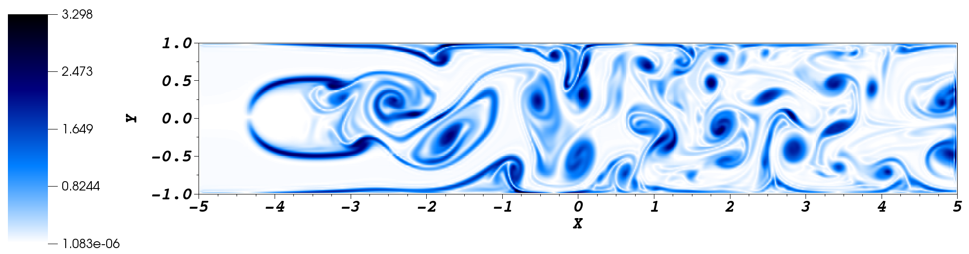
Figure 5.2. . Flow around cylindrical obstacle. Vorticity norm $|\nabla\times u|$ at $t=83$, showing the turbulent field behind the obstacle.

6. Conclusion

In this paper, we have presented an optimized implementation of the Palindromic Discontinuous Galerkin Method for solving kinetic equations with stiff relaxation. The method presents the following interesting features:

• It can be used for solving any hyperbolic system of conservation laws.

• It is asymptotic-preserving with respect to the stiff relaxation.

• It is implicit and thus is not limited by CFL conditions.

• Despite being formally implicit, it requires only explicit computations.

• It is easy to increase the time order with a composition method.

• It presents many opportunities for parallelization and optimization: in this paper we have presented the parallelization of the method with the aid of the MPI version of the StarPU runtime system. In this way we address both shared memory and distributed memory MIMD parallelism.

Our perspectives are now to apply the method for computing MHD instabilities in tokamaks. We will also try to extend the method to more general boundary conditions.

References

- [1] Denise Aregba-Driollet and Roberto Natalini. Discrete kinetic schemes for multidimensional systems of conservation laws. SIAM Journal on Numerical Analysis, 37(6):1973–2004, 2000.
- [2] Cédric Augonnet, Olivier Aumage, Nathalie Furmento, Raymond Namyst, and Samuel Thibault. StarPU-MPI: Task Programming over Clusters of Machines Enhanced with Accelerators. In Siegfried Benkner Jesper Larsson Träff and Jack Dongarra, editors, EuroMPI 2012, volume 7490 of LNCS. Springer, September 2012. Poster Session.
- [3] François Bouchut, François Golse, and Mario Pulvirenti. Kinetic equations and asymptotic theory. Elsevier, 2000.
- [4] David Coulette, Emmanuel Franck, Philippe Helluy, Michel Mehrenberger, and Laurent Navoret. Palindromic discontinuous galerkin method for kinetic equations with stiff relaxation. arXiv preprint arXiv:1612.09422, 2016.
- [5] Timothy A Davis and Ekanathan Palamadai Natarajan. Algorithm 907: Klu, a direct sparse solver for circuit simulation problems. ACM Transactions on Mathematical Software (TOMS), 37(3):36, 2010.
- [6] Christophe Geuzaine and Jean-François Remacle. Gmsh: A 3-d finite element mesh generator with built-in pre-and post-processing facilities. International Journal for Numerical Methods in Engineering, 79(11):1309–1331, 2009.
- [7] Benjamin Graille. Approximation of mono-dimensional hyperbolic systems: A lattice boltzmann scheme as a relaxation method. Journal of Computational Physics, 266:74–88, 2014.
- [8] Ernst Hairer, Christian Lubich, and Gerhard Wanner. Geometric numerical integration: structure-preserving algorithms for ordinary differential equations, volume 31. Springer Science & Business Media, 2006.
- [9] Claes Johnson, Uno Nävert, and Juhani Pitkäranta. Finite element methods for linear hyperbolic problems. Computer methods in applied mechanics and engineering, 45(1):285–312, 1984.
- [10] Robert I McLachlan and G Reinout W Quispel. Splitting methods. Acta Numerica, 11:341–434, 2002.
- [11] Salli Moustafa, Mathieu Faverge, Laurent Plagne, and Pierre Ramet. 3d cartesian transport sweep for massively parallel architectures with parsec. In Parallel and Distributed Processing Symposium (IPDPS), 2015 IEEE International, pages 581–590. IEEE, 2015.