Interpolation between low and high temperatures of the specific heat for spin systems

Abstract

The high temperature expansion (HTE) of the specific heat of a spin system fails at low temperatures, even if it is combined with a Padé approximation. On the other hand we often have information about the low temperature asymptotics (LTA) of the system. Interpolation methods combine both kind of information, HTE and LTA, in order to obtain an approximation of the specific heat that holds for the whole temperature range. Here we revisit the entropy method that has been previously published and propose two variants that better cope with problems of the entropy method for gapped systems. We compare all three methods applied to the antiferromagnetic Haldane spin-one chain and especially apply the second variant, called Log Z method, to the cuboctahedron for different spin quantum numbers. In particular, we demonstrate that the interpolation method is able to detect an extra low-temperature maximum in the specific heat that may appear if a separation of two energy scales is present in the considered system. Finally we illustrate how interpolation also works for classical spin systems.

I Introduction

The Heisenberg model of interacting localized spins is an important canonical model for the theoretical study of quantum many-body systems rev1 ; rev2 . On the other hand, it provides an appropriate description of the properties of magnetic insulators rev1 ; rev2 . There are numerous theoretical methods to investigate the model. However, the theoretical description of highly frustrated quantum magnets is still a very challenging field of solid state theory. The powerful quantum Monte Carlo methods are severely limited in the presence of frustration due to the infamous “sign problem” TrWi05 ; rev2 . However, for systems in dimension $D=1$ the density-matrix renormalization group (DMRG) approach rev2 ; dmrg is very successful to deal with strongly frustrated quantum spin systems at zero and finite temperatures. The situation in $D>1$ is less satisfying. While for $T=0$ several effective approaches, such as the coupled-cluster method rev_ccm ; ccm2 , the functional renormalization group approach rev_fprg ; fprg , the exact diagonalization star04 ; ED40 ; lauchli2011 , the extension of the DMRG on $D=2$ DMRG_D2a ; DMRG_D2b or the tensor-network approach tensor are available, suitable methods for finite temperatures and $D>2$ in case of strong frustration are notoriously rare.

A universal method to investigate strongly frustrated quantum magnets is the high-temperature expansion domb_green ; OHZ06 . The roots of this method go back to a paper of W.  Opechowski published in 1937 opechowski . In the 1950ies and 1960ies the method was further developed and widely applied to various Heisenberg systems, see, e.g., Refs. wood1955, ; wood1958, ; wood1967, ; dalton1969, . At that time typically the HTE series for specific models could be calculated until order seven. In 1990ies an enormous progress calculating the HTE series for the Heisenberg model on various lattices could be achieved by using computer algebraic methods. Thus, for the frustrated triangular, kagome and hyperkagome lattices with only nearest-neighbor exchange bonds for spin quantum number $s=1/2$ the HTE series is available up to 14th (16th) order for the triangular (kagome and hyperkagome) lattice elstner1993 ; elstner1994 ; singh2012 . However, often we face more complicated systems with more than one exchange parameter. To determine the HTE series is then more ambitious, since more complex graphs on the lattice have to be taken into account. As a result, available series for more complicated models are limited to lower orders 2DJ1J2 ; Kapellasite . Another difficulty limiting the order of the series arises for higher spin quantum numbers $s>1/2$, because the HTE series of order $n$ contains $n$th-order polynomials in $s(s+1)$ which have to be determined for each model separately. On the other hand, more complex models as well as higher spin quantum numbers are relevant for many frustrated magnetic compounds, see, e.g., Refs. 2DJ1J2, ; Kapellasite, ; s1, ; s32, . Bearing in mind the universal character of the HTE approach it is desirable to have a general HTE tool to generate the series for Heisenberg models with arbitrary exchange patterns and arbitrary spin quantum number $s$. An early attempt to provide such a tool was published in Ref. SSL01, , where general analytical HTE expressions up to order three were given. Very recently some of the present authors have extended this general HTE scheme up to 10th order HTE_wir . The 10th order scheme is encoded in a simple C++-program and can be downloaded url_HTE10 and freely used by interested researchers. The ‘raw’ 10th order HTE series provide a good description of thermodynamic quantities down to about $1.5J$, where $J$ is a characteristic exchange energy of the spin model HTE_wir . The region of validity of the HTE can be significantly extended by Padé approximants baker61 (see also Refs. domb_green, and OHZ06, ). The Padé approximants are ratios of two polynomials $[m,n]=P_{m}(x)/R_{n}(x)$ of degree $m$ and $n$ and they provide an analytic continuation of a function $f(x)$ given by a power series. Such Padé approximants may yield reasonable data down to about $0.5J$.

Having in mind that often we have information on ground-state (and low-energy) properties obtained by special techniques designed for this purpose, see above, there remains a gap between the low-temperature description $T\ll J$ and the Padé-HTE description at $T\gtrsim 0.5J$. This gap is particularly relevant for strongly frustrated magnets, since the new state of matter in these system appear at temperatures well below $J$. To bridge this gap, a sophisticated interpolation procedure based on exploiting sum rules constraining the specific heat was proposed in Refs. BM01, and MB05, , henceforward called the “entropy method". Together with the general 10th HTE scheme the interpolation scheme may present a quite universal and powerful instrument to study the specific heat of frustrated quantum magnets and to provide model data to compare with experimental results.

To demonstrate this is an aim of the present paper. Another motivation to reinvestigate the entropy method of Bernu and Misguich BM01 ; MB05 and to propose alternative interpolation schemes consists in the following: (i) As for the HTE itself also for the interpolation Padé approximants are used. Often it happens that these approximants exhibit unphysical poles at temperatures in the region of interest. Having various interpolation schemes at hand one can simply exclude such an approximant present in one scheme but absent in another one. (ii) For spin systems with an excitation gap $\Delta$ (that is a a quite common property of systems with a quantum paramagnetic ground state) the approach of Bernu and Misguich is based on the special ansatz $c(T)\sim A\;T^{-2}e^{-\Delta/T}$ for the low-temperature behavior of the specific heat which might be not the correct one for the considered gapped spin system. One example is the Haldane spin-one antiferromagnetic spin chain, where this special ansatz has to be replaced by $c(T)\sim A\;T^{-3/2}e^{-\Delta/T}$.

The entropy method is based on the idea not to interpolate the specific heat $c(T)$ directly but rather the entropy $s$ considered as a function $s(e)$ of the energy $e$ utilizing the behavior of $s(e)$ for the two limits of low and high temperatures. The first modification of this method consists of representing the graph of $s(e)$ in parametric form as $s(\beta)$ and $e(\beta)$ where $\beta=1/T$ and to interpolate both parametrizations separately. This gives the “modified entropy method" that avoids the mentioned problem with the LTA ansatz.

Another alternative, still in the spirit of the entropy method, is based on the interpolation of $\ell(\beta)\equiv\log Z(\beta)$ where $Z$ denotes the partition function or rather its thermodynamic limit. The present paper focuses on this method, called the “Log Z method". It works for rather general LTA including finite spin systems and classical ones.

The paper is organized as follows. First we sketch the basic ideas underlying the various interpolation schemes. In section II we explain what we will call “pure interpolation" using a toy example. The specific heat satisfies two integral constraints or “sum rules". Interpolation with constraints, to be considered in section III, proceeds by pure interpolation of another thermodynamic function and by deriving $c(T)$ from this function. This function will be $s(e)$ for the entropy method, subsection III.1, or the functions $s(\beta)$ and $e(\beta)$ for the modified entropy method, subsection III.2, or the function $\ell(\beta)$ for the Log Z method, subsection III.3.

The next section IV contains tests and applications. First, in subsection IV.1, we revisit the example already considered in BM01 , the $s=1$ Haldane chain, and show that all three methods yield comparable results despite the different forms of the LTA. The second subsection IV.2 is devoted to the cuboctahedron and the Log Z method. This is a finite spin system that can be numerically exactly solved for $s=1/2$, $s=1$, and $s=3/2$ and thus serves as a test for the considered interpolation scheme. In particular, we want to find out whether an additional low-temperature maximum present in $c(T)$ for $s=1/2$ and $s=1$ can be detected by the interpolation scheme. For higher $s$, where no exact data are available, the Log Z method yields predictions about the form of $c(T)$ for low and intermediate temperatures that are hardly available by other methods. Finally, in section V, we extend the range of applications to classical spin systems where a modified second integral constraint has to be considered. We conjecture that the LTA of the specific heat has a similar form as for gapped quantum systems and verify this conjecture in subsection V.1 for the special case of the classical equilateral spin triangle that can be solved analytically. In the appendix A we show how to derive the LTA of the classical spin triangle without using the analytical solution.

II Pure interpolation

To illustrate the basic ideas of the interpolation we consider a toy example. Let the error function $\mbox{erf}(\beta)$ be the unknown thermodynamical function, where $\beta$ is the inverse temperature, and assume that we know a finite number of terms of its high temperature expansion (HTE)

$$\mbox{erf}(\beta)=\frac{2}{\sqrt{\pi}}\beta-\frac{2}{3\sqrt{\pi}}\beta^{3}+\ldots\;,$$ (1)

as well as its low-temperature asymptotic (LTA)

$$\mbox{erf}(\beta)\sim\mbox{erf}_{\infty}(\beta)\equiv 1-\frac{e^{-\beta^{2}}}{\sqrt{\pi}\beta}\;,\quad\beta\rightarrow\infty\;.$$ (2)

The LTA of a thermodynamic function will always be indicated by the subscript $\infty$ reminding that this is the case of $\beta\rightarrow\infty$. The basic idea of interpolation is to multiply the LTA by a Padé approximant, e. g.,

$$\mbox{erf}_{\mbox{\scriptsize int}}(\beta)=\mbox{erf}_{\infty}(\beta)\frac{a_{0}+a_{1}\beta+a_{2}\beta^{2}}{1+a_{3}\beta+a_{2}\beta^{2}}\;.$$ (3)

We have chosen the same coefficient $a_{2}$ for the leading coefficient of the numerator and the denominator of the Padé approximant in order to guarantee $\mbox{erf}_{\mbox{\scriptsize int}}(\beta)\rightarrow\mbox{erf}_{\infty}(\beta)$ for $\beta\rightarrow\infty$. Further we have to choose the coefficients $a_{0},\ldots,a_{3}$ such that the HTE of $\mbox{erf}_{\mbox{\scriptsize int}}(\beta)$ coincides with the known HTE of $\mbox{erf}(\beta)$ up to $3$rd order. Here we face a problem that is typical for the interpolation of thermodynamical functions, namely that $\mbox{erf}_{\mbox{\scriptsize int}}(\beta)$ is not analytical at $\beta=0$ due to the factor $\frac{1}{\beta}$ in (2). Hence one could not calculate its HTE as required by the method.

There are different ways to cope with this problem. The first one is to modify the Padé approximant such that $\mbox{erf}_{\mbox{\scriptsize int}}(\beta)$ becomes analytical and to write

$$\mbox{erf}_{\mbox{\scriptsize int}}(\beta)=\mbox{erf}_{\infty}(\beta)\frac{a_{1}\beta+a_{2}\beta^{2}}{1+a_{3}\beta+a_{2}\beta^{2}}\;.$$ (4)

The Padé approximant has now a series expansion that starts with $a_{1}\beta$ and cancels the disturbing factor $\frac{1}{\beta}$. In our toy example we would then have to determine four unknown coefficients and need the HTE of erf up to third order.

Another way out especially employed in BM01 is the use of auxiliary functions. In our case the function

$$G(\beta)\equiv(1-\mbox{erf}_{\infty}(\beta))^{-1}=\sqrt{\pi}\,\beta\,\exp(\beta^{2})\;,$$ (5)

is analytical at $\beta=0$ and the corresponding interpolation ansatz reads

$$G_{\mbox{\scriptsize int}}(\beta)=\sqrt{\pi}\,\beta\,\exp(\beta^{2})\frac{a_{0}+a_{1}\beta+a_{2}\beta^{2}}{1+a_{3}\beta+a_{2}\beta^{2}}\;.$$ (6)

The rest is analogous to the above procedure; we choose $a_{0},a_{1},a_{2}$ such that the HTE of $G_{\mbox{\scriptsize int}}(\beta)$ coincides with the known HTE of $(1-\mbox{erf}(\beta))^{-1}$ up to second order. Of course, one has to solve the result for $\mbox{erf}_{\mbox{\scriptsize int}}$. It is not necessary to provide the further details of the toy example. It turns out that already the second order of HTE is sufficient to obtain a reasonably good interpolation of the erf function. But this is obviously due to the smooth behavior of erf between the low- and the high-temperature regime. The specific heat has one or even two maxima for intermediate temperatures and thus represents a greater challenge for interpolation.

By the second method we can also treat the case where some constants in the LTA are unknown. Assume, for example, that we only know that the LTA of erf is of the form

$$\mbox{erf}(\beta)\sim\mbox{erf}_{\infty}(\beta)\equiv 1-A\frac{e^{-\beta^{2}}}{\beta}\;,\quad\beta\rightarrow\infty\;.$$ (7)

In this case we would replace (6) by

$$G_{\mbox{\scriptsize int}}(\beta)=\beta\,\exp(\beta^{2})\frac{a_{0}+a_{1}\beta+a_{2}\beta^{2}}{1+a_{3}\beta+a_{4}\beta^{2}}\;,$$ (8)

and determine $A$ by the ration $a_{2}/a_{4}$ as a by-product of the Padé approximation. In what follows we refer to the above illustrated scheme as pure interpolation.

III Interpolation with constraints

As mentioned in the Introduction the task of interpolating the specific heat becomes more difficult if we try to allow for the two integral constraints

$$\int_{0}^{\infty}c(T)dT = \int_{T=0}^{T=\infty}de=e_{\infty}-e_{0}=|e_{0}|,$$ (9)

$$\int_{0}^{\infty}\frac{c(T)}{T}dT = \int_{T=0}^{T=\infty}ds=s_{\infty}-s_{0}=\log(2s+1),$$ (10)

where we have assumed that the entropy $s_{0}$ of the ground state vanishes. On the other hand the interpolation becomes more accurate by taking into account this information. The basic idea of BM01 is to reduce the task of interpolation with constraints to a pure interpolation of the function $s=s(e)$. Hence this method has been dubbed the “entropy method". We will shortly recapitulate it following the ideas of Bernu and Misguich BM01 ; MB05 in the next subsection and then sketch two extensions, the “modified entropy method" and the “ log Z method".

III.1 The entropy method

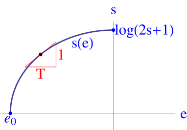
Figure 1: Typical graph of the function $s=s(e)$. The slope is the inverse temperature $\beta=\frac{1}{T}$ due to the Clausius formula $ds=\frac{de}{T}$.

For a spin system the graph of the function $s=s(e)$ typically has the form shown in Fig. 1. It is limited by the points $(s=0,e=e_{0})$ and $(s=\log(2s+1),e=0)$ corresponding to $T=0$ and $T=\infty$. Since

$$\frac{d\,s}{d\,e}=\beta=\frac{1}{T}\;,$$ (11)

the slope of the graph vanishes at $T=\infty$ and diverges at $T=0$. The specific heat $c=c(e)$ can be obtained by

$$\frac{1}{c(e)} = \frac{d\,T}{d\,e}=\frac{d}{d\,e}\left(\frac{d\,s}{d\,e}\right)^{-1}=-\frac{s^{\prime\prime}(e)}{s^{\prime}(e)^{2}}\;,$$ (12)

$$c(e) = -\frac{s^{\prime}(e)^{2}}{s^{\prime\prime}(e)}\;.$$ (13)

The entropy method assumes that we know the HTE and the LTA of $s(e)$. Whereas the HTE can be derived from that of $c(\beta)$ without problems, the derivation of an explicit LTA may be problematic as we will see below. But if we assume the HTE and LTA of $s(e)$ as given we may perform a pure interpolation by one of the methods sketched in section II and obtain some approximation $s_{\mbox{\scriptsize int}}(e)$ of $s(e)$. From this we obtain the corresponding $c_{\mbox{\scriptsize int}}(e)$ by (13) and $\beta_{\mbox{\scriptsize int}}(e)$ by (11). The plot of the final result $c=c_{\mbox{\scriptsize int}}(\beta)$ can be obtained in parametric form from these results or by inserting the numerically obtained inversion of $\beta_{\mbox{\scriptsize int}}(e)$. It necessarily satisfies the integral constraints (9), (10) and has the correct behavior for low and high temperatures.

In the applications of the interpolation method we find three cases of the LTA of the specific heat, namely

$$c(T) \sim A\;T^{\alpha}\;,$$ (14)

$$c(T) \sim A\;T^{\alpha}e^{-\Delta/T}\;,$$ (15)

$$c(T) \sim T^{-2}\sum_{\nu=1}^{n}d_{\nu}\delta_{\nu}^{2}e^{-\delta_{\nu}/T}.$$ (16)

The case (14) occurs for gapless systems, (15) for systems with an energy gap $\Delta$ and (16) for finite systems. The latter case will be considered in more details in section III.3 where also the notation will be explained. The entropy method applies to the cases (14) and (15), where the latter case has to be restricted to $\alpha=-2$. Moreover, the case (16) with $n=1$ could be treated by this method. In the other cases one has the problem to find an explicit form of the LTA of $s(e)$. This is a motivation to extend the entropy method in order to cover all cases.

III.2 The modified entropy method

The crucial object of the entropy method is the graph of $s=s(e)$. It can also be represented in parametric form by two functions $e=e(\beta)$ and $s=s(\beta)$. Here we have chosen the inverse temperature $\beta$ as the natural parameter; but sometimes it can be more convenient to choose other parameters such as $\sqrt{\beta}$ and to adapt the modified entropy method to this choice. We assume that for both functions $e=e(\beta)$ and $s=s(\beta)$ a pure interpolation is possible. For example, in the case (15) we could obtain an LTA of $e=e(\beta)$ and $s=s(\beta)$ in the following way:

$$e_{\infty}(\beta) = e_{0}-\int_{\infty}^{\beta}c_{\infty}(x)\frac{dx}{x^{2}}=e_{0}-A\int_{\infty}^{\beta}x^{-\alpha}e^{-\Delta x}\frac{dx}{x^{2}}$$ (17)

$$= e_{0}+A\left(\frac{\beta^{-2-\alpha}}{\Delta}e^{-\Delta\beta}+\int_{\infty}^{\beta}\frac{2+\alpha}{\Delta}x^{-3-\alpha}e^{-\Delta x}\,dx\right)$$

$$\sim e_{0}+A\;\frac{\beta^{-2-\alpha}}{\Delta}e^{-\Delta\beta}\;,$$

$$s_{\infty}(\beta) = -\int_{\infty}^{\beta}c_{\infty}(x)\frac{dx}{x}=-A\int_{\infty}^{\beta}x^{-\alpha}e^{-\Delta x}\frac{dx}{x}$$ (18)

$$= A\left(\frac{\beta^{-1-\alpha}}{\Delta}e^{-\Delta\beta}+\int_{\infty}^{\beta}\frac{1+\alpha}{\Delta}x^{-2-\alpha}e^{-\Delta x}\,dx\right)$$

$$\sim A\;\frac{\beta^{-1-\alpha}}{\Delta}e^{-\Delta\beta}\;.$$

We have obtained this result by partial integration and taking only the terms with the highest power of $\beta$. It is clear from (17) that $e_{\infty}(\beta)$ cannot be solved for $\beta$ except for $\alpha=-2$, and hence the entropy method cannot be applied to gapped systems in the general case. For the modified entropy method it is not necessary to solve $e_{\infty}(\beta)$ for $\beta$ since we apply the pure interpolation procedure directly to $e(\beta)$ and $s(\beta)$. Hence this method can be also applied to gapped systems with $\alpha\neq-2$.

From the approximated graph given by the parametric representation $e_{\mbox{\scriptsize int}}(\beta)$ and $s_{\mbox{\scriptsize int}}(\beta)$ we can obtain the specific heat $c(\beta)$ by

$$c(\beta)=-\frac{\dot{s}^{2}\dot{e}}{\ddot{s}\dot{e}-\dot{s}\ddot{e}}\;.$$ (19)

Here the dot indicates the derivative w. r. t. $\beta$ and the result easily follows from (13) by the chain rule.

Applications of the modified entropy method will be presented in section IV.1. As a drawback of this method we note that it results in two different temperature concepts, namely $T_{1}=\frac{1}{\beta}$ and $T_{2}=\frac{\dot{s}}{\dot{e}}$ that only coincide for the correct graph. For the approximated graph there will be a slight difference between $T_{1}$ and $T_{2}$, especially at low temperatures. It remains open which temperature one should choose for the final result of $c(T)$; $T_{1}$ gives the best results for the behavior at high and low temperatures and $T_{2}$ exactly satisfies the integral constraints (9),(10).

III.3 The Log Z method

This method is based on the well-known fact that both functions, $s(\beta)$ and $e(\beta)$, can be derived from a single thermodynamic function, namely $\log Z=\log\mbox{Tr}\left(e^{-\beta H}\right)$ or, more precisely, its thermodynamic limit

$$\ell(\beta)\equiv\lim_{N\rightarrow\infty}\frac{1}{N}\log Z_{N}\;.$$ (20)

In fact,

$$e(\beta) = -\frac{d}{d\beta}\ell(\beta)\;,$$ (21)

$$c(\beta) = \beta^{2}\frac{d^{2}}{d\beta^{2}}\ell(\beta)\;,$$ (22)

$$f(\beta) = -\frac{1}{\beta}\ell(\beta)\;,$$ (23)

$$s(\beta) = \beta\left(e(\beta)-f(\beta)\right)\;.$$ (24)

If we can determine the correct behavior of $\ell(\beta)$ for low and high temperatures, we can perform a pure interpolation and obtain $\ell_{\mbox{\scriptsize int}}(\beta)$. Then the functions $e_{\mbox{\scriptsize int}}(\beta)$ and $s_{\mbox{\scriptsize int}}(\beta)$ defined by (21) and (24) will automatically inherit the correct low and high temperature behavior. It follows from Eqs. (21) and (24) that $c_{\mbox{\scriptsize int}}(\beta)$ defined by (22) satisfies the integral constraints (9),(10). Moreover, $c_{\mbox{\scriptsize int}}(\beta)$ also has the correct LTA and HTE of the considered order.

Let $c(\beta)=\sum_{n=0}^{\infty}d_{n}\beta^{n}$ be the HTE of the specific heat and $\ell(\beta)=\sum_{n=0}^{\infty}a_{n}\beta^{n}$ that of Log Z, then (22) implies that $a_{n}=\frac{d_{n}}{n(n-1)}$ for all $n=2,3,\ldots$. Further, $a_{0}=\lim_{N\rightarrow\infty}\frac{1}{N}\log\mbox{Tr}\,{\mathbbm{1}}=\log(2s+1)$ by the definition (20), and $a_{1}=\mbox{Tr}H=0$. Hence, from a known HTE series of the specific heat $c$ up to order $n_{\mbox{\scriptsize max}}$ follows the HTE of $\ell(\beta)$ up to the same order.

For the LTA we first consider a finite system with energy eigenvalues $e_{0},e_{1},e_{2},\ldots$ and the corresponding degeneracies $d_{0}=1,d_{1},d_{2},\ldots$. Of course, the limit $N\rightarrow\infty$ is ignored for finite systems. Set $\delta_{\nu}\equiv e_{\nu}-e_{0}$ for $\nu=1,2,\ldots$. We thus have

$$Z = e^{-\beta e_{0}}+d_{1}\,e^{-\beta e_{1}}+d_{2}\,e^{-\beta e_{2}}+\ldots$$ (25)

$$= e^{-\beta e_{0}}(1+d_{1}\,e^{-\beta\delta_{1}}+d_{2}\,e^{-\beta\delta_{2}}+\ldots)\;,$$ (26)

and hence

$$\log Z = -\beta e_{0}+\log\left(1+d_{1}\,e^{-\beta\delta_{1}}+d_{2}\,e^{-\beta\delta_{2}}+\ldots\right)$$ (28)

$$\sim -\beta e_{0}+\sum_{\nu=1}^{m}d_{\nu}e^{-\beta\delta_{\nu}}\;\mbox{for }\beta\rightarrow\infty\;,$$

where we have truncated the summation at $\nu=m$ such that $\delta_{m}<2\delta_{1}$. Otherwise we should have included the second term of the Taylor series $\log(1+x)=x-\frac{x^{2}}{2}+\ldots$. This result also yields the LTA of the specific heat in (16) by means of (22). Note that the term $-\beta e_{0}$ in (LABEL:CL4a) has the effect that the LTA of $e(\beta)$ as well as of $f(\beta)$ starts with the term $e_{0}$, as it is expected.

Now we will assume that also for an infinite gapped spin system the LTA of $\ell(\beta)$ is of the form

$$\ell_{\infty}(\beta)=-\beta e_{0}+\frac{A}{\Delta^{2}}\beta^{\alpha-2}e^{-\Delta\beta}\;,$$ (29)

where $e_{0}$ has to be redefined as the ground state energy per spin in the thermodynamic limit. The notation is chosen such that (15) is obtained as the leading term of the LTA of $c(\beta)$.

In the applications to lattice spin systems it may happen that only $\Delta$ is known but $A$ is unknown or that both, $\Delta$ and $A$, are unknown. Hence it is important to note that, like the entropy method, also the Log Z method is principally able to obtain estimates of these data via interpolation in the way indicated at the end of section II.

This finishes the general explication of the log Z method. Further details will be given in the following sections including applications to concrete systems.

IV Tests and applications

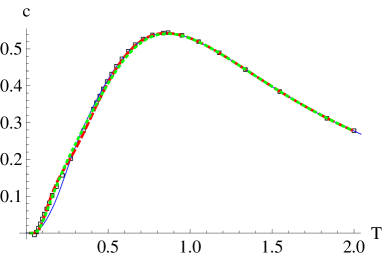
Figure 2: Comparison of the curves $c$ vs. $T$ for the $s=1$ Haldane chain determined by four different methods. The green dotted curve is obtained by the entropy method BM01 , the blue one by the modified entropy method, the red dashed one by the Log Z method, and the curve indicated by small black squares by DMRG methods, see X98 , Fig. 4.

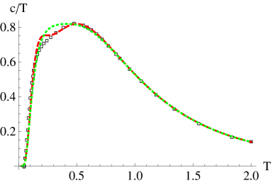
Figure 3: Comparison of the curves $c/T$ vs. $T$ for the $s=1$ Haldane chain determined by the following three different methods. The green dotted curve is obtained by the entropy method BM01 , the red one by the Log Z method, and the curve indicated by small black squares by DMRG methods, see X98 , Fig. 4.

IV.1 The $s=1$ Haldane chain

The $s=1$ antiferromagnetic Heisenberg spin chain (“Haldane chain") is an example of a gapped system where the LTA of the specific heat is known JG94 to be of the form

$$c_{\infty}(T)=\frac{\Delta^{5/2}}{\sqrt{2\pi}}T^{-3/2}e^{-\Delta/T}\;.$$ (30)

The values of the ground state energy $e_{0}=-1.401484038971(4)$ and the gap $\Delta=0.41050(2)$ have been determined by DMRG calculations WH93 . Also the specific heat has been calculated by these techniques that are especially suited for one-dimensional systems X98 . Hence this system can be used as a kind of test for interpolation methods.

Bernu and Misguich BM01 have applied the entropy method to the Haldane chain although the exponent in (30) is $\alpha=-3/2$ by simply setting $\alpha=-2$. They used unpublished HTE data up to the order 20 of Elstner, Jolicoeur, and Golinelli and an auxiliary function

$$G(e)=(e-e_{0})\frac{d}{de}\frac{s(e)}{e-e_{0}}\;.$$ (31)

By this they determined $\Delta$ by extrapolation w. r. t. the order $n$ approximately to $\Delta\approx 0.40$.

The modified entropy method and the Log Z method can be directly applied to the Haldane chain using the correct exponent $\alpha=-3/2$ of the LTA of $c(T)$. We have done this for both methods by using the same HTE data as BM01 . Since we are able to use the true exponent $\alpha=-3/2$, we use the full information about the gap and the prefactor of the LTA of the specific heat given above. We will explain some details of the procedure only for the Log Z method.

The LTA (30) is not analytic in $\beta$ due to the factor $\beta^{3/2}$. Instead of using an auxiliary function we will make a transformation to the independent variable $\gamma\equiv\sqrt{\beta}$. Hence our ansatz for the interpolation of $\ell(\gamma)$ assumes the form

$$\ell_{\mbox{\scriptsize int}}(\gamma) = -\gamma^{2}e_{0}+\sqrt{\frac{\Delta}{2\pi}}e^{-\Delta\gamma^{2}}\gamma^{-1}\,\times$$ (32)

$$\frac{a_{1}\gamma+\ldots+a_{2N}\gamma^{2N}}{1+a_{2N+1}\gamma+\ldots+a_{2N}\gamma^{2N}}\;.$$

Note that we have chosen the coefficients of the Padé function such that its numerator contains the factor $\gamma$ that cancels the $\gamma^{-1}$ of $\ell_{\infty}(\gamma)$. Moreover we can choose $2N=40$ since the HTE of $\ell(\gamma)$ is used up to the order $40$ w. r. t. $\gamma$. The final result has to be transformed back to the variable $\beta$.

We show the results of the three interpolation methods in Fig. 2 together with DMRG results obtained by X98 . The differences are rather small and only visible for low temperatures. The deviation at low temperatures of the curve corresponding to the modified entropy method from the other curves is probably due to the fact that it only uses HTE results up to $17$th order because of problems with spurious poles.

In order to better demonstrate the differences at low temperatures we have also plotted the results for $c/T$ vs. $T$ obtained by the entropy method BM01 , the Log Z method and the DMRG method X98 , see Fig. 3. The results according to the modified entropy method have not been included because of the larger deviations at low temperatures mentioned above. It appears that all three methods coincide in the large, although the two latter methods indicate the occurrence of a shoulder at $T\approx 0.2$, most markedly by the Log Z method. However, these findings do not favor one of the three interpolation methods and are rather suited for a positive test of consistency.

IV.2 The cuboctahedron

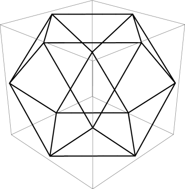
Figure 4: The cuboctahedron is an Archimedean solid that results from joining the $12$ midpoints of the edges of a cube.

Note first that in this section $\ell$ stands for the full Log Z (i.e. without division by $N$). The cuboctahedron is an Archimedean solid that results from joining the $12$ midpoints of the edges of a cube, see Fig. 4. It is an example of a finite spin system with $N=12$, where usually the spins are placed at the vertices and coupled to their nearest neighbors by the Heisenberg interaction model. For several reasons the investigation of the resulting Heisenberg model is an interesting problem. First of all, it is a paradigmatic model to study frustration effects schmidt2005 ; MCE2007 ; schnalle2009 ; honecker2009 ; dalton2010 ; Entel2011 ; Strecka2016 . Because the cuboctahedron is built by corner sharing triangles it can be considered as a finite-size relative of the celebrated kagome lattice, see, e.g., Refs. ccm2, ; lauchli2011, ; DMRG_D2a, ; DMRG_D2b, ; tensor, and references therein. For spin quantum numbers $s=1/2,1,\ldots,3$ the low-lying eigenstates of the quantum Heisenberg model were calculated by Lanczos exact diagonalization schmidt2005 . Here we add corresponding data for $s=7/2$. For lower values of the spin quantum number, $s=1/2,1,3/2$, the complete spectrum of eigenvalues can be calculated, i.e., numerically exact data for thermodynamic quantities are available schmidt2005 ; schnalle2009 . Indeed, the low-temperature thermodynamics of the quantum model exhibits some interesting features, such as an extra low-temperature maximum in the specific heat that indicates a separation of energy scales.

Hence, the cuboctahedron may serve as a nontrivial model system to test the above illustrated interpolation method. In particular, the question arises whether the additional low-temperature maximum of $c(T)$ can be detected by the interpolation approximation. Moreover, this system will serve to illustrate the flexibility of the Log Z interpolation method w. r. t. the use of information about the low-lying part of the spectrum. Another reason to investigate the Heisenberg model on the cuboctahedron is its relation to experiments on magnetic molecules cuboc_Exp1 ; cuboc_Exp2 .

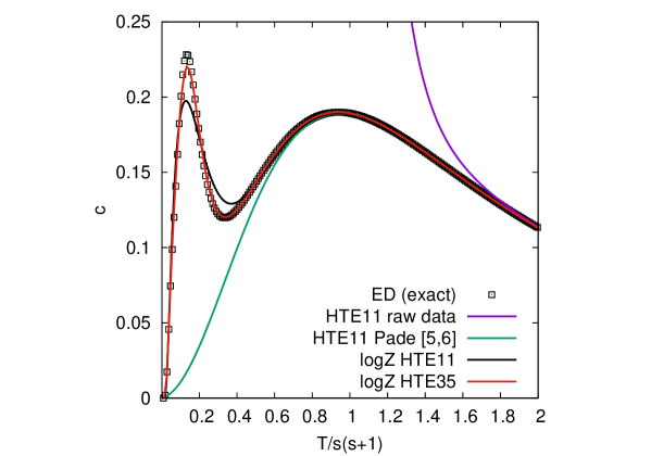
Figure 5: Specific heat $c(T)$ of the cuboctahedron for $s=1/2$, calculated by the Log Z method compared to the exact function (ED, open squares). The black solid line shows the result using one excitation and an HTE of order $n=11$, the red solid line shows analogously data for the $4$ lowest excitations and $n=35$. For comparison we also show the ‘raw’ HTE of order $n=11$ (blue curve) as well as the [5,6] Padé approximant (green curve).

To be more specific, we illustrate the Log Z method using the values and the degeneracies of the first $k$ eigenvalues of the Hamiltonian as well as the HTE of the specific heat of order $n=11$, i.e. we can use 12 HTE coefficients of $\ell(\beta)$ as input for the interpolation, cf. section III.3. This use of HTE data of order $n=11$ is based on unpublished results that exceed the published ones HTE_wir ,url_HTE10 by one order.

We write

$$\ell_{\mbox{\scriptsize int}}(\beta) = \sum_{i=1}^{k}d_{i}\,\exp(-\beta\,\delta_{i})\,\frac{\sum_{n=0}^{6}a_{n}\beta^{n}}{1+\sum_{n=1}^{5}a_{n+6}\beta^{n}\,+a_{6}\beta^{6}}$$ (33)

$$-\beta\;e_{0}\;.$$

The Padé coefficients $a_{0},\ldots,a_{11}$ are chosen such that $\ell_{\mbox{\scriptsize int}}(\beta)$ has the same first $12$ Taylor coefficients as $\log Z(\beta)$. The interpolated specific heat $c_{\mbox{\scriptsize int}}(\beta)$ is then determined according to (22). It may happen that the ansatz (33) exhibits poles in the physical temperature domain. Then one can modify the largest exponents (i.e. $n=6$ in the enumerator and $n=5$ in the denominator) to find an appropriate ansatz without poles.

In what follows we will present the temperature dependence of the specific heat using a renormalized temperature $T/s(s+1)$. This choice of the temperature scale enables the direct comparability of the $c(T)$ profiles for different values of $s$ (cf. Ref. HTE_wir, ). First we consider $s=1/2$ and compare two interpolation results for the specific heat with the exact result and also with ‘raw’ HTE data and the [5,6] Padé approximant of the HTE series. From the known complete set of eigenvalues we are also able to derive the HTE series of the specific heat up to arbitrary orders (i.e. without using the HTE code of Ref. HTE_wir, ). The results are presented in Fig. 5. If we only use the “minimal" LTA data consisting of the ground state energy and the first excitation (i.e. $k=1$ in Eq. (33)) and an HTE series up to order $n=11$ we obtain a specific heat curve that qualitatively reproduces the two maxima, but gives a height of the first maximum that is $14\%$ too low, see Fig. 5. Moreover, the position of the first maximum is slightly below the exact position. As expected, this result is significantly better than the best Padé approximant, that only reproduces the broad maximum at higher temperature.

On the other hand one may ask which “maximal data" for the LTA and HTE would give an optimal interpolation result. This is not trivial since a very large order $n$ would produce badly conditioned matrices in the calculation of the Padé coefficients. We found an optimum by considering an HTE order of $n=35$ and taking into account the first $4$ excitations $\delta_{i}$ together with their degeneracies. Since $\delta_{3}>2\,\delta_{1}$ and $\delta_{4}>3\,\delta_{1}$, the simple form (16) of the LTA is no longer valid and has to be replaced by a variant involving higher terms of the Taylor series of $\log(1+x)$. The result of the “optimal" interpolation then fits the exact curve very well, see the red line of Fig. 5, and has a maximal deviation of $4\%$ at the first maximum.

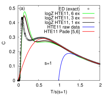
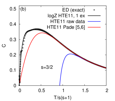
Figure 6: Specific heat $c(T)$ of the cuboctahedron for $s=1$ (a) and $s=3/2$ (b), calculated by the Log Z method compared to the exact function (ED, open squares). The black solid line shows the result using one excitation and an HTE of order $n=11$. For comparison we also show the ‘raw’ HTE of order $n=11$ (blue) as well as the [5,6] Padé approximant (red). For $s=1$ we also show results using three (brown curve) and six excitations (green) and an HTE of order $n=11$.

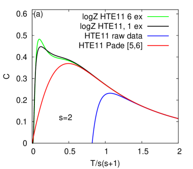
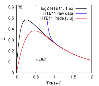
Figure 7: Specific heat $c(T)$ of the cuboctahedron for $s=2$ (a) and $s=5/2$ (b), calculated by the Log Z method. The black solid line shows the result using one excitation and an HTE of order $n=11$. For comparison we also show the ‘raw’ HTE of order $n=11$ (blue) as well as the [5,6] Padé approximant (red). For $s=2$ we also show the log Z interpolation using six excitations and an HTE of order $n=11$ (green).

In Fig. 6 we present the results of the log Z interpolation results and an HTE of order $n=11$ for spin quantum numbers $s=1$ and $s=3/2$. Again we compare with the exact results and also with ‘raw’ HTE data and the [5,6] Padé approximant of the HTE series. The specific heat for $s=1$ also exhibits an extra low-temperature maximum (located at $T/s(s+1)=0.101$) below the ordinary broad maximum, see Fig. 6a. However, both maxima are not separated by a pronounced minimum in $C(T)$ as it was found for $s=1/2$ (see Fig. 5). Rather they are smoothly connected. The important finding is that again the interpolation reproduces the extra maximum. Obviously, the quantitative agreement is less good compared to the $s=1/2$ case. Taking into account more than one excitation does not lead to an improvement of the interpolation. We conjecture that this is a hint to a general “principle of balance" saying that for a successful interpolation the input of the HTE and the LTA should be balanced. In practice, one will try to use the maximal number of HTE orders available, as long as no poles appear in the interpolated functions. It could be misleading to also use as much excitations and degeneracies as possible that are, for example, obtainable by Lanczos exact diagonalization. This need not enhance the quality of the interpolation, but may even degrade it. Using more excitations would only improve the interpolation if simultaneously higher orders of the HTE would be taken into account as, e. g., in the above case of $s=1/2$. Thus, for an HTE of order $n=11$ an LTA including, e. g., one excitation seems to be well balanced.
Moreover, we emphasize that interpolation with constraints is crucial for the correct description of $c(T)$ for intermediate temperatures: Both, the ‘raw’ HTE and the [5,6] Padé approximant do not give indications for a second maximum. It may be argued that this second maximum is produced by the necessity for the interpolated function $c_{int}(T)$ to allow for the two integral constraints (9) and (10).

The behavior of the specific heat for $s=3/2$ is somehow different, since there is no pronounced low-temperature maximum, rather $c(T)$ exhibits a broad plateau-like maximum in the region $0.13\lesssim T/s(s+1)\lesssim 0.53$ (see Fig. 6b). This feature is very well described by our interpolation scheme taking into account the first excitation, only. On the other hand, the ‘raw’ HTE and the [5,6] Padé approximant fail to yield a good description of this broad maximum. At very low temperatures a tiny extra maximum is visible in the exact data not seen in the interpolation.

Let us also emphasize that obviously the position of the broad maximum at moderate temperatures is shifted to lower values of $T/s(s+1)$ as increasing $s$. We find $T/s(s+1)=0.937$ ($s=1/2$), $T/s(s+1)=0.65$ ($s=1$) and $T/s(s+1)=0.406$ ($s=3/2$). Thus, we may speculate that the very existence of the double maximum profile of $c(T)$ is a quantum effect and will disappear as further increasing of $s$.

From the above presented comparison of exact data and results of the log Z interpolation it is evident that the minimal version, taking into account the energies of the ground state and the first excitation, leads to very good results for the specific heat in the whole temperature range. In particular, specific features such as an extra maximum in the low-temperature region can be reproduced by the interpolation scheme. Thus we may conclude, that this scheme has some predictive power that can be used for the investigation of systems, where no information on the full spectrum is available, but the energies of the ground state and the first excitation are known.

In the next step we therefore apply our approach to $s=2,5/2,3$ and $7/2$. Let us start with $s=2$ (i.e. first value of $s$ without exact data for $c(T)$) and $s=5/2$. Interestingly, for $s=2$ (Fig. 7a) a low-temperature maximum is found at $T/s(s+1)=0.12$, but there is only a remnant of the ordinary broad maximum in form of a plateau-like shoulder around $T/s(s+1)\sim 0.4$. Thus the general shape is closer to that for $s=1/2$ and $s=1$ than that for $s=3/2$.

We may interpreted this observation as another indication of the qualitative difference between half-integer and integer $s$ stemming from the fact that the three spins on a triangle can be composed to a zero total spin for integer $s$, whereas for half-integer $s$ the composed spin on a triangle is non-zero schmidt2005 . This difference is also manifested in the ground state spin-spin correlation of the cuboctahedron schmidt2005 . This observation fits also to the case $s=5/2$ shown in Fig. 7b, where $c(T)$ exhibits only one maximum without a shoulder. Concerning the low-energy spectrum, relevant for the low-temperature behavior of $c(T)$, we found for the excitation gap $\Delta=0.1165,0.6705,0.0434,0.6234,0.1006,0.5237$, and $0.12823$ for $s=1/2,1,3/2,2,5/2,3$ and $7/2$, respectively, i.e. the gap is significantly smaller for half-integer $s$ than for integer $s$.

Let us summarize our findings for the spin-$s$ Heisenberg model on the cuboctahedron. For that we collect our log Z interpolation data for all accessible values of $s$ in Fig. 8a. For comparison we also show the [5,6] Padé approximants in Fig. 8b. Obviously, for $T/s(s+1)\gtrsim 1.8$ all curves coincide, i.e. in the renormalized temperature scale the high-temperature behavior is independent of $s$ HTE_wir . For $T/s(s+1)\lesssim 1$ there is a strong influence of the spin $s$, where for low spin values $s$ some prominent extra features (shoulder, additional maximum) emerge. For larger spin $s\geq 5/2$ no significant extra features appear, rather there is one pronounced maximum. The Padé approximants describe the behavior of $c(T)$ reasonably well down to about $T/s(s+1)\sim 0.6$, i.e. the extra features at low $T$ are not covered by the Padé approximants. The height $c_{\rm max}$ and the position $T_{\rm max}/s(s+1)$ of the maxima in $c(T)$ strongly depend on $s$. As an overall tendency we observe that $c_{\rm max}$ increases and $T_{\rm max}/s(s+1)$ decreases with growing $s$, however, there is not a simple monotonic dependence on $s$ (compare $T_{\rm max}/s(s+1)$ for $s=5/2,3$ and $7/2$ in Fig. 8a).

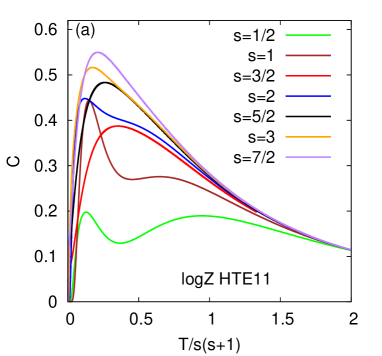
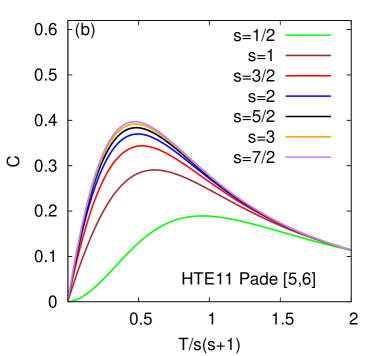
Figure 8: Specific heat $c(T)$ of the cuboctahedron for various values of the spin quantum number $s$: Comparison of the Log Z interpolation (a) with the [5,6] Padé approximants of the HTE series of order $n=11$ without interpolation (b).

V Interpolation for classical spin systems

In the classical limit $s\rightarrow\infty$ the foundations of interpolation described in section III have to be slightly reformulated. This is already clear from the divergence of the r. h. s. of the entropy integral (10). We will confine ourselves to the Log Z method.

Since the partition function $Z(\beta)$ diverges in the classical limit it has to be replaced by the normalized partition function

$$\tilde{Z}(\beta)=\frac{\mbox{Tr }e^{-\beta H}}{\mbox{Tr }{\mathbbm{1}}}=(2s+1)^{-N}\mbox{Tr }e^{-\beta H}\;.$$ (34)

The classical limit of (34) reads

$$Z^{\scriptsize\mbox{cl}}(\beta)=(4\pi)^{-N}\int_{X}e^{-\beta H(x)}\,dx\;,$$ (35)

where $X=\left({\mathcal{S}}^{2}\right)^{N}$ denotes the classical phase space of a system of $N$ spins and $dx=d\Omega_{1}\ldots d\Omega_{N}$ its volume form. Consequently, the HTE of $Z^{\scriptsize\mbox{cl}}(\beta)$ assumes the form

$$Z^{\scriptsize\mbox{cl}}(\beta)=\sum_{n=0}^{\infty}\frac{m_{n}}{n!}(-\beta)^{n}=1+\frac{m_{2}}{2}\beta^{2}+\ldots\;,$$ (36)

where $m_{n}$ denotes the $n$ th normalized moment of $H$

$$m_{n}=(4\pi)^{-N}\int_{X}H^{n}(x)\,dx\;,$$ (37)

and $m_{1}=0$ has been used. From this one can derive the HTE of other thermodynamical functions with leading terms

$$\ell(\beta) \equiv \log Z^{\scriptsize\mbox{cl}}(\beta)=\frac{m_{2}}{2}\beta^{2}+\ldots\quad,$$ (38)

$$c(\beta) = \beta^{2}\frac{\partial^{2}}{\partial\beta^{2}}\ell(\beta)=m_{2}\beta^{2}+\ldots\quad,$$ (39)

$$s(\beta) = \ell(\beta)-\beta\frac{\partial}{\partial\beta}\ell(\beta)=-\frac{m_{2}}{2}\beta^{2}+\ldots\quad.$$ (40)

Regarding the low temperature asymptotic (LTA) of the classical partition function we assume the following

$$Z^{\scriptsize\mbox{cl}}(\beta)\sim e^{-\beta e_{0}}\,\beta^{-a}\,b\quad\mbox{for }\beta\rightarrow\infty\;.$$ (41)

Here $e_{0}$ denotes the ground state energy and $a>0,\,b$ are certain parameters. (41) is, at least, satisfied for certain finite classical spin system that we have investigated, see below. Since the purpose of our paper is to demonstrate the applicability of certain concepts of interpolation and not to give a complete survey, we will confine ourselves to the above case (41). It implies the LTA

$$\ell(\beta) \sim -\beta e_{0}-a\log\beta+\ell_{0},$$ (42)

$$c(\beta) \sim a,$$ (43)

$$s(\beta) \sim a+\ell_{0}-a\log\beta\;,$$ (44)

where $\ell_{0}\equiv\log b$. Hence $a$ can be identified with the finite limit of the specific heat for zero temperature. (44) implies that $s(T)$ diverges for $T\rightarrow 0$ and hence the integral constraint (10) has to be reformulated for classical spin systems. We write

$$\Delta s \equiv s\left(\infty\right)-s\left(\frac{1}{\beta}\right)=\int_{\frac{1}{\beta}}^{\infty}\frac{ds}{dT}dT=\int_{\frac{1}{\beta}}^{\infty}\frac{c}{T}dT$$ (45)

$$= \left[c(T)\log T\right]_{\frac{1}{\beta}}^{\infty}-\int_{\frac{1}{\beta}}^{\infty}\frac{dc}{dT}\log T\,dT\;,$$ (46)

where (46) is obtained by partial integration. Since $c(T)\log T\sim m_{2}T^{-2}\log T\rightarrow 0$ for $T\rightarrow\infty$, the first term in (46) assumes the form $-c(\beta)\log\frac{1}{\beta}\sim a\log\beta$ for $\beta\rightarrow\infty$. On the other hand, $s\left(\infty\right)-s\left(\frac{1}{\beta}\right)\sim 0-a-\ell_{0}+a\log\beta$ for $\beta\rightarrow\infty$ and thus

$$\int_{\frac{1}{\beta}}^{\infty}\frac{dc}{dT}\log T\,dT\sim a+\ell_{0}\quad\mbox{for }\beta\rightarrow\infty\;.$$ (47)

The limit $\beta\rightarrow\infty$ of (47) yields the modified integral constraint

$$\int_{0}^{\infty}\frac{dc}{dT}\log T\,dT=a+\ell_{0}=a+\log\,b\;,$$ (48)

that holds for classical spin systems satisfying (41). Further partial integrations yield an infinite number of integral constraints involving higher derivatives of $c(T)$ that are, however, equivalent to (48). In the following subsections we will test the considerations of this section and the Log Z interpolation for an example that can be analytically solved.

V.1 The equilateral triangle

The partition function of the equilateral spin triangle with Hamiltonian

$$H={\mathbf{s}}_{1}\cdot{\mathbf{s}}_{2}+{\mathbf{s}}_{2}\cdot{\mathbf{s}}_{3}+{\mathbf{s}}_{3}\cdot{\mathbf{s}}_{1}$$ (49)

can be calculated analytically. The result for $Z^{\scriptsize\mbox{cl}}(\beta,B)$ given in Eq. (14) of CLAL99 , where $B$ denotes the external magnetic field, can be evaluated in the limit $B\rightarrow 0$ and yields

$$Z^{\scriptsize\mbox{cl}}(\beta)=\frac{\sqrt{\frac{\pi}{2}}e^{3\beta/2}\left(-3\,\text{erfc}\left(\sqrt{\frac{\beta}{2}}\right)+\text{erfc}\left(3\,\sqrt{\frac{\beta}{2}}\right)+2\right)}{4\,\beta^{3/2}}\;.$$ (50)

From this the specific heat can be derived in analytical form; but the result is too complicated to be presented here. The LTA of (50) is easily seen to be of the form (41) with

$$e_{0}=-\frac{3}{2},\quad a=\frac{3}{2},\quad b=\frac{\sqrt{\pi}}{2\sqrt{2}}\;.$$ (51)

This result can also be obtained without using the analytical form (50) of the partition function, see appendix A.

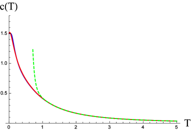
Figure 9: The specific heat $c(T)$ of the classical equilateral spin triangle. We show the analytical result (blue curve), the Log Z interpolation (red curve), and the ‘raw’ HTE of $12$th order (green dashed curve).

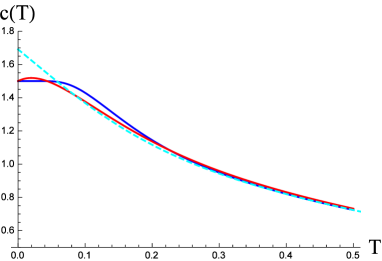
Figure 10: The same specific heat as in Fig. 9, but for lower temperatures. We show the analytical result (blue curve), the Log Z interpolation (red curve), and the HTE [6,6] Padé approximant (cyan dashed curve).

Next we consider interpolation of $c(T)$ according to the Log Z method. The LTA of $\ell(\beta)$ is not analytic at $\beta=0$, see (42). As a way out we consider the auxiliary function

$$G(\beta)=\left(Z^{\scriptsize\mbox{cl}}(\beta)\right)^{2/3}\;,$$ (52)

that has the LTA

$$G(\beta)\sim e^{\beta}\beta^{-1}\frac{\pi^{1/3}}{2}\;.$$ (53)

The factor $\beta^{-1}$ is still not analytical at $\beta=0$ but can be compensated by a suitable choice of the Padé function. It turns out that an optimal interpolation is obtained by the ansatz

$$G_{\scriptsize\mbox{int}}(\beta)=\frac{\pi^{1/3}e^{\beta}\left(a_{4}\beta^{4}+a_{3}\beta^{3}+a_{2}\beta^{2}+\frac{2\beta}{\pi^{1/3}}\right)}{2\beta\left(a_{4}\beta^{4}+a_{7}\beta^{3}+a_{6}\beta^{2}+a_{5}\beta+1\right)}\;.$$ (54)

The Padé coefficients $a_{2},\ldots,a_{7}$ are, as usual, determined by the condition that $G_{\scriptsize\mbox{int}}(\beta)$ has the same first six HTE coefficients as $\left(Z^{\scriptsize\mbox{cl}}(\beta)\right)^{2/3}$. The latter can be calculated from the analytical form of $Z^{\scriptsize\mbox{cl}}(\beta)$, but also independently by using the $C^{++}$ program provided at url_HTE10 . At the end, the interpolation of $G(\beta)$ thus obtained has to be transformed into interpolations of $Z^{\scriptsize\mbox{cl}}(\beta)$ and $c(T)$. We compare this result with the analytical form of the specific heat and with approximations based solely on HTE data of $12$-th order, see the Figs. 9 and 10. One observes that in this case the HTE [6,6] Padé approximant of $c(T)$ assumes the finite value of $c(0)=1.69087\ldots$ that is, however, $13\%$ above the correct value $c(0)=\frac{3}{2}$. We have also checked the integral constraints (9) and (48) for the analytical and the interpolation form for the specific heat by numerical integrations. The close coincidence between analytical and interpolation results shows the consistency of the present method.

VI Summary

In our paper we present an approach to evaluate the specific heat $c(T)$ of magnetic systems using an interpolation scheme between the known low-temperature and high-temperature properties of $c(T)$ that also exploits sum rules constraining the specific heat. To satisfy these sum rules for $c(T)$ it is more convenient to perform the interpolation for the logarithm of the partition function $Z$ (i.e. the free energy $F/T$). The requested input at high temperatures in form of a high-temperature expansion series of log $Z$ can be obtained by a simple C++-program HTE_wir ; url_HTE10 . The input at low temperatures in form of the ground-state energy and the behavior of $c(T)$ as $T\to 0$ can be provided by the toolbox of many-body methods designed for the low-energy degrees of freedom. As a result, the proposed interpolation scheme represents a quite universal and powerful instrument to study the specific heat, e.g., for frustrated quantum magnets and to provide model data to compare with experimental results. We demonstrate the accuracy of our approach by comparing the approximate interpolation data with exact numerical date for a nontrivial strongly frustrated model system, the spin-$s$ Heisenberg antiferromagnet on the cuboctahedron. In particular, we found evidence that a prominent feature in form of an additional low-temperature maximum in $c(T)$ can be detected by the interpolation approximation. We may conclude that the log Z interpolation scheme has some predictive power that can be used for the investigations of strongly frustrated quantum spin systems, where other tools, such as the quantum Monte Carlo technique, are not applicable.

Appendix A LTA of the classical spin triangle

We will show how to obtain the result (51) that is needed for the interpolation of the specific heat without using the analytical form of $Z^{\scriptsize\mbox{cl}}(\beta)$. In fact, the LTA of $Z^{\scriptsize\mbox{cl}}(\beta)$ can be determined by the $3$-dimensional Laplace method, see F11 . First, it is clear that the lowest energy of (49) is realized by any coplanar state of three unit vectors forming mutual angles of $\frac{2\pi}{3}$ and only by such states. Hence the lowest energy is $e_{0}=-\frac{3}{2}$ and the usual rotational degeneracy of the ground state is the only one. This can be further supported by calculating the eigenvalues of the Hessian of (49). When doing this one has to be careful in choosing the right coordinates. We fix the vector

$${\mathbf{s}}_{1}=\left(\begin{array}[]{c}0\\ 0\\ 1\end{array}\right)\;,$$ (55)

and write

$${\mathbf{s}}_{2} = \left(\begin{array}[]{c}\sqrt{1-(-1/2+z_{2})^{2}}\\ 0\\ -1/2+z_{2}\end{array}\right)\;,$$ (59)

$${\mathbf{s}}_{3} = \left(\begin{array}[]{c}\sqrt{1-(-1/2+z_{3})^{2}}\cos(\pi+\varphi_{3})\\ \sqrt{1-(-1/2+z_{3})^{2}}\sin(\pi+\varphi_{3})\\ -1/2+z_{3}\end{array}\right)\;,$$ (63)

thereby utilizing full rotational symmetry. Thus the reduced phase space (the full phase space reduced by the rotational group) is described by three canonical coordinates ${\mathbf{u}}=(u_{1},u_{2},u_{3})\equiv(z_{2},z_{3},\varphi_{3})$ and the ground state corresponds to ${\mathbf{u}}={\mathbf{0}}$. We consider the matrix $H_{2}$ that is, up to a factor $1/2$, the Hessian of (49), i. e. the symmetric $3\times 3$-matrix formed by all second derivatives of the Hamiltonian $H$ w. r. t. the $u_{i},u_{j}$, evaluated at the ground state such that

$$H=e_{0}+{\mathbf{u}}\cdot H_{2}\cdot{\mathbf{u}}+{\mathcal{O}}(|{\mathbf{u}}|^{3})\;.$$ (64)

The three eigenvalues of $H_{2}$ are $h_{1}=1,\;h_{2}=\frac{3}{8},\;h_{3}=\frac{1}{3}$. They are positive in accordance with the fact that (64) is the expansion of $H$ at the ground state. Let ${\mathbf{v}}=(v_{1},v_{2},v_{3})$ denote the coordinates corresponding to the eigenbasis of $H_{2}$ that are obtained by a suitable rotation of ${\mathbf{u}}$. For low temperatures the system will stay close to the ground state and its energy $H$ can be well approximated by the second order Taylor series (64). For the integrand $e^{-\beta H}$ occurring in the integral defining the partition function we may perform the approximation

$$e^{-\beta H}\approx e^{-\beta(e_{0}+{\mathbf{u}}\cdot H_{2}\cdot{\mathbf{u}})}=e^{-\beta\left(e_{0}+\sum_{i=1}^{3}h_{i}v_{i}^{2}\right)}\;.$$ (65)

The integral of (65) over the reduced phase space can hence be approximated, besides the constant factor $e^{-\beta e_{0}}$, by the product of three Gaussian integrals of the form

$$\int_{-\infty}^{\infty}\exp\left(-\beta h_{i}\,v_{i}^{2}\right)\,dv_{i}=\sqrt{\frac{\pi}{\beta h_{i}}},\;i=1,2,3\;.$$ (66)

The product of the three integrals (66) gives $\frac{\pi^{3/2}}{\beta^{3/2}\sqrt{h_{1}h_{2}h_{3}}}=\frac{\pi^{3/2}\sqrt{8}}{\beta^{3/2}}$ and has further to be divided by $8\pi$ due to normalization. Note that the missing factor $8\pi^{2}$ is the volume of the rotational group that has to be left out since we integrate only over the reduced phase space. This gives the correct term $\beta^{-3/2}$, i. e. , $a=\frac{3}{2}$ in (41), and, further, the factor $b=\frac{\pi^{3/2}\sqrt{8}}{8\pi}=\sqrt{\frac{\pi}{8}}$ in accordance with (51), which completes the calculation of the LTA of the equilateral triangle without using the analytical result (50).

Acknowlegedments

We thank Jürgen Schnack for providing the exact data for the specific heat of the cuboctahedron with $s=3/2$. Moreover, we are grateful to Gregoire Misguich for committing to us the unpublished HTE coefficients up to order $n=20$ of the $s=1$ Haldane chain that were originally computed by Elstner, Jolicoeur, and Golinelli.

References

- (1) Quantum Magnetism, edited by U. Schollwöck, J. Richter, D. J. J. Farnell, and R. F. Bishop Lecture Notes in Physics 645, (Springer, Berlin, 2004), Introduction to Frustrated Magnetism: Materials, Experiments, Theory, edited by C. Lacroix, P. Mendels, and F. Mila, Springer Series in Solid-State Sciences, (Springer, Berlin, 2011).
- (2) Introduction to Frustrated Magnetism: Materials, Experiments, Theory, edited by C. Lacroix, P. Mendels, and F. Mila, Springer Series in Solid-State Sciences, (Springer, Berlin, 2011).
- (3) M. Troyer and U.J. Wiese, Phys. Rev. Lett. 94, 170201 (2005).
- (4) U. Schollwöck, Rev. Mod. Phys. 77, 259 (2005).
- (5) R. F. Bishop, in Microscopic Quantum Many-Body Theories and Their Applications, edited by J. Navarro and A. Polls, Lecture Notes in Physics 510 (Springer, Berlin, 1998), p.1.
- (6) O. Götze, D.J.J. Farnell, R.F. Bishop, P.H.Y. Li, and J. Richter, Phys. Rev. B 84, 224428 (2011), P. H. Y. Li, R. F. Bishop, and C. E. Campbell, Phys. Rev. B 88, 144423 (2013), O. Götze and J. Richter, Phys. Rev. B 91, 104402 (2015).
- (7) W. Metzner, M. Salmhofer, C. Honerkamp, V. Meden, and K. Schönhammer, Rev. Mod. Phys. 84, 299 (2012).
- (8) J. Reuther and P. Wölfle, Phys. Rev. B 81, 144410 (2010); J. Reuther, P. Wölfle, R. Darradi, W. Brenig, M. Arlego, and J. Richter, Phys. Rev. B 83, 064416 (2011).
- (9) J. Richter, J. Schulenburg, A. Honecker, and D. Schmalfuß, Phys. Rev. B 70, 174454 (2004).
- (10) J. Richter and J. Schulenburg, Eur. Phys. J. B 73, 117 (2010).
- (11) A. M. Läuchli, J. Sudan, and E. S. Sørensen, Phys. Rev. B 83, 212401 (2011).
- (12) S. Yan, D. A. Huse, and S. R. White, Science 332, 1173 (2011).
- (13) S. Depenbrock, I. P. McCulloch, and U. Schollwöck, Phys. Rev. Lett. 109, 067201 (2012).
- (14) Z. Y. Xie, J. Chen, J. F. Yu, X. Kong, B. Normand, and T. Xiang, Phys. Rev. X 4, 011025 (2014); H. J. Liao, Z. Y. Xie, J. Chen, Z. Y. Liu, H. D. Xie, R. Z. Huang, B. Normand, T. Xiang, arXiv:1610.04727.
- (15) G.S. Rushbrooke, G.A. Baker, and P.J. Wood, in Phase Transitions and Critical Phenomena, Vol. 3, p. 245; eds. C. Domb and M.S. Green, Academic Press, London, 1974.
- (16) J. Oitmaa, C.J. Hamer, and W.H. Zheng, Series Expansion Methods, Cambridge University Press 2006.
- (17) W. Opechowski, Physica 4, 181 (1937).
- (18) G.S. Rushbrooke and P.J. Wood, Proc. Phys. Soc. A 68, 1161 (1955).
- (19) G.S. Rushbrooke and P.J. Wood, Molecular Physics 1, 257 (1958).
- (20) P.J. Wood and N.W. Dalton, Phys. Rev. 159 , 384 (1967).
- (21) N.W. Dalton and D.E. Rimmer, Phys. Lett. 29A, 611 (1969).
- (22) N. Elstner, R.R.P. Singh, and A.P. Young, Phys. Rev. Lett. 71, 1629 (1993).
- (23) N. Elstner and A. P. Young, Phys. Rev. B 50, 6871 (1994).
- (24) R. P. P. Singh and J. Oitmaa, Phys. Rev. B 85, 104406 (2012).
- (25) H. Rosner, R.P.P. Singh, W.H. Zheng, J. Oitmaa, and W-E. Pickett, Phys. Rev. B 67, 014416 (2003).
- (26) B. Bernu, C. Lhuillier, E. Kermarrec, F. Bert, P. Mendels, R. H. Colman, and A. S. Wills , Phys. Rev. B 87, 155107 (2013).
- (27) D. E. Freedman, R. Chisnell, T. M. McQueen, Y. S. Lee, C. Payen and D. G. Nocera. Chem. Commun. 48, 64 (2012).
- (28) S.-H. Lee, C. Broholm, M. F. Collins, L. Heller, A. P. Ramirez, Ch. Kloc, E. Bucher, R. W. Erwin, N. Lacevic, Phys. Rev. B 56, 8091 (1997).
- (29) H.-J. Schmidt, J. Schnack, and M. Luban, Phys. Rev. B 64, 224415 (2001).
- (30) H.-J. Schmidt, A. Lohmann, and J. Richter, Phys. Rev. B 84, 104443 (2011); A. Lohmann, H.-J. Schmidt, and J. Richter, Phys. Rev. B 89, 014415 (2014).
-
(31)
see
http://www.uni-magdeburg.de/jschulen/HTE/ - (32) G.A. Baker, Phys. Rev. 124, 768 (1961).
- (33) B. Bernu and G. Misguich, Phys. Rev. B 63, 134409 (2001).
- (34) G. Misguich and B. Bernu Phys. Rev. B 71, 014417 (2005).
- (35) T. Jolicoeur and O. Golinelli, Phys. Rev. B 50, 9265 (1994).
- (36) S.R. White and D.A. Huse, Phys. Rev. B 48, 3844 (1993).
- (37) T. Xiang, Phys. Rev. B 58, 9142 (1998).
- (38) J. Richter, R. Schmidt, and J. Schnack, J. Magn. Magn. Mat. 295, 164 (2005).
- (39) J. Schnack, R. Schmidt, and J. Richter, Phys. Rev. B 76, 054413 (2007).
- (40) J. Schnack and R. Schnalle, Polyhedron 28, 1620 (2009).
- (41) A. Honecker and M. E. Zhitomirsky, J. Phys.: Conf. Ser. 145, 012082 (2009).
- (42) J. Schnack, Dalton Trans. 39, 4677 (2010).
- (43) A. Hucht, S. Sahoo, S. Sil, and P. Entel, Phys. Rev. B 84, 104438 (2011).
- (44) K. Karlova and J. Strecka, J. Low Temp. Phys (2106). doi:10.1007/s10909-016-1676-8 (2026) (arXiv:1611.04301)
- (45) A. J. Blake, R. O. Gould, C. M. Grant, P. E. Y. Milne, S. Parsons, and R. E. P. Winpenny J. Chem. Soc., Dalton Trans. 485-496 (1997).
- (46) M. A. Palacios, E. M. Pineda, S. Sanz, R. Inglis, M. B. Pitak, S. J. Coles, M. Evangelisti, H. Nojiri, C. Heesing, E. K. Brechin, J. Schnack, and R. E. P. Winpenny, ChemPhysChem 17, 55 (2016).
- (47) O. Ciftja, M. Luban, M. Auslender, and J.H. Luscombe, Phys. Rev. B 60, 10122 (1999).
-
(48)
Laplace method. M.V. Fedoryuk (originator), Encyclopedia of Mathematics.
URL:
http://www.encyclopediaofmath.org/index.php?title=Laplace_method&oldid=17741.