Black Hole Thermodynamics with Conical Defects

Abstract

Recently we have shown Appels:2016uha how to formulate a thermodynamic first law for a single (charged) accelerated black hole in AdS space by fixing the conical deficit angles present in the spacetime. Here we show how to generalise this result, formulating thermodynamics for black holes with varying conical deficits. We derive a new potential for the varying tension defects: the thermodynamic length, both for accelerating and static black holes. We discuss possible physical processes in which the tension of a string ending on a black hole might vary, and also map out the thermodynamic phase space of accelerating black holes and explore their critical phenomena.

1 Introduction

The idea that black holes can behave as thermodynamical objects, with a finite temperature and entropy has been one of the most fascinating yet perplexing breakthroughs in our understanding of these strongly gravitating objects Bekenstein:1973ur ; Bekenstein:1974ax ; Hawking:1974sw . Not only does this insight give consistency to thermodynamical systems in gravity, but it also gives a concrete arena for exploring quantum gravitational effects in a controlled fashion. Thermodynamical considerations also give us key insights into classical aspects of black holes in general relativity, a nice example being the black string instability Gregory:1993vy ; Gregory:1994bj , where the onset of a classical instability of black brane solutions in higher dimensional gravity occurs at the point where the entropy of the black brane drops below that of a black hole. More generally, it seems there is a link between thermodynamic and dynamical stability of black holes and branes Gubser:2000mm ; Reall:2001ag ; Hollands:2012sf . Perhaps most pertinent for the discussion here however, are the properties of black holes in anti de Sitter (AdS) space, where thermal equilibrium is straightforwardly defined Hawking:1982dh and physical processes correspond via a gauge/gravity duality to a strongly coupled dual thermal field theory Witten:1998zw .

Given the central importance of black hole thermodynamics in theoretical gravity, it is surprising that until recently only the thermodynamics of relatively simply systems had been explored. Although our catalog of exact black hole solutions is limited (mostly) to isolated gravitating systems, there is a class of intriguing exceptions, given by axisymmetric solutions to the Einstein equations Weyl ; Charmousis:2003wm , including axisymmetric multiple black holes IsraelKhan ; Dowker:2001dg ; Gibbons:1979nf ; Costa:2000kf ; Herdeiro:2009vd , black holes in magnetic flux tubes (including a study of thermodynamics) Gibbons:2013dna ; Booth:2015nwa ; Astorino:2016hls , and most pertinently for our discussion, the accelerating black hole. This last example has an exact solution known as the C-metric Kinnersley:1970zw ; Plebanski:1976gy , corresponding to a black hole with a conical deficit emerging from one pole, or unequal conical deficits emerging from each pole. Since it can be shown that the conical deficit can be replaced by a finite width topological defect RGMH , the physical interpretation of the geometry is that there is a cosmic string ‘pulling’ the black hole, thus accelerating it to infinity. Although this system does not represent an isolated black hole, it is nonetheless a legitimate gravitational solution that should be subject to the usual laws of black hole thermodynamics.

In Appels:2016uha , we made a preliminary step towards studying thermodynamics of accelerating black holes by considering fixed tension deficits in the context of slowly accelerating black holes in AdS space (see also Dutta:2005iy ; Astorino:2016xiy ; Astorino:2016ybm ). We discovered that the first law of thermodynamics was still valid, provided one identified the mass of the black hole appropriately normalised by the conical deficit. The fixing of tension was physically motivated by imagining that the black holes were accelerated by cosmic strings: topological defect solutions to some quantum field theory Vilenkin:1984ib whose tension is typically quantised in terms of the parameters of this underlying theory, and as such can only vary in discrete amounts (and only by having the underlying topological invariant also vary).

However, stepping back from this specific manifestation of the C-metric, we can at least pose the question of what happens if we do allow the tension to vary. Even with physical cosmic strings replacing the conical deficit, one can still imagine a possible scenario in which tension could jump as the merger of two accelerating black holes along a polar axis, initially with one conical deficit angle between the black holes, and a larger conical deficit emerging from the second black hole. Indeed, initial investigations of the interactions and capture of cosmic strings by black holes studied precisely the thermodynamics of the system of a black hole with a string AFV ; Martinez:1990sd ; Bonjour:1998rf (although in these cases, the black holes were not accelerating). Thus, allowing a cosmic string to have varying tension would appear to be a desirable feature in a full exploration of the thermodynamics of accelerating black holes.

In this paper we formulate laws of accelerating black hole thermodynamics, allowing for a varying tension. We perform our analysis in AdS in order to utilise solutions that have only one horizon, although the first law we derive will still apply to any horizon locally. To some extent, this is matter of technical convenience; we define temperature via a process of Euclideanization thus if more than one horizon is present, the Euclidean section will contain conical singularities. These Euclidean conical singularities are distinct from those of the accelerating black holes of the C-metric – they are not the result of sources, but instead should be viewed as necessary singularities arising from analytic continuation. They reflect the fact that different horizons can be at different temperatures (though can be integrated in a controlled fashion Gregory:2013hja ).

We first present thermodynamics of black holes with varying conical deficit in the absence of acceleration, partly as a warm-up exercise, but more importantly to motivate and isolate the impact of a varying tension deficit. We show that the correct first law of thermodynamics includes a “$\lambda\delta\mu$” term, where $\mu$ is the tension of the deficit, and $\lambda$ the corresponding thermodynamic potential. We then turn to the charged accelerating black hole and derive the general first law for accelerating black holes:

$$\delta M=T\delta S+V\delta P+\Phi\delta Q-\lambda_{+}\delta\mu_{+}-\lambda_{-}\delta\mu_{-}$$ (1)

allowing not only variation of entropy and charge, but also the cosmological constant (encoded in the thermodynamic pressure $P$ Teitelboim:1985dp ; Kastor:2009wy ; Dolan:2010ha ; Cvetic:2010jb ; Dolan:2011xt ; Kubiznak:2012wp ; Kubiznak:2016qmn ) and allowing the tensions along each axis $\mu_{\pm}$ to vary independently. We derive the corresponding thermodynamic lengths for each tension, as well as the appropriate expressions for the normalised thermodynamic mass and electromagnetic potential. Analogous to the rotating AdS black hole Gibbons:2004ai , we find that the electromagnetic potential and thermodynamic mass are modified beyond the simple geometric conical deficit factor. Finally, we explore the physical consequences of our results.

2 Thermodynamics with Conical Deficits

Before discussing the accelerating black hole, it is interesting to revisit the thermodynamics of a black hole with a ‘cosmic string’: a spacetime first studied by Aryal, Ford and Vilenkin (AFV) AFV . AFV considered a conical deficit through a Schwarzschild black hole:

$$ds^{2}=f(r)dt^{2}-\frac{dr^{2}}{f(r)}-r^{2}d\theta^{2}-r^{2}\sin^{2}\theta\left(\frac{d\phi}{K}\right)^{2}$$ (2)

where $f(r)=1-2m/r$. They considered a first law of thermodynamics to argue that the entropy of the black hole remained at one quarter of its area, now containing a factor of $K$: $S=\pi r_{+}^{2}/K$. The thermodynamics of a black hole with a string was also considered in greater thoroughness by Martinez and York Martinez:1990sd , although the ‘tension’ of the cosmic string, (defined later in (5)) was held fixed. The only context in which a ‘varying’ tension was considered was in Bonjour:1998rf , where the varying tension was produced by the capture of a moving cosmic string by a black hole, and it was argued that in the collision of a black hole and cosmic string, the black hole would retain a portion of the string thus increasing its mass.

We will revisit this static system first, as a means of exploring the impact of varying tension on black hole thermodynamics. We will consider a charged black hole represented by the metric (2), with

$$f(r)=1-\frac{2m}{r}+\frac{e^{2}}{r^{2}}+\frac{r^{2}}{\ell^{2}}\;,\qquad\text{and}\quad{B}=-\frac{e}{r}dt\;.$$ (3)

The parameters $m$ and $e$ are related to the black hole’s mass, and charge respectively, $B$ is the Maxwell potential, and we allow for a negative cosmological constant via $\ell=\sqrt{-\Lambda/3}$.

In order to treat varying tension we leave the parameter $K$ in (2) unspecified. Typically, this parameter would simply be unity (or a function of rotation in the Kerr-AdS case), however, by keeping $K$ explicitly in the metric we can study conical defects through a well-behaved system in a straightforward manner.

Examining the geometry near $\theta_{+}=0$ and $\theta_{-}=\pi$ reveals how the parameter $K$ relates to the conical defect. Near the poles, the metric becomes

$$ds_{\mathrm{II}}^{2}=r^{2}\left[d\vartheta^{2}+\frac{\vartheta^{2}}{K^{2}}d\phi^{2}\right],$$ (4)

on surfaces of constant $t$ and $r$, where $\vartheta=\pm(\theta-\theta_{\pm})$ is the ‘distance’ to either pole. If $K\neq 1$, there will be a conical defect along the axis of revolution, which corresponds to a cosmic string of tension

$$\mu=\frac{\delta}{8\pi}=\frac{1}{4}\bigg{[}1-\frac{1}{K}\bigg{]},$$ (5)

where $\delta$ is the conical deficit. The interpretation of tension is justified by analysing the equations of motion for an actual cosmic string vortex in the presence of a black hole AGK , where (2) was obtained as the asymptotic form of the metric outside the string core. A tensionless string corresponds to a regular pole, $K=1$, and in this metric, the tension along either polar axis is equal, allowing simultaneous regularisation of the two poles. The static black hole is inertial, as the deficits balance each other out. This exercise provides insight into the role $K$ plays within a metric. Different values for this parameter determine the severity of an overall defect running through the black hole.

Now let us consider the temperature and entropy of the black hole. We compute $T$ by demanding regularity of the Euclidean section of the black hole Gibbons:1976ue , giving

$$T=\frac{f^{\prime}(r_{+})}{4\pi}=\frac{1}{2\pi r_{+}^{2}}\left[m-\frac{e^{2}}{r_{+}}+\frac{r_{+}^{3}}{\ell^{2}}\right]$$ (6)

thus

$$2TS=\frac{m}{K}-\frac{e}{r_{+}}\left(\frac{e}{K}\right)+2\left(\frac{3}{8\pi\ell^{2}}\right)\left(\frac{4\pi}{3K}r_{+}^{3}\right)=M-\Phi_{H}Q+2PV$$ (7)

gives a Smarr formula Smarr:1972kt for the black hole, where $M=m/K$ is the mass of the black hole, $Q=\frac{1}{4\pi}\int\star dB=e/K$ is the charge on the black hole, $\Phi_{H}=e/r_{+}$ the potential at the horizon, and $P=3/8\pi\ell^{2}$, $V=4\pi r_{+}^{3}/3K$ the thermodynamic pressure and volume respectively Teitelboim:1985dp ; Kastor:2009wy ; Dolan:2010ha ; Cvetic:2010jb ; Dolan:2011xt ; Kubiznak:2012wp ; Kubiznak:2016qmn .

Now let us consider the effect of changing the parameters of the black hole a small amount; the location of the horizon of the black hole will also shift so that $(f+\delta f)=0$ at $(r_{+}+\delta r_{+})$:

$$0=f^{\prime}(r_{+})\delta r_{+}-\frac{2\delta m}{r_{+}}+\frac{2e\delta e}{r_{+}^{2}}-2r_{+}^{2}\frac{\delta\ell}{\ell^{3}}$$ (8)

However, we can now replace the variation of the parameters $m,e,\ell$ with the variation of the corresponding thermodynamic charges $M,Q,P$, and the variation of $r_{+}$ with that of entropy, with the important proviso that we must allow for the variation of tension through $K$. Thus $\delta m=K\delta M+M\delta K$ etc. and $\delta K=4K^{2}\delta\mu$ from (5). After some rearrangement, (8) gives our first law of Thermodynamics with varying tension:

$$\delta M=T\delta S+V\delta P+\Phi_{H}\delta Q-2\lambda\delta\mu$$ (9)

where

$$\lambda=\left(r_{+}-KM\right)$$ (10)

is a thermodynamic length conjugate to the string tension. This is the central result of our paper – that string tension (in this case equal along each axis) can be thought of as analogous to a thermodynamic charge that therefore has a corresponding thermodynamic potential. Rather than write a single “$\lambda\delta\mu$” term, instead we write two “$\lambda\delta\mu$” terms, referring to the deficits emerging from each pole. Although these are obviously equal in this case, for accelerating black holes the string tensions from each pole are not the same, and we therefore separate these out now.

Surprisingly perhaps, this thermodynamic length is not simply the geometric length $r_{+}$ of the string from pole to singularity. Instead, the mass-dependent adjustment emphasises this is a potential, rather than just an internal energy term that might more appropriately be placed on the left hand side of the equation.

To see why this is the case, consider the first law in action: the capture, and subsequent escape, of a cosmic string by a black hole. This example was first proposed in Bonjour:1998rf in the case of a charged vacuum black hole. The idea is that the string is moving and gets briefly captured by the black hole. In the capture process, the internal energy of the black hole should remain fixed: the physical intuition is that if a cosmic string were to pass through a spherical shell of matter, energy conservation would demand that the spherical shell still have the same total energy throughout the process, thus either it would become denser, or its radius would increase. Of course, in the case of the spherical shell, the cosmic string would simply transit through, leaving the system. For the black hole however, we will see this is not the case, and we have the interpretation of a segment of string having been captured by the black hole, with the black hole increasing its mass accordingly. (This process was considered in the probe limit in Lonsdale:1988xd ; DeVilliers:1997nk .) We therefore consider the vacuum Reissner-Nordstrom (RN)

$$f(r)=1-\frac{2m}{r}+\frac{e^{2}}{r^{2}}$$ (11)

with the charge of the black hole being defined via $Q=e/K$, and the electric potential being $\Phi=e/r_{+}$.

Let us suppose that the string is light, or $\mu\ll 1$, then in the first stage where the black hole captures the string, fixing $M$ and $Q$ implies $\delta m=4m\delta\mu$ and $\delta e=4e\delta\mu$ (to first order in $\mu$). Thus

$$T\delta S=\frac{r_{+}-r_{-}}{4\pi r_{+}^{2}}\left[2\pi r_{+}\delta r_{+}-4\pi r_{+}^{2}\delta\mu\right]=(r_{+}-r_{-})\delta\mu=2\lambda\delta\mu$$ (12)

as required. Interestingly, because the internal energy has been fixed, the event horizon has to move outwards to compensate for the conical deficit. Since the entropy contains just one factor of $K$, but two of $r_{+}$, the net effect is an increase of entropy, indicating this is an irreversible thermodynamic process. The one interesting exception being an extremal black hole.

In the second step, the string pulls off the black hole, so $\delta\mu=-\mu$, and since the string is uncharged, $\delta Q$ must remain zero, and $e$ returns to its original value. However, since entropy cannot decrease, $M$ must increase

$$\delta M=T\delta S+2(r_{+}-m)\mu=\frac{(r_{+}-r_{-})\delta r_{+}}{2r_{+}}+2(r_{+}-r_{-})\mu$$ (13)

In Bonjour:1998rf , we supposed that $m$ did not change, leading to an increase in $M$ of $4m\mu$, that we incorrectly stated was the mass of the string behind the event horizon (this is only true for the uncharged black hole). Instead, it seems more physically accurate to suppose that $r_{+}$ does not decrease, as otherwise the local geodesic congruence defining the event horizon would appear to be contracting in contradiction to the area theorem. In this case, $\delta M=2(r_{+}-r_{-})\mu$, or the length of cosmic string trapped between the inner and outer horizons. Even if one allows the local horizon radius to shrink while maintaining constant entropy, $\delta M=(r_{+}-r_{-})\mu$: half the former amount, but still an increase of mass due to the capture of a length of cosmic string.

3 Thermodynamics of the C-metric

We would now like to turn to the more general case where the deficits emerging from each pole are no longer equal. The disparity in the size of the deficit produces an overall force in the direction of the largest conical deficit, and the geometry is described by the C-metric Kinnersley:1970zw ; Plebanski:1976gy ; Dias:2002mi ; Griffiths:2005qp ; Podolsky:2002nk . Typically, C-metrics have both black hole and acceleration horizons, however, for simplicity we wish to restrict ourselves to having only the black hole horizon, in order that we have a well-defined temperature for the space-time. Such a geometry is called the slowly accelerating C-metric Podolsky:2002nk , and we first review this geometry before turning to its thermodynamics.

3.1 The Slowly Accelerating C-metric

In this subsection we briefly review the “slowly accelerating” C-metric. The general C-metric Kinnersley:1970zw ; Plebanski:1976gy ; Dias:2002mi ; Griffiths:2005qp represents either one or two accelerating black holes with unequal conical deficits extending from each pole of the black hole either to infinity or an acceleration horizon. Although the C-metric is well-known among relativists, there are features of the specific form we will be using that are worth highlighting, discussing how they depend on the parameters of the solution.

For this paper, we will neglect rotation, hence the general charged, accelerating AdS black hole is represented by the metric and gauge potential Griffiths:2005qp :

$$ds^{2} =\frac{1}{\Omega^{2}}\Biggl{\{}f(r)dt^{2}-\frac{dr^{2}}{f(r)}-r^{2}\left[\frac{d\theta^{2}}{g(\theta)}+g(\theta)\sin^{2}\theta\frac{d\phi^{2}}{K^{2}}\right]\Biggr{\}}\;,\qquad{B}=-\frac{e}{r}dt,$$ (14)

where

$$\Omega=1+Ar\cos\theta\;,$$ (15)

is the conformal factor that will determine the location of the AdS boundary (which is not at “$r=\infty$”) in terms of the $\{r,\theta\}$ coordinates, and the functions $f(r),g(\theta)$ are

$$f(r) =(1-A^{2}r^{2})\Bigl{(}1-\frac{2m}{r}+\frac{e^{2}}{r^{2}}\Bigr{)}+\frac{r^{2}}{\ell^{2}}\;,$$ (16)

$$g(\theta) =1+2mA\cos\theta+e^{2}A^{2}\cos^{2}\theta\,.$$

Note we are using the Hong-Teo Hong:2003gx style coordinates that have a direct relation to the usual Boyer-Lindquist coordinates for the Kerr metric.

This spacetime has potential conical singularities on the axes $\theta_{+}=0$ and $\theta_{-}=\pi$. As before, we associate these conical singularities to cosmic strings with tensions $\mu_{\pm}=\delta_{\pm}/8\pi$, where $\delta_{\pm}$ are the conical deficit angles at each pole, found by expanding near $\theta=\theta_{\pm}$:

$$4\mu_{\pm}=1-\frac{g(\theta_{\pm})}{K}=1-\frac{1}{K}\left(1\pm 2mA+e^{2}A^{2}\right)$$ (17)

Clearly, $\mu_{+}\leq\mu_{-}\leq 1/4$, and in order to avoid negative tension defects, we require $\mu_{+}\geq 0$. For the majority of the paper, we fix $K$ by demanding that one axis be regular ($\mu_{+}=0$), and the other to have a positive tension cosmic string, i.e.

$$K=g(\theta_{+})=1+2mA+e^{2}A^{2}\quad\Rightarrow\qquad\mu_{-}=\frac{mA}{K}$$ (18)

however in the interests of generality we will keep $\mu_{+}$ and $\mu_{-}$ as independent variables.

In order to understand the structure of this accelerating black hole, it is useful to consider the effects of the various parameters. Although we suspect $m$ and $e$ play the roles of mass and charge for the black hole, the original form of the C-metric has these variables defined slightly differently. In order to check this, consider the Komar integral for the mass using the method described in Magnon:1985sc

$$M_{K}=\frac{1}{8\pi}\int_{S^{2}}\star d\xi-\frac{1}{4\pi}\int n_{a}R^{a}_{b}\xi^{b}\sqrt{h}d^{3}x=\frac{m}{K}$$ (19)

where $\xi=\partial_{t}$ is a timelike Killing vector field, the first integral is performed over a $\{\theta,\phi\}$ surface of topology $S^{2}$ considered to be near infinity, and the second integral is performed throughout the interior of this surface at constant ‘time’ (as defined by $\xi$). Note this integral is actually independent of $A$, hence we can associate $m$ with the bare mass of the black hole, whether accelerating or not. Similarly, $e$ is related to the charge of the black hole:

$$Q=\frac{1}{4\pi}\int_{S^{2}}\star dB=\frac{e}{K}$$ (20)

We have already seen how the parameter $K$ is related to the conical deficits, thus the only remaining parameter to explore is $A$. In order to understand the structure of the spacetime and the relevance of $A$, first consider the Rindler space found by setting $m=e=0$ in (14):

$$ds^{2}=\frac{1}{\Omega^{2}}\Biggl{[}\left(1+\frac{r^{2}}{\ell^{2}}(1-A^{2}\ell^{2})\right)dt^{2}-\frac{dr^{2}}{1+\frac{r^{2}}{\ell^{2}}(1-A^{2}\ell^{2})}-r^{2}\left(d\theta^{2}+\sin^{2}\theta d\phi^{2}\right)\Biggr{]}$$ (21)

This spacetime no longer has a conical singularity and is locally pure AdS, however in these coordinates the boundary of AdS is not at $r=\infty$, but at $r=-1/(A\cos\theta)$. For $\theta$ in the southern hemisphere, this occurs at finite $r$, but in the northern hemisphere $r=\infty$ lies within the AdS spacetime (see figure 1). To transform to global AdS coordinates $\{R,\Theta\}$, one takes Podolsky:2002nk

$$1+\frac{R^{2}}{\ell^{2}}=\frac{1+(1-A^{2}\ell^{2})r^{2}/\ell^{2}}{(1-A^{2}\ell^{2})\Omega^{2}}\qquad;\qquad R\sin\Theta=\frac{r\sin\theta}{\Omega}$$ (22)

the boundary, $R\to\infty$ now clearly corresponds to $\Omega\to 0$, and the origin of Rindler coordinates corresponds to $R_{0}=A\ell^{2}/\sqrt{1-A^{2}\ell^{2}}$, i.e. the Rindler coordinates represent those of an observer displaced from the origin of AdS, clearly requiring $A\ell<1$. If $A\ell=1$, (21) simply becomes the Poincaré patch of AdS, with a horizon appearing at $z=r\cos\theta=-\ell$. The C-metric with $A\ell=1$ was considered in Emparan:1999wa .

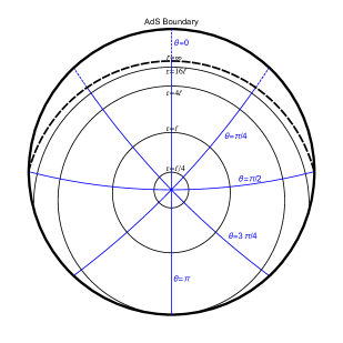
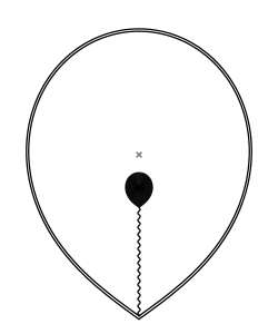
Figure 1: Left: The slowly accelerating Rindler spacetime shown here with $A\ell=1/4$, and $\ell=1$ for simplicity. The spatial sections of AdS have been compactified to a Poincaré disc, with the constant $r$ Rindler coordinate indicated in black and constant $\theta$ in blue. The origin of the Rindler coordinates is clearly visible as being displaced from the centre of the disc, with the limit of the $r-$coordinate being the thick dashed black line. Right: The black hole distorts the Poincaré disc with a conical deficit, and is displaced from the origin of AdS. The spacetime is again static, and a cross section is shown.

Adding in a black hole now introduces a conical singularity as described above, as well as a black hole horizon $f(r_{+})=0$, given by a rather unhelpful algebraic expression. If $A\ell>1$, the black hole will have an acceleration horizon at large $r$, and if $A\ell<3\sqrt{3}/4\sqrt{2}\simeq 0.919$, there is only the black hole event horizon present in the spacetime. However, as a consequence of picking the Hong-Teo coordinates and parametrisation, the boundary between having or not having an acceleration horizon no longer lies at a single value of $A\ell$ but is instead determined by a mass dependent relation. For $3\sqrt{3}/4\sqrt{2}<A\ell<1$, there can be an acceleration horizon beyond $r=\infty$ for suitable values of $mA<1/2$. Typically, in holographic applications, the conical deficit of the C-metric is desired to be cloaked by such an horizon Hubeny:2009kz , however, in our case we are interested in thermodynamics, so to keep our thermodynamic variables unambiguous, we will take $A$ sufficiently small so that we have a single horizon, that of the black hole, and thus a well-defined temperature corresponding to the periodicity of Euclidean time at the regular Euclidean black hole horizon. We refer to this as a slowly accelerating black hole, and for clarity in plots we will simply indicate this boundary as the value $A\ell=1$. A comprehensive exploration of the structure of AdS C-metric spacetimes, including their distortion of the boundary, was given in Krtous:2005ej .

3.2 Thermodynamics of the Slowly Accelerating C-metric

In this section we perform a similar analysis to that of the string threading the black hole, but now we must allow for the tension of each of the conical deficits of the C-metric to vary. We start by finding the temperature and entropy of the black hole using the conventional relations

$$T =\frac{f^{\prime}(r_{+})}{4\pi}=\frac{1}{2\pi r_{+}^{2}}\left[(1-A^{2}r_{+}^{2})\left(m-\frac{e^{2}}{r_{+}}\right)+\frac{r_{+}^{3}}{\ell^{2}(1-A^{2}r_{+}^{2})}\right]$$ (23)

$$S =\frac{\rm Area}{4}=\frac{\pi r_{+}^{2}}{K(1-A^{2}r_{+}^{2})}$$

checking the Smarr relation, we compute

$$2TS=\frac{m}{K}-\frac{e^{2}}{Kr_{+}^{2}}+\frac{r_{+}^{3}}{K\ell^{2}(1-A^{2}r_{+}^{2})^{2}}$$ (24)

The charge of the black hole is given by (20), $Q=e/K$, and defining

$$V=\frac{4\pi r_{+}^{3}}{3K(1-A^{2}r_{+}^{2})^{2}}$$ (25)

as the modified thermodynamic volume, we obtain

$$\frac{m}{K}=2TS+Q\Phi_{H}-2PV\,.$$ (26)

Although it is tempting to identify $M=m/K$, this would be to ignore the asymptotics of the spacetime. The experience of the rotating AdS black hole Gibbons:2004ai is that thermodynamic potentials should be normalised at infinity, and in the case of rotation, the Boyer-Lindquist coordinates give a boundary that is rotating. Subtracting off this rotation leads to an extra renormalisation of the thermodynamic mass, a correct Smarr formula and correct first law.

Here, however, we cannot simply perform a similar electromagnetic gauge transformation. Our electrostatic potential no longer vanishes at infinity, and our boundary has an electric flux from pole to pole

$$F=eA\sin\theta\,dt\wedge d\theta$$ (27)

We obviously cannot subtract this charge, as that would be a physical change, but it does lead us to suspect that there may be a renormalization of electrostatic potential and thermodynamic mass. We will show how to do this presently, but first consider just the uncharged black hole, and consider variations in the position of the horizon as in (8):

$$\delta f(r_{+})=f_{+}^{\prime}\delta r_{+}-2\frac{\delta m}{r_{+}}(1-A^{2}r_{+}^{2})-2A\delta Ar_{+}(r_{+}-2m)-2\frac{r_{+}^{2}}{\ell^{3}}\delta\ell=0$$ (28)

The procedure is similar to the previous section, but we now have more algebra involved in the variation of the thermodynamic parameters. For example, in relating $\delta r_{+}$ to $\delta S$, we have:

$$\delta S=\frac{2\pi r_{+}\delta r_{+}}{K(1-A^{2}r_{+}^{2})^{2}}+\frac{2\pi r_{+}^{4}A\delta A}{K(1-A^{2}r_{+}^{2})^{2}}-\frac{\pi r_{+}^{2}}{(1-A^{2}r_{+}^{2})}\frac{\delta K}{K^{2}}$$ (29)

where our expressions for the tensions (17) give

$$\frac{\delta K}{K^{2}}=2\left(\delta\mu_{+}+\delta\mu_{-}\right)\quad;\qquad\frac{m}{K}\delta A=-\left[\delta\mu_{+}-\delta\mu_{-}+A\delta(\frac{m}{K})\right]\,.$$ (30)

Defining $M=m/K$, after some algebra one gets

$$\delta M=V\delta P+T\delta S-\delta\mu_{+}\left[\frac{r_{+}}{1+Ar_{+}}-KM\right]-\delta\mu_{-}\left[\frac{r_{+}}{1-Ar_{+}}-KM\right]\,.$$ (31)

Thus, the accelerating black hole has the same thermodynamic first law as the non-accelerating black hole, but now with a thermodynamic length for the piece of string attaching at each pole:

$$\lambda_{\pm}=\frac{r_{+}}{1\pm Ar_{+}}-KM$$ (32)

This obviously agrees with (10) for the string threading the black hole, where $r_{+}$ has now been replaced by $r_{+}/\Omega(r_{+},\theta_{\pm})$ at each pole. Note, a remarkably similar expression was obtained by Kastor and Traschen Kastor:2012dt in the context of a “Kaluza-Klein-like” gravitational tension (see e.g. Traschen:2001pb ; Harmark:2004ch ) associated to the rotational symmetry of the black hole.

Now let us consider the addition of charge. Following the same procedure of varying the horizon as before leads to the relation

$$\delta(\frac{m}{K})=T\delta S+V\delta P+\Phi_{H}\delta Q-\frac{r_{+}\delta\mu_{+}}{1+Ar_{+}}-\frac{r_{+}\delta\mu_{-}}{1-Ar_{+}}+\frac{m\delta K}{2K^{2}}$$ (33)

where now our expressions for the tensions lead to

$$\frac{m}{K}\delta A =-\delta\mu_{+}+\delta\mu_{-}-A\delta\left(\frac{m}{K}\right)$$ (34)

$$[1-e^{2}A^{2}]\frac{\delta K}{2K^{2}} =A^{2}e\delta Q-\frac{e^{2}A^{2}}{m}\delta\left(\frac{m}{K}\right)+\delta\mu_{+}\left[1-\frac{Ae^{2}}{m}\right]+\delta\mu_{-}\left[1+\frac{Ae^{2}}{m}\right]$$

Keeping an open mind, we define our thermodynamic mass and electrostatic potential as:

$$M=\gamma(e,A)\frac{m}{K}\quad;\qquad\Phi=\Phi_{H}-\Phi_{0}$$ (35)

where $\Phi_{0}$ is a correction, re-zeroing the potential, analogous to the correction of the angular potential of the Kerr-AdS black hole, but without the corresponding interpretation of being the value of the original potential at infinity.

Next, we compare

$$\delta M =\gamma\delta\left(\frac{m}{K}\right)+\frac{m}{K}(\gamma_{e}\delta e+\gamma_{A}\delta A)$$ (36)

$$=\gamma\delta\left(\frac{m}{K}\right)+m\gamma_{e}\delta Q+me\gamma_{e}\frac{\delta K}{K^{2}}+\gamma_{A}\frac{m}{K}\delta A$$

to

$$T\delta S+V\delta P+\Phi\delta Q-\lambda_{+}\delta\mu_{+}-\lambda_{-}\delta\mu_{-}=\delta\left(\frac{m}{K}\right)-\Phi_{0}\delta Q-\frac{m\delta K}{2K^{2}}$$ (37)

$$+\left[\frac{r_{+}}{1+Ar_{+}}-\lambda_{+}\right]\delta\mu_{+}+\left[\frac{r_{+}}{1-Ar_{+}}-\lambda_{-}\right]\delta\mu_{-}$$

where $\lambda_{\pm}$ are to be determined. After some algebra, we obtain

$$\delta M -T\delta S-V\delta P-\Phi\delta Q+\lambda_{+}\delta\mu_{+}+\lambda_{-}\delta\mu_{-}$$ (38)

$$=\left[(1-e^{2}A^{2})\gamma-2e^{3}A^{2}\gamma_{e}-A(1-e^{2}A^{2})\gamma_{A}-1\right]\frac{\delta\left({m/K}\right)}{(1-e^{2}A^{2})}$$

$$+\left[m(1+e^{2}A^{2})\gamma_{e}+mA^{2}e+(1-e^{2}A^{2})\Phi_{0}\right]\frac{\delta Q}{(1-e^{2}A^{2})}$$

$$+\left[\lambda_{+}-\frac{r_{+}}{1+Ar_{+}}-\gamma_{A}+\frac{(2e\gamma_{e}+1)}{1-e^{2}A^{2}}\left(m-e^{2}A\right)\right]\delta\mu_{+}$$

$$+\left[\lambda_{-}-\frac{r_{+}}{1-Ar_{+}}+\gamma_{A}+\frac{(2e\gamma_{e}+1)}{1-e^{2}A^{2}}\left(m+e^{2}A\right)\right]\delta\mu_{-}$$

for our first law to hold, clearly the RHS of this equation must vanish, leading to a constraint for $\gamma$:

$$(1-e^{2}A^{2})\gamma-2e^{3}A^{2}\gamma_{e}-A(1-e^{2}A^{2})\gamma_{A}=1\quad\Rightarrow\qquad\gamma=\frac{1}{1+e^{2}A^{2}}$$ (39)

thus specifying our thermodynamic mass and determining $\Phi_{0}$ and $\lambda_{\pm}$:

$$M =\frac{m}{K(1+e^{2}A^{2})}$$ (40)

$$\Phi_{0} =\frac{meA^{2}}{1+e^{2}A^{2}}$$

$$\lambda_{\pm} =\frac{r_{+}}{1\pm Ar_{+}}-\frac{m(1-e^{2}A^{2})}{(1+e^{2}A^{2})^{2}}\mp\frac{e^{2}A}{(1+e^{2}A^{2})}$$

This is a rather unusual set of relations, the off-set of the electrostatic potential depends on mass, and the thermodynamic mass depends on charge. We view this as a consequence of the fact that for the accelerating black hole, the electric potential cannot be gauged away at infinity – there is a polar electric field at the AdS boundary, thus mass and charge are inextricably intertwined.

4 The Thermodynamic Length

To recap, we have shown that allowing for a varying conical deficit in black hole spacetimes, the first law of thermodynamics becomes

$$\delta M=T\delta S+V\delta P+\Phi\delta Q-\lambda_{+}\delta\mu_{+}-\lambda_{-}\delta\mu_{-}$$ (41)

where the relevant thermodynamical variables are given in (40). In order to accommodate varying tension, we have to define a thermodynamic length,

$$\lambda_{\pm}=\frac{r_{+}}{1\pm Ar_{+}}-\frac{m(1-e^{2}A^{2})}{(1+e^{2}A^{2})^{2}}\mp\frac{e^{2}A}{(1+e^{2}A^{2})}$$ (42)

for each conical deficit emerging from each pole. This length consists of a direct geometrical part, a mass dependent correction, and finally, a shift in the presence of charge.

It is interesting to compare this mass-dependent shift of the thermodynamic length to the correction of the thermodynamic volume for a rotating black hole Cvetic:2010jb ; Dolan:2011jm :

$$V=\frac{4\pi}{3}\left\{\frac{r_{+}(r_{+}^{2}+a^{2})}{K}+a^{2}M\right\}$$ (43)

In this case, the first term is the expected geometric volume of the interior of the black hole, the second term being a rotation dependent correction. With this appropriately shifted thermodynamic volume, the black hole always satisfies a Reverse Isoperimetric Inequality Cvetic:2010jb , that is to say, the entropy of a black hole of a given thermodynamic volume is always maximised for the purely spherical (Schwarzschild) black hole. (We verified in Appels:2016uha that the accelerating black hole satisfies the reverse isoperimetric inequality; allowing tension to vary does not alter this result.)

Notice that the correction term for this thermodynamic volume is always positive, whereas the correction term for thermodynamic length is actually negative. This means that for large enough mass, the thermodynamic length itself becomes negative, as shown in figure 2 for an uncharged black hole. The picture for a charged black hole is similar, although the critical value of $M$ for which $\lambda_{-}$ becomes negative is larger.

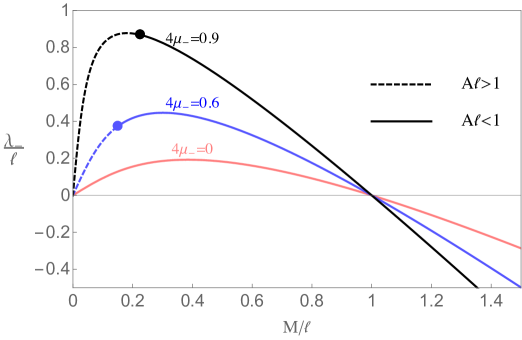
Figure 2: A plot of thermodynamic length of the south pole tension for regular north pole, $\mu_{+}=0$. The limit of the Schwarzschild-AdS black hole is shown in pink ($\mu_{-}=0$). The slowly accelerating régime, $A\ell<1$, is shown as a solid line, and $A\ell>1$ is shown dashed.

From figure 2, we see that the thermodynamic length becomes negative for ‘large’ black holes, i.e. those for which the thermodynamic mass is of similar order (or higher) than the AdS scale. Setting this in the context of the ‘cosmic string’ capture process considered in section 2 for the vacuum black hole, this would mean that the thermodynamic mass must increase during a capture, as entropy cannot decrease. This seems at first counter to the notion that the string itself does not carry ‘ADM’ mass, however, the heuristic argument of section 2 relies somewhat on the notion that a cosmic string and black hole can be sufficiently separated so that one can consider their thermodynamical (and other) properties independently. For large black holes in AdS this is manifestly not the case.

It is also interesting to compare these results for varying tension to our previous work Appels:2016uha , where $K$ and $\mu_{\pm}$ were held fixed. With these assumptions, $eA$ and $mA$ were fixed, however, we did not alter the thermodynamic mass from $m/K$, nor the electrostatic potential from $\Phi_{H}$. The two sets of results are consistent, since

$$\Phi_{0}Q=\frac{me^{2}A^{2}}{K(1+e^{2}A^{2})}=\frac{m}{K}\left[1-\frac{1}{1+e^{2}A^{2}}\right]=\frac{m}{K}-M$$ (44)

The shift in electrostatic potential multiplied by charge therefore balances the shift in thermodynamic mass in both the Smarr formula, and indeed the first law with the assumptions made in Appels:2016uha since $eA$ was required to be fixed. However, it is worth revisiting these assumptions in the light of our work here on varying tension.

First, notice that our charged C-metric has parameters: $m$, relating to the mass of the black hole, $e$ to its charge, $A$ to its acceleration, and $K$, that relates to an overall conical deficit. $K$ is the one parameter that has no immediately obvious physical interpretation, indeed seems more like a coordinate choice, thus fixing $K$ was natural. However, now armed with our better understanding of the metric and its thermodynamics, we see that in fixing the tensions of the deficits, we are fixing two physical quantities, thus we should only find that two combinations of the solution parameters are fixed. Therefore, we should not fix $K$ a priori, but instead just the combinations of parameters that fix the tensions:

$$2(\mu_{+}+\mu_{-}) =1-\frac{1+e^{2}A^{2}}{K}$$ (45)

$$\mu_{+}-\mu_{-} =-\frac{mA}{K}$$

From these expressions, we see that if charge vanishes, then indeed fixing tensions fixes $K$ and the combination $mA$, but if charge does not vanish, then we can no longer conclude that $\delta K=0$. Instead

$$\frac{\delta K}{K}=\frac{\delta(mA)}{mA}=2\frac{eA\delta(eA)}{1+e^{2}A^{2}}$$ (46)

i.e. we have two constraints on the variation of our parameters. Thus, for example if we throw a small mass $m_{0}$ into the black hole, we expect $\delta M=m_{0}$, $\delta Q=\delta P=0$. Using the expression for $M$ and the tensions we then find:

$$\frac{\delta K}{K^{2}} =-2\frac{e^{2}A^{2}}{m}\delta M \delta A =-(1-e^{2}A^{2})\frac{AK}{m}\delta M$$ (47)

$$\delta m =(1-3e^{2}A^{2})K\delta M \delta e =-2\frac{e^{3}A^{2}K}{m}\delta M$$

indicating that the acceleration of the black hole drops, as expected.

5 Critical Behaviour of Accelerating Black Holes

Given that we are working in anti-de Sitter spacetime, we can ask whether there is something analogous to a Hawking-Page phase transition Hawking:1982dh for our accelerating black holes, although it is difficult to see how one could actually have a phase transition between a system with a conical deficit along one polar axis only, and a presumably totally regular radiation bath. However, recall that a black hole in AdS behaves similarly to a black hole in a reflecting box, with the negative curvature of the AdS providing the qualitative reflection. For small black holes, the effect of the negative curvature is sub-dominant to the local curvature of the black hole, and the black hole has negative specific heat, as in the vacuum Schwarzschild case. For black holes larger than the AdS radius, the vacuum curvature dominates, and the black hole has positive specific heat, in particular, there is a minimum temperature for a black hole in AdS, below this temperature, only a radiation bath can be a solution to the Einstein equations at finite $T$. Plotting the Gibbs free energy as a function of temperature shows both the allowed states, as well as the preferred one for a given temperature. At very low $T$, the only allowed state is a radiation bath. Above a critical temperature $T_{c}=\sqrt{3}/2\pi\ell$, one can have either a radiation bath, or a black hole (that may be either ‘small’ or ‘large’). However for $T>1/\pi\ell$, the large black hole is not only thermodynamically stable (in the sense of positive specific heat) but thermodynamically preferred, and a radiation bath will spontaneously transition into a large black hole.

First consider the situation where our accelerating black hole is uncharged. Fixing the tension of the string, we can plot the temperature of our black hole as a function of its mass, $M$, as shown in figure 3. This figure shows how increasing acceleration actually makes a black hole of given mass more thermodynamically stable in the sense of positive specific heat. Figure 3 also shows the corresponding Gibbs free energy, indicating the would-be Hawking-Page transition occurs at lower temperatures as acceleration increases.

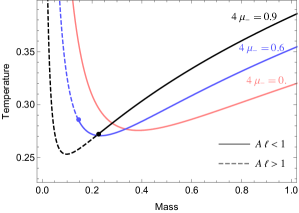
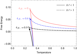
Figure 3: Left: A plot of temperature as a function of mass (in units of $\ell$) for the uncharged black hole. The slowly accelerating régime is shown as a solid line, and the inferred local horizon temperature for $A\ell>1$ is shown dashed. Note how for larger string tension (hence greater acceleration) the region of positive specific heat increases. Right: A similar plot, but now showing the Gibbs free energy as a function of temperature.

At first sight, this is rather curious, as a naive examination of the uncharged C-metric shows that the Newtonian potential, $f(r)$ has the cosmological constant ameliorated by the acceleration: $f(r)=r^{2}(1/\ell^{2}-A^{2})\simeq r^{2}/\ell_{\rm eff}^{2}$. Given that one often imagines that it is the black hole radius relative to the confining ‘box’ of AdS that is causing the thermodynamic stability of the large black holes, this looks rather confusing: increasing acceleration appears to counteract the AdS length scale. However, this intuition is too naive: the relevant effect is the spacetime curvature in the vicinity of the horizon, and whether the black hole or the cosmological constant is dominant (larger black holes having smaller tidal forces). Computing the Kretschmann scalar at the event horizon demonstrates that indeed, increasing acceleration for a given mass lowers the local tidal forces due to the black hole. In fact, it is easy to compute the “Hawking-Page” transition temperature, assuming the radiation bath to have zero Gibbs energy from the expressions for $TS$ and $M$ in terms of $r_{+}$, $A$ and $\ell$. A brief calculation gives

$$T_{HP}(r_{+},\ell,A) =\frac{1}{4\pi r_{+}}\left[\frac{3r_{+}^{2}}{\ell^{2}(1-A^{2}r_{+}^{2})}+1\right]$$ (48)

$$\simeq\frac{1}{2\pi\ell}\left(1-\frac{3}{2}A^{2}\ell^{2}+{\cal{O}}(A^{4}\ell^{4})\right)\;.$$

While the acceleration parameter $A$ is not a thermodynamic charge, instead being related to the tension via $M$, nonetheless, the general picture is that increasing tension increases acceleration, thereby decreasing the temperature at which the “Hawking-Page” transition occurs.

Now consider adding a charge to the black hole, for which we might now expect a richer phase structure, possibly with critical phenomena analogous to the isolated charged AdS black hole Chamblin:1999tk ; Cvetic:1999ne ; Chamblin:1999hg . The critical phenomena occur due to the three possible phases of black hole behaviour for varying mass. In the presence of charge, there is now a lower limit on the mass parameter of the black hole, set by the extremal limit where the temperature vanishes. Increasing the mass of the black hole moves it away from extremality, thus increasing temperature, rendering the specific heat positive near this lower limit. For large mass black holes, we are also in a positive specific heat régime where the local vacuum curvature is dominant in the near horizon geometry. Depending on the size of the charge relative to the vacuum energy, there can be an additional negative specific heat régime where the black hole is small enough that its local curvature is dominant, but is far enough from extremality that the usual Schwarzschild negative specific heat type of behaviour pervades. Given that for uncharged accelerating black holes, increasing tension lowers the critical temperature at which the transition to positive specific heat occurs, we expect this ‘swallowtail’ behaviour to be mitigated for charged accelerating black holes in the canonical ensemble, and indeed this is what is observed.

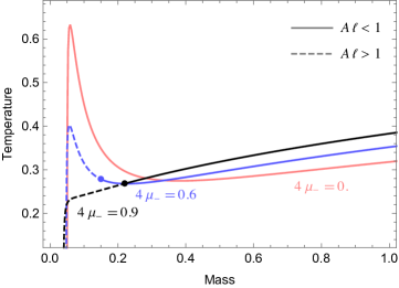
Figure 4: A plot of temperature as a function of mass for the charged black hole, with fixed $Q=0.05\ell$, and varying tension as labelled. As before, the slowly accelerating régime is shown as a solid line, and $A\ell>1$ is shown dashed.

We first explore the accelerating black hole in the canonical ensemble, i.e. where the charge, $Q$, of the black hole is fixed, but we allow $M$ and $\mu_{-}$ to vary. In figure 4, we give a representative plot of temperature as a function of black hole mass for $Q=0.05\ell$ to illustrate how increasing tension gradually removes the negative specific heat phase of the black hole.

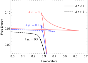
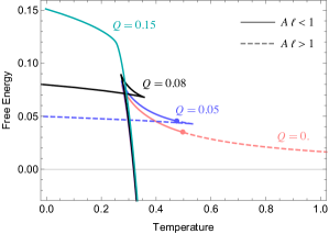
Figure 5: A plot of the free energy as a function of temperature for varying tension with $Q=0.05\ell$ on the left, and varying charge with $4\mu_{-}=0.3$ on the right.

Figure 5 shows the variation of the free energy $F=M-TS$ with temperature for varying tension and charge. As tension is increased, the swallowtail becomes smaller, and eventually disappears, analogous to the situation where the charge is gradually increased, shown on the right in figure 5. The free energy plot tells us that at low temperatures, we have the near extremal black hole, however as the mass of the black hole increases there is a critical value at which there is a spontaneous transition to a larger black hole with positive specific heat. The existence of this transition relies on the presence of the intermediate region of negative specific heat for the charged black hole. For large enough tension (or charge relative to $\ell$), there is a critical point at which this intermediate régime disappears, and the phase transition along with it. Figure 6 shows the “van der Waals” like behaviour of this coexistence curve for varying tension (in analogy to the varying potential plots of Chamblin:1999tk ), and cosmological constant (in analogy to Kubiznak:2012wp ).

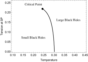
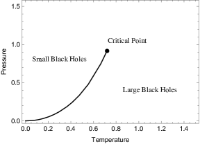
Figure 6: The coexistence line for the charged black hole shown for varying tension and cosmological constant with the black hole charge is fixed at $Q=0.05$. On the left, $\ell=1$, and the value of tension at the critical point is $\mu_{c}=0.219$. On the right, $4\mu_{-}=0.3$, and the critical value of the AdS radius is $\ell_{c}=0.36$.

Finally, for completeness we consider the thermodynamics of the accelerating charged black hole in the grand canonical ensemble, where we now allow charge to vary. The Gibbs potential is now $G=M-TS-Q\Phi$, with

$$\Phi=\Phi_{H}-\Phi_{0}=\frac{e}{r_{+}}-\frac{meA^{2}}{1+e^{2}A^{2}}$$ (49)

kept fixed. The interesting feature of fixed potential, as noted in Chamblin:1999tk for an isolated RNAdS black hole, is that there is a critical value of $\Phi$ delineating two qualitatively different behaviours of the black hole. For small fixed potentials, the charged AdS black hole can never approach extremality. This can be seen by noting that $f=f^{\prime}=0$ at extremality, where $f(r)$ is the RNAdS black hole potential. Solving these algebraic equations, and substituting $\Phi_{RN}=e/r_{+}$, one finds the constraint $3r_{+}^{2}/\ell^{2}=\Phi_{RN}^{2}-1$, thus for $|\Phi_{RN}|<1$ there is no possibility of extremality. In our case, for the charged accelerating black hole, the algebraic relations for extremality at fixed potential are considerably more complicated partly due to the extra acceleration parameter, but mostly because of the complicated expression for $\Phi$ (49). However, the same principle applies, and we also observe a similar phase transition from small to large $\Phi$, where the critical value of $\Phi$ is now tension dependent. Figure 7 demonstrates this behaviour showing the analogous plot to Chamblin:1999tk with acceleration for fixed $\mu_{-}$, and also how the behaviour depends on $\mu_{-}$ at fixed $\Phi$, illustrating how increasing $\mu_{-}$ improves the thermodynamic viability of the black hole. Figure 8 shows how the critical value of the potential, where only positive specific heat black holes are allowed, varies with tension.

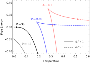
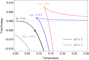
Figure 7: The Gibbs potential in the grand canonical ensemble as a function of temperature, on the left with $4\mu_{-}=0.3$ for varying potential as labelled, and on the right with $\Phi=0.9$ and varying tension as labelled in the plot.

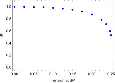
Figure 8: A plot of the critical value of $\Phi_{c}(\mu_{-})$ at which a black hole is always preferred for all temperatures as a function of the tension.

6 Conclusion

To sum up: we have shown how to allow for a varying conical deficit in black hole spacetimes, and found the relevant thermodynamical variables to describe the system. The appropriate first law has a varying tension term, with a thermodynamic length as its potential. This length consists of a direct geometrical part, a mass dependent correction, and finally, a shift in the presence of charge. The thermodynamic phases of accelerating black holes exhibit similar behaviour to their non-accelerating AdS cousins, however, the impact of acceleration is to improve the thermodynamic stability of the black holes.

It is interesting to note that the first law indicates that if the tension of a defect is fixed, then there is no contribution to the variation of $M$ coming from tension, yet, if the black hole increases its mass and hence its horizon radius, the horizon will now have consumed a portion of the string along each pole. This does not appear in the thermodynamic relation. This reinforces the interpretation of $M$ as the enthalpy of the black hole Kastor:2009wy . Although the black hole increases its internal energy by swallowing some cosmic string, it has also displaced the exact same amount of energy from the environment, resulting in no net overall gain in the total energy of the thermodynamic system (other than the mass that was added to the black hole in the first place).

It would be interesting to consider whether there are any holographic applications for these solutions. (See Anber:2008zz for a discussion of the CFT stress-energy at the background Rindler temperature.) Typically, one avoids having such distorted boundaries, however, the fact that the thermodynamics of these systems is now well defined perhaps suggests this is worth a second look.

Finally, we have not discussed rotating accelerating black holes here. Even for the non-accelerating rotating black hole, the thermodynamics are more subtle, requiring an adjustment of the angular velocity Gibbons:2004ai in order to define it relative to a non-rotating frame at infinity. For a conical defect running through the black hole (though see Gregory:2013xca ; Gregory:2014uca for a full discussion of subtleties of replacing deficits by finite width defects) one can follow the method of section 2 to generalise the appropriate thermodynamical variables of Gibbons et al. Gibbons:2004ai to:

$$M =\frac{m}{KL}\;\;\;;\;\;\;\; V =\frac{4\pi}{3}\left[\frac{r_{+}(r_{+}^{2}+a^{2})}{K}+a^{2}M\right]$$ (50)

$$J =\frac{am}{K^{2}}\;\;\;;\;\;\;\; \Omega =\Omega_{H}-\Omega_{\infty}=\frac{aK}{r_{+}^{2}+a^{2}}+\frac{aK}{\ell^{2}L}\;\;\;;\;\;\;\;$$

$$Q =\frac{e}{K}\;\;\;;\;\;\;\; \Phi =\frac{er_{+}}{r_{+}^{2}+a^{2}}$$

where $K$ is the (arbitrary) parameter determining the periodicity of the azimuthal angle as before, and $L$ is a new parameter due to black hole rotation:

$$L=1-\frac{a^{2}}{\ell^{2}}$$ (51)

In Gibbons:2004ai , $K=L$ was mandated by having no conical deficit on the rotation axis, however, here we are being more general. Allowing the tension of any deficit to vary leads to the thermodynamic length:

$$\lambda=\left(r_{+}-KM\frac{1+\frac{a^{2}}{\ell^{2}}}{1-\frac{a^{2}}{\ell^{2}}}\right)=\left(r_{+}-\frac{KM}{L}(2-L)\right)$$ (52)

Thus our black hole obeys a standard first law,

$$\delta M=T\delta S+V\delta P+\Omega\delta J+\Phi\delta Q-2\lambda\delta\mu$$ (53)

as well as a conventional Smarr relation:

$$M=2TS+\Phi Q-2PV+2\Omega J$$ (54)

Once the black hole is accelerating, it is no longer possible to have a completely non-rotating frame at infinity due to the distortion of the boundary. The potential therefore has a more complicated adjustment involving not only a shift, but also a decision on the appropriate frame to use at infinity. Computing the relevant parameters for the rotating accelerating black hole is underway.

References

- (1) M. Appels, R. Gregory and D. Kubizňák, Thermodynamics of Accelerating Black Holes, Phys. Rev. Lett. 117, no. 13, 131303 (2016) [arXiv:1604.08812 [hep-th]].
- (2) J. D. Bekenstein, Black holes and entropy, Phys. Rev. D 7, 2333 (1973).
- (3) J. D. Bekenstein, Generalized second law of thermodynamics in black hole physics, Phys. Rev. D 9, 3292 (1974).
- (4) S. W. Hawking, Particle Creation by Black Holes, Commun. Math. Phys. 43, 199 (1975) Erratum: [Commun. Math. Phys. 46, 206 (1976)].
- (5) R. Gregory and R. Laflamme, Black strings and p-branes are unstable, Phys. Rev. Lett. 70, 2837 (1993) [hep-th/9301052].
- (6) R. Gregory and R. Laflamme, The Instability of charged black strings and p-branes, Nucl. Phys. B 428, 399 (1994) [hep-th/9404071].
- (7) S. S. Gubser and I. Mitra, The Evolution of unstable black holes in anti-de Sitter space, JHEP 0108, 018 (2001) [hep-th/0011127].
- (8) H. S. Reall, Classical and thermodynamic stability of black branes, Phys. Rev. D 64, 044005 (2001) [hep-th/0104071].
- (9) S. Hollands and R. M. Wald, Stability of Black Holes and Black Branes, Commun. Math. Phys. 321, 629 (2013) [arXiv:1201.0463 [gr-qc]].
- (10) S. W. Hawking and D. N. Page, Thermodynamics of Black Holes in anti-De Sitter Space, Commun. Math. Phys. 87, 577 (1983).
- (11) E. Witten, Anti-de Sitter space, thermal phase transition, and confinement in gauge theories, Adv. Theor. Math. Phys. 2, 505 (1998) [hep-th/9803131].
- (12) H. Weyl, Zur Gravitationstheorie, Annalen der Physik 359, 117-145 (1917)
- (13) C. Charmousis and R. Gregory, Axisymmetric metrics in arbitrary dimensions, Class. Quant. Grav. 21, 527 (2004) [gr-qc/0306069].
- (14) W. Israel and K. A. Khan, Collinear particles and bondi dipoles in general relativity, Nuovo Cim. 33, 331 (1964)
- (15) H. F. Dowker and S. N. Thambyahpillai, Many accelerating black holes, Class. Quant. Grav. 20, 127 (2003) [gr-qc/0105044].
- (16) G. W. Gibbons and M. J. Perry, New Gravitational Instantons and Their Interactions, Phys. Rev. D 22, 313 (1980).
- (17) M. S. Costa and M. J. Perry, Interacting black holes, Nucl. Phys. B 591, 469 (2000) [hep-th/0008106].
- (18) C. Herdeiro, B. Kleihaus, J. Kunz and E. Radu, On the Bekenstein-Hawking area law for black objects with conical singularities, Phys. Rev. D 81, 064013 (2010) [arXiv:0912.3386 [gr-qc]].
- (19) G. W. Gibbons, Y. Pang and C. N. Pope, Thermodynamics of magnetized Kerr-Newman black holes, Phys. Rev. D 89, no. 4, 044029 (2014) [arXiv:1310.3286 [hep-th]].
- (20) M. Astorino, G. Comp re, R. Oliveri and N. Vandevoorde, Mass of Kerr-Newman black holes in an external magnetic field, Phys. Rev. D 94, no. 2, 024019 (2016) [arXiv:1602.08110 [gr-qc]].
- (21) I. Booth, M. Hunt, A. Palomo-Lozano and H. K. Kunduri, Insights from Melvin-Kerr-Newman spacetimes, Class. Quant. Grav. 32, no. 23, 235025 (2015) [arXiv:1502.07388 [gr-qc]].
- (22) W. Kinnersley and M. Walker, Uniformly accelerating charged mass in general relativity, Phys. Rev. D 2, 1359 (1970).
- (23) J. F. Plebanski and M. Demianski, Rotating, charged, and uniformly accelerating mass in general relativity, Annals Phys. 98, 98 (1976).
- (24) R. Gregory and M. Hindmarsh, Smooth metrics for snapping strings, Phys. Rev. D52 (1995) 5598–5605, [gr-qc/9506054].
- (25) K. Dutta, S. Ray and J. Traschen, Boost mass and the mechanics of accelerated black holes, Class. Quant. Grav. 23, 335 (2006) [hep-th/0508041].
- (26) M. Astorino, CFT Duals for Accelerating Black Holes, Phys. Lett. B 760, 393 (2016) [arXiv:1605.06131 [hep-th]].
- (27) M. Astorino, Thermodynamics of Regular Accelerating Black Holes, [arXiv:1612.04387 [gr-qc]].
- (28) A. Vilenkin, Cosmic strings and domain walls, Phys. Rep. 121 (1985) 263–315.
- (29) E. A. Martinez and J. W. York, Jr., Thermodynamics of black holes and cosmic strings, Phys. Rev. D 42, 3580 (1990).
- (30) M. Aryal, L. Ford, and A. Vilenkin, Cosmic strings and black holes, Phys. Rev. D34 (1986) 2263.
- (31) F. Bonjour, R. Emparan and R. Gregory, Vortices and extreme black holes: The Question of flux expulsion, Phys. Rev. D 59, 084022 (1999) [gr-qc/9810061].
- (32) R. Gregory, I. G. Moss and B. Withers, Black holes as bubble nucleation sites, JHEP 1403, 081 (2014) [arXiv:1401.0017 [hep-th]].
- (33) C. Teitelboim, The Cosmological Constant As A Thermodynamic Black Hole Parameter, Phys. Lett. 158B, 293 (1985).
- (34) D. Kastor, S. Ray and J. Traschen, Enthalpy and the Mechanics of AdS Black Holes, Class. Quant. Grav. 26, 195011 (2009) [arXiv:0904.2765 [hep-th]].
- (35) B. P. Dolan, The cosmological constant and the black hole equation of state, Class. Quant. Grav. 28, 125020 (2011) [arXiv:1008.5023 [gr-qc]].
- (36) M. Cvetic, G. W. Gibbons, D. Kubizňák and C. N. Pope, Black Hole Enthalpy and an Entropy Inequality for the Thermodynamic Volume, Phys. Rev. D 84, 024037 (2011) [arXiv:1012.2888 [hep-th]].
- (37) B. P. Dolan, Pressure and volume in the first law of black hole thermodynamics, Class. Quant. Grav. 28, 235017 (2011) [arXiv:1106.6260 [gr-qc]].
- (38) D. Kubizňák and R. B. Mann, P-V criticality of charged AdS black holes, JHEP 1207, 033 (2012) [arXiv:1205.0559 [hep-th]].
- (39) D. Kubizňák, R. B. Mann and M. Teo, Black hole chemistry: thermodynamics with Lambda, [arXiv:1608.06147 [hep-th]].
- (40) G. W. Gibbons, M. J. Perry and C. N. Pope, The First law of thermodynamics for Kerr-anti-de Sitter black holes, Class. Quant. Grav. 22, 1503 (2005) [hep-th/0408217].
- (41) A. Achucarro, R. Gregory, and K. Kuijken, Abelian Higgs hair for black holes, Phys. Rev. D52 (1995) 5729–5742, [gr-qc/9505039].
- (42) G. W. Gibbons and S. W. Hawking, Action Integrals and Partition Functions in Quantum Gravity, Phys. Rev. D 15, 2752 (1977)
- (43) L. Smarr, Mass formula for Kerr black holes, Phys. Rev. Lett. 30, 71 (1973) Erratum: [Phys. Rev. Lett. 30, 521 (1973)].
- (44) S. Lonsdale and I. Moss, The Motion of Cosmic Strings Under Gravity, Nucl. Phys. B 298, 693 (1988).
- (45) J. P. De Villiers and V. P. Frolov, Gravitational capture of cosmic strings by a black hole, Int. J. Mod. Phys. D 7, 957 (1998) [gr-qc/9711045].
- (46) O. J. C. Dias and J. P. S. Lemos, Pair of accelerated black holes in anti-de Sitter background: AdS C metric, Phys. Rev. D 67, 064001 (2003) [hep-th/0210065].
- (47) J. B. Griffiths and J. Podolsky, A New look at the Plebanski-Demianski family of solutions, Int. J. Mod. Phys. D 15, 335 (2006) [gr-qc/0511091].
- (48) J. Podolsky, Accelerating black holes in anti-de Sitter universe, Czech. J. Phys. 52, 1 (2002) [gr-qc/0202033].
- (49) K. Hong and E. Teo, A New form of the C metric, Class. Quant. Grav. 20, 3269 (2003) [gr-qc/0305089].
- (50) A. Magnon, On Komar integrals in asymptotically anti-de Sitter space-times, J. Math. Phys. 26, 3112 (1985).
- (51) R. Emparan, G. T. Horowitz and R. C. Myers, Exact description of black holes on branes, JHEP 0001, 007 (2000) [hep-th/9911043].
- (52) V. E. Hubeny, D. Marolf and M. Rangamani, Black funnels and droplets from the AdS C-metrics, Class. Quant. Grav. 27, 025001 (2010) [arXiv:0909.0005 [hep-th]].
- (53) P. Krtous, Accelerated black holes in an anti-de Sitter universe, Phys. Rev. D 72, 124019 (2005) [gr-qc/0510101].
- (54) D. Kastor and J. Traschen, The Angular Tension of Black Holes, Phys. Rev. D 86, 081501 (2012) [arXiv:1207.5415 [hep-th]].
- (55) J. H. Traschen and D. Fox, Tension perturbations of black brane space-times, Class. Quant. Grav. 21, 289 (2004) [gr-qc/0103106].
- (56) T. Harmark and N. A. Obers, General definition of gravitational tension, JHEP 0405, 043 (2004) [hep-th/0403103].
- (57) B. P. Dolan, Compressibility of rotating black holes, Phys. Rev. D 84, 127503 (2011) [arXiv:1109.0198 [gr-qc]].
- (58) A. Chamblin, R. Emparan, C. V. Johnson and R. C. Myers, Charged AdS black holes and catastrophic holography, Phys. Rev. D 60, 064018 (1999) [hep-th/9902170].
- (59) M. Cvetic and S. S. Gubser, Phases of R charged black holes, spinning branes and strongly coupled gauge theories, JHEP 9904, 024 (1999) [hep-th/9902195].
- (60) A. Chamblin, R. Emparan, C. V. Johnson and R. C. Myers, Holography, thermodynamics and fluctuations of charged AdS black holes, Phys. Rev. D 60, 104026 (1999) [hep-th/9904197].
- (61) M. M. Anber, AdS(4) / CFT(3) + Gravity for Accelerating Conical Singularities, JHEP 0811, 026 (2008) [arXiv:0809.2789 [hep-th]].
- (62) R. Gregory, D. Kubizňák and D. Wills, Rotating black hole hair, JHEP 1306, 023 (2013) [arXiv:1303.0519 [gr-qc]].
- (63) R. Gregory, P. C. Gustainis, D. Kubizňák, R. B. Mann and D. Wills, Vortex hair on AdS black holes, JHEP 1411, 010 (2014) [arXiv:1405.6507 [hep-th]].