Systematic Bias Due to Nonspinning Template Waveforms in the Gravitational Wave Parameter Estimation for Aligned-Spin Binary Black Holes

Abstract

We study the parameter estimation of gravitational waves for aligned-spin binary black hole (BBH) signals and assess the impact of bias that can be produced by using nonspinning template waveforms. We employ simple methods to calculate the statistical uncertainty from an overlap distribution. For the fiducial waveform model, we use a phenomenological model, which is designed to generate the gravitational waveforms emitted from merging BBH systems. We show that the mass parameters recovered by using nonspinning waveform templates can be significantly biased from the true values of aligned-spin signals. By comparing the systematic bias with the statistical uncertainty, we examine the validity of nonspinning templates for the parameter estimation of aligned-spin BBHs.

I INTRODUCTION

Since the prediction of gravitational radiation from Einstein’s general theory of relativity, no direct detection has been made for about 100 years because the gravitational wave (GW) strain is extremely weak. At last, however, two GW signals, named as GW150914 and GW151226, were recently detected by the two LIGO detectors GW1 ; GW2 , and future observing runs of the advanced detector network ALIGO ; AVirgo ; KAGRA are expected to yield more binary black hole (BBH) merger signals Aba10 ; Dom14 ; Abb16 ; Abb16b . Detailed analyses of the two GWs showed that both signals were emitted from merging BBHs GW1PE1 ; GW1PE2 ; GW2 . The masses of the two binaries were found to be $\sim 65M_{\odot}$ and $\sim 22M_{\odot}$ for GW150914 and GW151226, respectively. In particular, the masses of the two component BHs of GW150914 were estimated as $\sim 36M_{\odot}$ and $\sim 29M_{\odot}$, and those are believed to be the heaviest stellar-mass BHs known to date.

In GW data analyses for ground-based detectors, a GW event is identified in the search pipeline by using the matched filtering method All12 . Once a detection is made in the search, the parameter estimation pipeline seeks the physical properties of the GW source, such as mass and spin Aas13b . Generally, this procedure takes a very long time, up to several months depending on the waveform model used in the analysis Cor11 ; Vei12 ; Osh14a ; Osh14b . The result of the parameter estimation is given as probability density functions (PDFs) for all parameters and their correlations. The statistical uncertainty given in the PDF indicates how accurately the parameter can be measured by the analysis, and this measurement error depends on the strength of the GW signal. In principle, the statistical uncertainty is inversely proportional to the signal-to-noise ratio (SNR) Fin92 ; Cut94 . On the other hand, the result of the parameter estimation fundamentally includes another type of error, the systematic bias Cut07 . Unlike the statistical error, the systematic error relies on how exactly the wave function mimics real gravitational waveforms. For example, if a template waveform model neglects some physical parameters to simplify the wave function, this model cannot exactly describe real GW signals, and the parameter estimation analysis will give a wrong result. Typically, the validity of a waveform model used for the parameter estimation can be examined by comparing the systematic bias with the statistical uncertainty Fav14 ; Cho15d .

In this work, we investigate the statistical and the systematic errors in the parameter estimation for aligned-spin BBH signals. We adopt a simple approach to calculate the confidence region directly from an overlap distribution Bai13 and use the effective Fisher matrix method to determine the statistical uncertainty analytically Cho13 ; Cho14 . We calculate the bias that is produced by using nonspinning templates, and by comparing the biases with the statistical errors, we examine the validity of the templates in the parameter estimation for aligned-spin BBH signals. As our fiducial gravitational waveform model, we adopt a phenomenological model, which is an analytic approach designed to generate the gravitational waveforms emitted from aligned-spin BBH systems Kha16 .

II statistical error and systematic bias in the parameter estimation

The match between a detector data stream $x(t)$ and a template $h(t)$ can be defined as

$$\langle x|h\rangle=4{\rm Re}\int_{f_{\rm low}}^{\infty}\frac{\tilde{x}(f)\tilde{h}^{*}(f)}{S_{n}(f)}df,$$ (1)

where $S_{n}(f)$ is the power spectral density (PSD) of the detector noise, and $f_{\rm low}$ is the low-frequency cutoff that depends on the detector’s frequency band. The tilde denotes the Fourier transform of the time-domain waveform. In this work, we use the zero-detuned, high-power noise PSD, which is one of the designed sensitivities for Advanced LIGO apsd , and assume $f_{\rm low}=10$ Hz. For aligned-spin BBH systems in circular orbits, the wave function can be described by using 11 parameters: those are five extrinsic parameters (luminosity distance of the binary, two angles defining the sky position of the binary with respect to the detector, orbital inclination, and wave polarization), two arbitrary constants (coalescence time $t_{c}$ and coalescence phase $\phi_{c}$), and four intrinsic parameters (two masses $m_{1},m_{2}$ and two spins $\chi_{1},\chi_{2}$). However, the extrinsic parameters only scale the wave amplitude and do not affect our analysis. In addition, the contribution of the two arbitrary constants can be easily removed from our analysis by using certain analytic techniques All12 . Therefore, we consider only four parameters, $m_{1},m_{2},\chi_{1}$ and $\chi_{2}$, in our match calculation.

We define the overlap $P$ by the match between a normalized signal $\hat{h}_{s}$ and a normalized template $\hat{h}_{t}$ maximized over $t_{c}$ and $\phi_{c}$:

$$P=\max_{t_{c},\phi_{c}}\langle\hat{h}_{s}|\hat{h}_{t}\rangle.$$ (2)

If $\hat{h}_{s}=\hat{h}_{t}$, we obtain $P=1$. Since we take into account nonspinning templates in this work, the overlap function is distributed on the two-dimensional surface as

$$P(\lambda)=\max_{t_{c},\phi_{c}}\langle\hat{h}_{s}(\lambda_{0})|\hat{h}_{t}(\lambda)\rangle,$$ (3)

where $\lambda_{0}$ denotes a set of the true parameters of the signal, and $\lambda$ varies in the $m_{1}-m_{2}$ plane. In this equation, while the signal wave function has a spin parameter, the templates are nonspinning waveforms. Therefore, if the signal has a non-zero spin value, the mass parameters recovered by using the nonspinning templates can be systematically biased from the true parameters. The bias can be determined by the distance from the true value $\lambda_{0}$ to the recovered value $\lambda^{\rm rec}$:

$$b=\lambda^{\rm rec}-\lambda_{0}.$$ (4)

In the parameter estimation, the bias corresponds to the systematic error, and the magnitude of the bias is associated with the accuracy of the template waveform model. The impact of bias on the parameter estimation can be measured by comparing that with the statistical uncertainty. Below, we briefly describe how the statistical uncertainty can be calculated from the overlap distribution.

The PDF of the parameter estimation is given by the likelihood function ($L$), and the likelihood is related to the overlap as Cho13

$$\ln L(\lambda)=-\rho^{2}(1-P(\lambda)),$$ (5)

where $\rho$ is the SNR. From this relation, one can infer that the confidence region of the PDF is directly connected with a certain region in the overlap surface. Baird et al. Bai13 showed that if the likelihood has a Gaussian distribution, the confidence region is approximately consistent with the overlap region that is surrounded by the iso-match contour (IMC) determined by

$$P=1-{\chi^{2}_{k}(1-p)\over 2\rho^{2}},$$ (6)

where $\chi^{2}_{k}(1-p)$ is the chi-square value for which probability of obtaining that value or larger is $1-p$, and $k$ denotes the degree of freedom, which is given by the number of parameters. In this work, since we explore two-dimensional mass parameter space (i.e., $k=2$), the one-sigma confidence region (i.e., $p=0.682$) with $\rho=20$ is given by the contour $P=0.99714$.

Next, in order to calculate the statistical uncertainty and the correlation coefficient, we employ the Fisher matrix formalism (for more details refer to Val08 and references therein). The Fisher matrix can be calculated by using the overlap as Cho13 ; Cho14 ; Jar94

$$\Gamma_{ij}=\bigg{\langle}{\partial\tilde{h}\over\partial\lambda_{i}}\bigg{|}{\partial\tilde{h}\over\partial\lambda_{j}}\bigg{\rangle}\bigg{|}_{\lambda=\lambda_{0}}\simeq-\rho^{2}\frac{\partial^{2}P(\lambda)}{\partial\lambda_{i}\partial\lambda_{j}}\bigg{|}_{\lambda=\lambda_{0}}.$$ (7)

If the overlap surface has a quadratic shape, one can define a quadratic function $F$ that fits the overlap $P$. Using this function, Cho et al.Cho13 defined the effective Fisher matrix as

$$(\Gamma_{ij})_{\rm eff}=-\rho^{2}\frac{\partial^{2}F(\lambda)}{\partial\lambda_{i}\partial\lambda_{j}}\bigg{|}_{\lambda=\lambda_{0}}.$$ (8)

The inverse of $\Gamma_{ij}$ represents the covariance matrix of the parameter errors, and the statistical error ($\sigma_{i}$) of each parameter and the correlation coefficient ($c_{ij}$) between two parameters are determined by

$$\sigma_{i}=\sqrt{(\Gamma^{-1})_{ii}},\ \ \ {\cal C}_{ij}={(\Gamma^{-1})_{ij}\over\sqrt{(\Gamma^{-1})_{ii}(\Gamma^{-1})_{jj}}}.$$ (9)

On the other hand, if the waveform model is expressed by using an analytic function in the Fourier domain, such as in post-Newtonian models, the Fisher matrix can be directly computed from the wave function as in Eq. (7) Cho15a ; Cho15b ; Cho16 . However, the functional form of the phenomenological waveform model is much more complicated compared to the post-Newtonian models, so we adopt the effective Fisher matrix method in this work.

III phenomenological waveform model

The phenomenological waveform model is designed to produce the gravitational waveforms emitted from merging BBH systems. So far, various versions have been developed for nonspinning Aji07a ; Aji08a ; Aji08b , aligned-spin Aji11b ; San10 ; Kha16 , and precessing-spin Han14 systems. In this work, we use the most recent phenomenological model, the so-called PhenomD Kha16 . The phenomenological wave function defined in the Fourier domain has the form

$$\tilde{h}(f)=A_{\rm eff}(f)e^{i\Psi_{\rm eff}(f)},$$ (10)

where $A_{\rm eff}$ and $\Psi_{\rm eff}$ are the effective amplitude and the effective phase, and those are modeled separately and parameterized by using the mass and the spin parameters Cho15c .

On the other hand, for aligned-spin systems, the two spins are strongly correlated San10 ; Aji11a ; Pur13 ; Nie13 ; Pur16b . Thus, treating the effect of aligned-spins with a single spin parameter defined by

$$\chi\equiv\frac{m_{1}\chi_{1}+m_{2}\chi_{2}}{M},$$ (11)

is more efficient, where $M$ is the total mass. In the PhenomD wave function, the value of $\chi$ can be determined simply by choosing $\chi_{1}=\chi_{2}=\chi$. In this work, therefore, the signal waveforms are given by $h_{s}=h(m_{1},m_{2},\chi)=h_{\rm PhenomD}(m_{1},m_{2},\chi,\chi)$, and the template waveforms are given by $h_{t}=h(m_{1},m_{2})=h_{\rm PhenomD}(m_{1},m_{2},0,0)$ Cho16b . On the other hand, we use the chirp mass $M_{c}\equiv(m_{1}m_{2})^{3/5}/(m_{1}+m_{2})^{1/5}$ and the symmetric mass ratio $\eta\equiv m_{1}m_{2}/(m_{1}+m_{2})^{2}$ because those are more efficient than $m_{1},m_{2}$ in our analysis Cho15a .

IV Result

IV.1 Statistical Error

We choose five BBH signals with masses of $(30,5)M_{\odot}$, $(50,5)M_{\odot}$, $(50,10)M_{\odot}$, $(70,10)M_{\odot}$, and $(90,10)M_{\odot}$. Using Eq. (3), we calculate the overlap surfaces, where we have considered the signals with $\chi=0$ to obtain unbiased overlap surfaces. From the IMC approach given in Eq. (6), the one-sigma confidence region with $\rho=20$ can be given by the contour $P=0.99714$. On the other hand, the IMC method was established under the assumption that the PDF obeys a Gaussian distribution Bai13 . Thus, the accuracy of this method relies on the Gaussianity of the likelihood Has15 , and from Eq. (5), a Gaussian likelihood corresponds to a quadratic overlap in the region given by the SNR. Therefore, the confidence region obtained by using the IMC method can be reliable if the overlap surface has a quadratic shape in that region. To verify this, in Fig. 1, we show the confidence region (i.e., the contour of $P=0.99714$) and its fitting ellipse determined by using the quadratic fitting function $F$. One can see that the overlap contours almost exactly overlap their fitting ellipses. On the other hand, Berry et al. Ber15 investigated the effect of realistic non-Gaussian noises on the parameter estimation and found that the character of the noise made negligible difference to the PDFs.

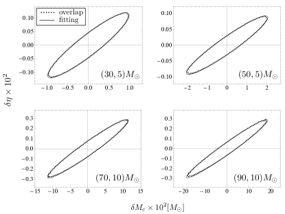
Figure 1: One-sigma confidence region with $\rho=20$ ($P=0.99714$), and its quadratic fitting ellipse.

Next, we calculate the effective Fisher matrix by inserting the fitting function $F$ into Eq. (8) and compute the statistical uncertainty and the correlation coefficient by using Eq. (9). In Table 1, we summarize the results for our BBH signals. Here, from the relation $M=M_{c}\eta^{-3/5}$, $\sigma_{M}$ can be computed in the following way:

$$\sigma_{M}^{2} = \left(\frac{\partial M}{\partial M_{c}}\right)^{2}\sigma_{M_{c}}^{2}+\left(\frac{\partial M}{\partial\eta}\right)^{2}\sigma_{\eta}^{2}$$

$$+2{\cal C}_{M_{c}\eta}\left(\frac{\partial M}{\partial M_{c}}\right)\left(\frac{\partial M}{\partial\eta}\right)\sigma_{M_{c}}\sigma_{\eta}.$$

We find that the fractional statistical errors ($\sigma_{\lambda}/\lambda$) for the mass parameters increase as the total mass increases. We also find that the correlation coefficient between $M_{c}$ and $\eta$ increases with increasing total mass, and this trend can be inferred from the ellipses in Fig. 1.

Table 1: Statistical uncertainties and correlation coefficients calculated by using the effective Fisher matrix method for BBH signals with $\rho=20$.

$m_{1}[M_{\odot}],\ m_{2}[M_{\odot}]$	30, 5	50, 5	50, 10	70, 10	90, 10
$\sigma_{M_{c}}/M_{c}\times 10^{2}$	0.065	0.110	0.250	0.359	0.520
$\sigma_{\eta}/\eta\times 10^{2}$	0.647	0.739	1.469	1.741	2.159
${\cal C}_{M_{c}\eta}$	0.921	0.944	0.952	0.963	0.973
$\sigma_{M}/M\times 10^{2}$	0.329	0.341	0.648	0.705	0.798

IV.2 Impact of the Systematic Bias

We now consider the spin for our signals and calculate the overlaps by using Eq. (3). Since our templates do not have spins, the resultant overlap surfaces are biased, and the bias can be measured by using Eq. (4). Basically, the templates cannot be reliable for the parameter estimation if the recovered parameter is significantly biased from the true parameter. To examine the validity of nonspinning templates for aligned-spin signals, we compare the systematic bias with the statistical uncertainty for the parameter $M$. The result is given in Fig. 2, where we have adopted the statistical uncertainties given in Table 1. We find that the systematic errors are much larger than the statistical errors, even with a very small value of the spin. In addition, the ratio $b/\sigma$ can be larger for higher SNRs because the statistical error is inversely proportional to the SNR. Therefore, we conclude that nonspinning templates are unsuitable for the parameter estimation for aligned-spin BBH signals. On the other hand, one can see a linear dependence of the ratio $b/\sigma$ on the spin in the range of $-0.4\leq\chi\leq 0.4$ for all signals. Interestingly, depending on the mass of the lighter BH rather than the total mass, the results in this figure show clearly separated populations. This is because the statistical error ($\sigma_{M}/M$) depends mainly on the mass of the lighter BH, as shown in Table 1, while the biases ($b_{M}/M$) are mostly consistent independently of the masses.

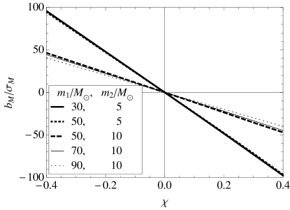
Figure 2: Comparison between the systematic bias ($b$) and the statistical uncertainty ($\sigma$) for the parameter $M$.

V Summary and Conclusion

We studied the reliability of nonspinning templates in the GW parameter estimation for aligned-spin BBH signals. Assuming several signals with various masses, we calculated the statistical uncertainty by using the IMC and the effective Fisher matrix methods. We also calculated the systematic biases induced by nonspinning templates for the aligned-spin signals and compared those with the statistical uncertainties to examine the impact of bias on the parameter estimation. We found that the total mass recovered by using the nonspinning templates could be significantly biased from the true value of the aligned-spin signal. The bias can exceed the statistical error even with a very small value of the spin. Therefore, nonspinning templates are unsuitable for the parameter estimation for aligned-spin BBH signals.

References

- (1) B. P. Abbott et al.(LIGO Scientific Collaboration and Virgo Collaboration), Phys. Rev. Lett. 116, 061102 (2016).
- (2) B. P. Abbott et al.(LIGO Scientific Collaboration and Virgo Collaboration), Phys. Rev. Lett. 116, 241103 (2016).
- (3) J. Aasi et al.(LIGO Scientific Collaboration), Classical Quantum Gravity 32, 074001 (2015).
- (4) F. Acernese et al., Classical Quantum Gravity 32, 024001 (2015).
- (5) Y. Aso, Y. Michimura, K. Somiya, M. Ando, O. Miyakawa, T. Sekiguchi, D. Tatsumi, and H. Yamamoto (The KAGRA Collaboration), Phys. Rev. D 88, 043007 (2013).
- (6) J. Abadie et al.(LIGO Scientific Collaboration and Virgo Collaboration), Classical Quantum Gravity 27, 173001 (2010).
- (7) M. Dominik, E. Berti, R. O’Shaughnessy, I. Mandel, K. Belczynski, C. Fryer, D. Holz, T. Bulik, and F. Pannarale, Astrophys. J. 806, 263 (2015).
- (8) B. P. Abbott et al.(LIGO Scientific Collaboration and Virgo Collaboration), Astrophys. J. Lett. 833, L1 (2016).
- (9) B. P. Abbott et al.(LIGO Scientific Collaboration and Virgo Collaboration), Phys. Rev. X 6, 041015 (2016).
- (10) B. P. Abbott et al.(LIGO Scientific Collaboration and Virgo Collaboration), Phys. Rev. Lett. 116, 241102 (2016).
- (11) B. P. Abbott et al.(LIGO Scientific Collaboration and Virgo Collaboration), Phys. Rev. X 6, 041014 (2016).
- (12) B. Allen, W. G. Anderson, P. R. Brady, D. A. Brown, and J. D. E. Creighton, Phys. Rev. D 85, 122006 (2012).
- (13) J. Aasi et al.(LIGO Scientific Collaboration and Virgo Collaboration), Phys. Rev. D 88, 062001 (2013).
- (14) N. Cornish, L. Sampson, N. Yunes, and F. Pretorius, Phys. Rev. D 84, 062003 (2011).
- (15) J. Veitch, I. Mandel, B. Aylott, B. Farr, V. Raymond, C. Rodriguez, M. V. van der Sluys, V. Kalogera, and A. Vecchio, Phys. Rev. D 85, 104045 (2012).
- (16) R. O’Shaughnessy, B. Farr, E. Ochsner, H.-S. Cho, C. Kim, and C.-H. Lee, Phys. Rev. D 89, 064048 (2014).
- (17) R. O’Shaughnessy, B. Farr, E. Ochsner, H.-S. Cho, V. Raymond, C. Kim, and C.-H. Lee, Phys. Rev. D 89, 102005 (2014).
- (18) L. S. Finn, Phys. Rev. D 46, 5236 (1992).
- (19) C. Cutler and É. E. Flanagan, Phys. Rev. D 49, 2658 (1994).
- (20) C. Cutler and M. Vallisneri, Phys. Rev. D 76, 104018 (2007).
- (21) M. Favata, Phys. Rev. Lett. 112, 101101 (2014).
- (22) H.-S. Cho, Classical Quantum Gravity 32, 235007 (2015).
- (23) E. Baird, S. Fairhurst, M. Hannam, and P. Murphy, Phys. Rev. D 87, 024035 (2013).
- (24) H.-S. Cho, E. Ochsner, R. O’Shaughnessy, C. Kim, and C.-H. Lee, Phys. Rev. D 87, 024004 (2013).
- (25) H.-S. Cho and C.-H. Lee, Classical Quantum Gravity 31, 235009 (2014).
- (26) S. Khan, S. Husa, M. Hannam, F. Ohme, M. Pürrer, X. J. Forteza, and A. Bohé, Phys. Rev. D 93, 044007 (2016).
- (27) Advanced LIGO anticipated sensitivity curves, https://dcc.ligo.org/LIGO-T0900288/public.
- (28) M. Vallisneri, Phys. Rev. D 77, 042001 (2008).
- (29) P. Jaranowski and A. Królak, Phys. Rev. D 49, 1723 (1994).
- (30) H.-S. Cho, J. Korean Phys. Soc. 66, 1637 (2015).
- (31) H.-S. Cho, J. Korean Phys. Soc. 67, 960 (2015).
- (32) H.-S. Cho, J. Korean Phys. Soc. 69, 884 (2016).
- (33) P. Ajith et al., Classical Quantum Gravity 24, S689 (2007).
- (34) P. Ajith et al., Phys. Rev. D 77, 104017 (2008); 79, 129901(E) (2009).
- (35) P. Ajith, Classical Quantum Gravity 25, 114033 (2008).
- (36) P. Ajith et al., Phys. Rev. Lett. 106, 241101 (2011).
- (37) L. Santamaria et al., Phys. Rev. D 82, 064016 (2010).
- (38) M. Hannam, P. Schmidt, A. Bohé, L. Haegel, S. Husa, F. Ohme, G. Pratten, and M. Pürrer, Phys. Rev. Lett. 113, 151101 (2014).
- (39) H.-S. Cho, Classical Quantum Gravity 32, 215023 (2015).
- (40) P. Ajith, Phys. Rev. D 84, 084037 (2011).
- (41) M. Pürrer, M. Hannam, P. Ajith, and S. Husa, Phys. Rev. D 88, 064007 (2013).
- (42) A. B. Nielsen, Classical Quantum Gravity 30, 075023 (2013).
- (43) M. Pürrer, M. Hannam, and F. Ohme, Phys. Rev. D 93, 084042 (2016).
- (44) H.-S. Cho, Phys. Rev. D 94, 124045 (2016).
- (45) C.-J. Haster, I. Mandel, and W. M. Farr, Classical Quantum Gravity 32, 235017 (2015).
- (46) C. P. L. Berry, et al., Astrophys. J. 804, 114 (2015).