Effective radius of ground- and excited-state positronium in collisions with hard walls

Abstract

We determine effective collisional radii of positronium (Ps) by considering Ps states in hard-wall spherical cavities. $B$-spline basis sets of electron and positron states inside the cavity are used to construct the states of Ps. Accurate Ps energy eigenvalues are obtained by extrapolation with respect to the numbers of partial waves and radial states included in the bases. Comparison of the extrapolated energies with those of a pointlike particle provides values of the effective radius $\rho_{nl}$ of Ps($nl$) in collisions with a hard wall. We show that for $1s$, $2s$, and $2p$ states of Ps, the effective radius decreases with the increasing Ps center-of-mass momentum, and find $\rho_{1s}=1.65$ a.u., $\rho_{2s}=7.00$ a.u., and $\rho_{2p}=5.35$ a.u. in the zero-momentum limit.

I Introduction

Positronium (Ps) is a light atom that consists of an electron and its antiparticle, the positron. Positron- and positronium-annihilation-lifetime spectroscopy is a widely used tool for studying materials, e.g., for determining pore sizes and free volume. For smaller pores the radius of the Ps atom itself cannot be neglected. This quantity was probed in a recent experiment which measured the cavity shift of the Ps $1s$-$2p$ line Cassidy et al. (2011), and the data calls for proper theoretical understanding Green and Gribakin (2011). In this paper we calculate the eigenstates of Ps in a hard-wall spherical cavity and determine the effective collisional radius of Ps in $1s$, $2s$, and $2p$ states as a function of its center-of-mass momentum.

The most common model for pore-size estimation is the Tao-Eldrup model Tao (1972); Eldrup et al. (1981). It considers an orthopositronium atom ($o$-Ps), i.e., a Ps atom in the triplet state, confined in the pore which is assumed to be spherical, with radius $R_{c}$. The Ps is modeled as a point particle with mass $2m_{e}$ in a spherical potential well, where $m_{e}$ is the mass of an electron/positron. Collisions of $o$-Ps with the cavity walls allow for positron two-gamma ($2\gamma$) annihilation with the electrons in the wall, which reduces the $o$-Ps lifetime with respect to the vacuum $3\gamma$-annihilation value of 142 ns. To simplify the description of the penetration of the Ps wave function into the cavity wall, the radius of the potential well is taken to be $R_{c}+\Delta R_{c}$, where the best value of $\Delta R_{c}$ has been empirically determined to be 0.165 nm Schrader and Jean (1988). The model and its extensions are still widely used for pore sizes in 1–100 nm range Gidley et al. (1999); Goworek et al. (2002); Wada and Hyodo (2013).

Porous materials and Ps confinement in cavities also enabled a number of fundamental studies, such as measurement of Ps-Ps interactions Cassidy and Mills, Jr. (2011), detection of the Ps₂ molecule Cassidy and Mills, Jr. (2007a) and its optical spectroscopy Cassidy et al. (2012), and measurements of the cavity-induced shift of the Ps Lyman-$\alpha$ ($1s$-$2p$) transition Cassidy et al. (2011). Cavities also hold prospects of creating a Bose-Einstein condensate of Ps atoms and an annihilation-gamma-ray laser Cassidy and Mills, Jr. (2007b).

Seen in a wider context, the old subject of confined atoms Michels et al. (1937); Sommerfeld and Welker (1938) has seen renewed interest in recent years Jaskólski (1996); Buchachenko (2001); Connerade and Kengkan (2003, 2005); Sabin and Brandas (2009a, b). Studies in this area not only serve as interesting thought experiments but also apply to real physical situations, e.g., atoms under high pressure Lawrence et al. (1981); Connerade and Semaoune (2000) or atoms trapped in fullerenes Bethune et al. (1993); Shinohara (2000); Komatsu et al. (2005). For $o$-Ps there is a specific question about the extent to which confinement in a cavity affects its intrinsic $3\gamma$ annihilation rate (see Ref. Marlotti Tanzi et al. (2016) and references therein).

For smaller cavities the effect of a finite radius of the trapped particle on its center-of-mass motion cannot be ignored. In fact, the radius of a composite quantum particle depends on the way this quantity is defined and probed. For example, the proton is usually characterized by its root-mean-squared charge radius. It is measured in elastic electron-proton scattering Bernauer et al. (2010) or using spectroscopy of exotic atoms, such as muonic hydrogen Antognini et al. (2013) (with as yet unexplained discrepancies between these experiments). For a particle trapped in a cavity, any practically defined radius may depend on the nature of its interaction with the walls.

In the present work we consider the simple problem of a Ps atom confined in a hard-wall spherical cavity. The finite size of Ps gives rise to energy shifts with respect to the energy levels of a pointlike particle in the cavity. This allows us to calculate the effective collisional radius of Ps that describes its interaction with the impenetrable cavity wall.

Ps is a hydrogenlike atom with a total mass of 2 and reduced mass of $\frac{1}{2}$ (in atomic units). The most probable distance between the electron and positron in a free ground-state Ps atom is $2a_{0}$, where $a_{0}$ is the Bohr radius, while the mean electron-positron separation is $3a_{0}$ Landau and Lifshitz (1965). For excited states Ps$(nl$) these quantities increase as $n^{2}$. The Ps center of mass is halfway between the two particles, so the most probable radius of Ps($1s$) is $1a_{0}$, its mean radius being $1.5a_{0}$. One can expect that the distance of closest approach between the Ps center of mass and the wall with which it collides will be similar to these values. One can also expect that this distance will depend on the center-of-mass momentum of the Ps atom, as it will be “squashed” when colliding with the wall at higher velocities.

A proper quantum-mechanical treatment of this problem is the subject of this work. A configuration-interaction (CI) approach with a $B$-spline basis is used to construct the states of Ps inside the cavity. Using these we determine the dependence of the effective Ps radius on the center-of-mass momentum for the $1s$, $2s$, and $2p$ states.

Of course, the interaction between Ps and cavity walls in real materials is different from the idealized situation considered here. It can be modeled by changing the electron-wall and positron-wall potentials. On the other hand, the hard-wall cavity can be used as a theoretical tool for studying Ps interactions with atoms Swann and Gribakin (2017). An atom placed at the center of the cavity will cause a shift of the Ps energy levels, whose positions can be related to the Ps-atom scattering phase shifts $\delta_{L}(K)$ for the $L$th partial wave Burke (1977),

$$\tan\delta_{L}(K)=\frac{J_{L+1/2}(K[R_{c}-\rho(K)])}{Y_{L+1/2}(K[R_{c}-\rho(K)])},$$ (1)

where $K$ is the Ps center-of-mass momentum, $J_{\nu}$ is the Bessel function, $Y_{\nu}$ is the Neumann function, $R_{c}$ is the cavity radius, and $\rho(K)$ is the effective collisional radius of the Ps atom.

The paper is organized as follows. Section II describes the theory and numerical implementation of the CI calculations of the energy levels and effective radii of Ps in a spherical cavity. In Sec. III these energies and radii are presented for a number of cavity sizes and the dependence of the radii of Ps($1s$), Ps($2s$), and Ps($2p$) on the Ps center-of-mass momentum is analyzed. We conclude in Sec. IV with a summary.

Unless otherwise stated, atomic units are used throughout.

II Theory and numerical implementation

II.1 Ps states in the cavity

The radial parts of the electron and positron states in an empty spherical cavity with impenetrable walls are solutions of the Schrödinger equation

$${-}\frac{1}{2}\frac{d^{2}P_{\varepsilon l}}{dr^{2}}+\frac{l(l+1)}{2r^{2}}P_{\varepsilon l}(r)=\varepsilon P_{\varepsilon l}(r),$$ (2)

where $l$ is the orbital angular momentum, that satisfy the boundary conditions $P_{\varepsilon l}(0)=P_{\varepsilon l}(R_{c})=0$. Although Eq. (2) has analytical solutions, we obtain the solutions numerically by expanding them in a $B$-spline basis,

$$P_{\varepsilon l}(r)=\sum_{i}C_{i}B_{i}(r),$$ (3)

where $B_{i}(r)$ are the $B$ splines, defined on an equispaced knot sequence de Boor (2001). A set of 40 splines of order 6 has been used throughout. Using $B$ splines has the advantange that a central atomic potential can be added in Eq. (2) to investigate Ps-atom interactions Swann and Gribakin (2017).

We denote the electron states by $\phi_{\mu}(\mathbf{r}_{e})=r_{e}^{-1}P_{\varepsilon l}(r_{e})Y_{lm}(\Omega_{e})$, where $Y_{lm}(\Omega)$ is the spherical harmonic that depends on the spherical angles $\Omega$, and the positron states by $\phi_{\nu}(\mathbf{r}_{p})$, where $\mathbf{r}_{e}$ ($\mathbf{r}_{p}$) is the position vector of the electron (positron) relative to the center of the cavity. For Ps in an empty cavity the two sets of states are identical. The indices $\mu$ and $\nu$ stand for the possible orbital angular momentum and radial quantum numbers of each state.

The nonrelativistic Hamiltonian for Ps inside the cavity is

$$H=-\frac{1}{2}\nabla_{e}^{2}-\frac{1}{2}\nabla_{p}^{2}+V(\mathbf{r}_{e},\mathbf{r}_{p}),$$ (4)

where $V(\mathbf{r}_{e},\mathbf{r}_{p})=-|\mathbf{r}_{e}-\mathbf{r}_{p}|^{-1}$ is the Coulomb interaction between the electron and positron. The infinite potential of the wall is taken into account through the boundary conditions at $r_{e}=r_{p}=R_{c}$. The Ps wave functions with a given total angular momentum $J$ and parity $\Pi$ are constructed as

$$\Psi_{J\Pi}(\mathbf{r}_{e},\mathbf{r}_{p})=\sum_{\mu,\nu}C_{\mu\nu}\phi_{\mu}(\mathbf{r}_{e})\phi_{\nu}(\mathbf{r}_{p}),$$ (5)

where the $C_{\mu\nu}$ are coefficients. The sum in Eq. (5) is over all allowed values of the orbital and radial quantum numbers up to infinity. Numerical calculations employ finite values of $l_{\text{max}}$ and $n_{\text{max}}$, respectively, and we use extrapolation to achieve completeness (see below).

Substitution of Eq. (5) into the Schrödinger equation

$$H\Psi_{J\Pi}=E\Psi_{J\Pi},$$ (6)

leads to a matrix-eigenvalue problem

$$\mathbf{H}\mathbf{C}=E\mathbf{C},$$ (7)

where the Hamiltonian matrix $\mathbf{H}$ has elements

$$\langle\nu^{\prime}\mu^{\prime}|H|\mu\nu\rangle=(\varepsilon_{\mu}+\varepsilon_{\nu})\delta_{\mu\mu^{\prime}}\delta_{\nu\nu^{\prime}}+\langle\nu^{\prime}\mu^{\prime}|V|\mu\nu\rangle,$$ (8)

$\varepsilon_{\mu}$ ($\varepsilon_{\nu}$) is the energy of the single-particle state $\mu$ ($\nu$), and $\langle\nu^{\prime}\mu^{\prime}|V|\mu\nu\rangle$ is the electron-positron Coulomb matrix element. The vector $\mathbf{C}$ contains the expansion coefficients $C_{\mu\nu}$. Diagonalization of the Hamiltonian matrix yields the energy eigenvalues $E$ and the expansion coefficients. Working expressions for the wave function and matrix elements, in which the radial and angular variables are separated, are shown in Appendix A.

II.2 Definition of the Ps effective radius

The effective Ps radius is determined from the energy shifts with respect to the states of a point particle with the same mass as Ps. We employ the notation $nl[N,L]$ to label the states of Ps in the cavity. Here $nl$ refers to its internal state, and $[N,L]$ describes the state of the Ps center-of-mass motion. The means of determining the four quantum numbers $n$, $l$, $N$, and $L$ for Ps states is described in Sec. II.3. Also, to obtain accurate values of the effective Ps radius, the energy eigenvalues $E$ and other expectation values are extrapolated to the limits $l_{\text{max}}\to\infty$ and $n_{\text{max}}\to\infty$; this is discussed in detail in Sec. II.4.

We consider each energy eigenvalue $E_{nl[N,L]}$ as the sum

$$E_{nl[N,L]}=E_{nl}^{\text{int}}+E_{nl[N,L]}^{\text{COM}},$$ (9)

where $E_{nl}^{\text{int}}=-1/4n^{2}$ is the internal Ps bound-state energy, and $E_{nl[N,L]}^{\text{COM}}$ is the energy of the center-of-mass motion. The latter is related to the center-of-mass momentum $K_{nl[N,L]}$ by

$$E_{nl[N,L]}^{\text{COM}}=\frac{K_{nl[N,L]}^{2}}{2m},$$ (10)

where $m=2$ is the mass of Ps.

Away from the wall the Ps wave function decouples into separate internal and center-of-mass wave functions, viz.,

$$\Psi_{J\Pi}(\mathbf{r},\mathbf{R})\simeq\sum_{m,M_{L}}C^{JM}_{lmLM_{L}}\psi_{nlm}^{\text{int}}(\mathbf{r})\Phi_{nl[N,L]}^{\text{COM}}(\mathbf{R}),$$ (11)

where $\mathbf{r}=\mathbf{r}_{e}-\mathbf{r}_{p}$, $\mathbf{R}=(\mathbf{r}_{e}+\mathbf{r}_{p})/2$ is the position vector of the Ps center of mass, and $C^{JM}_{lmLM_{L}}$ is the Clebsch-Gordan coefficient that couples the rotational state $lm$ of the Ps internal motion with that of its center-of-mass motion ($LM_{L}$). Since the center of mass is in free motion, its wave function is given by

$$\Phi_{nl[N,L]}^{\text{COM}}(\mathbf{R})\propto\frac{1}{\sqrt{R}}J_{L+1/2}(K_{nl[N,L]}R)Y_{LM_{L}}(\Omega_{\mathbf{R}}).$$ (12)

For a pointlike particle, the quantization of the radial motion in the hard-wall cavity of radius $R_{c}$ gives $K_{nl[N,L]}R_{c}=z_{L+1/2,N}$, where $z_{L+1/2,N}$ is the $N$th positive root of the Bessel function $J_{L+1/2}(z)$. (For $S$-wave Ps, $L=0$, $z_{1/2,N}=\pi N$.) When the finite effective radius $\rho_{nl[N,L]}$ of the Ps atom is taken into account, one has

$$K_{nl[N,L]}(R_{c}-\rho_{nl[N,L]})=z_{L+1/2,N},$$ (13)

which gives the energy (9) as

$$E_{nl[N,L]}=-\frac{1}{4n^{2}}+\frac{z_{L+1/2,N}^{2}}{4(R_{c}-\rho_{nl[N,L]})^{2}}.$$ (14)

This relation defines the effective collisional radius of Ps,

$$\rho_{nl[N,L]}=R_{c}-z_{L+1/2,N}\mathopen{}\mathclose{{}\left(4E_{nl[N,L]}+\frac{1}{n^{2}}}\right)^{-1/2}.$$ (15)

The Ps radius thus defined may depend on the Ps center-of-mass state $[N,L]$, as well as the cavity radius. As we show in Sec. III, the radius is in fact determined only by the internal Ps state $nl$ and its center-of-mass momentum $K$, i.e., it can be written as $\rho_{nl}(K)$.

In the present work, most of the calculations were performed for $J^{\Pi}=0^{+}$ and $1^{-}$, and cavity radii $R_{c}=10$ a.u. and 12 a.u. The value of $R_{c}$ was kept small to assist convergence of the CI expansion (5).

II.3 Identification of Ps states

After diagonalizing the Hamiltonian matrix and finding the energy eigenvalues, one must determine the quantum numbers for each state before the corresponding Ps radius $\rho_{nl[N,L]}$ can be calculated from Eq. (15). To facilitate this, the mean electron-positron separation $\langle r\rangle$ and contact density $\langle\delta(\mathbf{r})\rangle$ were calculated for each state (see Appendix A for details).

The value of $\langle r\rangle$ for free Ps is twice the hydrogenic electron radius Landau and Lifshitz (1965),

$$\langle r\rangle=3n^{2}-l(l+1).$$ (16)

Thus, the expected mean separations for the $1s$, $2s$, and $2p$ states are 3, 12, and 10 a.u., respectively. In practice, the calculated separations for the $2s$ and $2p$ states are noticeably lower (see Sec. II.4.2), since the free-Ps values of $\langle r\rangle$ are comparable to the size of the cavity. Nevertheless, they are useful for identifying the individual Ps states.

The contact density $\langle\delta(\mathbf{r})\rangle$ is useful for distinguishing between $s$ and $p$ states, and between the $s$ states with different principal quantum number $n$. For $s$ states of free Ps, the contact density is given by the hydrogenic electron density at the origin Landau and Lifshitz (1965) scaled by the cube of the reduced-mass factor, viz.,

$$\langle\delta(\mathbf{r})\rangle=\frac{1}{8\pi n^{3}}.$$ (17)

Hence, the expected contact densities of $1s$ and $2s$ states are $1/8\pi\approx 0.04$ and $1/64\pi\approx 5\times 10^{-3}$, respectively. For $p$ and higher-angular-momentum states the contact density is zero. In practice, the computed contact density for a $p$ state was observed to be of the order of $10^{-8}$ or smaller.

Although looking at the numerical values of $\langle r\rangle$ and $\langle\delta(\mathbf{r})\rangle$ calculated for finite $l_{\text{max}}$ and $n_{\text{max}}$ is often sufficient for distinguishing between the various states, their values can also be extrapolated to the limits $l_{\text{max}}\to\infty$ and $n_{\text{max}}\to\infty$, as demonstrated in Sec. II.4.

Once the internal Ps state $nl$ has been established using the mean electron-positron separation and contact density, the angular momentum and parity selection rules,

$$|l-L|\leq J\leq l+L,$$ (18)

$$\Pi=(-1)^{l+L},$$ (19)

allow one to determine the possible values of $L$.

Finally, for fixed $n$, $l$, and $L$, with the energy eigenvalues arranged in increasing numerical order, the corresponding values of $N$ are 1, 2, 3, etc.

II.4 Extrapolation

II.4.1 Energy eigenvalues

In order to obtain the most precise values possible, the calculated energy eigenvalues are extrapolated to the limits $l_{\text{max}}\to\infty$ and $n_{\text{max}}\to\infty$. To this end, each calculation was performed for several consecutive values of $l_{\text{max}}$ with fixed $n_{\text{max}}$, and this process was repeated for several values of $n_{\text{max}}$. For $J^{\Pi}=0^{+}$ we used values of $l_{\text{max}}=11$–15 and $n_{\text{max}}=10$–15. Due to computational restrictions , for $J^{\Pi}=1^{-}$ it was necessary to lower the values of $l_{\text{max}}$ to the range 10–14, while keeping $n_{\text{max}}=10$–15 (Sec. II.5). Extrapolation is first performed with respect to $l_{\text{max}}$ for each value of $n_{\text{max}}$, and afterwards with respect to $n_{\text{max}}$.

The convergence of CI expansions of the type (5) is controlled by the Coulomb interaction between the particles. In our case, for $s$ states the contributions to the total energy from electron and positron states with orbital angular momentum $l$ behave as $(l+\frac{1}{2})^{-4}$, while for $p$ states, as $(l+\frac{1}{2})^{-6}$ Kutzelnigg and Morgan (1992); Gribakin and Ludlow (2002). Denoting by $E(l_{\text{max}},n_{\text{max}})$ a generic unextrapolated energy eigenvalue computed with partial waves up to $l_{\rm max}$ with $n_{\max}$ states in each, we can extrapolate in $l_{\text{max}}$ by using fitting curves of the form

$$E(l_{\text{max}},n_{\text{max}}) =E(\infty,n_{\text{max}})+A\mathopen{}\mathclose{{}\left(l_{\text{max}}+\tfrac{1}{2}}\right)^{-3}$$

$$\quad{}+B\mathopen{}\mathclose{{}\left(l_{\text{max}}+\tfrac{1}{2}}\right)^{-4}+C\mathopen{}\mathclose{{}\left(l_{\text{max}}+\tfrac{1}{2}}\right)^{-5}$$ (20)

for $s$ states, and

$$E(l_{\text{max}},n_{\text{max}}) =E(\infty,n_{\text{max}})+A\mathopen{}\mathclose{{}\left(l_{\text{max}}+\tfrac{1}{2}}\right)^{-5}$$

$$\quad{}+B\mathopen{}\mathclose{{}\left(l_{\text{max}}+\tfrac{1}{2}}\right)^{-6}$$ (21)

for $p$ states, where $A$, $B$, and $C$ are fitting parameters, and higher-order terms are added to improve the fit. Such curves were found to give excellent fits for our data points. Figure 1 shows the extrapolation of the 6 lowest energy eigenvalues for $J^{\Pi}=0^{+}$, $R_{c}=10$ a.u., and $n_{\text{max}}=15$. The effect of extrapolation can be seen better in Fig. 2, which shows it for the lowest eigenvalue.

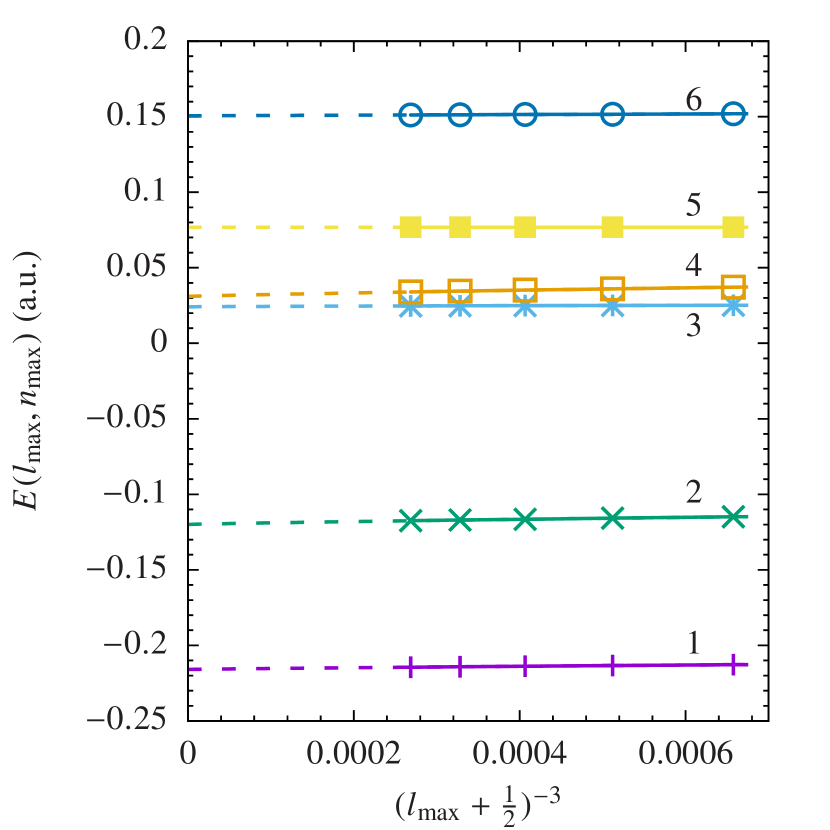
Figure 1: Extrapolation in $l_{\text{max}}$ for the lowest 6 energy eigenvalues for $J^{\Pi}=0^{+}$, $R_{c}=10$ a.u., and $n_{\text{max}}=15$. Solid lines connect the data points to guide the eye, while the dashed lines show extrapolation to $l_{\rm max}\rightarrow\infty$ using Eq. (II.4.1) or (II.4.1).

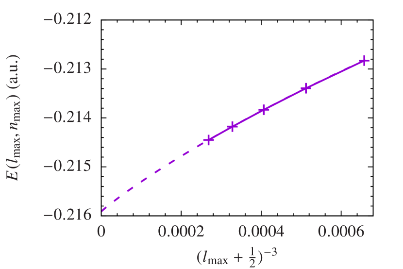
Figure 2: Extrapolation in $l_{\text{max}}$ for the lowest energy eigenvalue for $J^{\Pi}=0^{+}$, $R_{c}=10$ a.u., and $n_{\text{max}}=15$. The solid line connects the data points to guide the eye, while the dashed line shows extrapolation to $l_{\rm max}\rightarrow\infty$ using Eq. (II.4.1).

To extrapolate with respect to the maximum number of states in each partial wave, we assume that the increments in the energy with increasing $n_{\rm max}$ decrease as its negative power. The extrapolated energy eigenvalue $E_{nl[N,L]}$ is then found from the fit

$$E(\infty,n_{\text{max}})=E_{nl[N,L]}+\alpha n_{\text{max}}^{-\beta},$$ (22)

where $\alpha$ and $\beta$ are fitting parameters. Again, such curves produced very good fits for our data points. Figure 3 shows the extrapolation of the 6 lowest energy eigenvalues for $J^{\Pi}=0^{+}$ and $R_{c}=10$ a.u.

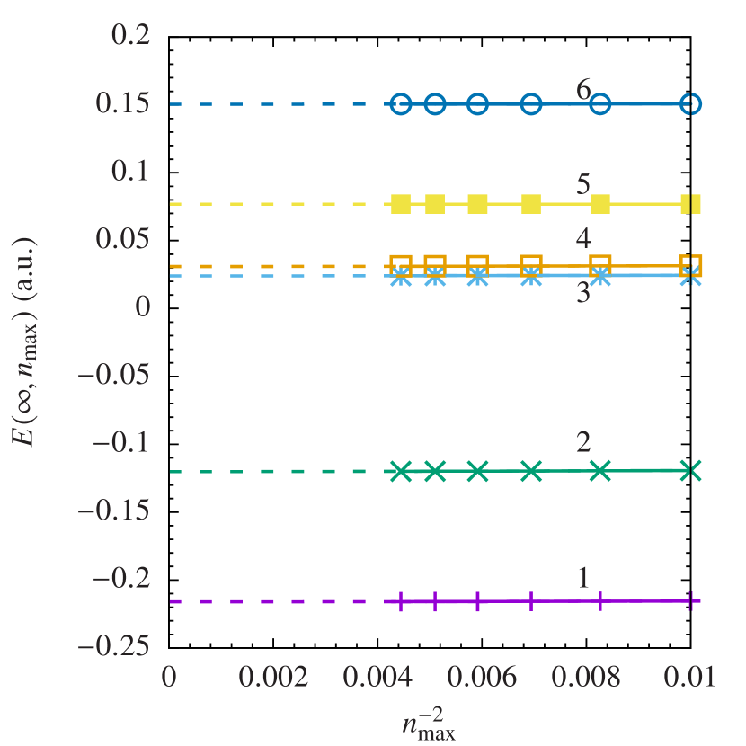
Figure 3: Extrapolation of the energy in $n_{\text{max}}$ for the lowest 6 energy eigenvalues for $J^{\Pi}=0^{+}$ and $R_{c}=10$ a.u. Solid lines connect the data points to guide the eye, while the dashed lines show extrapolation to $n_{\rm max}\rightarrow\infty$ using Eq. (22).

It is known that CI-type or many-body-theory calculations for systems containing Ps (either real or virtual) exhibit slow convergence with respect to the number of partial waves included Bray and Stelbovics (1993); Gribakin and Ludlow (2004); Mitroy and Bromley (2006); Zammit et al. (2013); Green and Gribakin (2013); Green et al. (2014). Accordingly, the extrapolation in $l_{\text{max}}$ is much more important than the extrapolation in $n_{\text{max}}$, which provides only a relatively small correction. This can be seen in Table 1, which shows the final extrapolated energy eigenvalues $E_{nl[N,L]}$ together with $E(\infty,n_{\text{max}})$ and $E(l_{\text{max}},n_{\text{max}})$ obtained for the largest $l_{\text{max}}$ and $n_{\text{max}}$ values.

II.4.2 Electron-positron separation

Expectation values of the electron-positron separation $\langle r\rangle$ and contact density $\langle\delta(\mathbf{r})\rangle$ can also be extrapolated to the limits $l_{\text{max}}\to\infty$ and $n_{\text{max}}\to\infty$. As with the energy, the extrapolation in $n_{\text{max}}$ makes only a small correction, which makes it superfluous here. We only use these quantities to identify Ps states, so precise values are not needed.

For the mean separation we used fits of the form

$$\langle r\rangle^{[l_{\rm max}]}=\langle r\rangle+A\mathopen{}\mathclose{{}\left(l_{\text{max}}+\tfrac{1}{2}}\right)^{-2}+B\mathopen{}\mathclose{{}\left(l_{\text{max}}+\tfrac{1}{2}}\right)^{-3}$$ (23)

for $s$ states, and

$$\langle r\rangle^{[l_{\rm max}]}=\langle r\rangle+A\mathopen{}\mathclose{{}\left(l_{\text{max}}+\tfrac{1}{2}}\right)^{-4}+B\mathopen{}\mathclose{{}\left(l_{\text{max}}+\tfrac{1}{2}}\right)^{-5}$$ (24)

for $p$ states, where $\langle r\rangle^{[l_{\rm max}]}$ is the value obtained in the calculation with a given $l_{\rm max}$. Figure 4 shows this extrapolation for $J^{\Pi}=0^{+}$, $R_{c}=10$ a.u., and $n_{\text{max}}=15$ for the 6 lowest energy eigenvalues, along with tentative identifications of the quantum numbers $n$ and $l$.

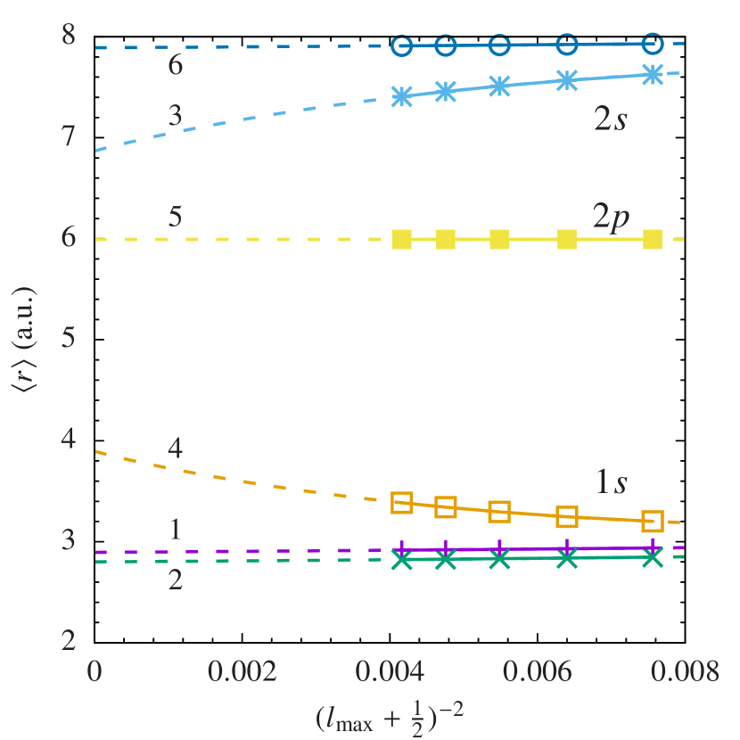
Figure 4: Extrapolation of the expected electron-positron separation in $l_{\text{max}}$ for the lowest 6 energy eigenvalues for $J^{\Pi}=0^{+}$, $R_{c}=10$ a.u., and $n_{\text{max}}=15$. Solid lines connect the data points to guide the eye, while the dashed lines show extrapolation to $l_{\rm max}\rightarrow\infty$ using Eq. (23) or (24).

The internal Ps states were determined as follows. States 1 and 2 appear to be $1s$ states since $\langle r\rangle\approx 3$ for them. State 4 is also a $1s$ state; its $\langle r\rangle$ values for smaller $l_{\text{max}}$ are close to 3, but increasing $l_{\text{max}}$ and extrapolation lead to a higher value of $\langle r\rangle\approx 4$. This distortion occurs due to level mixing between the $1s$ state with $L=0$ and $N=3$ (state 4) and $2s$ state with $L=0$ and $N=1$ (state 3, see below). These states are close in energy, and the energy separation between them becomes smaller for $l_{\rm max}\rightarrow\infty$ (see Fig. 1). This increases the amount of level mixing and causes a noticeable decrease of the expectation value of $\langle r\rangle$ with $l_{\rm max}$ for state 3. This analysis is confirmed by the values of the contact density shown in Sec. II.4.3.

State 5 appears to be a $2p$ state due to the much larger value of $\langle r\rangle$ compared with the $1s$ states, and also because an excellent fit of the data points is obtained by using Eq. (24), not Eq. (23). The value of the contact density confirms this (Sec. II.4.3). States 3 and 6 can be identified as $2s$ states because their mean separations are higher than those of the $1s$ and $2p$ states [cf. Eq. (16)], and the data points are fitted correctly by using Eq. (23), not Eq. (24). Note that the calculated separations for the $2s$ and $2p$ states are lower than the free-Ps values of $12$ a.u. and $10$ a.u. due to confinement by the cavity.

II.4.3 Electron-positron contact density

Expectation values of the contact density $\langle\delta(\mathbf{r})\rangle$ provide a useful check of the identification of the Ps states. This quantity has the slowest rate of convergence in $l_{\text{max}}$, and its extrapolation uses the fit Gribakin and Ludlow (2002)

$$\langle\delta(\mathbf{r})\rangle^{[l_{\rm max}]}=\langle\delta(\mathbf{r})\rangle+\frac{A}{l_{\text{max}}+\tfrac{1}{2}}+\frac{B}{\mathopen{}\mathclose{{}\left(l_{\text{max}}+\tfrac{1}{2}}\right)^{2}}.$$ (25)

Figure 5 shows that for $R_{c}=10$ a.u. and $l_{\text{max}}=15$, extrapolation contributes up to 30% of the final contact-density values for the 6 lowest-energy $J^{\Pi}=0^{+}$ eigenstates.

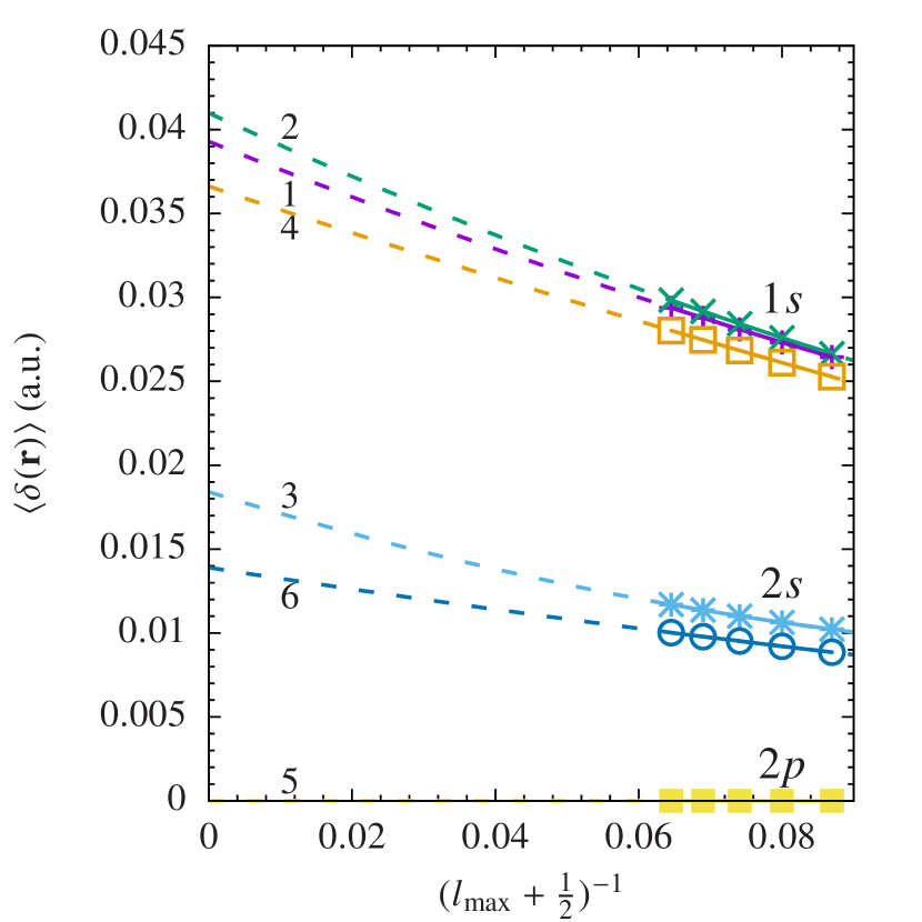
Figure 5: Extrapolation of the expected contact density in $l_{\text{max}}$ for the 6 lowest-energy eigenstates for $J^{\Pi}=0^{+}$, $R_{c}=10$ a.u., and $n_{\text{max}}=15$. Solid lines connect the data points to guide the eye, while the dashed lines show extrapolation to $l_{\rm max}\rightarrow\infty$ using Eq. (25).

Values of the contact density confirm the state identifications made in Sec. II.4.2. States 1, 2, and 4 have contact densities in the range 0.037–0.041, close to the free-Ps value of $1/8\pi\approx 0.0398$ for the $1s$ state. State 5 has an extrapolated contact density of ${\sim}10^{-15}$, confirming that it is a $2p$ state (for which the free-Ps value is zero).

States 3 and 6, which we identify as $2s$ sates, have contact densities 0.018 and 0.014, respectively; the free-Ps value for the $2s$ state is $1/64\pi\approx 0.005$, i.e., about 3 times smaller. The explanation for this difference is that the confining cavity compresses the radial extent of the Ps internal wave function, thereby increasing its density at $\mathbf{r}_{e}=\mathbf{r}_{p}$. This effect has been observed in calculations of radially confined Ps Consolati et al. (2014). The effect of compression on the contact density of Ps in $2s$ states can be estimated from the ratio of the free-Ps mean distance $\langle r\rangle=12$ a.u. to the values obtained in our calculation (Fig. 4). The corresponding density enhancement is proportional to the cube of this ratio, giving $(12/6.9)^{3}/64\pi\approx 0.026$ and $(12/7.9)^{3}/64\pi\approx 0.017$, for states 3 and 6, respectively, that are close to the extrapolated densities in Fig. 5. The same compression effect hardly affects $1s$ states because they are much more compact, and the corresponding electron-positron separation values (for states 1 and 2) are only a little smaller than the free-Ps value of 3 a.u. As noted earlier, the $0^{+}$ states 3 ($1s$) and 4 ($2s$) exhibit some degree of level mixing, which reduces the contact density of the former and increases that of the latter.

Table 1: Calculated energy eigenvalues, center-of-mass momenta, and effective radii for $J^{\Pi}=0^{+}$, $1^{-}$ and $R_{c}=10$ a.u., 12 a.u.

$J^{\Pi}$	$R_{c}$	State no.	$nl[N,L]$	$E(l_{\text{max}},n_{\text{max}})$	$E(\infty,n_{\text{max}})$	$E_{nl[N,L]}$	$K_{nl[N,L]}$	$\rho_{nl[N,L]}$
$0^{+}$	10	1	$1s[1,0]$	$-0.2144498$	$-0.215911$	$-0.216100$	$0.368239$	$1.469$
		2	$1s[2,0]$	$-0.1174946$	$-0.119914$	$-0.120167$	$0.720647$	$1.281$
		3	$2s[1,0]$	$0.02472915$	$0.0241658$	$0.0239796$	$0.588148$	$4.659$
		4	$1s[3,0]$	$0.03396135$	$0.0310792$	$0.0309400$	$1.060075$	$1.109$
		5	$2p[1,1]$	$0.07686479$	$0.0768633$	$0.0768631$	$0.746627$	$3.982$
		6	$2s[2,0]$	$0.1511621$	$0.150550$	$0.150504$	$0.923047$	$3.193$
$0^{+}$	12	1	$1s[1,0]$	$-0.2251509$	$-0.227540$	$-0.227819$	$0.297866$	$1.453$
		2	$1s[2,0]$	$-0.1593054$	$-0.162912$	$-0.163350$	$0.588727$	$1.328$
		3	$1s[3,0]$	$-0.05568137$	$-0.0601980$	$-0.0605930$	$0.870418$	$1.172$
		4	$2s[1,0]$	$-0.01046464$	$-0.0107571$	$-0.0108531$	$0.454519$	$5.088$
		5	$2p[1,1]$	$0.02539311$	$0.0253906$	$0.0253903$	$0.592926$	$4.422$
		6	$2s[2,0]$	$0.07401803$	$0.0721989$	$0.0719415$	$0.733325$	$3.432$
		7	$1s[4,0]$	$0.08558862$	$0.0811920$	$0.0809612$	$1.150585$	$1.078$
$1^{-}$	10	1	$1s[1,1]$	$-0.1787461$	$-0.181426$	$-0.181500$	$0.523450$	$1.416$
		2	$1s[2,1]$	$-0.05370988$	$-0.0571538$	$-0.0573473$	$0.877844$	$1.200$
		3	$2p[1,0]$	$0.004981346$	$0.00497852$	$0.00497844$	$0.519532$	$3.953$
		4	$2s[1,1]$	$0.08365396$	$0.0831681$	$0.0830909$	$0.763128$	$4.112$
		5	$2p[1,2]$	$0.1112176$	$0.111200$	$0.111199$	$0.833544$	$3.086$
		6	$1s[3,1]$	$0.1228439$	$0.118529$	$0.118321$	$1.213789$	$1.016$
		7	$2p[2,0]$	$0.1344290$	$0.134426$	$0.134425$	$0.887525$	$2.921$
$1^{-}$	12	1	$1s[1,1]$	$-0.2004982$	$-0.204725$	$-0.204872$	$0.424867$	$1.424$
		2	$1s[2,1]$	$-0.1152794$	$-0.120225$	$-0.120512$	$0.719689$	$1.266$
		3	$2p[1,0]$	$-0.02131484$	$-0.0213199$	$-0.0213201$	$0.405857$	$4.259$
		4	$1s[3,1]$	$0.006377168$	$6.09126\times 10^{-4}$	$1.97942\times 10^{-4}$	$1.000396$	$1.100$
		5	$2s[1,1]$	$0.02855653$	$0.0278117$	$0.0277551$	$0.600850$	$4.522$
		6	$2p[1,2]$	$0.05077695$	$0.0507504$	$0.0507503$	$0.673054$	$3.437$
		7	$2p[2,0]$	$0.06707912$	$0.0670723$	$0.0670721$	$0.719922$	$3.272$

II.5 Eigenstates with $J\neq 0$

Figures 1–5 showed how the accurate energies, electron-positron separations and contact densities of the 6 lowest-energy $J^{\Pi}=0^{+}$ Ps eigenstates in the cavity of radius $R_{c}$ were obtained. For this symmetry, the electron and positron orbital angular momenta $l_{\nu}$ and $l_{\mu}$ in the expansion (5) are equal, and the dimension of the Hamiltonian matrix in Eq. (7) is $(l_{\text{max}}+1)n_{\text{max}}^{2}$ (3600 in the largest calculation). The ground state of the system describes Ps($1s$) with the orbital angular momentum $L=0$ in the lowest state of the center-of-mass motion, $N=1$. Higher-lying states correspond to excitations of the center-of-mass motion of Ps($1s$) ($N>1$), as well as internal excitations of the Ps atom ($2s$ and $2p$). For $0^{+}$ symmetry, the center-of-mass orbital angular momentum of Ps($2p$) is $L=1$, which is why this state (5 in Fig. 1) lies higher than the lowest $L=0$, $N=1$ state of Ps($2s$) (state 4).

We also calculated the eigenstates for a larger cavity radius $R_{c}=12$ a.u. Increasing $R_{c}$ lowers the energies of all states, and for $J^{\Pi}=0^{+}$ we identify four $1s$ states ($L=0$, $N=1$–4), two $2s$ states ($L=0$, $N=1$, 2), and one $2p$ state ($L=1$, $N=1$); see Table 1. States that lie at higher energies, above the Ps breakup threshold [$E=0$ for free Ps, or above $2\pi^{2}/(2R_{c}^{2})\sim 0.1$ a.u. in the cavity] do not have the form (11) but describe a relatively weakly correlated electron and positron “bouncing” inside the cavity.

To find other states of Ps($2p$) we performed calculations of $J^{\Pi}=1^{-}$ states for both $R_{c}=10$ and 12 a.u. For this symmetry the electron and positron orbital angular momenta are related by $l_{\mu}=l_{\nu}\pm 1$, and the size of the Hamiltonian matrix is $2l_{\text{max}}n_{\text{max}}^{2}$, i.e., about a factor of 2 larger than for $J^{\Pi}=0^{+}$. For computational reasons, it is convenient to define $l_{\text{max}}$ as the maximum angular momentum of one of the particles, e.g., the positron. In this case the electron orbital angular momentum can be as large as $l_{\text{max}}+1$. Limiting its value by 14, we restrict the value of $l_{\text{max}}$ used for extrapolation to the range 10–13. This difference aside, extrapolation of the energy eigenvalues and other quantities for the $1^{-}$ states is performed as described in Sec. II.4. In total, we find 7 eigenstates for $J^{\Pi}=1^{-}$: 3 for Ps($1s$) ($L=0$, $N=1$–3), 3 for Ps($2p$) ($L=0$, $N=1$, 2 and $L=2$, $N=1$), and 1 for Ps($2s$) ($L=1$, $N=1$); see Table 1.

III Results

Table 1 shows the quantum numbers and energy eigenvalues $E_{nl[N,L]}$ of the $J^{\Pi}=0^{+}$ and $1^{-}$ states we found for $R_{c}=10$ and 12 a.u. alongside the corresponding Ps center-of-mass momenta $K_{nl[N,L]}$ and effective Ps radii $\rho_{nl[N,L]}$. As expected, the values of $\rho_{nl[N,L]}$ for the Ps($1s$) states are much smaller than those for Ps in the $2s$ and $2p$ states. The Ps radius for each internal state also displays significant variation with the Ps center-of-mass quantum numbers $N$ and $L$ and with the cavity radius $R_{c}$. It turns out that, to a good approximation, this variation can be analyzed in terms of a single parameter, namely, the Ps center-of-mass momentum $K$.

Figure 6 presents 13 values of the radius of Ps($1s$) states from Table 1, plotted as a function of $K$. The figure shows that, to a very good approximation, the dependence of the Ps radius on its center-of-mass momentum is linear, as described by the fit

$$\rho_{1s}(K)=1.65-0.51K.$$ (26)

When Ps collides with the wall at higher momenta, its effective radius is smaller. This could be expected from a naive picture of Ps as a “soft ball” that gets “squashed” when it hits the hard wall. For higher impact velocities the distortion is stronger, and the Ps center of mass gets closer to the wall. The predicted “static” (i.e., zero-incident-momentum) radius for the $1s$ state is $\rho_{1s}(0)=1.65$ a.u. This value is close to the mean distance between the Ps center of mass and either of its constituent particles, $\frac{1}{2}\langle r\rangle=1.5$ a.u.

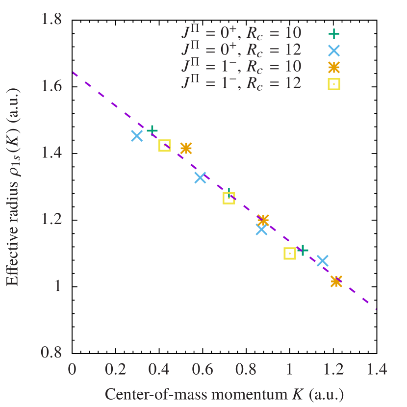
Figure 6: Dependence of the effective Ps($1s$) radius $\rho_{1s}(K)$ on the Ps center-of-mass momentum $K$. The dashed line is the linear fit, Eq. (26).

Figure 7 shows the data for the radius of the $2s$ state. They also suggest a near-linear relationship between the Ps radius and center-of-mass momentum, with two points near $K\approx 0.75$ deviating slightly from it. The larger deviation, observed for the $J^{\Pi}=0^{+}$, $R_{c}=12$ a.u. datum (blue cross), could be, at least in part, due to level mixing between eigenstates 6 and 7, which are separated by a small energy interval (see Table 1). A linear fit of the data gives

$$\rho_{2s}(K)=7.00-4.18K.$$ (27)

The corresponding static radius $\rho_{2s}(0)=7.00$ a.u. is close to the mean radius of free Ps($2s$), $\frac{1}{2}\langle r\rangle=6$ a.u.

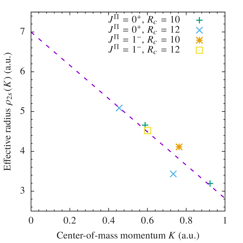
Figure 7: Dependence of the effective Ps($2s$) radius $\rho_{2s}(K)$ on the Ps center-of-mass momentum $K$. The dashed line is the linear fit, Eq. (27).

Finally, Fig. 8 shows the dependence of the radius on the center-of-mass momentum for the Ps($2p$) states. In this case, the 6 data points for the $J^{\Pi}=1^{-}$ states again indicate a linear dependence of $\rho_{2p}$ on $K$, while the points with $J^{\Pi}=0^{+}$ appear as outliers. To understand this behavior, we performed additional sets of calculations for $J^{\Pi}=1^{+}$ and $2^{+}$, with $R_{c}=10$ and 12 a.u. For $J^{\Pi}=1^{+}$ we used $l_{\text{max}}=10$–14 and $n_{\text{max}}=10$–15, while for $J^{\Pi}=2^{+}$ we used $l_{\text{max}}=9$–13 and $n_{\text{max}}=8$–13, due to computational restrictions. For both values of $R_{c}$ we found one Ps($2p$) state with $N=1$ and $L=1$ for each symmetry. Table 2 shows the data for these states.

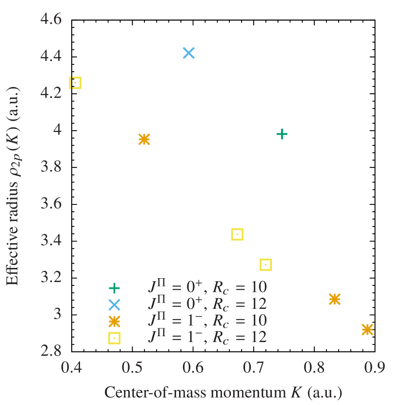
Figure 8: Dependence of the effective Ps($2p$) radius $\rho_{2p}(K)$ on the Ps center-of-mass momentum $K$.

Table 2: Calculated energy eigenvalues, center-of-mass momenta, and effective radii for $J^{\Pi}=1^{+}$, $2^{+}$ and $R_{c}=10$ and 12 a.u. Only the Ps($2p$) states are shown.

$J^{\Pi}$	$R_{c}$	State no.	$[N,L]$	$E_{2p[N,L]}$	$K_{2p[N,L]}$	$\rho_{2p[N,L]}$
$1^{+}$	10	1	$[1,1]$	$0.0477391$	$0.664045$	$3.233$
$1^{+}$	12	1	$[1,1]$	$0.00718021$	$0.527940$	$3.489$
$2^{+}$	10	3	$[1,1]$	$0.0576334$	$0.693205$	$3.518$
$2^{+}$	12	3	$[1,1]$	$0.0134862$	$0.551312$	$3.850$

Figure 9 shows the dependence of the radius on the momentum for the Ps($2p$) states, using the data from all of the calculations performed. As noted above, the negative-parity $J^{\Pi}=1^{-}$ data that describe the states of Ps($2p$) with the center-of-mass angular momentum $L=0$ or 2 display a clear linear trend. In contrast, the three positive-parity states with $J^{\Pi}=0^{+}$, $1^{+}$, and $2^{+}$ (for a given $R_{c}$) do not follow the trend and suggest $J$-dependent values of the Ps radius. These states correspond to three possible ways of coupling the Ps($2p$) internal angular momentum $l=1$ and its center-of-mass angular momentum $L=1$. Since neither Ps($2p$) nor its center-of-mass wave function for $L=1$ [cf. Eq. (11)] is spherically symmetric, it is not surprising that the distance of closest approach to the wall (i.e., the Ps radius) depends on the asymmetry of the center-of-mass motion through $J$. A simple perturbative estimate of the $J$ splitting of these states is provided in Appendix B.

To define a spherically averaged collisional radius of Ps($2p$) we take a weighted average of these data $(K_{J},\rho_{2p[1,1]J})$ with weights $2J+1$ for each $R_{c}$. The corresponding values are shown by diamonds in Fig. 9. They lie close to the $J^{\Pi}=2^{+}$ date points (see Appendix B for an analytical explanation), and agree very well with the momentum dependence predicted by the $J^{\Pi}=1^{-}$ data. Using these together gives the linear fit

$$\rho_{2p}(K)=5.35-2.77K.$$ (28)

The static radius for the $2p$ state $\rho_{2p}(0)=5.35$ a.u. is again close to the mean radius of free Ps($2p$), i.e., $\frac{1}{2}\langle r\rangle=5$ a.u.

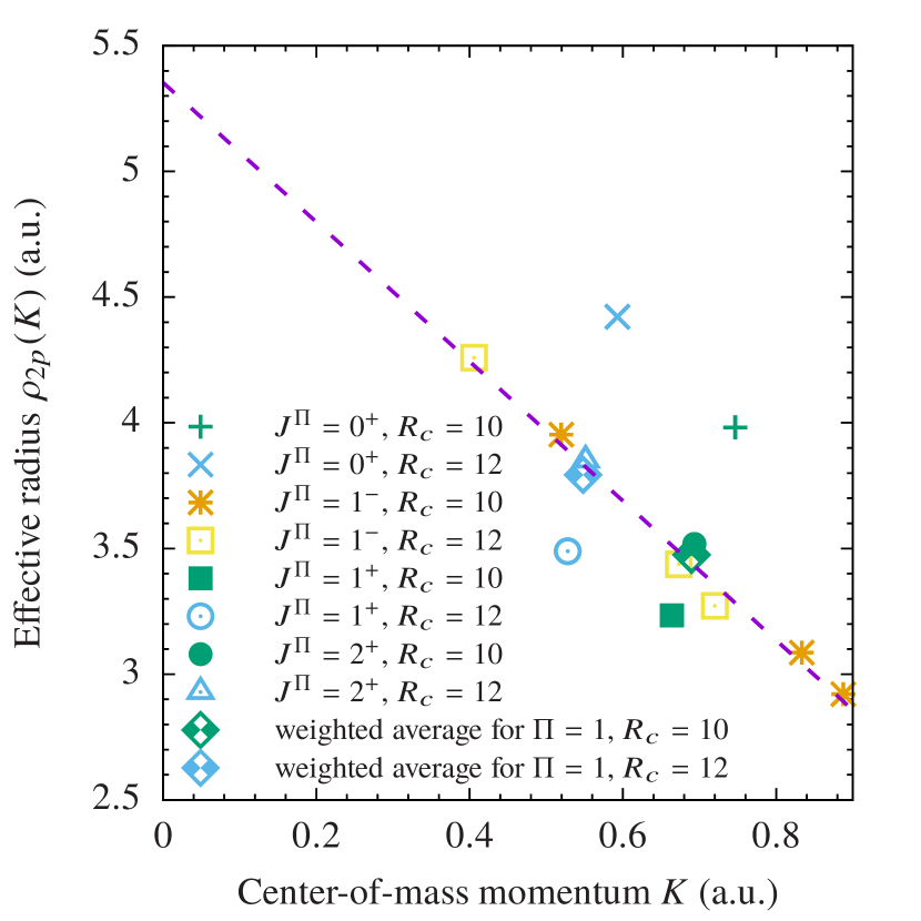
Figure 9: Dependence of the effective Ps($2p$) radius $\rho_{2p}(K)$ on the Ps center-of-mass momentum $K$, including data for $J^{\Pi}=1^{+}$ and $2^{+}$ states. The dashed line is the linear fit, Eq. (28).

Regarding $J^{\Pi}=1^{-}$ data, the Ps($2p$) radii in the states with $L=0$ (two for each of $R_{c}$) are naturally spherically averaged. The $J^{\Pi}=1^{-}$ states with $L=2$ are parts of the $J$-dependent manifold ($J=1$, 2, and 3). Here it appears that the $J=1$ state here is close to the $J$-averaged value (see Appendix B), so that all $J^{\Pi}=1^{-}$ data follow the same linear momentum dependence.

III.1 Estimate of the cavity shift of Lyman-$\alpha$ transition

Measuments of the Ps Lyman-$\alpha$ transition in porous silica revealed a blue shift of the transition energy $\Delta E=1.26\pm 0.06$ meV Cassidy et al. (2011). The pore size in this material is estimated to be $a\sim 5~{}\text{nm}$ Crivelli et al. (2010). Assuming spherical pores for simplicty, we find their radius $R_{c}\sim 50$ a.u. The Ps center-of-mass momentum in the lowest energy state in such pores is $K\simeq\pi/R_{c}\sim 0.06$ a.u. For such a small momentum one can use static values of the Ps radius in $1s$ and $2p$ states (see Figs. 6 and 9). Considering $S$-wave Ps ($L=0$), we estimate the cavity shift of the Lyman-$\alpha$ transition energy from Eq. (14),

$$\Delta E\simeq\frac{\pi^{2}}{2R_{c}^{3}}(\rho_{2p}-\rho_{1s}).$$ (29)

For static radii $\rho_{1s}=1.65$ a.u. and $\rho_{2p}=5.35$ a.u., and $R_{c}=50$ a.u., we obtain $\Delta E=4$ meV. This value is close to the naive estimate using mean Ps radii Cassidy et al. (2011) and is significantly larger than the experimental value.

It appears from the measured $\Delta E$ that the radius of Ps($2p$) is only slightly greater than that of Ps($1s$). This effect is likely due to the nature of Ps interaction with the wall in a real material. The Ps($2p$) state is degenerate with Ps($2s$), and their linear combination (a hydrogenic eigenstate in parabolic coordinates Landau and Lifshitz (1965)) can possess a permanent dipole moment. Such a state can have a stronger, more attractive interaction with the cavity wall than the ground state Ps($1s$). This interaction will result in an additional phase shift of the Ps center-of-mass wave function reflected by the wall. The scattering phase shift $\delta_{nl}(K)$ is related to the Ps radius $\rho_{nl}(K)$ by $\delta_{nl}(K)=-K\rho_{nl}(K)$ [cf. Eq. (13)], with the static radius $\rho_{nl}(0)$ playing the role of the scattering length. It is known that the van der Waals interaction between the ground-state Ps and noble-gas atoms can significantly reduce the magnitude of the scatetring length Mitroy and Ivanov (2001); Mitroy and Bromley (2003); Fabrikant and Gribakin (2014); Swann and Gribakin (2017). It can be expected that a similar dispersive interaction between excited-state Ps and the cavity wall can reduce the effective radius of Ps($2p$) by more than that of Ps($1s$), to produce the difference $\rho_{2p}-\rho_{1s}\approx 1$ a.u. compatible with experiment.

IV Conclusions

A $B$-spline basis was employed to obtain single-particle electron and positron states within an otherwise empty spherical cavity. These states were used to construct the two-particle states of positronium, including only finitely many partial waves and radial states in the expansion. Diagonalization of the Hamiltonian matrix allowed us to determine the energy and expectation values of the electron-positron separation and contact density for each state. Extrapolation of the energy with respect to the maximum orbital angular momentum $l_{\text{max}}$ and the number of radial states $n_{\text{max}}$ included for each partial wave was carried out. The electron-positron separation and contact density values were also extrapolated with respect to the number of partial waves included and used to determine the nature (i.e., the quantum numbers) of each positronium state. From the extrapolated energies, the effective collisional radius of the positronium atom was determined for each state.

We have found that the radius of the Ps atom in the ground state has a linear dependence on the Ps center-of-mass momentum, Eq. (26), the radius being smaller for higher impact momenta. The radius of Ps($2s$) also displays a linear momentum dependence, Eq. (27). The static (i.e., zero-momentum) collisional radii of the $1s$ and $2s$ states are 1.65 and 7 a.u., respectively. Determining the effective radius of Ps in $2p$ state is more complex due to its asymmetry. Spherically averaged values of the collisional radius are obtained directly for Ps $S$-wave states in the cavity, with Ps $D$-wave states giving similar radii. However, determining the corresponding values for the Ps $P$-wave states required averaging over the total angular momentum of the Ps states in the cavity. (See Appendix B for a quantitative explanation for the $J$ dependence of the $2p[1,1]$ and $2p[1,2]$ energy levels.) After this, all data points were found to follow the linear dependence on the Ps momentum, giving the static radius of 5.35 a.u. In all three cases, the static values of the effective Ps radius are close to the expectation value of the radius of free Ps, i.e., a half of the mean electron-positron separation.

While the linear fits obtained here for the dependence of the effective Ps radius on the center-of-mass momentum are clearly very good, particularly for the $1s$ state, it must be noted that there is a certain amount of scatter around the lines. This phenomenon may be due to numerical errors in the two-particle-state calculations or in the extrapolation of the energy eigenvalues (or both). The main issue here is the slow convergence of the single-center expansion for states that describe the compact Ps atom away from the origin. This issue also prevented us from perfoming calculations for larger-sized cavities, which would provide effective Ps radii for lower center-of-mass momenta. A possible means to reduce the scatter in the data and tackle large cavities could be to include more partial waves and radial states per partial wave in the CI expansion. However, with the Hamiltonian matrix dimensions increasing as $l_{\text{max}}n_{\text{max}}^{2}$, this quickly becomes computationally expensive. An alternative would be to use a variational approach with explicitly correlated two-particle wave functions.

Although we have only considered the $1s$, $2s$, and $2p$ states in the present work, it is possible to use the method to investigate the effective radii of higher excited states, e.g., the $3s$, $3p$ and $3d$ states. However, this would require calculations with much larger cavities that can fit the $n=3$ Ps states without significantly squeezing them.

It was noted earlier that confinement can cause a Ps atom to “shrink” from its size in vacuo. This manifests in the form of a reduced electron-positron separation and increased contact density; these effects were observed for the $2s$ and $2p$ states. While this is true in an idealized hard-wall cavity, in physical cavities (e.g., in a polymer) there is a second, competing effect. Polarization of the Ps atom by the surrounding matter may actually lead to a swollen Ps atom, which causes the contact density to be reduced from its value in vacuo Dupasquier (1983); McMullen and Scott (1983). Experimentally, it has generally been found that the net result of these two effects is that the contact density is reduced from its in-vacuo value, although increased values are not necessarily impossible McMullen and Scott (1983); Brandt et al. (1960). It may be possible to determine more physical effective Ps radii by using realistic electron- and positron-wall potentials in place of the hard wall we have used here. Such developement of the approach adopted in the present work should yield much more reliable data for the distorted Ps states than crude model calculations Marlotti Tanzi et al. (2016).

The technique outlined in this paper is eminently suitable for implementing a bound-state approach to low-energy Ps-atom scattering. By calculating single-particle electron and positron states in the field of an atom at the center of the cavity (rather than the empty cavity) and constructing two-particle Ps wave functions from these, a shifted set of energy levels may be found. From these, the Ps-atom scattering phase shifts can be determined [cf. Eq. (1)] using the now known collisional radius of Ps. We have carried out several preliminary calculations in this area for elastic Ps($1s$)-Ar scattering at the static (Hartree-Fock) level and found a scattering length of 2.85 a.u., in perfect agreement with an earlier fixed-core stochastic variational method calculation in the static approximation by Mitroy and Ivanov Mitroy and Ivanov (2001). This provides evidence that the linear fits presented here account for the finite size of the Ps atom in scattering calculations very accurately. In our calculations we have also observed fragmented Ps states at higher energies (this manifests as a larger-than-usual electron-positron separation). These have been ignored in the present work, but it may be possible to use them to obtain information about inelastic scattering using this method.

It is hoped that the results presented here will be of use in future studies of both confined positronium and positronium-atom scattering.

Appendix A Working expressions for the Hamiltonian matrix and expectation values

Written in terms of the angular and radial parts of the electron and positron basis states, the Ps wave function is

$$\Psi_{J\Pi}(\mathbf{r}_{e},\mathbf{r}_{p}) =\frac{1}{r_{e}r_{p}}\sum_{\begin{subarray}{c}\mu,\nu\\ m_{\mu},m_{\nu}\end{subarray}}C^{(J)}_{\mu\nu}P_{\mu}(r_{e})P_{\nu}(r_{p})$$

$$\quad{}\times C^{JM}_{l_{\mu}m_{\mu}l_{\nu}m_{\nu}}Y_{l_{\mu}m_{\mu}}(\Omega_{e})Y_{l_{\nu}m_{\nu}}(\Omega_{p}),$$ (30)

where $C^{JM}_{l_{\mu}m_{\mu}l_{\nu}m_{\nu}}$ is the Clebsch-Gordan coefficient, and the indices $\mu$ and $\nu$ enumerate the radial electron and positron basis states with various orbital angular momenta, $\mu\equiv\varepsilon_{\mu}l_{\mu}$ and $\nu\equiv\varepsilon_{\nu}l_{\nu}$. Besides the selection rules due to the Clebsch-Gordan coefficient, the summation is restricted by parity, $(-1)^{l_{\mu}+l_{\nu}}=\Pi$, where $\Pi=1$ $(-1)$ for the even (odd) states.

Integration over the angular variables in the Coulomb matrix elements is performed analytically Varshalovich et al. (1988), and the Hamiltonian matrix elements for the Ps states with the total angular momentum $J$ are given by

$$H^{(J)}_{\mu^{\prime}\nu^{\prime},\mu\nu} =(\varepsilon_{\mu}+\varepsilon_{\nu})\delta_{\mu\mu^{\prime}}\delta_{\nu\nu^{\prime}}+V^{(J)}_{\mu^{\prime}\nu^{\prime},\mu\nu},$$ (31)

where

$$V^{(J)}_{\mu^{\prime}\nu^{\prime},\mu\nu}=\sum_{l}(-1)^{J+l}\begin{Bmatrix}J&l_{\mu^{\prime}}&l_{\nu^{\prime}}\\ l&l_{\nu}&l_{\mu}\end{Bmatrix}\langle\nu^{\prime}\mu^{\prime}\|V_{l}\|\mu\nu\rangle,$$ (32)

and the reduced Coulomb matrix element is

$$\langle\nu^{\prime}\mu^{\prime}\|V_{l}\|\mu\nu\rangle =\sqrt{[l_{\nu^{\prime}}][l_{\mu^{\prime}}][l_{\mu}][l_{\nu}]}\begin{pmatrix}l_{\mu^{\prime}}&l&l_{\mu}\\ 0&0&0\end{pmatrix}\begin{pmatrix}l_{\nu^{\prime}}&l&l_{\nu}\\ 0&0&0\end{pmatrix}$$

$$\quad{}\times\int_{0}^{R_{c}}\!\!\int_{0}^{R_{c}}P_{\nu^{\prime}}(r_{p})P_{\mu^{\prime}}(r_{e})\frac{r_{<}^{l}}{r_{>}^{l+1}}$$

$$\quad{}\times P_{\mu}(r_{e})P_{\nu}(r_{p})\,dr_{e}\,dr_{p},$$ (33)

with $[l]\equiv 2l+1$, $r_{<}=\min(r_{e},r_{p})$, and $r_{>}=\max(r_{e},r_{p})$.

The expectation value of the electron-positron separation $r_{ep}=\lvert\mathbf{r}_{e}-\mathbf{r}_{p}\rvert$ for an eigenstate with eigenvector $C^{(J)}_{\mu\nu}$ is found as

$$\langle r_{ep}\rangle=\sum_{\begin{subarray}{c}\mu^{\prime},\nu^{\prime}\\ \mu,\nu,l\end{subarray}}C^{(J)}_{\mu^{\prime}\nu^{\prime}}C^{(J)}_{\mu\nu}(-1)^{J+l}\begin{Bmatrix}J&l_{\mu^{\prime}}&l_{\nu^{\prime}}\\ l&l_{\nu}&l_{\mu}\end{Bmatrix}\langle\nu^{\prime}\mu^{\prime}\|S_{l}\|\mu\nu\rangle,$$ (34)

where

$$\langle\nu^{\prime}\mu^{\prime}\|S_{l}\|\mu\nu\rangle =\sqrt{[l_{\nu^{\prime}}][l_{\mu^{\prime}}][l_{\mu}][l_{\nu}]}\begin{pmatrix}l_{\mu^{\prime}}&l&l_{\mu}\\ 0&0&0\end{pmatrix}\begin{pmatrix}l_{\nu^{\prime}}&l&l_{\nu}\\ 0&0&0\end{pmatrix}$$

$$\quad{}\times\int_{0}^{R_{c}}\!\!\int_{0}^{R_{c}}P_{\nu^{\prime}}(r_{p})P_{\mu^{\prime}}(r_{e})\frac{r_{<}^{l}}{r_{>}^{l+1}}$$

$$\quad{}\times\mathopen{}\mathclose{{}\left(\frac{r_{<}^{2}}{2l+3}-\frac{r_{>}^{2}}{2l-1}}\right)P_{\mu}(r_{e})P_{\nu}(r_{p})\,dr_{e}\,dr_{p}.$$ (35)

Similarly, the expectation value of the electron-positron contact density $\delta_{ep}=\delta(\mathbf{r}_{e}-\mathbf{r}_{p})$ is

$$\langle\delta_{ep}\rangle=\sum_{\begin{subarray}{c}\mu^{\prime},\nu^{\prime}\\ \mu,\nu,l\end{subarray}}C^{(J)}_{\mu^{\prime}\nu^{\prime}}C^{(J)}_{\mu\nu}(-1)^{J+l}\begin{Bmatrix}J&l_{\mu^{\prime}}&l_{\nu^{\prime}}\\ l&l_{\nu}&l_{\mu}\end{Bmatrix}\langle\nu^{\prime}\mu^{\prime}\|\delta_{l}\|\mu\nu\rangle,$$ (36)

where

$$\langle\nu^{\prime}\mu^{\prime}\|\delta_{l}\|\mu\nu\rangle =\sqrt{[l_{\nu^{\prime}}][l_{\mu^{\prime}}][l_{\mu}][l_{\nu}]}\begin{pmatrix}l_{\mu^{\prime}}&l&l_{\mu}\\ 0&0&0\end{pmatrix}\begin{pmatrix}l_{\nu^{\prime}}&l&l_{\nu}\\ 0&0&0\end{pmatrix}$$

$$\quad{}\times\frac{[l]}{4\pi}\int_{0}^{R_{c}}P_{\nu^{\prime}}(r)P_{\mu^{\prime}}(r)P_{\mu}(r)P_{\nu}(r)\frac{dr}{r^{2}}.$$ (37)

Appendix B Splitting of Ps $nl[N,L]$ states due to interaction with the cavity wall

The angular part of the Ps wave function in the cavity, Eq. (11), is

$$\Theta_{lL}^{(J)}(\Omega_{\mathbf{r}},\Omega_{\mathbf{R}})=\sum_{m,M_{L}}C_{lmLM_{L}}^{JM}Y_{lm}(\Omega_{\mathbf{r}})Y_{LM_{L}}(\Omega_{\mathbf{R}}).$$ (38)

The electron and positron repulsion from the wall is strongest when the vectors $\mathbf{r}$ and $\mathbf{R}$ are parallel or antiparallel. In the simplest approximation, we can take the corresponding perturbation as being proportional to $\cos^{2}\theta$, where $\theta$ is the angle between $\mathbf{r}$ and $\mathbf{R}$. Shifting this by a constant to make the spherical average of the perturbation zero, we write it as

$$\delta V(\Omega_{\mathbf{r}},\Omega_{\mathbf{R}})=\alpha P_{2}(\cos\theta),$$ (39)

where $\alpha$ is a constant that can depend on the quantum numbers $n$ and $N$ and on the cavity radius $R_{c}$, and $P_{2}$ is the second Legendre polynomial. The corresponding energy shift is

$$\Delta E_{J}^{\text{(pert)}}=\alpha\iint\mathopen{}\mathclose{{}\left\lvert\Theta_{lL}^{(J)}(\Omega_{\mathbf{r}},\Omega_{\mathbf{R}})}\right\rvert^{2}P_{2}(\cos\theta)\,d\Omega_{\mathbf{r}}\,d\Omega_{\mathbf{R}},$$ (40)

by first-order perturbation theory. Intergating over the angles, one obtains Varshalovich et al. (1988)

$$\Delta E_{J}^{\text{(pert)}} =\alpha(2l+1)(2L+1)\begin{pmatrix}l&2&l\\ 0&0&0\end{pmatrix}\begin{pmatrix}L&2&L\\ 0&0&0\end{pmatrix}$$

$$\quad{}\times(-1)^{J}\begin{Bmatrix}L&l&J\\ l&L&2\end{Bmatrix}$$

$$=\alpha(2l+1)(2L+1)\begin{pmatrix}l&2&l\\ 0&0&0\end{pmatrix}\begin{pmatrix}L&2&L\\ 0&0&0\end{pmatrix}$$

$$\quad{}\times(-1)^{l+L}\sqrt{\frac{(2L-2)!\,(2l-2)!}{(2L+3)!\,(2l+3)!}}\,\mathopen{}\mathclose{{}\left(6X^{2}+6X-8Y}\right),$$ (41)

where $X=J(J+1)-l(l+1)-L(L+1)$ and $Y=l(l+1)L(L+1)$.

It is easy to check that the average energy shift is zero, i.e.,

$$\sum_{J}(2J+1)\Delta E_{J}^{\text{(pert)}}=0,$$ (42)

as it should be for a perturbation with a zero spherical average, $\langle\delta V\rangle=0$.

For Ps states $2p[1,1]$ and $2p[1,2]$ the possible values of $J$ are 0, 1, 2 and 1, 2, 3 respectively. In each case, let $E_{J}$ denote the calculated energy eigenvalues of the $J$ manifold, with the average energy

$$\langle E_{J}\rangle=\frac{\sum_{J}(2J+1)E_{J}}{\sum_{J}(2J+1)}.$$ (43)

To compare the numerical energy shifts $\Delta E_{J}\equiv E_{J}-\langle E_{J}\rangle$ with $\Delta E_{J}^{\text{(pert)}}$, we choose $\alpha$ to reproduce the calculated mean-squared shift, viz.,

$$\sum_{J}(2J+1)\mathopen{}\mathclose{{}\left[\Delta E_{J}^{\text{(pert)}}}\right]^{2}=\sum_{J}(2J+1)\mathopen{}\mathclose{{}\left[\Delta E_{J}}\right]^{2}.$$ (44)

Table 3 shows the energy eigenvalues, $J$-averaged energies, numerical and perturbative energy shifts $\Delta E_{J}$ and $\Delta E_{J}^{\text{(pert)}}$, as well as the values of $\alpha$, for Ps($2p$) states with $L=1$ and $L=2$, for $R_{c}=10$ and 12 a.u.

Table 3: Comparison of the energy shifts $\Delta E_{J}$ obtained from the numerical eigenvalues $E_{J}$ with the perturbative estimates $\Delta E_{J}^{\text{(pert)}}$, Eq. (41), for Ps($2p$) states with $N=1$ and $L=1,\,2$, for cavity radii $R_{c}=10$ and 12 a.u.

$nl[N,L]$	$R_{c}$	$J^{\Pi}$	$E_{J}$	$\langle E_{J}\rangle$	$\Delta E_{J}$	$\Delta E_{J}^{\text{(pert)}}/\alpha$	$\alpha$	$\Delta E_{J}^{\text{(pert)}}$
$2p[1,1]$	10	$0^{+}$	$0.0768631$		$0.0203912$	$2/5$		$0.019022$
		$1^{+}$	$0.0477391$	$0.0564719$	$-0.0087328$	$-1/5$	$0.047556$	$-0.009511$
		$2^{+}$	$0.0576334$		$0.0011615$	$1/25$		$0.001902$
	12	$0^{+}$	$0.0253903$		$0.0126834$	$2/5$		$0.011915$
		$1^{+}$	$0.00718021$	$0.0127069$	$-0.0055267$	$-1/5$	$0.029787$	$-0.005957$
		$2^{+}$	$0.0134862$		$0.0007793$	$1/25$		$0.001191$
$2p[1,2]$	10	$1^{-}$	$0.111199$		$-0.000037$	$1/5$		$0.008045$
		$2^{-}$	$0.103201$	$0.111236$	$-0.008035$	$-1/5$	$0.040224$	$-0.008045$
		$3^{-}$	$0.116992$		$0.005756$	$2/35$		$0.002299$
	12	$1^{-}$	$0.0507503$		$0.0008605$	$1/5$		$0.005357$
		$2^{-}$	$0.0443476$	$0.0498898$	$-0.0055422$	$-1/5$	$0.026787$	$-0.005357$
		$3^{-}$	$0.0534797$		$0.0035899$	$2/35$		$0.001531$

To complete the multiplet for $L=2$, calculations for $J^{\Pi}=2^{-}$ and $3^{-}$ were carried out using $l_{\text{max}}=9$–13 and $n_{\text{max}}=8$–13. For a given $R_{c}$ the values of $\alpha$ for $L=1$ and 2 states are similar. On the other hand, when $R_{c}$ increases from 10 to 12 a.u., the values of $\alpha$ decrease as $1/R_{c}^{q}$ with $q\sim 2.5$. This is close to the expected $1/R_{c}^{3}$ dependence of the energy shifts with the cavity radius Green and Gribakin (2011).

Figures 10 and 11 compare the values of $\Delta E_{J}$ with their perturbative estimates $\Delta E_{J}^{\text{(pert)}}$ for $R_{c}=10$ a.u. and 12 a.u. respectively.

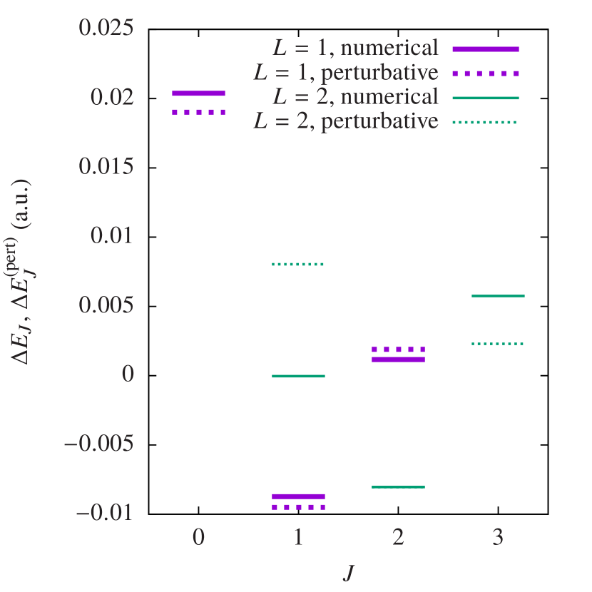
Figure 10: Values of $\Delta E_{J}$ and $\Delta E_{J}^{\text{(pert)}}$ for the $2p[1,1]$ and $2p[1,2]$ states in a cavity of radius $R_{c}=10$ a.u.

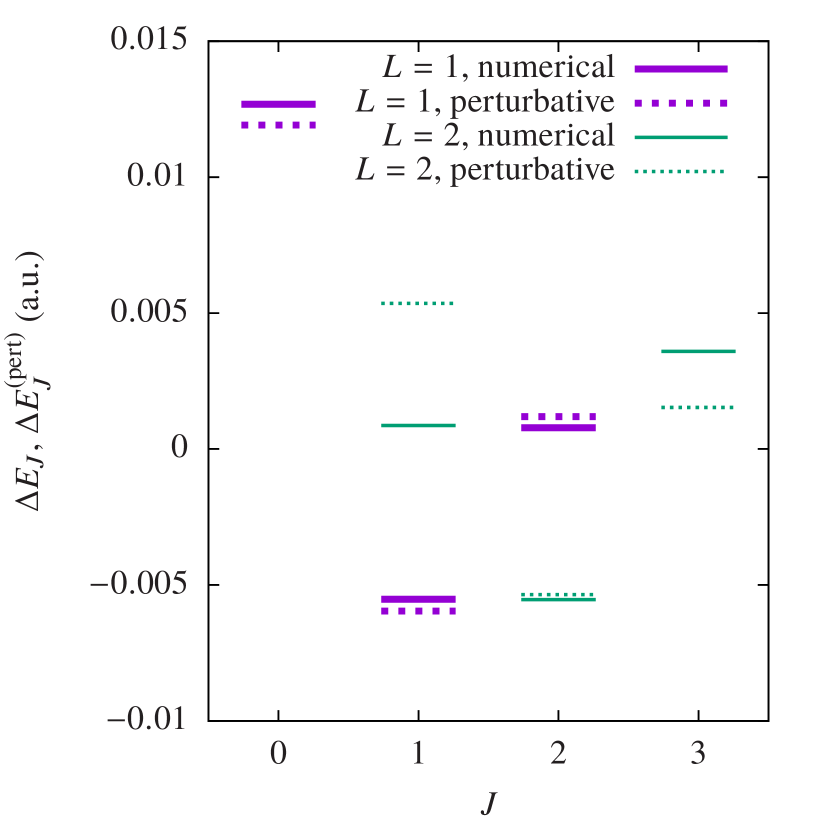
Figure 11: Values of $\Delta E_{J}$ and $\Delta E_{J}^{\text{(pert)}}$ for the $2p[1,1]$ and $2p[1,2]$ states in a cavity of radius $R_{c}=12$ a.u.

For $L=1$ the perturbative estimates of the energy shifts are in excellent agreement with their numerical counterparts. Note that the small shift of the $J^{\Pi}=2^{+}$ level is explained by the small magnitude of the corresponding $6j$ symbol in Eq. (41). For $L=2$ states, the perturbative estimate reproduces the overall $J$ dependence of the calculated energy shift, with the $J=2$ state being the lowest of the three. However, the relative positions of the $J^{\Pi}=1$ and 3 states are reversed. This is probably due to higher-order corrections or level mixing not described by Eq. (39). Note that the numerical shift is smallest for the $J=1$ state, which justifies its use in determining the fit (28).

References

- Cassidy et al. (2011) D. B. Cassidy, M. W. J. Bromley, L. C. Cota, T. H. Hisakado, H. W. K. Tom, and A. P. Mills, Jr., Phys. Rev. Lett. 106, 023401 (2011).
- Green and Gribakin (2011) D. G. Green and G. F. Gribakin, Phys. Rev. Lett. 106, 209301 (2011), (in this paper the Ps radius is estimated as the mean electron-positron separation , while it seems better to use ).
- Tao (1972) S. J. Tao, J. Chem. Phys. 56, 5499 (1972).
- Eldrup et al. (1981) M. Eldrup, D. Lightbody, and J. N. Sherwood, Chem. Phys. 63, 51 (1981).
- Schrader and Jean (1988) D. M. Schrader and Y. C. Jean, eds., Positron and Positronium Chemistry, Studies in Physical and Theoretical Chemistry, Vol. 57 (Elsevier, New York, 1988).
- Gidley et al. (1999) D. W. Gidley, W. E. Frieze, T. L. Dull, A. F. Yee, E. T. Ryan, and H.-M. Ho, Phys. Rev. B 60, R5157 (1999).
- Goworek et al. (2002) T. Goworek, B. Jasińska, J. Wawryszczuk, R. Zaleski, and T. Suzuki, Chem. Phys. 280, 295 (2002).
- Wada and Hyodo (2013) K. Wada and T. Hyodo, J. Phys. Conf. Ser. 443, 012003 (2013).
- Cassidy and Mills, Jr. (2011) D. B. Cassidy and A. P. Mills, Jr., Phys. Rev. Lett. 107, 213401 (2011).
- Cassidy and Mills, Jr. (2007a) D. B. Cassidy and A. P. Mills, Jr., Nature 449, 195 (2007a).
- Cassidy et al. (2012) D. B. Cassidy, T. H. Hisakado, H. W. K. Tom, and A. P. Mills, Jr., Phys. Rev. Lett. 108, 133402 (2012).
- Cassidy and Mills, Jr. (2007b) D. B. Cassidy and A. P. Mills, Jr., Physica Status Solidi (c) 4, 3419 (2007b).
- Michels et al. (1937) A. Michels, J. de Boer, and A. Bijl, Physica 4, 981 (1937).
- Sommerfeld and Welker (1938) A. Sommerfeld and H. Welker, Ann. Phys. (Leipzig) 424, 56 (1938).
- Jaskólski (1996) W. Jaskólski, Phys. Rep. 271, 1 (1996).
- Buchachenko (2001) A. L. Buchachenko, J. Chem. Phys. B 105, 5839 (2001).
- Connerade and Kengkan (2003) J.-P. Connerade and P. Kengkan, in Proc. Idea-Finding Symp. (Frankfurt Institute for Advanced Studies, 2003) pp. 35–46.
- Connerade and Kengkan (2005) J.-P. Connerade and P. Kengkan, in Electron Scattering, Physics of Atoms and Molecules, edited by C. T. Whelan and N. J. Mason (Springer, New York, 2005) pp. 1–11.
- Sabin and Brandas (2009a) J. R. Sabin and E. J. Brandas, eds., Theory of Confined Quantum Systems—Part One, Advances in Quantum Chemistry, Vol. 57 (Academic Press, New York, 2009).
- Sabin and Brandas (2009b) J. R. Sabin and E. J. Brandas, eds., Theory of Confined Quantum Systems—Part Two, Advances in Quantum Chemistry, Vol. 58 (Academic Press, New York, 2009).
- Lawrence et al. (1981) J. M. Lawrence, P. S. Riseborough, and R. D. Parks, Rep. Prog. Phys. 44, 1 (1981).
- Connerade and Semaoune (2000) J. P. Connerade and R. Semaoune, J. Phys. B 33, 3467 (2000).
- Bethune et al. (1993) D. D. Bethune, R. D. Johnson, J. R. Salem, M. S. de Vries, and C. S. Yannoni, Nature 366, 123 (1993).
- Shinohara (2000) H. Shinohara, Rep. Prog. Phys. 63, 843 (2000).
- Komatsu et al. (2005) K. Komatsu, M. Murata, and Y. Murata, Science 307, 238 (2005).
- Marlotti Tanzi et al. (2016) G. Marlotti Tanzi, F. Castelli, and G. Consolati, Phys. Rev. Lett. 116, 033401 (2016).
- Bernauer et al. (2010) J. C. Bernauer, P. Achenbach, C. Ayerbe Gayoso, R. Böhm, D. Bosnar, L. Debenjak, M. O. Distler, L. Doria, A. Esser, H. Fonvieille, J. M. Friedrich, J. Friedrich, M. Gómez Rodríguez de la Paz, M. Makek, H. Merkel, D. G. Middleton, U. Müller, L. Nungesser, J. Pochodzalla, M. Potokar, S. Sánchez Majos, B. S. Schlimme, S. Širca, T. Walcher, and M. Weinriefer (A1 Collaboration), Phys. Rev. Lett. 105, 242001 (2010).
- Antognini et al. (2013) A. Antognini, F. Nez, K. Schuhmann, F. D. Amaro, F. Biraben, J. M. R. Cardoso, D. S. Covita, A. Dax, S. Dhawan, M. Diepold, L. M. P. Fernandes, A. Giesen, A. L. Gouvea, T. Graf, T. W. Hänsch, P. Indelicato, L. Julien, C.-Y. Kao, P. Knowles, F. Kottmann, E.-O. Le Bigot, Y.-W. Liu, J. A. M. Lopes, L. Ludhova, C. M. B. Monteiro, F. Mulhauser, T. Nebel, P. Rabinowitz, J. M. F. dos Santos, L. A. Schaller, C. Schwob, D. Taqqu, J. F. C. A. Veloso, J. Vogelsang, and R. Pohl, Science 339, 417 (2013).
- Landau and Lifshitz (1965) L. D. Landau and E. M. Lifshitz, Quantum Mechanics: Non-Relativistic Theory, 2nd ed. (Pergamon Press, Oxford, 1965).
- Swann and Gribakin (2017) A. R. Swann and G. F. Gribakin, “Positronium scattering by noble-gas atoms using a spherical cavity,” (2017), (unpublished).
- Burke (1977) P. G. Burke, Potential Scattering in Atomic Physics (Springer, New York, 1977).
- de Boor (2001) C. de Boor, A Practical Guide to Splines, revised ed., Applied Mathematical Sciences, Vol. 27 (Springer, New York, 2001).
- Note (1) We use an x86_64 Beowulf cluster.
- Kutzelnigg and Morgan (1992) W. Kutzelnigg and J. D. Morgan, J. Chem. Phys. 96, 4484 (1992).
- Gribakin and Ludlow (2002) G. F. Gribakin and J. Ludlow, J. Phys. B 35, 339 (2002).
- Bray and Stelbovics (1993) I. Bray and A. T. Stelbovics, Phys. Rev. A 48, 4787 (1993).
- Gribakin and Ludlow (2004) G. F. Gribakin and J. Ludlow, Phys. Rev. A 70, 032720 (2004).
- Mitroy and Bromley (2006) J. Mitroy and M. W. J. Bromley, Phys. Rev. A 73, 052712 (2006).
- Zammit et al. (2013) M. C. Zammit, D. V. Fursa, and I. Bray, Phys. Rev. A 87, 020701 (2013).
- Green and Gribakin (2013) D. G. Green and G. F. Gribakin, Phys. Rev. A 88, 032708 (2013).
- Green et al. (2014) D. G. Green, J. A. Ludlow, and G. F. Gribakin, Phys. Rev. A 90, 032712 (2014).
- Consolati et al. (2014) G. Consolati, F. Quasso, and D. Trezzi, PLoS One 9, e109937 (2014).
- Crivelli et al. (2010) P. Crivelli, U. Gendotti, A. Rubbia, L. Liszkay, P. Perez, and C. Corbel, Phys. Rev. A 81, 052703 (2010).
- Mitroy and Ivanov (2001) J. Mitroy and I. A. Ivanov, Phys. Rev. A 65, 012509 (2001).
- Mitroy and Bromley (2003) J. Mitroy and M. W. J. Bromley, Phys. Rev. A 67, 034502 (2003).
- Fabrikant and Gribakin (2014) I. I. Fabrikant and G. F. Gribakin, Phys. Rev. A 90, 052717 (2014).
- Dupasquier (1983) A. Dupasquier, in Positron Solid State Physics, edited by W. Brandt and A. Dupasquier (New Holland, Amsterdam, 1983) pp. 510–64.
- McMullen and Scott (1983) T. McMullen and M. T. Scott, Can. J. Phys. 61, 504 (1983).
- Brandt et al. (1960) W. Brandt, S. Berko, and W. W. Walker, Phys. Rev. 120, 1289 (1960).
- Marlotti Tanzi et al. (2016) G. Marlotti Tanzi, F. Castelli, and G. Consolati, Phys. Rev. Lett. 116, 033401 (2016).
- Varshalovich et al. (1988) D. A. Varshalovich, A. N. Moskalev, and V. K. Khersonskii, Quantum Theory of Angular Momentum (World Scientific, Singapore, 1988).