A numerical study of the extended Kohn-Sham
ground states of atoms

Abstract

In this article, we consider the extended Kohn-Sham model for atoms subjected to cylindrically-symmetric external potentials. The variational approximation of the model and the construction of appropriate discretization spaces are detailed together with the algorithm to solve the discretized Kohn-Sham equations used in our code. Using this code, we compute the occupied and unoccupied energy levels of all the atoms of the first four rows of the periodic table for the reduced Hartree-Fock (rHF) and the extended Kohn-Sham X$\alpha$ models. These results allow us to test numerically the assumptions on the negative spectra of atomic rHF and Kohn-Sham Hamiltonians used in our previous theoretical works on density functional perturbation theory and pseudopotentials. Interestingly, we observe accidental degeneracies between s and d shells or between p and d shells at the Fermi level of some atoms. We also consider the case of an atom subjected to a uniform electric-field. For various magnitudes of the electric field, we compute the response of the density of the carbon atom confined in a large ball with Dirichlet boundary conditions, and we check that, in the limit of small electric fields, the results agree with the ones obtained with first-order density functional perturbation theory.

1 Introduction

This article is concerned with the numerical computation of the extended Kohn-Sham ground states of atoms for the reduced Hartree-Fock (rHF, also called Hartree) and LDA (local density approximation) models [11, 12]. We consider the case of an isolated atom, as well as the case of an atom subjected to cylindrically symmetric external potential. We notably have in mind Stark potentials, that are potentials of the form $W(\mathbf{r})=-{\mathcal{E}}\cdot\mathbf{r}$ generated by a uniform electric field ${\mathcal{E}}\neq 0$.

We first propose a method to accurately solve the extended Kohn-Sham problem for cylindrically symmetric systems, using spherical coordinates and a separation of variables. This approach is based on the fact that, for such systems, the Kohn-Sham Hamiltonian commutes with $L_{\mathbf{z}}$, the $\mathbf{z}$-component of the angular momentum operator, $\mathbf{z}$ denoting the symmetry axis of the system. We obtain in this way a family of 2D elliptic eigenvalue problems in the $r$ and $\theta$ variables, indexed by the eigenvalue $m\in{\mathbb{Z}}$ of $L_{\mathbf{z}}$, all these problems being coupled together through the self-consistent density. To discretize the 2D eigenvalue problems, we use harmonic polynomials in $\theta$ (or in other words, spherical harmonics $Y_{l}^{0}$, which only depend on $\theta$) to discretize along the angular variable, and high-order finite element methods to discretize along the radial variable $r\in[0,L_{e}]$. We then apply this approach to study numerically two kinds of systems.

First, we provide accurate approximations of the extended Kohn-Sham ground states of all the atoms of the first four rows of the periodic table. These results allow us to test numerically the assumptions on the negative spectra of atomic rHF and Kohn-Sham LDA Hamiltonians that we used in previous theoretical works on density functional perturbation theory [5] and norm-conserving semilocal pseudopotentials [6]. We show in particular that for most atoms of the first four rows of the periodic table, the Fermi level is negative and is not an accidentally degenerate eigenvalue of the rHF Hamiltonian. We also observe that there seems to be no unoccupied orbitals with negative energies. On the other hand, for some chemical elements, the Fermi level seems to be an accidentally degenerate eigenvalue (for example the rHF 5s and 4d states of the palladium atom seem to be degenerate). For a few of them, this accidentally degenerate eigenvalue is so close to zero that our calculations do not allow us to know whether it is slightly negative or equal to zero. For instance, our simulations seem to show that the 5s and 3d states of the iron atom seem to be degenerate at the rHF level of theory, and the numerical value of their energy we obtain with our code is about $-10^{-5}$ Ha.

Second, we study an atom subjected to a uniform electric field (Stark effect). In this case, the system has no ground state (the Kohn-Sham energy functional is not bounded below), but density functional perturbation theory (see [5, 6] for a mathematical analysis) can be used to compute the polarization of the electronic cloud caused by the external electric field. The polarized electronic state is not a steady state, but a resonant state, and the smaller the electric field, the longer its life time. Another way to compute the polarization of the electronic cloud is to compute the ground state for a small enough electric field in a basis set consisting of functions decaying fast enough at infinity for the electrons to stay close to the nuclei. The Gaussian basis functions commonly used in quantum chemistry satisfy this decay property. However, it is not easy to obtain very accurate results with Gaussian basis sets, since they are not systematically improvable (over-completeness issues). Here we consider instead basis functions supported in a ball $B_{L_{e}}$, where $L_{e}$ is a numerical parameter chosen large enough to obtain accurate results and small enough to prevent electrons from escaping to infinity (for a given, small, value of the external electric field ${\mathcal{E}}$). We study the ground state energy and density as functions of the cut-off radius $L_{e}$, and observe that for a given, small enough, uniform electric field, there is a plateau $[L_{e,\rm min},L_{e,\rm max}]$ on which these quantities hardly vary. For $L_{e}<L_{e,\rm min}$, the simulated system is too much confined, which artificially increases its energy, while for $L_{e}>L_{e,\rm max}$, a noticeable amount of charge accumulates at the boundary of the simulation domain, in the direction of ${\mathcal{E}}$ (where the potential energy is very negative). On the other hand, for $L_{e,\rm min}\leq L_{e}\leq L_{e,\rm max}$, the simulation provides a fairly accurate approximation of the polarization energy and the polarized density.

The article is organized as follows. In Section 2, we recall the mathematical formulation of the extended Kohn-Sham model, and some theoretical results about the rHF and LDA ground states of isolated atoms and of atoms subjected to an external cylindrically symmetric potential. In Section 3, we describe the discretization method and the algorithms used in this work to compute the extended Kohn-Sham ground states of atoms subjected to cylindrically symmetric external potentials. Some numerical results are presented in Section 4.

2 Modeling

In this article, we consider a molecular system consisting of a single nucleus of atomic charge $z\in{\mathbb{N}}^{\ast}$ and of $N$ electrons. For $N=z$, this system is the neutral atom with nuclear charge $z$, which we call atom $z$ for convenience.

2.1 Kohn-Sham models for atoms

In the framework of the (extended) Kohn-Sham model [7], the ground state energy of a system with one nucleus with charge $z$ and $N$ electrons is obtained by minimizing an energy functional of the form

$$E_{z,N}(\gamma):={\rm Tr\,}\left(-\frac{1}{2}\Delta\gamma\right)-z\int_{{\mathbb{R}}^{3}}\frac{\rho_{\gamma}}{|\cdot|}+\frac{1}{2}D(\rho_{\gamma},\rho_{\gamma})+E_{\rm xc}(\rho_{\gamma})$$ (1)

over the set

$${\mathcal{K}}_{N}:=\left\{\gamma\in{\mathcal{S}}(L^{2}({\mathbb{R}}^{3}))\;|\;0\leq\gamma\leq 2,\;{\rm Tr\,}(\gamma)=N,\;{\rm Tr\,}(-\Delta\gamma)<\infty\right\},$$ (2)

where ${\mathcal{S}}(L^{2}({\mathbb{R}}^{3}))$ is the space of the self-adjoint operators on $L^{2}({\mathbb{R}}^{3}):=L^{2}({\mathbb{R}}^{3},{\mathbb{R}})$ and ${\rm Tr\,}(-\Delta\gamma):={\rm Tr\,}(|\nabla|\gamma|\nabla|)$. Note that, ${\mathcal{K}}_{N}$ is a closed convex subset of the space ${\mathfrak{S}}_{1,1}$ defined by

$${\mathfrak{S}}_{1,1}:=\left\{T\in{\mathfrak{S}}_{1}\;|\;|\nabla|T|\nabla|\in{\mathfrak{S}}_{1}\right\},$$

endowed with norm

$$\|T\|_{{\mathfrak{S}}_{1,1}}:=\|T\|_{{\mathfrak{S}}_{1}}+\||\nabla\,|T|\nabla|\,\|_{{\mathfrak{S}}_{1}}.$$

The function $-\frac{z}{|.|}$ is the attraction potential induced on the electrons by the nucleus, and $\rho_{\gamma}$ is the density associated with the one-body density matrix $\gamma$. For $\gamma\in{\mathcal{K}}_{N}$, we have

$$\rho_{\gamma}\geq 0,\quad\int_{{\mathbb{R}}^{3}}\rho_{\gamma}=N,\quad\int_{{\mathbb{R}}^{3}}|\nabla\sqrt{\rho_{\gamma}}|^{2}\leq{\rm Tr\,}(-\Delta\gamma)<\infty.$$

The last result is the Hoffmann-Ostenhof inequality [10]. Therefore $\sqrt{\rho_{\gamma}}\in H^{1}({\mathbb{R}}^{3})$, and in particular, $\rho_{\gamma}\in L^{1}({\mathbb{R}}^{3})\cap L^{3}({\mathbb{R}}^{3})$. For $\rho\in L^{\frac{6}{5}}({\mathbb{R}}^{3})$, $D(\rho,\rho)$ is equal to $\int_{{\mathbb{R}}^{3}}V^{\rm H}(\rho)\rho$, where $V^{\rm H}$ is the Coulomb, also called Hartree, potential generated by $\rho$:

$$V^{\rm H}(\rho)=\rho\star|\cdot|^{-1}.$$

Recall that $V^{\rm H}$ can be seen as a unitary operator from the Coulomb space ${\cal C}$ to its dual ${\cal C}^{\prime}$, where

$${\mathcal{C}}:=\left\{\rho\in{\cal S}^{\prime}({\mathbb{R}}^{3})\,|\,\widehat{\rho}\in L^{1}_{\rm loc}({\mathbb{R}}^{3},{\mathbb{C}}),\,|\cdot|^{-1}\widehat{\rho}\in L^{2}({\mathbb{R}}^{3},{\mathbb{C}})\right\},\quad(\rho_{1},\rho_{2})_{{\mathcal{C}}}=4\pi\int_{{\mathbb{R}}^{3}}\frac{\widehat{\rho}_{1}(\mathbf{k})^{\ast}\widehat{\rho}_{2}(\mathbf{k})}{|\mathbf{k}|^{2}}\,d\mathbf{k},$$ (3)

and

$${\mathcal{C}}^{\prime}:=\left\{v\in L^{6}({\mathbb{R}}^{3})\;|\;\nabla v\in(L^{2}({\mathbb{R}}^{3}))^{3}\right\},\quad(v_{1},v_{2})_{{\mathcal{C}}^{\prime}}=\frac{1}{4\pi}\int_{{\mathbb{R}}^{3}}\nabla v_{1}\nabla v_{2}=\frac{1}{4\pi}\int_{{\mathbb{R}}^{3}}|\mathbf{k}|^{2}\widehat{v}_{1}(\mathbf{k})^{\ast}\widehat{v}_{2}(\mathbf{k})\,d\mathbf{k}.$$ (4)

The term $E_{\rm xc}$ is the exchange-correlation energy. We will restrict ourselves to two kinds of Kohn-Sham models: the rHF model, for which the exchange-correlation energy is taken equal to zero

$$E_{\rm xc}^{\rm rHF}=0,$$

and the Kohn-Sham LDA (local density approximation) model, for which the exchange-correlation energy has the form

$$E_{\rm xc}^{\rm LDA}(\rho)=\int_{{\mathbb{R}}^{3}}\epsilon_{\rm xc}(\rho(r))\,dr,$$

where $\epsilon_{\rm xc}$ is the sum of the exchange and correlation energy densities of the homogeneous electron gas. As the function $\epsilon_{\rm xc}:{\mathbb{R}}_{+}\rightarrow{\mathbb{R}}$ is not explicitly known, it is approximated in practice by an explicit function, still denoted by $\epsilon_{\rm xc}$ for simplicity. We assume here that the approximate function $\epsilon_{\rm xc}$ is a $C^{1}$ function from ${\mathbb{R}}_{+}$ into ${\mathbb{R}}_{-}$, twice differentiable on ${\mathbb{R}}^{\ast}_{+}$ and obeying the following conditions

$$\epsilon_{\rm xc}(0)=0,\quad\epsilon_{\rm xc}^{\prime}(0)\leq 0,$$ (5)

$$\exists 0<\beta_{-}\leq\beta_{+}<\frac{2}{3}\quad\mbox{s.t}\quad\sup_{\rho\in{\mathbb{R}}_{+}}\frac{|\epsilon_{\rm xc}^{\prime}(\rho)|}{\rho^{\beta_{-}}+\rho^{\beta_{+}}}<\infty,$$ (6)

$$\exists 1\leq\alpha<\frac{3}{2}\quad\mbox{s.t}\quad\limsup_{\rho\rightarrow 0_{+}}\frac{\epsilon_{\rm xc}(\rho)}{\rho^{\alpha}}<0,$$ (7)

$$\exists\lambda>-1\quad\mbox{s.t}\quad\epsilon_{\rm xc}^{\prime\prime}(\rho)\underset{\rho\to 0_{+}}{\sim}c\rho^{\lambda}.$$ (8)

Note that these properties are satisfied by the exact function $\epsilon_{\rm xc}$. They are also satisfied by Slater’s X$\alpha$ model for which $\epsilon_{\rm xc}(\rho)=-C_{\rm D}\rho^{\frac{1}{3}}$, where $C_{\rm D}=\frac{3}{4}\left(\frac{3}{\pi}\right)^{\frac{1}{3}}$ is the Dirac constant. This model is used in the simulations reported in Section 4.

Remark 1.

The minimization set ${\mathcal{K}}_{N}$ defined in (2) is the set of real spin-unpolarized first-order reduced density matrices. We will call its elements non-magnetic states. The general (complex non-collinear spin-polarized, see e.g. [9]) rHF model being convex in the density matrix, and strictly convex in the density, the general rHF ground state density of a given molecular system in the absence of magnetic field, if it exists, is unique, and one of the minimizers is a non-magnetic state. Indeed, using the notation of [9], if $\gamma$ is a complex non-collinear spin-polarized ground state, the non-magnetic state

$$\gamma_{0}:=\frac{1}{4}\left(\gamma^{\uparrow\uparrow}+\overline{\gamma^{\uparrow\uparrow}}+\gamma^{\downarrow\downarrow}+\overline{\gamma^{\downarrow\downarrow}}\right),$$

where $\overline{\gamma^{\sigma,\sigma}}$ is the complex conjugate (not the adjoint) of the operator $\gamma^{\sigma,\sigma}$, is a non-magnetic ground state. The general rHF ground state energy and density of a molecular system in the absence of magnetic field can therefore be determined by minimizing the rHF energy functional over the set ${\mathcal{K}}_{N}$. The LDA model is not a priori strictly convex in the density, but it is convex over the set of complex non-collinear spin-polarized density matrices having a given density $\rho$. Therefore, the general LDA ground state energy and densities can be obtained by minimizing the LDA energy functional over the set ${\mathcal{K}}_{N}$. In contrast, this argument does not apply to the local spin density approximation (LSDA) model, whose ground states are, in general, spin-polarized.

To avoid ambiguity, for any $z$ and $N$ in ${\mathbb{R}}_{+}^{\ast}$, we denote by

$${\mathcal{I}}^{\rm rHF}_{z,N}:=\inf\left\{E_{z,N}^{\rm rHF}(\gamma),\,\gamma\in{\mathcal{K}}_{N}\right\},$$ (9)

where

$$E_{z,N}^{\rm rHF}(\gamma):={\rm Tr\,}\left(-\frac{1}{2}\Delta\gamma\right)-z\int_{{\mathbb{R}}^{3}}\frac{\rho_{\gamma}}{|\cdot|}+\frac{1}{2}D(\rho_{\gamma},\rho_{\gamma}),$$

and

$${\mathcal{I}}^{\rm LDA}_{z,N}:=\inf\left\{E_{z,N}^{\rm LDA}(\gamma),\,\gamma\in{\mathcal{K}}_{N}\right\},$$ (10)

where

$$E_{z,N}^{\rm LDA}(\gamma):={\rm Tr\,}\left(-\frac{1}{2}\Delta\gamma\right)-z\int_{{\mathbb{R}}^{3}}\frac{\rho_{\gamma}}{|\cdot|}+\frac{1}{2}D(\rho_{\gamma},\rho_{\gamma})+E_{\rm xc}^{\rm LDA}(\rho_{\gamma}).$$

We recall the following two theorems which ensure the existence of ground states for neutral atoms and positive ions.

Theorem 1 (ground state for the rHF model [5, 17]).

Let $z\in{\mathbb{R}}_{+}^{\ast}$ and $N\leq z$. Then the minimization problem (9) has a ground state $\gamma^{0,\rm rHF}_{z,N}$, and all the ground states share the same density $\rho^{0,\rm rHF}_{z,N}$. The mean-field Hamiltonian

$$H^{0,\rm rHF}_{z,N}:=-\frac{1}{2}\Delta-\frac{z}{|\cdot|}+V^{\rm H}(\rho^{0,\rm rHF}_{z,N}),$$

is a bounded below self-adjoint operator on $L^{2}({\mathbb{R}}^{3})$, $\sigma_{\rm ess}(H^{0,\rm rHF}_{z,N})={\mathbb{R}}_{+}$, and the ground state $\gamma^{0,\rm rHF}_{z,N}$ is of the form

$$\gamma^{0,\rm rHF}_{z,N}=2{\mathds{1}}_{(-\infty,\epsilon_{z,N,\rm F}^{0,\rm rHF})}(H^{0,\rm rHF}_{z,N})+\delta^{0,\rm rHF}_{z,N},$$

where $\epsilon_{z,N,\rm F}^{0,\rm rHF}\leq 0$ is the Fermi level, $0\leq\delta^{0,\rm rHF}_{z,N}\leq 2$ and $\mbox{\rm Ran}(\delta^{0,\rm rHF}_{z,N})\subset\mbox{\rm Ker}(H^{0,\rm rHF}_{z,N}-\epsilon_{z,N,\rm F}^{0,\rm rHF})$. If $\epsilon_{z,N,\rm F}^{0,\rm rHF}$ is negative and is not an accidentally degenerate eigenvalue of $H^{0,\rm rHF}_{z,N}$, then the non-magnetic ground state $\gamma^{0,\rm rHF}_{z,N}$ is unique.

The numerical results presented in Section 4.1.1 indicate that, for neutral atoms, the assumption

$\epsilon_{z,z,\rm F}^{0,\rm rHF}$ is negative and is not an accidentally degenerate eigenvalue of $H^{0,\rm rHF}_{z,z}$,

which guarantees the uniqueness of the non-magnetic rHF ground state density matrix, is satisfied for all the chemical elements of the first two rows of the periodic table, and for most of the elements of the third and four rows. Surprisingly, we observe accidental degeneracies at the Fermi level for Sc and Ti (4p and 3d shells), for V, Cr, Mn and Fe (5s and 3d shells), for Zr (5p and 4d shells), Nb and Mo (6s and 4d shells), and for Pd and Ag (5s and 4d shells). For some of these elements, the Fermi level is clearly negative, and we can conclude the following:

• if the Fermi level contains an s and a d shell, then the non-magnetic rHF ground state is unique;

• if the Fermi level contains a p and a d shell, and if both shells are partially occupied (which is suggested by our numerical simulations), then the non-magnetic rHF ground state is not unique.

Indeed, in the former case, any rHF ground state is of the form

$$\gamma^{0,\rm rHF}_{z,z}=2{\mathds{1}}_{(-\infty,\epsilon_{z,z,\rm F}^{0,\rm rHF})}(H^{0,\rm rHF}_{z,z}) +\alpha|\phi_{s}\rangle\langle\phi_{s}|+\sum_{m,m^{\prime}=-2}^{2}\beta_{m,m^{\prime}}|\phi_{d,m}\rangle\langle\phi_{d,m^{\prime}}|$$

$$+\sum_{m=-2}^{2}\gamma_{m}\left(|\phi_{s}\rangle\langle\phi_{d,m}|+|\phi_{d,m}\rangle\langle\phi_{s}|\right),$$

where $\alpha\in{\mathbb{R}}$, $\beta\in{\mathbb{R}}^{5\times 5}_{\rm sym}$ and $\gamma\in{\mathbb{R}}^{5}$ are matrices such that $0\leq\left(\begin{array}[]{cc}\alpha&\gamma^{T}\\ \gamma&\beta\end{array}\right)\leq 2$ and where

$$\phi_{s}(\mathbf{r})=f_{ns}(r),\quad\phi_{d,m}(\mathbf{r})=r^{2}f_{n^{\prime}d}(r)\widetilde{Y}_{2}^{m}(\theta,\varphi).$$

Here, the $\widetilde{Y}_{l}^{m}$’s are the real spherical harmonics, and $f_{ns}$ and $f_{n^{\prime}d}$ are radial functions with respectively $(n-1)$ and $(n^{\prime}-3)$ nodes in $(0,+\infty)$. Since all the ground state density matrices share the same density, the function

$$\alpha^{2}f_{ns}(r)^{2}+\frac{\sqrt{15}}{\pi}f_{ns}(r)f_{n^{\prime}d}(r)\left(\gamma_{-2}xy+\gamma_{-1}yz+\gamma_{0}\frac{2z^{2}-x^{2}-y^{2}}{\sqrt{3}}+\gamma_{1}xz+\gamma_{2}\frac{x^{2}-y^{2}}{2}\right)+\frac{15}{4\pi}f_{n^{\prime}d}(r)^{2}$$

$$\times\bigg{(}\beta_{-2,-2}x^{2}y^{2}+\beta_{-1,-1}y^{2}z^{2}+\beta_{0,0}\frac{(2z^{2}-x^{2}-y^{2})^{2}}{\sqrt{3}}+\beta_{1,1}x^{2}z^{2}+\beta_{2,2}\frac{(x^{2}-y^{2})^{2}}{4}+2\beta_{-2,-1}xy^{2}z$$

$$\qquad+\beta_{-2,0}\frac{xy(2z^{2}-x^{2}-y^{2})}{\sqrt{3}}+2\beta_{-2,1}x^{2}yz+\beta_{-2,2}xy(x^{2}-y^{2})+\beta_{-1,0}\frac{yz(2z^{2}-x^{2}-y^{2})}{12}+2\beta_{-1,1}xyz^{2}$$

$$\qquad+\beta_{-1,2}yz(x^{2}-y^{2})+\beta_{0,1}\frac{xz(2z^{2}-x^{2}-y^{2})}{\sqrt{3}}+\beta_{0,2}\frac{(x^{2}-y^{2})(2z^{2}-x^{2}-y^{2})}{2\sqrt{3}}+\beta_{1,2}xz(x^{2}-y^{2})\bigg{)}$$

where $r=(x^{2}+y^{2}+z^{2})^{1/2}$, must be a function of $r$, independent of the chosen ground state density matrix. Since $f_{ns}$ has more nodes than $f_{n^{\prime}d}$ (we have seen above that $n=5$ or $6$ and $n^{\prime}=3$ or $4$), this implies that $\beta$ is a scalar matrix, that $\gamma=0$, and that only one value for the pair $(\alpha,\beta)$ is possible. This demonstrates the uniqueness of the non-magnetic ground state when the Fermi level is negative and contains a pair of accidentally degenerate s and d shells.

In the case when the Fermi level is negative and contains a pair of accidentally degenerate p and d shells, any non-magnetic ground state density matrix is of the form

$$\gamma^{0,\rm rHF}_{z,z}=2{\mathds{1}}_{(-\infty,\epsilon_{z,z,\rm F}^{0,\rm rHF})}(H^{0,\rm rHF}_{z,z}) +\sum_{m,m^{\prime}=-1}^{1}\alpha_{m,m^{\prime}}|\phi_{p,m}\rangle\langle\phi_{p,m^{\prime}}|+\sum_{m,m^{\prime}=-2}^{2}\beta_{m,m^{\prime}}|\phi_{d,m}\rangle\langle\phi_{d,m^{\prime}}|$$

$$+\sum_{m=-1}^{1}\sum_{m^{\prime}=-2}^{2}\gamma_{m,m^{\prime}}\left(|\phi_{p,m}\rangle\langle\phi_{d,m^{\prime}}|+|\phi_{d,m^{\prime}}\rangle\langle\phi_{p,m}|\right)$$ (11)

where $\alpha\in{\mathbb{R}}^{3\times 3}_{\rm sym}$, $\beta\in{\mathbb{R}}^{5\times 5}_{\rm sym}$ and $\gamma\in{\mathbb{R}}^{3\times 5}$ are matrices such that $0\leq\left(\begin{array}[]{cc}\alpha&\gamma\\ \gamma^{T}&\beta\end{array}\right)\leq 2$ and where

$$\phi_{p,m}(\mathbf{r})=rf_{np}(r)\widetilde{Y}_{1}^{m}(\theta,\phi),\quad\phi_{d,m}(\mathbf{r})=r^{2}f_{n^{\prime}d}(r)\widetilde{Y}_{2}^{m}(\theta,\varphi).$$

Here, $f_{np}$ and $f_{n^{\prime}d}$ are radial functions with respectively $(n-2)$ and $(n^{\prime}-3)$ nodes in $(0,+\infty)$. Since all the ground state density matrices share the same density, the function

$$\frac{3}{4\pi}f_{np}(r)^{2}\big{(}\alpha_{-1,-1}y^{2}+\alpha_{0,0}z^{2}+\alpha_{1,1}x^{2}+2\alpha_{-1,0}yz+2\alpha_{-1,1}xy+2\alpha_{0,1}xz\big{)}+\frac{3\sqrt{5}}{2\pi}f_{np}(r)f_{n^{\prime}d}(r)$$

$$\quad\times\bigg{(}\gamma_{-1,-2}xy^{2}+\gamma_{-1,-1}y^{2}z+\gamma_{-1,0}\frac{y(2z^{2}-x^{2}-y^{2})}{2\sqrt{3}}+\gamma_{-1,1}xyz+\gamma_{-1,2}\frac{y(x^{2}-y^{2})}{2}$$

$$\qquad\quad\gamma_{0,-2}xyz+\gamma_{0,-1}yz^{2}+\gamma_{0,0}\frac{z(2z^{2}-x^{2}-y^{2})}{2\sqrt{3}}+\gamma_{0,1}xz^{2}+\gamma_{0,2}\frac{z(x^{2}-y^{2})}{2}$$

$$\qquad\quad\gamma_{1,-2}x^{2}y+\gamma_{1,-1}xyz+\gamma_{1,0}\frac{x(2z^{2}-x^{2}-y^{2})}{2\sqrt{3}}+\gamma_{1,1}x^{2}z+\gamma_{1,2}\frac{x(x^{2}-y^{2})}{2}\bigg{)}+\frac{15}{4\pi}f_{n^{\prime}d}(r)^{2}$$

$$\times\bigg{(}\beta_{-2,-2}x^{2}y^{2}+\beta_{-1,-1}y^{2}z^{2}+\beta_{0,0}\frac{(2z^{2}-x^{2}-y^{2})^{2}}{12}+\beta_{1,1}x^{2}z^{2}+\beta_{2,2}\frac{(x^{2}-y^{2})^{2}}{4}+2\beta_{-2,-1}xy^{2}z$$

$$\qquad+\beta_{-2,0}\frac{xy(2z^{2}-x^{2}-y^{2})}{\sqrt{3}}+2\beta_{-2,1}x^{2}yz+\beta_{-2,2}xy(x^{2}-y^{2})+\beta_{-1,0}\frac{yz(2z^{2}-x^{2}-y^{2})}{\sqrt{3}}+2\beta_{-1,1}xyz^{2}$$

$$\qquad+\beta_{-1,2}yz(x^{2}-y^{2})+\beta_{0,1}\frac{xz(2z^{2}-x^{2}-y^{2})}{\sqrt{3}}+\beta_{0,2}\frac{(x^{2}-y^{2})(2z^{2}-x^{2}-y^{2})}{2\sqrt{3}}+\beta_{1,2}xz(x^{2}-y^{2})\bigg{)}$$

where $r=(x^{2}+y^{2}+z^{2})^{1/2}$, must be a function of $r$, independent of the chosen ground state density matrix. Since $f_{np}$ has more nodes than $f_{n^{\prime}d}$, this implies that $\alpha$ and $\beta$ are scalar matrices and that, for $\alpha$ and $\beta$ given, the function

$$\gamma_{-1,-2}xy^{2}+\gamma_{-1,-1}y^{2}z+\gamma_{-1,0}\frac{y(2z^{2}-x^{2}-y^{2})}{2\sqrt{3}}+\gamma_{-1,1}xyz+\gamma_{-1,2}\frac{y(x^{2}-y^{2})}{2}$$

$$\qquad\quad\gamma_{0,-2}xyz+\gamma_{0,-1}yz^{2}+\gamma_{0,0}\frac{z(2z^{2}-x^{2}-y^{2})}{2\sqrt{3}}+\gamma_{0,1}xz^{2}+\gamma_{0,2}\frac{z(x^{2}-y^{2})}{2}$$

$$\qquad\quad\gamma_{1,-2}x^{2}y+\gamma_{1,-1}xyz+\gamma_{1,0}\frac{x(2z^{2}-x^{2}-y^{2})}{2\sqrt{3}}+\gamma_{1,1}x^{2}z+\gamma_{1,2}\frac{x(x^{2}-y^{2})}{2}$$

is a given function of $r$. The vector spaces of homogeneous polynomials in $x,y,z$ of total degree equal to $3$ is of dimension 10, and the matrix $\gamma$ has 15 independent entries. Provided $\alpha$ and $\beta$ are not equal to $0$ (which is suggested by our numerical simulations), an infinity of density matrices of the form (11) satisfy the rHF equations, and are therefore admissible non-magnetic ground states.

For other chemical elements, such as iron ($z=26)$, the Fermi level is so close to zero that the numerical accuracy of our numerical method does not allow us to know whether it is slightly negative or equal to zero.

Theorem 2 (ground state for the LDA model [1]).

Let $z\in{\mathbb{R}}_{+}^{\ast}$ and $N\leq z$. Suppose that (5)-(7) hold. Then the minimization problem (10) has a ground state $\gamma^{0,\rm LDA}_{z,N}$. In addition, $\gamma^{0,\rm LDA}_{z,N}$ satisfies the self-consistent field equation

$$\gamma^{0,\rm LDA}_{z,N}=2{\mathds{1}}_{(-\infty,\epsilon_{z,N,\rm F}^{0,\rm LDA})}(H^{0,\rm LDA}_{z,N})+\delta^{0,\rm LDA}_{z,N},$$ (12)

where $\epsilon_{z,N,\rm F}^{0,\rm LDA}\leq 0$ is the Fermi level, $0\leq\delta^{0,\rm LDA}_{z,N}\leq 2$, $\mbox{\rm Ran}(\delta^{0,\rm LDA}_{z,N})\subset\mbox{\rm Ker}(H^{0,\rm LDA}_{z,N}-\epsilon_{z,N,\rm F}^{0,\rm LDA})$ and the mean-field Hamiltonian

$$H^{0,\rm LDA}_{z,N}:=-\frac{1}{2}\Delta-\frac{z}{|\cdot|}+V^{\rm H}(\rho^{0,\rm LDA}_{z,N})+v_{\rm xc}(\rho^{0,\rm LDA}_{z,N}),$$

where $\rho^{0,\rm LDA}_{z,N}=\rho_{\gamma^{0,\rm LDA}_{z,N}}$ and $v_{\rm xc}(\rho)=\frac{d\,\epsilon_{\rm xc}}{d\,\rho}(\rho)$, is a bounded below self-adjoint operator on $L^{2}({\mathbb{R}}^{3})$ and $\sigma_{\rm ess}(H^{0,\rm LDA}_{z,N})={\mathbb{R}}_{+}$.

2.2 Density functional perturbation theory

We now examine the response of the ground state density matrix when an additional external potential $\beta W$ is turned on. The energy functional to be minimized over ${\mathcal{K}}_{N}$ now reads

$$\widetilde{E}_{z,N}^{\rm rHF/LDA}(\gamma,\beta W):=E_{z,N}^{\rm rHF/LDA}(\gamma)+\int_{{\mathbb{R}}^{3}}\beta W\rho_{\gamma},$$ (13)

and is well-defined for any $\gamma\in{\mathcal{K}}_{N}$, $W\in{\mathcal{C}}^{\prime}$ and $\beta\in{\mathbb{R}}$. The parameter $\beta$ is called the coupling constant in quantum mechanics. Denote by

$$\widetilde{\mathcal{I}}_{z,N}^{\rm rHF/LDA}(\beta W):=\inf\left\{\widetilde{E}_{z,N}^{\rm rHF/LDA}(\gamma,\beta W),\,\gamma\in{\mathcal{K}}_{N}\right\}.$$ (14)

The following theorem insures the existence of a perturbed ground state density matrix for perturbation potentials in ${\mathcal{C}}^{\prime}$.

Theorem 3 (existence of a perturbed minimizer [5]).

Let $z\in{\mathbb{R}}_{+}^{\ast}$, $N\leq z$ and $W\in\cal C^{\prime}$. Assume that the Fermi level $\epsilon_{z,N,\rm F}^{0,\rm rHF}$ is negative and is not an accidentally degenerate eigenvalue of $H^{0,\rm rHF}_{z,N}$. Then the non-magnetic unperturbed rHF ground state, that is the minimizer of (9), is unique, and the perturbed problem (14) has a unique non-magnetic ground state $\gamma_{z,N,\beta W}^{\rm rHF}$, for $\beta\in{\mathbb{R}}$ small enough. The Hamiltonian

$$H_{z,N,\beta W}^{\rm rHF}=-\frac{1}{2}\Delta-\frac{z}{|\cdot|}+V^{\rm H}(\rho_{z,N,\beta W}^{\rm rHF})+\beta W,$$ (15)

where $\rho_{z,N,\beta W}^{\rm rHF}=\rho_{\gamma_{z,N,\beta W}^{\rm rHF}}$, is a bounded below self-adjoint operator on $L^{2}({\mathbb{R}}^{3})$ with form domain $H^{1}({\mathbb{R}}^{3})$ and $\sigma_{\rm ess}(H^{0,\rm rHF}_{z,N,\beta W})={\mathbb{R}}_{+}$. Moreover, $\gamma_{z,N,\beta W}^{\rm rHF}$ and $\rho_{z,N,\beta W}^{\rm rHF}$ are analytic in $\beta$, that is

$$\gamma_{z,N,\beta W}^{\rm rHF}=\sum_{k\geq 0}\beta^{k}\gamma_{z,N,W}^{(k),\rm rHF}\quad\mbox{and}\quad\rho_{z,N,\beta W}^{\rm rHF}=\sum_{k\geq 0}\beta^{k}\rho_{z,N,W}^{(k),\rm rHF},$$

the above series being normally convergent in ${\mathfrak{S}}_{1,1}$ and ${\mathcal{C}}$ respectively.

In the sequel, we will refer to $\gamma_{z,N,W}^{(k)}$ as the $k$-th order perturbation of the density matrix.

Although we focus here on non-magnetic states, it is convenient to consider $H_{z,N}^{0,\rm rHF}$ as an operator on $L^{2}({\mathbb{R}}^{3},{\mathbb{C}})$ in order to expand the angular part of the atomic orbitals on the usual complex spherical harmonics. It would of course have been possible to avoid considering complex wave functions by expanding on real spherical harmonics. However, we have chosen to work with complex wave function to prepare the ground for future works on magnetic systems.

The unperturbed Hamiltonian $H_{z,N}^{0,\rm rHF}$ is a self-adjoint operator on $L^{2}({\mathbb{R}}^{3},{\mathbb{C}})$ invariant with respect to rotations around the nucleus (assumed located at the origin). This operator is therefore block-diagonal in the decomposition of $L^{2}({\mathbb{R}}^{3},{\mathbb{C}})$ as the direct sum of the pairwise orthogonal subspaces ${\mathcal{H}}_{l}:=\mbox{Ker}({\mathbf{L}}^{2}-l(l+1))$:

$$L^{2}({\mathbb{R}}^{3},{\mathbb{C}})=\bigoplus_{l\in{\mathbb{N}}}{\mathcal{H}}_{l},$$

where ${\mathbf{L}}=\mathbf{r}\times(-i\nabla)$ is the angular momentum operator. Since we are going to consider perturbation potentials which are not spherically symmetric, but only cylindrically symmetric, or in other words independent of the azimuthal angle $\varphi$ in spherical coordinates, the ${\mathcal{H}}_{l}$’s are no longer invariant subspaces of the perturbed Hamiltonians. The appropriate decomposition of $L^{2}({\mathbb{R}}^{3},{\mathbb{C}})$ into invariant subspaces for Hamiltonians $H_{z,N,\beta W}^{\rm rHF}$ with $W$ cylindrically symmetric, is the following: for $m\in{\mathbb{Z}}$, we set

$${\cal H}^{m}:=\mbox{Ker}(L_{\mathbf{z}}-m),$$

where $L_{\mathbf{z}}$ is the $\mathbf{z}$-component of the angular momentum operator ${\mathbf{L}}$ ($L_{\mathbf{z}}={\mathbf{L}}.\mathbf{e}_{\mathbf{z}}$).

Note that

$$\forall l\in{\mathbb{N}},\quad{\mathcal{H}}_{l}=\left\{\phi\in L^{2}({\mathbb{R}}^{3},{\mathbb{C}}),\quad\mbox{s.t}\quad\phi(r,\theta,\varphi)=\displaystyle\sum_{-l\leq m\leq l}R^{m}(r)Y_{l}^{m}(\theta,\varphi)\right\},$$

and

$$\forall m\in{\mathbb{Z}},\quad{\cal H}^{m}=\left\{\phi\in L^{2}({\mathbb{R}}^{3},{\mathbb{C}}),\quad\mbox{s.t}\quad\phi(r,\theta,\varphi)=\displaystyle\sum_{l\geq|m|}R_{l}(r)Y_{l}^{m}(\theta,\varphi)\right\},$$

where $Y_{l}^{m}$ are the spherical harmonics, i.e. the joint eigenfunctions of $\Delta_{S}$, the Laplace-Beltrami operator on the unit sphere ${\mathbb{S}}^{2}$ of ${\mathbb{R}}^{3}$, and ${\mathcal{L}}_{\mathbf{z}}$, the generator of rotations about the azimuthal axis of ${\mathbb{S}}^{2}$. More precisely, we have

$$-\Delta_{S}Y_{l}^{m}=l(l+1)Y_{l}^{m}\quad\text{and}\quad{\mathcal{L}}_{\mathbf{z}}Y_{l}^{m}=mY_{l}^{m},$$

where, in spherical coordinates,

$$\Delta_{S}=\frac{1}{\sin\theta}\frac{\partial}{\partial\theta}\left(\sin\theta\frac{\partial}{\partial\theta}\right)+\frac{1}{\sin^{2}\theta}\frac{\partial^{2}}{\partial\varphi^{2}}\quad\mbox{and}\quad{\mathcal{L}}_{\mathbf{z}}=-i\frac{\partial}{\partial\varphi}.$$

These functions are orthonormal, in the following sense:

$$\int_{{\mathbb{S}}^{2}}Y_{l}^{m}(Y_{l^{\prime}}^{m^{\prime}})^{*}=\int_{\theta=0}^{\pi}\int_{\varphi=0}^{2\pi}Y_{l}^{m}(\theta,\varphi)\left(Y_{l^{\prime}}^{m^{\prime}}(\theta,\varphi)\right)^{*}\sin\theta\,d\theta\,d\varphi=\delta_{ll^{\prime}}\delta_{mm^{\prime}},$$ (16)

where $\delta_{ij}$ is the Kronecker symbol and $(Y_{l}^{m})^{*}=(-1)^{m}Y_{l}^{-m}$ is the complex conjugate of $Y_{l}^{m}$.

We also define

$${\cal V}^{m}:={\cal H}^{m}\cap H^{1}({\mathbb{R}}^{3},{\mathbb{C}}),$$

so that $L^{2}({\mathbb{R}}^{3},{\mathbb{C}})$ and $H^{1}({\mathbb{R}}^{3},{\mathbb{C}})$ are decomposed as the following direct sums:

$$L^{2}({\mathbb{R}}^{3},{\mathbb{C}})=\displaystyle\bigoplus_{m\in{\mathbb{Z}}}{\cal H}^{m}\quad\mbox{and}\quad H^{1}({\mathbb{R}}^{3},{\mathbb{C}})=\displaystyle\bigoplus_{m\in{\mathbb{Z}}}{\cal V}^{m},$$ (17)

each ${\mathcal{H}}^{m}$ being $H_{z,N,\beta W}^{\rm rHF}$-stable (in the sense of unbounded operators) for $W$ cylindrically symmetric. This is due to the fact that, for $W$ cylindrically symmetric, the operator $H_{z,N,\beta W}^{\rm rHF}$ commutes with $L_{\mathbf{z}}$. Note that $\sigma(H_{z,N,\beta W}^{\rm rHF})=\overline{\underset{m\in{\mathbb{Z}}}{\cup}\sigma\left(H_{z,N,\beta W}^{\rm rHF}|_{{\cal H}^{m}}\right)}$. Same arguments hold true for $H_{z,N,\beta W}^{\rm LDA}$ under the assumption that the ground state density $\rho_{z,N,\beta W}^{0,\rm LDA}$ is cylindrically symmetric (which is the case whenever it is unique).

We are interested in the Stark potential

$$W_{\rm Stark}(\mathbf{r})=-e_{\mathbf{z}}\cdot\mathbf{r},$$ (18)

which does not belong to ${\mathcal{C}}^{\prime}$, and thus does not fall into the scope of Theorem 3. We therefore introduce the classes of perturbation potentials

$${\mathcal{W}}_{s}:=\left\{W\in{\mathcal{H}}^{0}_{\rm loc}\;|\;\int_{{\mathbb{R}}^{3}}\frac{|W(\mathbf{r})|^{2}}{(1+|\mathbf{r}|^{2})^{s}}\,d\mathbf{r}<\infty\right\},$$

where ${\mathcal{H}}^{0}_{\rm loc}:={\mathcal{H}}^{0}\cap L^{2}_{\rm loc}({\mathbb{R}}^{3})$, which contain the Stark potential $W_{\rm Stark}$ whenever $s>5/2$. For $W\in{\mathcal{W}}_{s}\setminus{\mathcal{C}}^{\prime}$, the energy functional (13) is not necessarily bounded below on ${\mathcal{K}}_{N}$ for $\beta\neq 0$. Thus the solution of (14) may not exist. This is the case for the Stark potential $W_{\rm Stark}$. However, the $k$-th order perturbation of the ground state may exist, as this is the case when the linear Schrödinger operator of the hydrogen atom is perturbed by the Stark potential $W_{\rm Stark}$ (see e.g [14]). The following theorem ensures the existence of the first order perturbation of the density matrix.

Theorem 4 (first order density functional perturbation theory [6]).

Let $z\in{\mathbb{R}}_{+}^{\ast}$, $0<N\leq z$, such that $\epsilon_{z,N,\rm F}^{0,\rm rHF}$ is negative and is not an accidentally degenerate eigenvalue of $H_{z,N}^{0,\rm rHF}$, $s\in{\mathbb{R}}$ and $W\in{\mathcal{W}}_{s}$. In the rHF framework, the first order perturbation of the density matrix $\gamma_{z,N,W}^{(1),\rm rHF}$ is well defined in ${\mathfrak{S}}_{1,1}$.

Note that assumption (8) is used to establish the existence and uniqueness of the first order perturbation of the density matrix $\gamma_{z,N,W}^{(1),\rm LDA}$ in ${\mathfrak{S}}_{1,1}$.

3 Numerical method

In this section, we present the discretization method and the algorithms we used to calculate numerically the ground state density matrices for (9), (10) and (14) for cylindrically symmetric perturbation potentials $W$, together with the ground state energy and the lowest eigenvalues of the associated Kohn-Sham operator. From now on, we make the assumption that the ground state density of (14), if it exists, is cylindrically symmetric which is always the case for the rHF model. Using spherical coordinates, we can write

$$W(r,\theta)=\displaystyle\sum_{l=0}^{+\infty}W_{l}(r)Y_{l}^{0}(\theta)\in{\mathcal{H}}^{0}$$

(since $Y_{l}^{0}$ is independent of $\varphi$, we use the notation $Y_{l}^{0}(\theta)$ instead of $Y_{l}^{0}(\theta,\varphi)$). As the ground state density $\rho_{z,N,\beta W}$ is assumed to be cylindrically symmetric as well, one has

$$\rho_{z,N,\beta W}(r,\theta)=\sum_{l=0}^{+\infty}\rho_{z,N,\beta W,l}(r)Y_{l}^{0}(\theta).$$

The Hartree and the exchange-correlation potentials also have the same symmetry. For $\rho\in L^{1}({\mathbb{R}}^{3})\cap L^{3}({\mathbb{R}}^{3})\cap{\mathcal{H}}^{0}$, we have

$$V^{\rm H}(\rho)(r,\theta)=\sum_{l=0}^{+\infty}V^{\rm H}_{\rho_{l}}(r)Y_{l}^{0}(\theta),\quad\mbox{and}\quad v_{\rm xc}(\rho)(r,\theta)=\sum_{l=0}^{+\infty}(v_{\rho}^{\rm xc})_{l}(r)Y_{l}^{0}(\theta),$$

where, for each $l\geq 0$, $V^{\rm H}_{\rho_{l}}(r)$ solves the following differential equation

$$-\frac{1}{r}\frac{d^{2}}{dr^{2}}(rV^{\rm H}_{\rho_{l}})+\frac{l(l+1)}{r^{2}}V^{\rm H}_{\rho_{l}}=4\pi\rho_{l}$$

with boundary conditions

$$\lim_{r\to 0^{+}}rV^{\rm H}_{\rho_{l}}(r)=0\quad\mbox{and}\quad\lim_{r\to+\infty}rV^{\rm H}_{\rho_{l}}(r)=\left(4\pi\int_{0}^{+\infty}r^{2}\rho_{0}(r)\,dr\right)\delta_{l0},$$

while $(v_{\rho}^{\rm xc})_{l}$ can be computed by projection on the spherical harmonics $Y_{l}^{0}$:

$$(v_{\rho}^{\rm xc})_{l}(r)=2\pi\int_{0}^{\pi}v_{\rm xc}(\rho)(r,\theta)Y_{l}^{0}(\theta)\sin\theta d\theta.$$

3.1 Discretisation of the Kohn-Sham model

Recall that for $W\in{\mathcal{W}}_{s}$ and $\beta\neq 0$, the energy functional defined by (13) is not necessarily bounded below on ${\mathcal{K}}_{N}$, which implies in particular that (14) may have no ground state. Nevertheless, one can compute approximations of (14) in finite-dimensional spaces, provided that the basis functions decay fast enough at infinity. Let $N_{h}\in{\mathbb{N}}^{\ast}$ and $m_{h}\geq m_{z}^{*}:=\max\{m|\,\exists k>0;\,\epsilon_{m,k}^{0}\leq\epsilon_{z,N,\rm F}^{0}\}$, and let $\{{\mathcal{X}}_{i}\}_{1\leq i\leq N_{h}}\in\left(H^{1}_{0}(0,+\infty)\right)^{N_{h}}$ be a free family of real-valued basis functions. We then introduce the finite-dimensional spaces

$${\mathcal{V}}^{m,h}:={\mathcal{V}}^{m}\cap\mbox{span}_{\mathbb{R}}\left(\frac{{\mathcal{X}}_{i}(r)}{r}Y_{l}^{m}(\theta,\phi)\right)_{\underset{|m|\leq l\leq m_{h}}{1\leq i\leq N_{h}}}\subset H^{1}({\mathbb{R}}^{3},{\mathbb{C}})$$ (19)

and

$${\mathcal{X}}^{h}={\mbox{span}_{\mathbb{R}}({\mathcal{X}}_{1},\cdots,{\mathcal{X}}_{N_{h}})}\subset H^{1}_{0}(0,+\infty),$$ (20)

and the set

$${\mathcal{K}}_{N,h}:=\left\{\gamma\in{\mathcal{K}}_{N}|\quad\gamma=\sum_{m=-m_{h}}^{m_{h}}\gamma^{m},\quad\gamma^{m}\in{\mathcal{S}}({\mathcal{H}}^{m}),\quad\mbox{and}\quad\mbox{Ran}(\gamma^{m})\subset{\mathcal{V}}^{m,h}\right\}\subset{\mathcal{K}}_{N}.$$

Note that since our goal is to compute non-magnetic ground states, we are allowed to limit ourselves to real linear combinations in (19) and (20).

3.1.1 Variational approximation

A variational approximation of (14) is obtained by minimizing the energy functional (13) over the approximation set ${\mathcal{K}}_{N,h}$:

$$\widetilde{\mathcal{I}}_{z,N,h}^{\rm rHF/LDA}(\beta W):=\inf\left\{\widetilde{E}_{z,N}^{\rm rHF/LDA}(\gamma_{h},\beta W),\;\gamma_{h}\in{\mathcal{K}}_{N,h}\right\}.$$ (21)

Any $\gamma_{h}\in{\mathcal{K}}_{N,h}$ can be written as

$$\gamma_{h}=\displaystyle\sum_{\underset{1\leq k\leq(m_{h}-|m|+1)N_{h}}{-m_{h}\leq m\leq m_{h}}}n_{m,k}|\Phi_{m,k,h}\rangle\langle\Phi_{m,k,h}|,$$ (22)

with

$$\Phi_{m,k,h}\in{\mathcal{V}}^{m,h},\quad\int_{{\mathbb{R}}^{3}}\Phi_{m,k,h}\Phi_{m,k^{\prime},h}^{\ast}=\delta_{kk^{\prime}},\quad\Phi_{-m,k,h}=(-1)^{m}\Phi_{m,k,h}^{\ast},$$

$$0\leq n_{m,k}=n_{-m,k}\leq 2,\quad\displaystyle\sum_{\underset{1\leq k\leq(m_{h}-|m|+1)N_{h}}{-m_{h}\leq m\leq m_{h}}}n_{m,k}=N.$$

The functions $\Phi_{m,k,h}$ being in ${\mathcal{V}}^{m,h}$, they are of the form

$$\Phi_{m,k,h}(r,\theta,\varphi)=\sum_{l=|m|}^{m_{h}}\frac{u_{l}^{m,k,h}(r)}{r}Y_{l}^{m}(\theta,\varphi),$$ (23)

where for each $-m_{h}\leq m\leq m_{h}$, $1\leq k\leq(m_{h}-|m|+1)N_{h}$ and $|m|\leq l\leq m_{h}$, $u_{l}^{m,k,h}\in{\mathcal{X}}^{h}$. Note that $u_{l}^{-m,k,h}=u_{l}^{m,k,h}$. Expanding the functions $u_{l}^{m,k,h}$ in the basis $({\mathcal{X}}_{i})_{1\leq i\leq N_{h}}$ as

$$u_{l}^{m,k,h}(r)=\sum_{i=1}^{N_{h}}U_{i,l}^{m,k}{\mathcal{X}}_{i}(r),$$ (24)

and gathering the coefficients $U_{i,l}^{m,k}$ for fixed $m$ and $k$ in a rectangular matrix $U^{m,k}\in{\mathbb{R}}^{N_{h}\times(m_{h}-|m|+1)}$, any $\gamma_{h}\in{\mathcal{K}}_{N,h}$ can be represented via (22)-(24) by at least one element of the set

$${\mathcal{M}}_{N,h}:={\mathcal{U}}_{h}\times{\mathcal{N}}_{N,h},$$ (25)

where

$$\!\!\!\!\!\!\!\!\!\!\!\!\!{\mathcal{U}}_{h}:=\left\{(U^{m,k})_{\underset{1\leq k\leq(m_{h}-|m|+1)N_{h}}{-m_{h}\leq m\leq m_{h}}}\;|\;U^{m,k}=U^{-m,k}\in{\mathbb{R}}^{N_{h}\times(m_{h}-|m|+1)},\;{\rm Tr\,}([U^{m,k}]^{T}M_{0}U^{m,k^{\prime}})=\delta_{kk^{\prime}}\right\},$$

and

$$\!\!\!\!\!\!\!\!\!\!\!\!\!\!\!\!{\mathcal{N}}_{N,h}:=\left\{(n_{m,k})_{\underset{1\leq k\leq(m_{h}-|m|+1)N_{h}}{-m_{h}\leq m\leq m_{h}}},\;0\leq n_{m,k}=n_{-m,k}\leq 2,\;\sum_{\underset{1\leq k\leq(m_{h}-|m|+1)N_{h}}{-m_{h}\leq m\leq m_{h}}}n_{m,k}=N\right\}.$$

The matrix $M_{0}$ appearing in the definition of ${\mathcal{U}}_{h}$ is the mass matrix defined by

$$[M_{0}]_{ij}=\int_{0}^{+\infty}{\mathcal{X}}_{i}{\mathcal{X}}_{j},$$

and the constraints ${\rm Tr\,}([U^{m,k}]^{T}M_{0}U^{m,k^{\prime}})=\delta_{kk^{\prime}}$ come from the fact that

$$\int_{{\mathbb{R}}^{3}}\Phi_{m,k,h}\Phi_{m,k^{\prime},h}^{\ast} =\int_{0}^{+\infty}\int_{{\mathbb{S}}^{2}}\left(\sum_{l=|m|}^{m_{h}}\sum_{i=1}^{N_{h}}U_{i,l}^{m,k}\frac{{\mathcal{X}}_{i}(r)}{r}Y_{l}^{m}(\sigma)\right)\left(\sum_{l^{\prime}=|m|}^{m_{h}}\sum_{i=1}^{N_{h}}U_{j,l^{\prime}}^{m,k^{\prime}}\frac{{\mathcal{X}}_{j}(r)}{r}Y_{l^{\prime}}^{m}(\sigma)^{\ast}\right)\,r^{2}\,d\sigma\,dr$$

$$=\sum_{l=|m|}^{m_{h}}\sum_{i,j=1}^{N_{h}}U_{i,l}^{m,k}[M_{0}]_{ij}U_{j,l}^{m,k^{\prime}}={\rm Tr\,}([U^{m,k}]^{T}M_{0}U^{m,k^{\prime}}).$$

Remark 2.

An interesting observation is that, if there is no accidental degeneracy in the set of the occupied energy levels of $H_{z,N}^{0,\rm rHF/LDA}$, and if the occupied orbitals are well enough approximated in the space ${\mathcal{V}}^{m,h}$, then the approximate ground state density matrix $\gamma^{0,\rm rHF/LDA}_{z,N,h}$ has a unique representation of the form (22)-(24), up to the signs and the numbering of the functions $u_{l}^{m,k,h}$, that is up to the signs and numbering of the column vectors of the matrices $U^{m,k}$. By continuity, this uniqueness of the representation will survive if a small-enough cylindrically-symmetric perturbation is turned on. This is the reason why this representation is well-suited to our study.

Let us now express each component of the energy functional $\widetilde{E}_{z,N}^{\rm rHF,LDA}(\gamma_{h},\beta W)$ using the representation (22)-(24) of the elements of ${\mathcal{K}}_{N,h}$. For this purpose, we introduce the $N_{h}\times N_{h}$ real symmetric matrices $A$ and $M_{n}$, $n=-2,-1,0,1$ with entries

$$A_{ij}=\int_{0}^{+\infty}{\mathcal{X}}_{i}^{\prime}{\mathcal{X}}_{j}^{\prime}\quad\mbox{and}\quad[M_{n}]_{ij}=\int_{0}^{+\infty}r^{n}{\mathcal{X}}_{i}(r){\mathcal{X}}_{j}(r)\,dr.$$ (26)

The weighted mass matrices $M_{-2}$ and $M_{-1}$ are well-defined in view of the Hardy inequality

$$\forall u\in H^{1}_{0}(0,+\infty),\quad\int_{0}^{+\infty}\frac{u^{2}(r)}{r^{2}}\,dr\leq 4\pi\int_{0}^{+\infty}|u^{\prime}|^{2}.$$

We assume from now on that the basis functions ${\mathcal{X}}_{i}$ decay fast enough at infinity for the weighted mass matrix $M_{1}$ to be well-defined.

In the representation (22)-(24), the kinetic energy is equal to

$$\frac{1}{2}{\rm Tr\,}(-\Delta\gamma_{h})=\frac{1}{2}\displaystyle\sum_{\underset{1\leq k\leq(m_{h}-|m|+1)\times N_{h}}{-m_{h}\leq m\leq m_{h}}}n_{m,k}\displaystyle\left({\rm Tr\,}\left([U^{m,k}]^{T}AU^{m,k}\right)+{\rm Tr\,}\left(D_{m}[U^{m,k}]^{T}M_{-2}U^{m,k}\right)\right),$$ (27)

where $D_{m}\in{\mathbb{R}}^{(m_{h}-|m|+1)\times(m_{h}-|m|+1)}$ is the diagonal matrix defined by

$$D_{m}=\mbox{diag}(|m|(|m|+1),\cdots,m_{h}(m_{h}+1)).$$ (28)

All the other terms in the energy functional depending on the density

$$\rho_{h}:=\rho_{\gamma_{h}}=\displaystyle\sum_{\underset{1\leq k\leq(m_{h}-|m|+1)N_{h}}{-m_{h}\leq m\leq m_{h}}}n_{m,k}|\Phi_{m,k,h}|^{2},$$ (29)

we first need to express this quantity as a function of the matrices $U^{m,k}$ and the occupation numbers $n_{m,k}$. As the function $\rho_{h}$ is in ${\mathcal{H}}^{0}$, we have

$$\rho_{h}(r,\theta)=\sum_{l=0}^{2m_{h}}\rho_{l}^{h}(r)Y_{l}^{0}(\theta).$$ (30)

Inserting (23) in (29), we get

$$\rho_{h}(r,\theta)=\displaystyle\sum_{\underset{1\leq k\leq(m_{h}-|m|+1)N_{h}}{-m_{h}\leq m\leq m_{h}}}n_{m,k}\left|\sum_{l=|m|}^{m_{h}}\frac{u_{l}^{m,k,h}(r)}{r}Y_{l}^{m}(\theta,\varphi)\right|^{2}.$$ (31)

We recall the following equality [15]

$$Y_{l_{1}}^{m}(Y_{l_{2}}^{m})^{\ast}=(-1)^{m}Y_{l_{1}}^{m}Y_{l_{2}}^{-m}=\displaystyle\sum_{l_{3}=|l_{1}-l_{2}|}^{l_{1}+l_{2}}c^{m}_{l_{1},l_{2},l_{3}}Y_{l_{3}}^{0},$$ (32)

with

$$c^{m}_{l_{1},l_{2},l_{3}}=(-1)^{m}\sqrt{\frac{(2l_{1}+1)(2l_{2}+1)(2l_{3}+1)}{4\pi}}\left(\begin{matrix}l_{1}&l_{2}&l_{3}\\ m&-m&0\end{matrix}\right)\left(\begin{matrix}l_{1}&l_{2}&l_{3}\\ 0&0&0\end{matrix}\right),$$

where $\displaystyle\left(\begin{matrix}l_{1}&l_{2}&l_{3}\\ m_{1}&m_{2}&m_{3}\end{matrix}\right)$ denote the Wigner 3j-symbols. Inserting the expansion (24) in (31) and using (32) and the fact that

$$\left(\begin{matrix}l_{1}&l_{2}&l_{3}\\ m_{1}&m_{2}&m_{3}\end{matrix}\right)=0\quad\mbox{unless}\quad|l_{1}-l_{2}|\leq l_{3}\leq l_{1}+l_{2},$$

we obtain

$$\rho_{h}(r,\theta)=\displaystyle\sum_{l=0}^{2m_{h}}\left[\displaystyle\sum_{i,j=1}^{N_{h}}\left(\displaystyle\sum_{\underset{1\leq k\leq(m_{h}-|m|+1)\times N_{h}}{-m_{h}\leq m\leq m_{h}}}n_{m,k}\sum_{l^{\prime},l^{\prime\prime}=|m|}^{m_{h}}c_{l^{\prime},l^{\prime\prime},l}^{m}U_{i,l^{\prime}}^{m,k}U_{j,l^{\prime\prime}}^{m,k}\right)\frac{{\mathcal{X}}_{i}(r)}{r}\frac{{\mathcal{X}}_{j}(r)}{r}\right]Y_{l}^{0}(\theta),$$

from which we conclude that

$$\rho_{l}^{h}(r)=\displaystyle\sum_{i,j=1}^{N_{h}}\left(\displaystyle\sum_{\underset{1\leq k\leq(m_{h}-|m|+1)\times N_{h}}{-m_{h}\leq m\leq m_{h}}}n_{m,k}\sum_{l^{\prime},l^{\prime\prime}=|m|}^{m_{h}}c_{l^{\prime},l^{\prime\prime},l}^{m}U_{i,l^{\prime}}^{m,k}U_{j,l^{\prime\prime}}^{m,k}\right)\frac{{\mathcal{X}}_{i}(r)}{r}\frac{{\mathcal{X}}_{j}(r)}{r}.$$

For $0\leq l\leq 2m_{h}$, we introduce the matrix $R_{l}\in{\mathbb{R}}^{N_{h}\times N_{h}}$ defined by

$$R_{l}:=\displaystyle\sum_{\underset{1\leq k\leq(m_{h}-|m|+1)\times N_{h}}{-m_{h}\leq m\leq m_{h}}}n_{m,k}U^{m,k}C^{l,m}[U^{m,k}]^{T}$$ (33)

where $C^{l,m}\in{\mathbb{R}}^{(m_{h}-|m|+1)\times(m_{h}-|m|+1)}$ is the symmetric matrix defined by

$$\forall|m|\leq l\leq 2m_{h},\quad C^{l,m}_{l^{\prime},l^{\prime\prime}}=\sqrt{4\pi}\,c_{l^{\prime},l^{\prime\prime},l}^{m},$$ (34)

so that

$$\rho_{h}(r,\theta)=\frac{1}{\sqrt{4\pi}}\displaystyle\sum_{l=0}^{2m_{h}}\displaystyle\sum_{i,j=1}^{N_{h}}[R_{l}]_{i,j}\frac{{\mathcal{X}}_{i}(r)}{r}\frac{{\mathcal{X}}_{j}(r)}{r}Y_{l}^{0}(\theta).$$ (35)

Note that $C^{0,m}$ is the identity matrix, so that

$$R_{0}=\displaystyle\sum_{\underset{1\leq k\leq(m_{h}-|m|+1)\times N_{h}}{-m_{h}\leq m\leq m_{h}}}n_{m,k}U^{m,k}[U^{m,k}]^{T}$$

and

$${\rm Tr\,}(M_{0}R_{0})=\sum_{\underset{1\leq k\leq(m_{h}-|m|+1)\times N_{h}}{-m_{h}\leq m\leq m_{h}}}n_{m,k}{\rm Tr\,}(M_{0}U^{m,k}[U^{m,k}]^{T})=\sum_{\underset{1\leq k\leq(m_{h}-|m|+1)\times N_{h}}{-m_{h}\leq m\leq m_{h}}}n_{m,k}=N,$$

and that $C^{1,m}$ is a symmetric tridiagonal matrix whose diagonal elements all are equal to zero.

The Coulomb attraction energy between the nucleus and the electrons then is equal to

$$-z\int_{{\mathbb{R}}^{3}}\frac{\rho_{h}}{|\cdot|} =-z\int_{0}^{+\infty}\int_{{\mathbb{S}}^{2}}\frac{1}{r}\,\left(\frac{1}{\sqrt{4\pi}}\displaystyle\sum_{l=0}^{2m_{h}}\sum_{i,j=1}^{N_{h}}[R_{l}]_{i,j}\frac{{\mathcal{X}}_{i}(r)}{r}\frac{{\mathcal{X}}_{j}(r)}{r}Y_{l}^{0}(\sigma)\right)r^{2}\,dr\,d\sigma$$

$$=-z\int_{0}^{+\infty}\int_{{\mathbb{S}}^{2}}\frac{1}{r}\,\left(\displaystyle\sum_{l=0}^{2m_{h}}\sum_{i,j=1}^{N_{h}}[R_{l}]_{i,j}\frac{{\mathcal{X}}_{i}(r)}{r}\frac{{\mathcal{X}}_{j}(r)}{r}Y_{l}^{0}(\sigma)\right)Y_{0}^{0}(\sigma)^{\ast}\,r^{2}\,dr\,d\sigma$$

$$=-z\displaystyle\sum_{i,j=1}^{N_{h}}[R_{0}]_{i,j}[M_{-1}]_{ij}=-z{\rm Tr\,}(M_{-1}R_{0}),$$

where we have used the orthonormality condition (16) and the fact that $Y_{0}^{0}=\frac{1}{\sqrt{4\pi}}$.

Likewise, since $Y_{1}^{0}(\theta)=\sqrt{\frac{3}{4\pi}}\cos(\theta)$, the Stark potential (18) can be written in spherical coordinates as

$$W_{\rm Stark}(r,\theta)=-\sqrt{\frac{4\pi}{3}}rY_{1}^{0}(\theta)=-\sqrt{\frac{4\pi}{3}}rY_{1}^{0}(\theta)^{\ast},$$

and the potential energy due to the external electric field is then equal to

$$\beta\int_{{\mathbb{R}}^{3}}\rho_{h}W_{\rm Stark}=-\frac{1}{\sqrt{3}}\beta\displaystyle\sum_{i,j=1}^{N_{h}}[R_{1}]_{ij}[M_{1}]_{ij}=-\frac{1}{\sqrt{3}}\beta{\rm Tr\,}(M_{1}R_{1}).$$

Let $\mu$ be a radial, continuous function from ${\mathbb{R}}^{3}$ to ${\mathbb{R}}$ vanishing at infinity and such that $\int_{{\mathbb{R}}^{3}}\mu=1$. The Coulomb interaction energy can be rewritten as follows:

$$\frac{1}{2}D(\rho_{h},\rho_{h})=\frac{1}{2}D\left(\rho_{h}-\left(\int_{{\mathbb{R}}^{3}}\rho_{h}\right)\mu,\rho_{h}-\left(\int_{{\mathbb{R}}^{3}}\rho_{h}\right)\mu\right)+ND(\mu,\rho_{h})-\frac{N^{2}}{2}D(\mu,\mu).$$ (36)

The reason why we introduce the charge distribution $\mu$ is to make neutral the charge distributions $\rho_{h}-\left(\int_{{\mathbb{R}}^{3}}\rho_{h}\right)\mu$ in the first term of the right-hand side of (36), in such a way that the physical solution $Q_{0,R_{0}}$ to the equation (39) below for $l=0$ is in $H^{1}_{0}(0,+\infty)$.

Introducing the real symmetric matrix $V_{\mu}\in{\mathbb{R}}^{N_{h}\times N_{h}}$ with entries

$$[V_{\mu}]_{ij}=\int_{0}^{+\infty}[V^{\rm H}(\mu)](r\mathbf{e}){\mathcal{X}}_{i}(r){\mathcal{X}}_{j}(r)\,dr,$$ (37)

where $\mathbf{e}$ is any unit vector of ${\mathbb{R}}^{3}$ (the value of $V^{\rm H}(\mu)(r\mathbf{e})$ is independent of $\mathbf{e}$ since $V^{\rm H}(\mu)$ is radial) the sum of the last two terms of the right-hand side of (36) can be rewritten as

$$ND(\mu,\rho_{h})-\frac{N^{2}}{2}D(\mu,\mu)=N{\rm Tr\,}(V_{\mu}R_{0})-\frac{N^{2}}{2}D(\mu,\mu).$$

Denoting by

$$\widetilde{V}^{\rm H}(\rho_{h})=V^{\rm H}\left(\rho_{h}-\left(\int_{{\mathbb{R}}^{3}}\rho_{h}\right)\mu\right),$$

we have by symmetry $\widetilde{V}^{\rm H}(\rho_{h})\in{\mathcal{H}}^{0}$ and

$$[\widetilde{V}^{\rm H}(\rho_{h})](r,\theta)=\sum_{l=0}^{2m_{h}}\widetilde{V}_{l}(\rho^{h}_{l})(r)Y_{l}^{0}(\theta)=\sum_{l=0}^{2m_{h}}\frac{Q_{l,R_{l}}(r)}{r}Y_{l}^{0}(\theta),$$

where $Q_{l,R_{l}}$ is the unique solution in $H^{1}_{0}(0,+\infty)$ to the differential equation

$$-\frac{d^{2}Q_{l,R_{l}}}{dr^{2}}(r)+\frac{l(l+1)}{r^{2}}Q_{l,R_{l}}(r)=4\pi r\left(\left(\frac{1}{\sqrt{4\pi}}\sum_{i,j=1}^{N_{h}}[R_{l}]_{ij}\frac{{\mathcal{X}}_{i}(r){\mathcal{X}}_{j}(r)}{r^{2}}\right)-N\mu(r)\delta_{l0}\right).$$ (38)

Note that the mappings $R_{l}\mapsto Q_{l,R_{l}}$ are linear. We therefore obtain

$$\frac{1}{2}D(\rho_{h},\rho_{h})= \frac{1}{2}\sum_{l=0}^{2m_{h}}\frac{1}{4\pi}\left(\int_{0}^{+\infty}\left(\left(\frac{dQ_{l,R_{l}}}{dr}(r)\right)^{2}+\frac{l(l+1)}{r^{2}}Q_{l,R_{l}}(r)^{2}\right)\,dr\right)$$

$$+N{\rm Tr\,}(V_{\mu}R_{0})-\frac{N^{2}}{2}D(\mu,\mu).$$ (39)

Finally, the exchange-correlation energy is

$$E_{\rm xc}(\rho_{h})=2\pi\int_{0}^{+\infty}\int_{0}^{\pi}\epsilon_{\rm xc}\left(\frac{1}{\sqrt{4\pi}}\sum_{l=0}^{2m_{h}}\sum_{i,j=1}^{N_{h}}[R_{l}]_{ij}\frac{{\mathcal{X}}_{i}(r)}{r}\frac{{\mathcal{X}}_{j}(r)}{r}Y_{l}^{0}(\theta)\right)r^{2}\sin\theta\,dr\;d\theta.$$ (40)

3.1.2 Approximation of the Hartree term

Except for very specific basis functions (such as Gaussian atomic orbitals), it is not possible to evaluate exactly the first contribution to the Coulomb energy (39). It is therefore necessary to approximate it. For this purpose, we use a variational approximation of (38)-(39) in an auxiliary basis set $\left\{\zeta_{p}\right\}_{1\leq p\leq N_{h,\rm a}}\in(H^{1}_{0}(0,+\infty))^{N_{h,\rm a}}$, which amounts to replacing $\frac{1}{2}D(\rho_{h},\rho_{h})$ by its lower bound

$$\frac{1}{2}D_{h}(\rho_{h},\rho_{h})= \frac{1}{8\pi}\left(\int_{0}^{+\infty}\left(\left(\frac{dQ_{l,R_{l}}^{h}}{dr}(r)\right)^{2}+\frac{l(l+1)}{r^{2}}Q_{l,R_{l}}^{h}(r)^{2}\right)\,dr\right)$$

$$+N{\rm Tr\,}(V_{\mu}R_{0})-\frac{N^{2}}{2}D(\mu,\mu),$$ (41)

where $Q_{l,R_{l}}^{h}$ is the unique solution in $\zeta^{h}=\mbox{span}(\zeta_{1},\cdots,\zeta_{N_{h,\rm a}})$ to the problem

$$\forall v_{h}\in\zeta^{h},\quad \int_{0}^{+\infty}\left(\frac{dQ_{l,R_{l}}^{h}}{dr}(r)\frac{dv_{h}}{dr}(r)+\frac{l(l+1)}{r^{2}}Q_{l,R_{l}}^{h}(r)v_{h}(r)\right)\,dr$$

$$=4\pi\int_{0}^{+\infty}r\left(\left(\frac{1}{\sqrt{4\pi}}\sum_{i,j=1}^{N_{h}}[R_{l}]_{ij}\frac{{\mathcal{X}}_{i}(r){\mathcal{X}}_{j}(r)}{r^{2}}\right)-N\mu(r)\delta_{l0}\right)v_{h}(r)dr,$$

which is nothing but the variational approximation of (38) in the finite dimensional space $\zeta^{h}$. Expanding the functions $Q_{l,R_{l}}^{h}$ in the basis set $\left\{\zeta_{k}\right\}_{1\leq k\leq N_{h,\rm a}}$ as

$$Q_{l,R_{l}}^{h}(r)=\sum_{p=1}^{N_{h,\rm a}}Q_{p,l}\zeta_{p}(r),$$

and collecting the coefficients $Q_{p,l}$, $1\leq k\leq N_{h,\rm a}$ in a vector $Q_{l}\in{\mathbb{R}}^{N_{h,\rm a}}$, we obtain that the vector $Q_{l}$ is solution to the linear system

$$\left(A^{\rm a}+l(l+1)M_{-2}^{\rm a}\right)Q_{l}=4\pi\left(F:R_{l}-N\delta_{l0}G\right),$$ (42)

where the $N_{h,\rm a}\times N_{h,\rm a}$ real symmetric matrices $A^{\rm a}$ and $M_{-2}^{\rm a}$ are defined by

$$A_{pq}^{\rm a}=\int_{0}^{+\infty}\zeta_{p}^{\prime}\zeta_{q}^{\prime},\quad[M_{-2}^{\rm a}]_{pq}=\int_{0}^{+\infty}\frac{\zeta_{p}(r)\zeta_{q}(r)}{r^{2}}\,dr,$$ (43)

where $F\in{\mathbb{R}}^{N_{h,\rm a}\times N_{h}\times N_{h}}$ is the three-index tensor with entries

$$F_{pij}=\frac{1}{\sqrt{4\pi}}\int_{0}^{+\infty}\frac{{\mathcal{X}}_{i}(r){\mathcal{X}}_{j}(r)\zeta_{p}(r)}{r}\,dr,$$ (44)

and where $G\in{\mathbb{R}}^{N_{h,\rm a}}$ is the vector with entries

$$G_{p}=\int_{0}^{+\infty}r\mu(r)\zeta_{p}(r)\,dr.$$ (45)

Note that since $N={\rm Tr\,}(M_{0}R_{0})$, the mappings $R_{l}\mapsto Q_{l}$ are in fact linear. We finally get

$$\frac{1}{2}D_{h}(\rho_{h},\rho_{h})=\frac{1}{8\pi}\sum_{l=0}^{2m_{h}}Q_{l}^{T}(A^{\rm a}+l(l+1)M_{-2}^{\rm a})Q_{l}+N{\rm Tr\,}(V_{\mu}R_{0})-\frac{N^{2}}{2}D(\mu,\mu),$$ (46)

where $Q_{l}$ is the solution to (42).

3.1.3 Final form of the discretized problem and Euler-Lagrange equations

We therefore end up with the following approximation of problem (14):

$$\widetilde{\mathcal{I}}_{z,N,h}^{\rm rHF/LDA}(\beta W):= \inf\bigg{\{}{\mathcal{E}}_{z,N,\beta}^{\rm rHF/LDA}((U^{m,k}),(n_{m,k})),\;(U^{m,k})_{\underset{1\leq k\leq(m_{h}-|m|+1)N_{h}}{-m_{h}\leq m\leq m_{h}}}\in{\mathcal{U}}_{h},$$

$$\qquad\qquad\;(n_{m,k})_{\underset{1\leq k\leq(m_{h}-|m|+1)N_{h}}{-m_{h}\leq m\leq m_{h}}}\in{\mathcal{N}}_{N,h}\bigg{\}}.$$ (47)

where

$${\mathcal{E}}_{z,N,\beta}^{\rm rHF/LDA}((U^{m,k}),(n_{m,k})):= \frac{1}{2}\displaystyle\sum_{\underset{1\leq k\leq(m_{h}-|m|+1)N_{h}}{-m_{h}\leq m\leq m_{h}}}n_{m,k}\displaystyle\left({\rm Tr\,}\left([U^{m,k}]^{T}AU^{m,k}\right)+{\rm Tr\,}\left(D_{m}[U^{m,k}]^{T}M_{-2}U^{m,k}\right)\right)$$

$$-z{\rm Tr\,}(M_{-1}R_{0})+\frac{1}{8\pi}\sum_{l=0}^{2m_{h}}Q_{l}^{T}(A^{\rm a}+l(l+1)M_{-2}^{\rm a})Q_{l}+N{\rm Tr\,}(V_{\mu}R_{0})$$

$$-\frac{N^{2}}{2}D(\mu,\mu)+E_{\rm xc}(\rho_{h})-\frac{\beta}{\sqrt{3}}{\rm Tr\,}(M_{1}R_{1}),$$

where for each $l$, the matrix $R_{l}$ and the vector $Q_{l}$ are respectively defined by (33) and (42), and where the last but one term in the right-hand side is given by (40).

The gradient of ${\mathcal{E}}_{z,N,\beta}^{\rm rHF/LDA}$ with respect to $U^{m,k}$ is

$$\nabla_{U^{m,k}}{\mathcal{E}}_{z,N,\beta}^{\rm rHF/LDA}= 2n_{m,k}\bigg{(}\frac{1}{2}AU^{m,k}+\frac{1}{2}M_{-2}U^{m,k}D_{m}-zM_{-1}U^{m,k}+NV_{\mu}U^{m,k}$$

$$\qquad+\sum_{l=0}^{2m_{h}}(Q_{l}^{T}\cdot F)(U^{m,k}C^{l,m})+\sum_{l=0}^{2m_{h}}V_{\rm xc}^{l}U^{m,k}C^{l,m}-\frac{\beta}{\sqrt{3}}M_{1}U^{m,k}C^{1,m}\bigg{)},$$

where for each $0\leq l\leq 2m_{h}$, the $N_{h}\times N_{h}$ real matrix $V_{\rm xc}^{l}$ is defined by

$$[V^{l}_{\rm xc}]_{ij}=\sqrt{\pi}\,\int_{0}^{+\infty}\int_{0}^{\pi}v_{\rm xc}\left(\frac{1}{\sqrt{4\pi}}\sum_{i,j=1}^{N_{h}}[R_{l}]_{ij}\frac{{\mathcal{X}}_{i}(r){\mathcal{X}}_{j}(r)}{r^{2}}\right){\mathcal{X}}_{i}(r){\mathcal{X}}_{j}(r)Y_{l}^{0}(\theta)\,\sin\theta\,dr\,d\theta,$$ (48)

where $v_{\rm xc}(\rho):=\frac{d\epsilon_{\rm xc}}{d\rho}(\rho)$ is the exchange-correlation potential.

Diagonalizing simultaneously the Kohn-Sham Hamiltonian and the ground state density matrix in an orthonormal basis, we obtain that the ground state can be obtained by solving the following system of first-order optimality conditions, which is nothing but a reformulation of the discretized extended Kohn-Sham equations exploiting the cylindrical symmetry of the problem:

$$\displaystyle\frac{1}{2}AU^{m,k}+\frac{1}{2}M_{-2}U^{m,k}D_{m}-zM_{-1}U^{m,k}+NV_{\mu}U^{m,k}+\sum_{l=0}^{2m_{h}}(Q_{l}^{T}\cdot F)(U^{m,k}C^{l,m})$$

$$\qquad\qquad\displaystyle+\sum_{l=0}^{2m_{h}}V^{l}_{\rm xc}U^{m,k}C^{l,m}-\frac{1}{\sqrt{3}}\beta M_{1}U^{m,k}C^{1,m}=\epsilon_{m,k}M_{0}U^{m,k},$$ (49)

$$\displaystyle{\rm Tr\,}\left([U^{m,k}]^{T}M_{0}U^{m,k^{\prime}}\right)=\delta_{kk^{\prime}},$$ (50)

$$\displaystyle\left(A^{\rm a}+l(l+1)M_{-2}^{\rm a}\right)Q_{l}=F:R_{l}-{\rm Tr\,}(M_{0}R_{0})\delta_{l0}G,$$ (51)

$$\!\!\!\!\!\!\!\!\!\!\!\!\!\!\!\!\!\!\!\!\!\!\!\displaystyle[V^{l}_{\rm xc}]_{ij}=\sqrt{\pi}\,\int_{0}^{+\infty}\int_{0}^{\pi}v_{\rm xc}\left(\frac{1}{\sqrt{4\pi}}\sum_{i,j=1}^{N_{h}}[R_{l}]_{ij}\frac{{\mathcal{X}}_{i}(r){\mathcal{X}}_{j}(r)}{r^{2}}\right){\mathcal{X}}_{i}(r){\mathcal{X}}_{j}(r)Y_{l}^{0}(\theta)\,\sin\theta\,dr\,d\theta,$$ (52)

$$\displaystyle n_{m,k}=2\mbox{ if }\epsilon_{m,k}<\epsilon_{\rm F},\quad 0\leq n_{m,k}\leq 2\mbox{ if }\epsilon_{m,k}=\epsilon_{\rm F},\quad n_{m,k}=0\mbox{ if }\epsilon_{m,k}>\epsilon_{\rm F},$$ (53)

$$\displaystyle\sum_{\underset{1\leq k\leq(m_{h}-|m|+1)N_{h}}{-m_{h}\leq m\leq m_{h}}}n_{m,k}=N,$$ (54)

$$\displaystyle R_{l}=\sum_{\underset{1\leq k\leq(m_{h}-|m|+1)N_{h}}{-m_{h}\leq m\leq m_{h}}}n_{m,k}U^{m,k}C^{l,m}[U^{m,k}]^{T},$$ (55)

where the matrices $A$, $M_{-2}$, $M_{-1}$, $M_{0}$, $M_{1}$, $D_{m}$, $V_{\mu}$, $A^{\rm a}$, $M_{-2}^{\rm a}$, $C^{l,m}$, the 3-index tensor $F$ and the vector $G$ are defined by (26), (28), (34), (37), (43), (44), (45).

3.1.4 ${\mathbb{P}}_{4}$-finite element method

In our calculations, we use the same approximation space to discretize the radial components of the Kohn-Sham orbitals and the radial Poisson equations (38), so that, in our implementation of the method, $N_{h,\rm a}=N_{h}$ and ${\mathcal{X}}^{h}=\zeta^{h}$. We choose a cut-off radius $L_{e}>0$ large enough and discretize the interval $[0,L_{e}]$ using a non-uniform grid with $N_{I}+1$ points $0=r_{1}<r_{2}<\cdots<r_{N_{I}}<r_{N_{I}+1}=L_{e}$. The positions of the points are chosen according to the following rule:

$$r_{k}=r_{k-1}+h_{k},\qquad h_{N_{I}}=\frac{1-s}{1-s^{N_{I}}}L_{e},\qquad h_{k-1}=sh_{k},$$

where $0<s<1$ is a scaling parameter leading to a progressive refinement of the mesh when one gets closer to the nucleus ($r=0)$. To achieve the desired accuracy, we use the ${\mathbb{P}}_{4}$-finite element method.

All the terms in the variational discretization of the energy and of the constraints can be computed exactly (up to finite arithmetics errors), except the exchange-correlation terms (40) and (48), which requires a numerical quadrature method. In our calculation, we use Gaussian quadrature formulas [18] of the form

$$\int_{0}^{+\infty}\int_{0}^{\pi}f(r,\theta)\sin\theta\,dr\,d\theta =\int_{0}^{+\infty}\int_{-1}^{1}f(r,\arccos t_{\theta})\,dr\,dt_{\theta}$$

$$\simeq\sum_{k=1}^{N_{I}}\sum_{i=1}^{N_{{\rm g},r}}\sum_{j=1}^{N_{{\rm g},\theta}}h_{k}w_{i,\rm r}w_{j,\theta}f(r_{k}+h_{k}t_{i,\rm r},\arccos(t_{j,\theta})),$$

where the $0<t_{1,r}<\cdots<t_{N_{{\rm g},r},r}<1$ (resp. $-1<t_{1,\theta}<\cdots<t_{N_{{\rm g},\theta},\theta}<1$) are Gauss points for the $r$-variable (resp. for the $t_{\theta}$-variable) with associated weights $w_{1,r},\cdots,w_{N_{{\rm g},r},r}$ (resp. $w_{1,\theta},\cdots,w_{N_{{\rm g},\theta},\theta}$).

More details about the practical implementation of the method are provided in Appendix.

3.2 Description of the algorithm

In order to solve the self-consistent equations (49)-(55), we use an iterative algorithm. For clarity, we first present this algorithm within the continuous setting. Its formulation in the discretized setting considered here is detailed below. The iterations are defined as follows: an Ansatz of the ground state density $\rho^{[n]}$ being known,

1. construct the Kohn-Sham operator

   $$H^{[n]}=-\frac{1}{2}\Delta-\frac{z}{|\cdot|}+V^{\rm H}(\rho^{[n]})+v_{\rm xc}(\rho^{[n]})+\beta W$$

   where $v_{\rm xc}=0$ for the rHF model and $v_{\rm xc}=v_{\rm xc}^{\rm LDA}$ for the Kohn-Sham LDA model;

2. for each $m\in{\mathbb{Z}}$, compute the negative eigenvalues of $H^{[n]}_{m}:=\Pi_{m}H^{[n]}\Pi_{m}$, where $\Pi_{m}$ is the orthogonal projector on the space ${\mathcal{H}}^{m}$:

   $$H^{[n]}_{m}\phi_{m,k}^{[n+1]}=\epsilon_{m,k}^{[n+1]}\phi_{m,k}^{[n+1]},\qquad\int_{{\mathbb{R}}^{3}}{\phi_{m,k}^{[n+1]}}^{\ast}\phi_{m,k^{\prime}}^{[n+1]}=\delta_{kk^{\prime}};$$

3. construct a new density

   $$\rho^{[n+1]}_{*}=\sum_{m,k}n_{m,k}^{[n+1]}|\phi_{m,k}^{[n+1]}|^{2},$$

   where

   $$\left\{\begin{array}[]{lcl}n_{m,k}^{[n+1]}=2&\mbox{ if }&\epsilon_{m,k}^{[n+1]}<\epsilon_{\rm F}^{[n+1]},\\ 0\leq n_{m,k}^{[n+1]}\leq 2&\mbox{ if }&\epsilon_{m,k}^{[n+1]}=\epsilon_{\rm F}^{[n+1]},\\ n_{m,k}^{[n+1]}=0&\mbox{ if }&\epsilon_{m,k}^{[n+1]}>\epsilon_{\rm F}^{[n+1]},\end{array}\right.\qquad\mbox{and}\qquad\sum_{(m,k)}n_{m,k}^{[n+1]}=N;$$

4. update the density:

   $$\rho^{[n+1]}=t_{n}\rho^{[n+1]}_{*}+(1-t_{n})\rho^{[n]},$$

   where $t_{n}\in[0,1]$ either is a fixed parameter independent of $n$ and chosen a priori, or is optimized using the Optimal Damping Algorithm (ODA), see below;

5. if some convergence criterion is satisfied, then stop; else, replace $n$ with $n+1$ and go to step 1.

In the non-degenerate case, that is when $\epsilon_{\rm F}^{[n+1]}$ is not an eigenvalue of the Hamiltonian $H^{[n]}$, the occupation numbers $n_{m,k}^{[n+1]}$ are equal to either $0$ (unoccupied) or $2$ (fully occupied), while in the degenerate case the occupation numbers at the Fermi level have to be determined. We distinguish two cases: if $W=0$, or more generally if $W$ is spherically symmetric, and if $\epsilon_{\rm F}^{[n+1]}$ is not an accidentally degenerate eigenvalue of $H^{[n]}$, then the occupation numbers at the Fermi level are all equal; otherwise, the occupation numbers are not known a priori. In our approach we select the occupation numbers at the Fermi level which provide the lowest Kohn-Sham energy. When the degenerate eigenspace at the Fermi level is of dimension $3$, that is when the highest energy partially occupied orbitals are perturbations of a three-fold degenerate p-orbital, the optimal occupation numbers can be found by using the golden search or bisection method [13, Chapter 10] since, in this case, the search space can be parametrized by a single real-valued parameter (this is due to the fact that the sum of the three occupation numbers is fixed and that two of them are equal by cylindrical symmetry). In the general case, more generic optimization methods have to be resorted to.

In the discretization framework we have chosen, the algorithm can be formulated as follows.

Initialization.

1. Choose the numerical parameters $m_{h}$ (cut-off in the spherical harmonics expansion), $L_{e}$ (size of the simulation domain for the radial components of the Kohn-Sham orbitals and the electrostatic potential), $N_{I}$ (size of the mesh for solving the radial equations), $N_{{\rm g},r}$ (number of Gauss points for the radial quadrature formula), $N_{{\rm g},\theta}$ (number of Gauss points for the angular quadrature formula), and $\varepsilon>0$ (convergence threshold),

2. assemble the matrices $A=A^{\rm a}$, $M_{-2}=M_{-2}^{\rm a}$, $M_{-1}$, $M_{0}$, $M_{1}$, $C^{l,m}$, $V_{\mu}$ and the vector $G$. The tensor $F$ can be either computed once and for all, or the contractions $F:R_{l}^{[n]}$ can be computed on the fly, depending on the size of the discretization parameters and the computational means available;

3. choose an initial guess $(R_{l}^{[0]})_{0\leq l\leq 2m_{h}}$ for the matrices representing the discretized ground state density at iteration $0$ (it is possible to take $R_{l}=0$ for all $l$ if no other better guess is known).

Iterations. The matrices $(R_{l}^{[n]})_{0\leq l\leq 2m_{h}}$ at iteration $n$ being known,

1. construct the building blocks of the discretized analogues of the operators $H^{[n]}_{m}$. For this purpose,

   1. solve, for each $l=0,\cdots,2m_{h}$, the linear equation

      $$\left(A^{\rm a}+l(l+1)M_{-2}^{\rm a}\right)Q_{l}^{[n]}=4\pi\left(F:R_{l}^{[n]}-N\delta_{l0}G\right)$$

   2. assemble, for each $l=0,\cdots,2m_{h}$, the matrix $V_{l}^{{\rm xc},[n]}$ by means of use Gauss quadrature rules

      $$[V^{l,[n]}_{\rm xc}]_{ij}=\sqrt{\pi}\sum_{k=1}^{N_{I}}\sum_{p=1}^{N_{{\rm g},r}}\sum_{q=1}^{N_{{\rm g},\theta}}h_{k}w_{p,\rm r}w_{q,\theta}f_{ij}^{l}(r_{k}+h_{k}t_{p,\rm r},t_{q,\theta}),$$

      where

      $$\!\!\!\!\!\!\!\!f_{ij}^{l}(r,t_{\theta})=v_{\rm xc}\left(\frac{1}{\sqrt{4\pi}}\sum_{l=0}^{m_{h}}\sum_{i,j=1}^{N_{h}}[R_{l}]_{i,j}\frac{{\mathcal{X}}_{i}(r){\mathcal{X}}_{j}(r)}{r^{2}}Y_{l}^{0}(\arccos t_{\theta})\right){\mathcal{X}}_{i}(r){\mathcal{X}}_{j}(r)Y_{l}^{0}(\arccos t_{\theta});$$

2. solve, for each ${0}\leq m\leq m_{h}$, the generalized eigenvalue problem

   $$\displaystyle\!\!\!\!\!\!\!\!\!\!\!\!\!\!\!\!\!\!\!\!\!\!\frac{1}{2}AU^{m,k,[n+1]}+\frac{1}{2}M_{-2}U^{m,k,[n+1]}D_{m}-zM_{-1}U^{m,k,[n+1]}+NV_{\mu}U^{m,k,[n+1]}+\sum_{l=0}^{2m_{h}}(Q_{l}^{[n]T}\cdot F)(U^{m,k,[n+1]}C^{l,m})$$

   $$\qquad\qquad\displaystyle+\sum_{l=0}^{2m_{h}}V_{{\rm xc}}^{l,[n]}U^{m,k,[n+1]}C^{l,m}-\frac{\beta}{\sqrt{3}}M_{1}U^{m,k,[n+1]}C^{1,m}=\epsilon_{m,k}^{[n+1]}M_{0}U^{m,k,[n+1]},$$ (56)

   $$\displaystyle{\rm Tr\,}\left([U^{m,k,[n+1]}]^{T}M_{0}U^{m,k^{\prime},[n+1]}\right)=\delta_{kk^{\prime}},$$ (57)

3. build the matrices $R_{l,*}^{[n+1]}$ using the Aufbau principle and, if necessary, optimizing the occupation numbers $n_{m,k}^{[n+1]}$, by selecting the occupation numbers at the Fermi level leading to the lowest Kohn-Sham energy:

   $$R_{l,*}^{[n+1]}=\sum_{\underset{1\leq k\leq(m_{h}-|m|+1)N_{h}}{-m_{h}\leq m\leq m_{h}}}n_{m,k}^{[n+1]}U^{m,k,[n+1]}C^{l,m}[U^{m,k,[n+1]}]^{T},$$

   where

   $$\left\{\begin{array}[]{lcl}n_{m,k}^{[n+1]}=2&\mbox{ if }&\epsilon_{m,k}^{[n+1]}<\epsilon_{\rm F}^{[n+1]},\\ 0\leq n_{m,k}^{[n+1]}\leq 2&\mbox{ if }&\epsilon_{m,k}^{[n+1]}=\epsilon_{\rm F}^{[n+1]},\\ n_{m,k}^{[n+1]}=0&\mbox{ if }&\epsilon_{m,k}^{[n+1]}>\epsilon_{\rm F}^{[n+1]},\end{array}\right.\qquad\mbox{and}\qquad\sum_{(m,k)}n_{m,k}^{[n+1]}=N;$$

4. update the density:

   $$\forall 0\leq l\leq 2m_{h},\quad R_{l}^{[n+1]}=t_{n}R_{l,*}^{[n+1]}+(1-t_{n})R_{l}^{[n]},$$

   where $t_{n}\in[0,1]$ either is a fixed parameter independent of $n$ and chosen a priori, or is optimized using the ODA, see below;

5. if (for instance) $\max_{0\leq l\leq 2m_{h}}\|R_{l}^{[n+1]}-R_{l}^{[n]}\|\leq\epsilon$ or $|E^{[n+1]}-E^{[n]}|\leq\varepsilon$ then stop; else go to step one.

Note that the generalized eigenvalue problem (2)-(57) can be rewritten as a standard generalized eigenvalue problem of the form

$${\mathbb{H}}^{m}{\mathbb{V}}_{k}=\epsilon_{m,k}^{[n+1]}{\mathbb{M}}{\mathbb{V}}_{k},\qquad{\mathbb{V}}_{k}^{T}{\mathbb{M}}{\mathbb{V}}_{k^{\prime}}=\delta_{kk^{\prime}},$$ (58)

where the unknowns are vectors (and not matrices) by introducing the column vectors ${\mathbb{V}}_{k}\in{\mathbb{R}}^{(m_{h}+1-|m|)N_{h}}$ and the block matrices

$${\mathbb{H}}^{m}\in{\mathbb{R}}^{(m_{h}+1-|m|)N_{h}\times(m_{h}+1-|m|)N_{h}}\qquad\mbox{and}\qquad{\mathbb{M}}\in{\mathbb{R}}^{(m_{h}+1-|m|)N_{h}\times(m_{h}+1-|m|)N_{h}}$$

defined as

$${\mathbb{V}}_{k}=\left(\begin{array}[]{c}U^{m,k,[n+1]}_{\cdot,|m|}\\ \hline\cr\cdot\\ \^{A}~\cdot\\ \cdot\\ \hline\cr U^{m,k,[n+1]}_{\cdot,m_{h}}\end{array}\right),\qquad{\mathbb{H}}^{m}=\left(\begin{array}[]{c|c|c|c|c}{\mathbb{H}}^{m}_{|m|,|m|}&{\mathbb{H}}^{m}_{|m|,|m|+1}&\cdots&{\mathbb{H}}^{m}_{|m|,m_{h}-1,}&{\mathbb{H}}^{m}_{|m|,m_{h}}\\ \hline\cr{\mathbb{H}}^{m}_{|m|+1,|m|}&{\mathbb{H}}^{m}_{|m|+1,|m|+1}&\cdots&{\mathbb{H}}^{m}_{|m|+1,m_{h}-1,}&{\mathbb{H}}^{m}_{|m|+1,m_{h}}\\ \hline\cr\cdots&\cdots&\cdots&\cdots&\cdots\\ \hline\cr{\mathbb{H}}^{m}_{m_{h}-1,|m|}&{\mathbb{H}}^{m}_{m_{h}-1,|m|+1}&\cdots&{\mathbb{H}}^{m}_{m_{h}-1,m_{h}-1,}&{\mathbb{H}}^{m}_{m_{h}-1,m_{h}}\\ \hline\cr{\mathbb{H}}^{m}_{m_{h},|m|}&{\mathbb{H}}^{m}_{m_{h},|m|+1}&\cdots&{\mathbb{H}}^{m}_{m_{h},m_{h}-1,}&{\mathbb{H}}^{m}_{m_{h},m_{h}}\end{array}\right),$$

and

$${\mathbb{M}}=\mbox{block diag}(M_{0},\cdots,M_{0}),$$

where each of the $(m_{h}-|m|+1)$ block ${\mathbb{H}}^{m}_{l,l^{\prime}}$ is of size $N_{h}\times N_{h}$ with

$$\forall|m|\leq l\leq m_{h},\quad{\mathbb{H}}^{m}_{l,l}=\frac{1}{2}A+\frac{l(l+1)}{2}M_{-2}-zM_{-1}+NV_{\mu}+\sum_{l^{\prime\prime}=0}^{2m_{h}}C^{l,m}_{l,l^{\prime\prime}}\left([Q_{l^{\prime\prime}}^{[n]}]^{T}\cdot F+V_{\rm xc}^{l^{\prime\prime},[n]}\right)$$

$$\forall|m|\leq l\neq l^{\prime}\leq m_{h},\quad{\mathbb{H}}^{m}_{l,l^{\prime}}=\sum_{l^{\prime\prime}=0}^{2m_{h}}C^{l,m}_{l^{\prime},l^{\prime\prime}}\left([Q_{l^{\prime\prime}}^{[n]}]^{T}\cdot F+V_{\rm xc}^{l^{\prime\prime},[n]}\right)-\frac{\beta}{\sqrt{3}}C^{1,m}M_{1}\delta_{|l-l^{\prime}|,1}.$$

If $\beta=0$ and if the density $\rho_{h}^{[n]}$ is radial, then $R_{l}^{[n]}=0$ for all $l\in{\mathbb{N}}^{\ast}$, and the matrix ${\mathbb{H}}^{m}$ is block diagonal. The generalized eigenvalue problem (58) can then be decoupled in $(m_{h}-|m|+1)$ independent generalized eigenvalue problems of size $N_{h}$. This comes from the fact that the problem being spherically symmetric, the Kohn-Sham Hamiltonian is block diagonal in the two decompositions

$$L^{2}({\mathbb{R}}^{3})=\bigoplus_{l\in{\mathbb{N}}}{\mathcal{H}}_{l}\qquad\mbox{and}\qquad L^{2}({\mathbb{R}}^{3})=\bigoplus_{m\in{\mathbb{Z}}}{\mathcal{H}}^{m}.$$

Let us conclude this section with some remarks on the Optimal Damping Algorithm (ODA) [3, 4], used to find an optimal step-length $t_{n}$ to mix the matrices $R_{l,*}^{[n+1]}$ and $R_{l}^{[n]}$ in Step 4 of the iterative algorithm. This step-length is obtained by minimizing on the range $t\in[0,1]$ the one-dimensional function

$$t\mapsto\widetilde{E}_{z,N}^{\rm rHF/LDA}\left((1-t)\gamma^{[n+1]}_{*}+t\gamma^{[n]},\beta W\right),$$

where $\gamma^{[n]}$ is the current approximation of the ground state density matrix at iteration $n$ and

$$\gamma^{[n+1]}_{*}=\displaystyle\sum_{\underset{1\leq k\leq(m_{h}-|m|+1)N_{h}}{-m_{h}\leq m\leq m_{h}}}n_{m,k}^{[n+1]}|\Phi_{m,k,h}^{[n+1]}\rangle\langle\Phi_{m,k,h}^{[n+1]}|,$$

with

$$\Phi_{m,k,h}^{[n+1]}(r,\theta,\varphi)=\sum_{l=|m|}^{m_{h}}\sum_{i=1}^{N_{h}}U_{i,l}^{m,k,[n+1]}\frac{{\mathcal{X}}_{i}(r)}{r}Y_{l}^{m}(\theta,\varphi),$$

A key observation is that this optimization problem can be solved without storing density matrices, but only the two sets of matrices $R^{[n]}:=(R_{l}^{[n]})_{0\leq l\leq 2m_{h}}$ and $R_{*}^{[n+1]}:=(R_{l,*}^{[n+1]})_{0\leq l\leq 2m_{h}}$, and the scalars

$$E_{{\rm kin}}^{[n]}:={\rm Tr\,}\left(-\frac{1}{2}\Delta\gamma^{[n]}\right)$$

and

$$E_{{\rm kin},*}^{[n+1]} :={\rm Tr\,}\left(-\frac{1}{2}\Delta\gamma^{[n+1]}_{*}\right)$$

$$=\frac{1}{2}\displaystyle\sum_{\underset{1\leq k\leq(m_{h}-|m|+1)\times N_{h}}{-m_{h}\leq m\leq m_{h}}}n_{m,k}^{[n+1]}\displaystyle\left({\rm Tr\,}\left([U^{m,k,[n+1]}]^{T}AU^{m,k,[n+1]}\right)\right.$$

$$\left.\qquad\qquad\qquad\qquad\qquad+{\rm Tr\,}\left(D_{m}[U^{m,k,[n+1]}]^{T}M_{-2}U^{m,k,[n+1]}\right)\right).$$

Indeed, we have for all $t\in[0,1]$,

$$\widetilde{E}_{z,N}^{\rm rHF/LDA}\left((1-t)\gamma^{[n+1]}_{*}+t\gamma^{[n]},\beta W\right)=(1-t)E_{{\rm kin},*}^{[n+1]}+tE_{{\rm kin}}^{[n]}+{\cal F}^{\rm rHF/LDA}\left((1-t)R_{*}^{[n+1]}+tR^{[n]},\beta W\right),$$

where the functional ${\cal F}^{\rm rHF/LDA}$ collects all the terms of the Kohn-Sham functional depending on the density only. When $E_{\rm xc}=0$ (rHF model), the function

$$t\mapsto\widetilde{E}_{z,N}^{\rm rHF/LDA}\left((1-t)\gamma^{[n+1]}_{*}+t\gamma^{[n]},\beta W\right)$$

is a convex polynomial of degree two, and its minimizer on $[0,1]$ can therefore be easily computed explicitly. In the LDA case, the minimum on $[0,1]$ of the above function of $t$ can be obtained using any line search method. We use here the golden search method. Once the minimizer $t_{n}$ is found, the quantity $E^{[n]}_{\rm kin}$ is updated using the relation

$$E^{[n+1]}_{\rm kin}=(1-t_{n})E_{{\rm kin},*}^{[n+1]}+t_{n}E_{{\rm kin}}^{n}.$$

4 Numerical results

As previously mentioned, we use in our code, written in Fortran 95 language, the same basis to discretize the radial components of the Kohn-Sham orbitals and of the Hartree potential, that is $({\mathcal{X}}_{i})_{1\leq i\leq N_{h}}=(\zeta_{i})_{1\leq i\leq N_{h}}$, and the ${\mathbb{P}}_{4}$ finite elements method to construct the discretization basis.

In order to test our methodology on LDA-type models, we have chosen to work with the X$\alpha$ model [16], which has a simple analytic expression:

$$E_{\rm xc}(\rho)=-\frac{3}{4}\left(\frac{3}{\pi}\right)^{\frac{1}{3}}\int_{{\mathbb{R}}^{3}}\rho^{\frac{4}{3}}\quad\mbox{and}\quad v_{\rm xc}(\rho)=-\left(\frac{3}{\pi}\right)^{\frac{1}{3}}\rho^{\frac{1}{3}}.$$

The exchange-correlation contributions must be computed by numerical quadratures. We use here the Gauss quadrature method with $N_{{\rm g},r}=15$ and $N_{{\rm g},\theta}=30$ (see Section 3.1.4).

We start this section by studying the convergence rate of the ground state energy and of the occupied energy levels of the carbon atom ($z=6$) as functions of the cut-off radius $L_{e}$ and the mesh size $N_{I}$ (see Section 3.1.4). The errors on the total energy and on the occupied energy levels for the rHF and ${\rm X}\alpha$ models are plotted in Fig. 1 (for $L_{e}=50$ and different values of $N_{I}$) and Fig. 2 (for $N_{I}=50$ and different values of $L_{e}$), the reference calculation corresponding to $L_{e}=100$ and $N_{I}=100$. We can see that the choice $L_{e}=50$ and $N_{I}=50$ provide accuracies of about $1\;\mu$Ha (recall that chemical accuracy corresponds to 1 mHa).

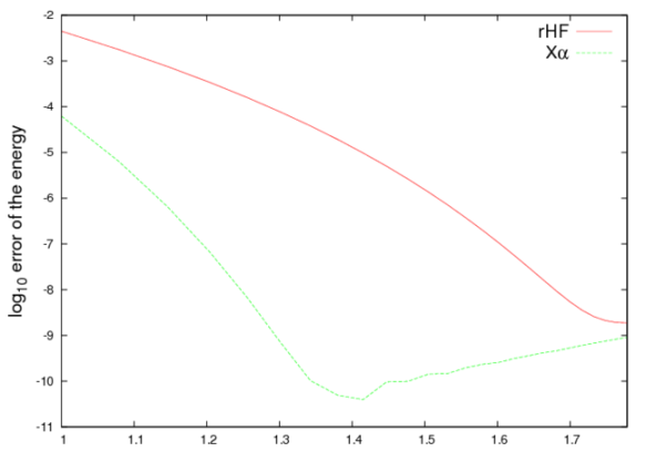
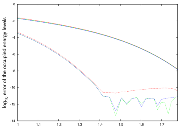
Figure 1: Log-log plot of the error on the total energy (left) and the three occupied energy levels (right) of the carbon atom for the rHF (solid lines) and ${\rm X}\alpha$ (dashed lines) models as a function of the cut-off radius $L_{e}$ for a fixed mesh size $N_{I}=50$ (the reference calculation corresponds to $L_{e}=100$ and $N_{I}=100$).

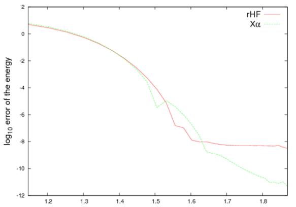
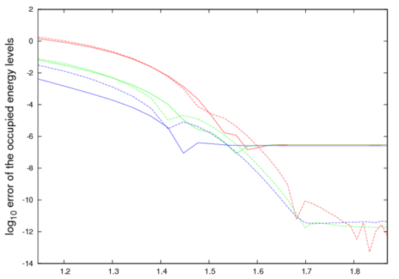
Figure 2: Log-log plot of the error on the total energy (left) and the three occupied energy levels (right) of the carbon atom for the rHF (solid lines) and ${\rm X}\alpha$ (dashed lines) models as a function of the mesh size $N_{I}$, for a fixed cut-off radius $L_{e}=50$ (the reference calculation corresponds to $L_{e}=100$ and $N_{I}=100$).

4.1 Electronic structures of isolated atoms

We report here calculations on all the atoms of the first four rows of the periodic table obtained with the rHF (Section 4.1.1) and X$\alpha$ (Section 4.1.2) models respectively.

4.1.1 Occupied energy levels in the rHF model

The negative eigenvalues of $H_{\rho^{0}}^{\rm rHF}$ for all $1\leq z\leq 54$ (first four rows of the periodic table) are listed in the tables below. The results for $1\leq z\leq 20$, $27\leq z\leq 39$, $43\leq z\leq 45$ and $48\leq z\leq 54$ correspond to $N_{I}$ increasing from $35$ to $75$ as $z$ increases and $L_{e}$ increasing from $30$ to $100$ as $|\epsilon_{z,z,\rm F}^{0,\rm rHF}|$ decreases, which were sufficient to obtain an accuracy of $1\;\mu$Ha. The remaining atoms are more difficult to deal with because the Fermi level seems to be an accidentally degenerate eigenvalue of $H_{\rho^{0}}^{\rm rHF}$ associated with

• the 4p and 3d shells for $z=21$ and $z=22$;

• the 5s and 3d shells for $23\leq z\leq 26$, with a Fermi level very close (or possibly equal) to zero;

• the 5p and 4d shells for $z=40$, with a Fermi level very close (or possibly equal) to zero;

• the 6s and 4d shells for $z=41$ and $z=42$, with a Fermi level very close (or possibly equal) to zero;

• the 5s and 4d shells for $z=46$ and $z=47$.

Since the radial component of the highest occupied orbital typically vanishes as $e^{-\sqrt{2|\epsilon_{z,z,\rm F}^{0,\rm rHF}|}r}$ if $\epsilon_{z,N,\rm F}^{0,\rm rHF}<0$ and algebraically if $\epsilon_{z,z,\rm F}^{0,\rm rHF}=0$, a very large value of $L_{e}$ is needed for the atoms for which the Fermi level is very close or possibly equal to zero. For that case, we use a non-uniform grid with $N_{I}^{\prime}=80$ and $L_{e}^{\prime}=100$ as explained in Section 3.1.4 and glue to it a uniform one with $10$ points and length $L_{e}-L_{e}^{\prime}$ varying from $70$ to $700$. Lastly, we add to the basis a function with an unbounded support, equal to $L_{e}/r$ on $[L_{e},+\infty)$ (see Appendix for details). This was sufficient to obtain an accuracy of $10\;\mu$Ha.

When the accidental degeneracy involves an $s$-shell and since the density is radial, the problem of finding the occupation numbers at the Fermi level reduces to finding a single parameter $t_{0}\in[0,1]$, which encodes the amount of electrons on the upper $s$-shell. In other words, one can write

$$\rho^{0,\rm rHF}_{z,z}=\rho_{\rm f}+t_{0}\rho_{\rm s}+(1-t_{0})\rho_{\rm d},$$

where $\rho_{\rm f}$ is the density corresponding to the fully occupied shells, and where $\rho_{\rm s}$ and $\rho_{\rm d}$ are densities corresponding to the accidentally degenerate s and d shells. Using the same trick for accidentally degenerate p and d shells, we manage to obtain a self-consistent solution to the rHF equations, which is necessarily a ground state since the rHF model is convex in the density matrix.

In the following tables, we report the rHF occupied energy levels (in Ha) of all the atoms of the first four rows of the periodic table. In some cases, the Fermi level seems to be an accidentally degenerate eigenvalue:

• the 4p and 3d orbitals have the same energy for $z=21,22$;

• the 5s and 3d orbitals have the same energy for $23\leq z\leq 26$;

• the 5p and 4d orbitals have the same energy for $z=40$;

• the 6s and 4d orbitals have the same energy for $z=41,42$;

• the 5s and 4d orbitals have the same energy for $z=46,47$.

In all these cases, the occupation number $0\leq n\leq 2$ of the partially occupied d orbitals is also given.

Hydrogen and helium:

Atom	z	1s
H	1	-0.046222
He	2	-0.184889

First row:

Atom	z	1s	2s	2p
Li	3	-1.202701	-0.013221	-
Be	4	-2.902437	-0.043722	-
B	5	-5.407212	-0.164961	-0.002389
C	6	-8.555732	-0.265682	-0.012046
N	7	-12.390177	-0.384699	-0.027312
O	8	-16.912538	-0.522883	-0.047280
F	9	-22.123525	-0.680479	-0.071663
Ne	10	-28.023481	-0.857597	-0.100342

Second row:

Atom	z	1s	2s	2p	3s	3p
Na	11	-35.065314	-1.453872	-0.514340	-0.012474	-
Mg	12	-42.963178	-2.169348	-1.037891	-0.034036	-
Al	13	-51.833760	-3.118983	-1.789953	-0.135543	-0.002486
Si	14	-61.532179	-4.160128	-2.629056	-0.208803	-0.010768
P	15	-72.083951	-5.319528	-3.582422	-0.284199	-0.023431
S	16	-83.489746	-6.598489	-4.651551	-0.363585	-0.039746
Cl	17	-95.749535	-7.997404	-5.836930	-0.447628	-0.059401
Ar	18	-108.863191	-9.516434	-7.138772	-0.536669	-0.082233

Third row:

Atom	z	1s	2s	2p	3s	3p	4s
K	19	-123.093717	-11.413369	-8.815789	-0.866180	-0.326113	-0.009500
Ca	20	-138.233855	-13.478564	-10.658837	-1.225936	-0.596554	-0.024275

Atom	z	1s	2s	2p	3s	3p	4s	4p	3d	$n$ (3d)
Sc	21	-154.35864	-15.78538	-12.74151	-1.69002	-0.96964	-0.08646	-0.00262	-0.00262	0.0056
Ti	22	-171.13186	-17.95490	-14.69008	-1.91684	-1.11529	-0.08224	-0.00056	-0.00056	0.3076

Atom	z	1s	2s	2p	3s	3p	4s	5s	3d	$n$ (3d)
V	23	-188.77080	-20.24077	-16.75392	-2.15109	-1.26708	-0.07796	-0.00044	-0.00044	0.5662
Cr	24	-207.27457	-22.64280	-18.93275	-2.39225	-1.42402	-0.07027	-0.00021	-0.00021	0.7794
Mn	25	-226.64207	-25.15938	-21.22503	-2.63884	-1.58451	-0.06385	-0.00008	-0.00008	0.9886
Fe	26	-246.87446	-27.79250	-23.63263	-2.89238	-1.74975	-0.05831	-0.00001	-0.00001	1.1957

Atom	z	1s	2s	2p	3s	3p	4s	3d
Co	27	-267.97363	-30.54468	-26.15798	-3.15502	-1.92172	-0.05438	-0.00121
Ni	28	-289.94364	-33.42047	-28.80557	-3.43107	-2.10456	-0.05459	-0.00722
Cu	29	-312.78019	-36.41574	-31.57124	-3.71624	-2.29392	-0.05539	-0.01370
Zn	30	-336.48301	-39.53045	-34.45491	-4.01038	-2.48957	-0.05646	-0.02026

Atom	z	1s	2s	2p	3s	3p	3d	4s	4p
Ga	31	-361.309461	-43.037010	-37.727020	-4.576035	-2.951273	-0.264266	-0.165288	-0.002386
Ge	32	-387.039855	-46.711685	-41.164308	-5.182760	-3.449483	-0.533749	-0.229337	-0.010542
As	33	-413.704397	-50.583856	-44.796323	-5.856750	-4.011096	-0.860725	-0.293291	-0.022574
Se	33	-441.297733	-54.647174	-48.616891	-6.590128	-4.628856	-1.240224	-0.358794	-0.037413
Br	35	-469.815876	-58.896767	-52.621294	-7.377307	-5.297678	-1.668313	-0.426192	-0.054625
Kr	36	-499.256211	-63.329305	-56.806329	-8.214637	-6.014298	-2.142323	-0.495638	-0.073991

Fourth row:

Atom	z	1s	2s	2p	3s	3p	3d	4s	4p	5s	5p
Rb	37	-529.827018	-68.150675	-61.378353	-9.306434	-6.983328	-2.867015	-0.760103	-0.271916	-0.008742	-
Sr	38	-561.340511	-73.171957	-66.148672	-10.462839	-8.015158	-3.653051	-1.032665	-0.475893	-0.021586	-
Y	39	-593.866153	-78.461974	-71.186183	-11.752114	-9.178245	-4.569112	-1.383317	-0.757307	-0.076589	-0.002707

Atom	z	1s	2s	2p	3s	3p	3d	4s	4p	5s	5p	4d	$n$ (4d)
Zr	40	-627.17364	-83.77963	-76.25111	-12.93681	-10.23529	-5.37710	-1.58204	-0.89248	-0.07367	-0.00048	-0.00048	0.3207

Atom	z	1s	2s	2p	3s	3p	3d	4s	4p	5s	6s	4d	$n$ (4d)
Nb	41	-661.38533	-89.25420	-81.47185	-14.14588	-11.31538	-6.20667	-1.76423	-1.01284	-0.06267	-0.00014	-0.00014	0.5840
Mo	42	-696.51265	-94.89727	-86.85999	-15.39104	-12.43032	-7.06960	-1.94236	-1.13016	-0.04957	-0.000002	-0.000002	0.7983

Atom	z	1s	2s	2p	3s	3p	3d	4s	4p	5s	4d
Tc	43	-732.565071	-100.718115	-92.424856	-16.681758	-13.589644	-7.975384	-2.126544	-1.254159	-0.044554	-0.009444
Ru	44	-769.539351	-106.713582	-98.163269	-18.014957	-14.790336	-8.920979	-2.314092	-1.381847	-0.043203	-0.024185
Rh	45	-807.43252	-112.88067	-104.07224	-19.3877	-16.02956	-9.90351	-2.50245	-1.51046	-0.04269	-0.04081

Atom	z	1s	2s	2p	3s	3p	3d	4s	4p	5s	4d	$n$ (4d)
Pd	46	-846.21733	-119.19036	-110.12295	-20.77177	-17.27895	-10.89439	-2.66438	-1.61336	-0.03846	-0.03846	1.6655
Ag	47	-885.91821	-125.66905	-116.34159	-22.19282	-18.56438	-11.91967	-2.82492	-1.71460	-0.03379	-0.03379	1.9293

Atom	z	1s	2s	2p	3s	3p	3d	4s	4p	4d	5s	5p
Cd	48	-926.623485	-132.409803	-122.820764	-23.742846	-19.977847	-13.071777	-3.073669	-1.901671	-0.096713	-0.042861	-
In	49	-968.415517	-139.493172	-129.641175	-25.501835	-21.599353	-14.430695	-3.487846	-2.251916	-0.310885	-0.131665	-0.002570
Sn	50	-1011.130388	-146.755434	-136.639081	-27.305190	-23.264351	-15.832028	-3.900956	-2.599067	-0.517562	-0.181855	-0.010599
Sb	51	-1054.799726	-154.228103	-143.846051	-29.184036	-25.004010	-17.307019	-4.343505	-2.973930	-0.749756	-0.230820	-0.021622
Te	52	-1099.421697	-161.909103	-151.260063	-31.136080	-26.816070	-18.853453	-4.812921	-3.374212	-1.006149	-0.280095	-0.034651
I	53	-1144.994552	-169.796463	-158.879194	-33.159211	-28.698453	-20.469283	-5.307002	-3.797932	-1.285246	-0.330100	-0.049319
Xe	54	-1191.517037	-177.888737	-166.702039	-35.251891	-30.649647	-22.153023	-5.824212	-4.243727	-1.585928	-0.381026	-0.065446

Remark 3.

Our numerical simulations seem to show that for all $1\leq z\leq 54$, there are no unoccupied negative eigenvalues in the rHF ground states of neutral atoms.

We end this section by the following figures, which back up the conjecture that rHF atomic densities are decreasing radial functions of the distance to the nucleus.

Figure 3: The left figure is the plot of the densities of all the atoms $1\leq z\leq 54$ obtained with our code as a function of the distance to the nucleus, on the interval $[0,0.05]$. The right one is the plot of the logarithms of those densities on the interval $[0,50]$.

4.1.2 Occupied energy levels in the ${\rm X}\alpha$ model

The tables below provide the negative eigenvalues of the Kohn-Sham X$\alpha$ Hamiltonian (in Ha) for all the atoms of the first four rows of the periodic table . We observe that atoms $z$, with $23\leq z\leq 28$ and $41\leq z\leq 44$ have accidentally degenerate Fermi levels, the degeneracy occurring in all cases between an s-shell and a d-shell (4s-3d for $23\leq z\leq 28$, 5s-4d for $41\leq z\leq 44$) . All the results of this section are obtained for $L_{e}=30$ and $N_{I}$ increasing from $30$ to $75$ as $z$ increases.

Hydrogen and helium:

Atom	z	1s
H	1	-0.194250
He	2	-0.516968

First row:

Atom	z	1s	2s	2p
Li	3	-1.820596	-0.079032	-0.019804
Be	4	-3.793182	-0.170028	-0.045681
B	5	-6.502185	-0.305377	-0.100041
C	6	-9.884111	-0.457382	-0.157952
N	7	-13.946008	-0.628841	-0.221004
O	8	-18.690815	-0.820599	-0.289512
F	9	-24.120075	-1.032963	-0.363534
Ne	10	-30.234733	-1.266049	-0.443056

Second row:

Atom	z	1s	2s	2p	3s	3p
Na	11	-37.647581	-2.007737	-1.006028	-0.077016	-
Mg	12	-45.897000	-2.845567	-1.661300	-0.142129	-
Al	13	-55.080562	-3.877978	-2.507293	-0.251340	-0.071775
Si	14	-65.107293	-5.017013	-3.456703	-0.359121	-0.117813
P	15	-75.982880	-6.269749	-4.516571	-0.470070	-0.166674
S	16	-87.709076	-7.638741	-5.689399	-0.585627	-0.218875
Cl	17	-100.286615	-9.125221	-6.976378	-0.706438	-0.274567
Ar	18	-113.715864	-10.729883	-8.378170	-0.832845	-0.333798

Third row:

Atom	z	1s	2s	2p	3s	3p	4s	3d
K	19	-128.330888	-12.775422	-10.219106	-1.233137	-0.646636	-0.064460	-
Ca	20	-143.848557	-14.981138	-12.218289	-1.655845	-0.981391	-0.111359	-
Sc	21	-160.10133	-17.14580	-14.17782	-1.94114	-1.18677	-0.12562	-0.08993
Ti	22	-177.19446	-19.39840	-16.22419	-2.21070	-1.37630	-0.13516	-0.12742

Atom	z	1s	2s	2p	3s	3p	4s	3d	$n$ (3d)
V	23	-195.11079	-21.72028	-18.33888	-2.44810	-1.53340	-0.13684	-0.13684	0.6393
Cr	24	-213.87746	-24.14440	-20.55424	-2.68033	-1.68342	-0.13575	-0.13575	0.8873
Mn	25	-233.50875	-26.68762	-22.88690	-2.92165	-1.83995	-0.13474	-0.13474	1.1278
Fe	26	-254.00470	-29.35014	-25.33699	-3.17214	-2.00304	-0.13379	-0.13379	1.3622
Co	27	-275.36535	-32.13212	-27.90468	-3.43191	-2.17274	-0.13292	-0.13292	1.5918
Ni	28	-297.59075	-35.03372	-30.59009	-3.70102	-2.34907	-0.13212	-0.13212	1.8174

Atom	z	1s	2s	2p	3s	3p	3d	4s	4p
Cu	29	-320.711183	-38.088382	-33.426318	-4.010749	-2.562693	-0.157720	-0.138533	-
Zn	30	-344.885966	-41.471174	-36.586685	-4.519851	-2.969457	-0.348234	-0.185366	-
Ga	31	-370.087065	-45.140343	-40.030943	-5.188704	-3.532081	-0.685727	-0.290872	-0.070624
Ge	32	-396.206872	-48.991790	-43.654803	-5.906101	-4.139819	-1.064181	-0.386783	-0.114696
As	33	-423.248196	-53.026929	-47.459904	-6.673183	-4.794502	-1.487148	-0.481338	-0.158885
Se	33	-451.209748	-57.243491	-51.444139	-7.487710	-5.494354	-1.953579	-0.576513	-0.20426
Br	35	-480.090322	-61.639549	-55.605706	-8.347907	-6.237921	-2.462342	-0.673116	-0.251199
Kr	36	-509.889039	-66.213681	-59.943283	-9.252538	-7.024197	-3.012574	-0.771572	-0.299874

Fourth row:

Atom	z	1s	2s	2p	3s	3p	3d	4s	4p	5s	4d
Rb	37	-540.863861	-71.219637	-64.711316	-10.452293	-8.104015	-3.854833	-1.088064	-0.547366	-0.061487	-
Sr	38	-572.774871	-76.418197	-69.670502	-11.708284	-9.238678	-4.750868	-1.407019	-0.798079	-0.102737	-
Y	39	-605.539841	-81.718973	-74.731216	-12.932519	-10.340292	-5.612293	-1.651693	-0.980422	-0.120721	-0.071919
Zr	40	-639.200123	-87.167101	-79.938205	-14.171025	-11.455022	-6.485549	-1.873159	-1.141874	-0.131037	-0.111534

Atom	z	1s	2s	2p	3s	3p	3d	4s	4p	5s	4d	$n$ (4d)
Nb	41	-673.74149	-92.74707	-85.27606	-15.40918	-12.56830	-7.35588	-2.05942	-1.27048	-0.13172	-0.13172	0.6535
Mo	42	-709.15136	-98.44597	-90.73190	-16.63439	-13.66757	-8.21062	-2.19877	-1.35425	-0.11937	-0.11937	0.9847
Tc	43	-745.48044	-104.31826	-96.35989	-17.90004	-14.80629	-9.10349	-2.34006	-1.43939	-0.10617	-0.10617	1.2956
Ru	44	-782.72787	-110.36286	-102.15896	-19.20531	-15.98365	-10.03361	-2.48279	-1.52544	-0.09183	-0.09183	1.5896

Atom	z	1s	2s	2p	3s	3p	3d	4s	4p	4d	5s	5p
Rh	45	-820.927173	-116.614569	-108.163817	-20.585170	-17.234646	-11.035987	-2.661143	-1.645733	-0.103288	-	-
Pd	46	-860.048546	-123.041777	-114.343011	-22.008434	-18.528092	-12.079263	-2.845456	-1.771555	-0.118970	-	-
Ag	47	-900.232540	-129.790427	-120.842024	-23.620128	-20.009041	-13.308869	-3.173860	-2.037653	-0.252103	-0.124136	-
Cd	48	-941.381019	-136.759252	-127.559951	-25.317963	-21.575259	-14.622541	-3.543470	-2.343065	-0.420723	-0.167825	-
In	49	-983.552576	-144.005647	-134.554225	-27.159345	-23.284171	-16.077676	-4.010922	-2.744597	-0.681578	-0.253924	-0.071162
Sn	50	-1026.665599	-151.449408	-141.744613	-29.062993	-25.054553	-17.593291	-4.493043	-3.159222	-0.954355	-0.330583	-0.110212
Sb	51	-1070.725180	-159.095276	-149.135914	-31.033521	-26.891049	-19.174056	-4.994724	-3.592188	-1.244953	-0.404626	-0.148390
Te	52	-1115.731902	-166.943588	-156.728514	-33.071174	-28.793930	-20.820270	-5.516439	-4.044198	-1.554330	-0.477952	-0.186783
I	53	-1161.685673	-174.994060	-164.522166	-35.175601	-30.762871	-22.531629	-6.058048	-4.515264	-1.882595	-0.551382	-0.225814
Xe	54	-1208.586286	-183.246330	-172.516543	-37.346393	-32.797483	-24.307764	-6.619330	-5.005277	-2.229668	-0.625352	-0.265689

We end this section by the following figures, which show that as in the ${\rm rHF}$ case, the ${\rm X}\alpha$ atomic densities seem to be decreasing radial functions of the distance to the nucleus.

Figure 4: The left figure is the plot of the ${\rm X}\alpha$ densities of all the atoms $1\leq z\leq 54$ obtained with our code as a function of the distance to the nucleus, on the interval $[0,0.05]$. The right one is the plot of the logarithms of those densities on the interval $[0,50]$.

4.2 Perturbation by a uniform electric field (Stark effect)

In this section, we consider atoms subjected to a uniform electric field, that is to an external potential $\beta W_{\rm Stark}$ with

$$W_{\rm Stark}(\mathbf{r})=-e_{\mathbf{z}}\cdot\mathbf{r},$$

or, in spherical coordinates,

$$W_{\rm Stark}(r,\theta,\varphi)=-\sqrt{\frac{4\pi}{3}}rY_{1}^{0}(\theta,\varphi).$$

As already mentioned in Section 2.2, $\widetilde{\mathcal{I}}_{z,N}^{\rm rHF/LDA}(\beta W_{\rm Stark})=-\infty$ whenever $\beta\neq 0$, and the corresponding variational problem has no minimizer. However, one can find a minimizer $\gamma_{h}\in{\mathcal{K}}_{N,h}$ to the approximated problem $\widetilde{\mathcal{I}}_{z,N,h}^{\rm rHF/LDA}(\beta W_{\rm Stark})$. Hereafter we consider the carbon atom ($z=6$). Even though the cutoff $m_{h}$ is set equal to $6$, all the terms corresponding to a magnetic number $m>1$ are in fact equal to zero.

The following figures are the plots in the $xy$-plane of the densities $\rho_{h}$ multiplied by $|\mathbf{r}|^{2}$ for the carbon atom ($z=6$) obtained for different values of $\beta$:

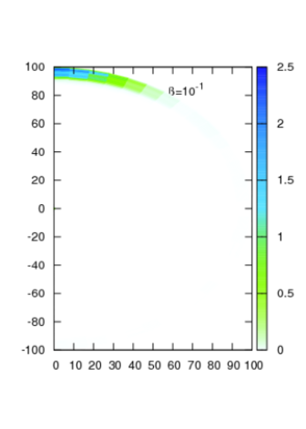
Figure 5: rHF case: the left figure is a plot of the density (multiplied by the function $(x^{2}+y^{2})$) of an isolated carbon atom. The other ones are plots of the densities (multiplied by the function $(x^{2}+y^{2})$) of the carbon atom subjected to a uniform external electric field, with coupling constants $\beta=10^{-3},10^{-2},10^{-1}$, respectively.

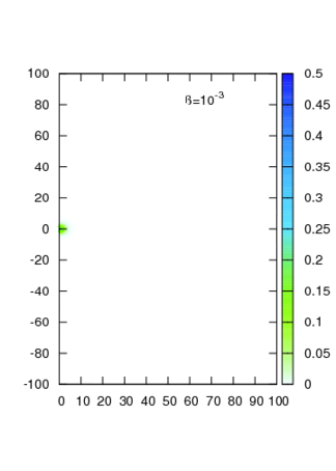
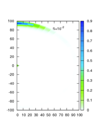
Figure 6: ${\rm X}\alpha$ case: The first figure is a plot of the density (multiplied by the function $(x^{2}+y^{2})$) of an isolated carbon atom. The other ones are plots of the densities (multiplied by the function $(x^{2}+y^{2})$) of the carbon atom subjected to a uniform external electric field, with coupling constants $\beta=10^{-3},10^{-2},10^{-1}$, respectively.

For $\beta=10^{-2}$ and $\beta=10^{-1}$, we clearly see spurious boundary effects: part of the electronic cloud is localized in the region where the external potential takes highly negative values. This result is obviously not physical. On the other hand, for the X$\alpha$ model and for $\beta=10^{-3}$ we simply observe a polarization of the electronic cloud. The perturbation potential being not spherically symmetric, it breaks the symmetry of the density. This numerical solution can probably be interpreted as a (nonlinear) resonant state. We will come back to the analysis of this interesting case in a following work.

Fig. 7 shows the amount of electrons of the carbon atom which escape to infinity as a function of the coupling constant $\beta$ (for $L_{e}=100$ and $N_{I}=50$), in the rHF and ${\rm X}\alpha$ case.

Figure 7: The upper figure is the plot of the integral on $B_{100}\setminus B_{50}$ of the density $\rho_{h}$, the lower left figure is the plot of the occupation number $n_{0,3}^{h}$, and the lower right one is the plot of the total energy, for $L_{e}=100$ and $N_{I}=50$ as a function of $\beta$ in the ${\rm rHF}$ and ${\rm X}\alpha$ cases.

In general, the standard ODA is used to achieve convergence (see Section 3). However, for $\beta$ small (resp. large) enough, the occupation numbers are selected as follows: $n_{0,1}^{[n]}=n_{0,2}^{[n]}=2$, $n_{0,3}=2(1-t_{0})$ and $n_{1,1}^{[n]}=2-n_{0,3}=2t_{0}$, $t_{0}$ being the minimizer of

$$t\mapsto\widetilde{E}_{6,6}^{\rm rHF/LDA}\left((1-t)\gamma^{[n]}_{0,*}+t\gamma^{[n]}_{1,*},\beta W\right),$$

where

$$\gamma^{[n]}_{0,*}=2\sum_{1\leq k\leq 3}|\Phi_{0,k,h}\rangle\langle\Phi_{0,k,h}|\quad\mbox{and}\quad\gamma^{[n]}_{1,*}=2\sum_{1\leq k\leq 2}|\Phi_{0,k,h}\rangle\langle\Phi_{0,k,h}|+2|\Phi_{1,1,h}\rangle\langle\Phi_{1,1,h}|.$$

This modification of ODA significantly increases the rate of convergence for $\beta$ small or large, but does not converge for all intermediate values of $\beta$.

While $\widetilde{\mathcal{I}}_{z,N}^{\rm rHF/LDA}(\beta W_{\rm Stark})=-\infty$ and the corresponding variational problem has no minimizer, the first-order perturbation $\gamma_{z,N,W_{\rm Stark}}^{(1),\rm rHF}$ of the ground state density matrix does exist (see Theorem 4). If we consider the carbon atom, it can be expressed as a function of the unperturbed occupied Kohn-Sham orbitals and of their first-order perturbations. We indeed have

$$\gamma_{6,6,W_{\rm Stark}}^{(1),\rm rHF}=\displaystyle\sum_{\underset{\underset{i_{1}+i_{2}+i_{3}=1}{i_{1}\geq 0,i_{2}\geq 0,i_{3}\geq 0}}{(m,k)\in{\mathcal{O}}_{6,6}}}n_{m,k}^{(i_{1})}|\Phi_{m,k}^{(i_{2})}\rangle\langle\Phi_{m,k}^{(i_{3})}|,$$

where ${\mathcal{O}}_{6,6}=\{(0,1),(0,2),(0,3),(1,1)\}$, where $\epsilon_{m,k}^{(0)}$ is the $k$-th lowest eigenvalue of $H_{6,6}^{0,\rm rHF}$ in the subspace ${\mathcal{H}}^{m}$, $\Phi_{m,k}^{(0)}$ an associated normalized eigenfunction and

$$n_{0,1}^{(0)}=n_{0,2}^{(0)}=2,\quad n_{0,3}^{(0)}=\frac{2}{3}\quad\mbox{and}\quad n_{1,1}^{(0)}=4/3,$$

while $\epsilon_{m,k}^{(1)}$, $\Phi_{m,k}^{(1)}$ and $n_{m,k}^{(1)}$ satisfy the following self-consistent equation

$$\left(H_{6,6}^{0,\rm rHF}-\epsilon_{m,k}^{(0)}\right)\Phi_{m,k}^{(1)}+\left(\rho^{(1)}\star|\cdot|^{-1}\right)\Phi_{m,k}^{(0)}+W_{\rm Stark}\Phi_{m,k}^{(0)}=\epsilon_{m,k}^{(1)}\Phi_{m,k}^{(0)},$$

$$\rho^{(1)}=\sum_{(m,k)\in{\mathcal{O}}_{6,6}}\!\!\!\!\!\!\!\!2\,n_{m,k}^{(0)}\Phi_{m,k}^{(0)}\Phi_{m,k}^{(1)}+n_{m,k}^{(1)}\Phi_{m,k}^{(0)}\Phi_{m,k}^{(0)},$$

$$\int_{{\mathbb{R}}^{3}}\Phi_{m,k}^{(1)}\Phi_{m,k}^{(0)}=0,\quad\mbox{and}\quad\sum_{(m,k)\in{\mathcal{O}}_{6,6}}n_{m,k}^{(1)}=0.$$

We denote by $\epsilon_{m,k,h}^{(0)}$, $\epsilon_{m,k,h}^{(1)}$, $\Phi_{m,k,h}^{(0)}$, $\Phi_{m,k,h}^{(1)}$ and $n_{m,k,h}^{(1)}$ the approximations of $\epsilon_{m,k}^{(0)}$, $\epsilon_{m,k}^{(1)}$, $\Phi_{m,k}^{(0)}$, $\Phi_{m,k}^{(1)}$ and $n_{m,k}^{(1)}$, respectively. For each $(m,k)\in{\mathcal{O}}_{6,6}$, define

$$\widetilde{\epsilon}_{m,k,h}^{(1)}(\beta):=\frac{1}{\beta}(\epsilon_{m,k,h}(\beta)-\epsilon_{m,k,h}^{(0)}),\quad\widetilde{\Phi}_{m,k,h}^{(1)}(\beta):=\frac{1}{\beta}(\Phi_{m,k,h}(\beta)-\Phi_{m,k,h}^{(0)}),\quad\mbox{and}\quad$$

$$\widetilde{n}_{m,k,h}^{(1)}(\beta):=\frac{1}{\beta}(n_{m,k,h}(\beta)-n_{m,k}^{(0)}).$$

Recall that, $\left(\Phi_{m,k,h}(\beta)\right)_{(m,k)\in{\mathcal{O}}_{6,6}}$ (resp. $n_{m,k,h}^{(1)}(\beta)$) are the eigenfunctions (resp. eigenvalues) of the density matrix $\gamma_{h}$, the minimizer of the approximated problem $\widetilde{\mathcal{I}}_{z,N,h}^{\rm rHF}(\beta W_{\rm Stark})$.

Let $U^{m,k}$ and $\widetilde{U}^{m,k}(\beta)$ be such that

$$\Phi_{m,k,h}^{(0)}(r,\theta,\varphi)=\sum_{l=|m|}^{m_{h}}\left(\sum_{i=1}^{N_{h}}U_{i,l}^{m,k}(\beta){\mathcal{X}}_{i}(r)/r\right)Y_{l}^{m}(\theta,\varphi)\quad\mbox{and}\quad$$

$$\widetilde{\Phi}_{m,k,h}^{(1)}(\beta)(r,\theta,\varphi)=\sum_{l=|m|}^{m_{h}}\left(\sum_{i=1}^{N_{h}}\widetilde{U}_{i,l}^{m,k}(\beta){\mathcal{X}}_{i}(r)/r\right)Y_{l}^{m}(\theta,\varphi).$$

To show that $\widetilde{\Phi}_{m,k,h}^{(1)}(\beta)\to\Phi_{m,k,h}^{(1)}$ when $\beta\to 0$, it is enough to show that for each $l\geq 0$

$$\left(\frac{1}{2}A+\frac{l(l+1)}{2}M_{-2}-zM_{-1}+NV_{\mu}-\epsilon^{(0)}M_{0}\right)\widetilde{U}_{.,l}(\beta)-\frac{1}{\sqrt{3}}C^{1,m}M_{1}U_{.,l-1}-\frac{1}{\sqrt{3}}C^{1,m}M_{1}U_{.,l+1}$$

$$+\sum_{l^{\prime}=|m|}^{m_{h}}\sum_{l^{\prime\prime}=0}^{2m_{h}}C^{l,m}_{l^{\prime},l^{\prime\prime}}([Q_{l^{\prime\prime}}]^{T}\cdot F)\widetilde{U}_{.,l^{\prime}}(\beta)+C^{l,m}_{l^{\prime},l^{\prime\prime}}([\widetilde{Q}_{l^{\prime\prime}}(\beta)]^{T}\cdot F)U_{.,l^{\prime}}-\epsilon^{(1)}M_{0}U_{.,l}\underset{\beta\rightarrow 0}{\rightarrow}0.$$ (59)

The index $(m,k)$ is omitted for simplicity and the vector $\widetilde{Q}_{l}(\beta)$ is the solution to the linear system

$$\left(A^{\rm a}+l(l+1)M_{-2}^{\rm a}\right)\widetilde{Q}_{l}=4\pi F:\widetilde{R}_{l},$$

with

$$\widetilde{R}_{l}:=\displaystyle\sum_{\underset{1\leq k\leq(m_{h}-|m|+1)\times N_{h}}{-m_{h}\leq m\leq m_{h}}}2n_{m,k}^{(0)}\widetilde{U}^{m,k}C^{l,m}[\widetilde{U}^{m,k}]^{T}+n_{m,k}^{(1)}\widetilde{U}^{m,k}C^{l,m}[U^{m,k}]^{T}.$$

Our numerical results show that, as expected by symmetry, $n_{m,k,h}^{(1)}=\epsilon_{m,k,h}^{(1)}=0$ for all $(m,k)\in{\mathcal{O}}_{6,6}$, and that the left-hand side of (59) converges to zero linearly in $\beta$ (see Fig.8).

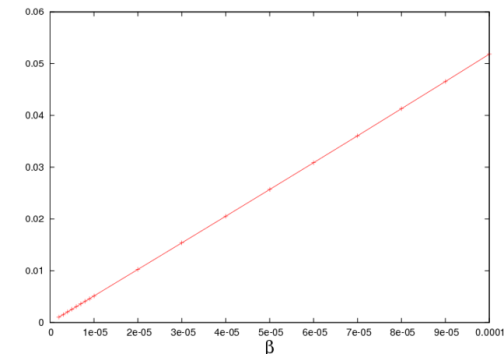
Figure 8: Plot of the function $\beta\mapsto\max_{(m,k)\,|\;n_{m,k}>0}\max_{l\geq|m|}\|V_{l,(m,k)}(\beta)\|_{\infty}$ where $V_{l,(m,k)}(\beta)$ is the vector in the left-hand side of (59).

5 Acknowledgements

The authors are grateful to Carlos García-Cervera and Vikram Gavini for valuable discussions.

Appendix: ${\mathbb{P}}4$ radial finite elements

In this appendix, we elaborate on the details of the calculation.

A1. Basis functions

We have chosen the following form functions to build the finite element matrices and tensors:

$$z_{1}(t)=1-t,\quad z_{2}(t)=t,\quad z_{3}(t)=4t(1-t)=-4t^{2}+4t,$$

$$z_{4}(t)=\frac{128}{3}t\left(\frac{1}{2}-t\right)\left(\frac{3}{4}-t\right)\left(1-t\right)=-\frac{128}{3}\left(t^{4}-\frac{9}{4}t^{3}+\frac{13}{8}t^{2}-\frac{3}{8}t\right),$$

$$z_{5}(t)=\frac{128}{3}t\left(t-\frac{1}{4}\right)\left(t-\frac{1}{2}\right)\left(1-t\right)=-\frac{128}{3}\left(t^{4}-\frac{7}{4}t^{3}+\frac{7}{8}t^{2}-\frac{1}{8}t\right).$$

Their derivatives are given by:

$$z_{1}^{\prime}(t)=-1,\quad z_{2}^{\prime}(t)=1,\quad z_{3}^{\prime}(t)=-8t+4,$$

$$z_{4}^{\prime}(t)=-\frac{128}{3}\left(4t^{3}-\frac{27}{4}t^{2}+\frac{13}{4}t-\frac{3}{8}\right),\quad z_{5}^{\prime}(t)=-\frac{128}{3}\left(4t^{3}-\frac{21}{4}t^{2}+\frac{7}{4}t-\frac{1}{8}\right).$$

Finite element basis:

• the 1D Schrödinger equation is solved on the finite interval $[0,L_{e}]$ with zero Dirichlet boundary conditions

• the interval $[0,L_{e}]$ is decomposed in $N_{I}$ intervals of positive lengths $h_{1},\cdots h_{N_{I}}$. Let $0=r_{1}<r_{2}<\cdots<r_{N_{I}}<r_{N_{I}+1}=L_{e}$ be such that $h_{k}=r_{k+1}-r_{k}$;

• we denote by

  $$V_{h}=\left\{v\in C^{0}([0,L_{e}])\mbox{ s.t. }v|_{[r_{k},r_{k+1}]}\in{\mathbb{P}}_{4},\quad v(0)=v(L_{e})=0\right\}$$

  the ${\mathbb{P}}_{4}$ finite element space associated with the so-defined mesh. We have

  $$\mbox{dim}(V_{h})=4N_{I}-1;$$

• we then set for all $1\leq k\leq N_{I}$ and $1\leq j\leq 5$,

  $$p^{k}_{j}(r)=z_{j}\left(\frac{r-r_{k}}{h_{k}}\right)$$

  so that $p^{k}_{j}(r_{k}+th_{k})=z_{j}(t)$, and define the basis $(\chi_{1},\cdots,\chi_{4N_{I}-1})$ of $V_{h}$ as follows:

  $$\chi_{1}(r)=p^{1}_{3}(r){\mathds{1}}_{[r_{1},r_{2}]},\quad\chi_{2}(r)=p^{1}_{4}(r){\mathds{1}}_{[r_{1},r_{2}]},\quad\chi_{3}(r)=p^{1}_{5}(r){\mathds{1}}_{[r_{1},r_{2}]},$$

  and for all $2\leq k\leq N_{I}$,

  $$\left\{\begin{array}[]{l}\displaystyle\chi_{4k-4}(r)=p^{k-1}_{2}(r){\mathds{1}}_{[r_{k-1},r_{k}]}+p^{k}_{1}(r){\mathds{1}}_{[r_{k},r_{k+1}]}\\ \chi_{4k-3}(r)=p^{k}_{3}(r){\mathds{1}}_{[r_{k},r_{k+1}]}\\ \chi_{4k-2}(r)=p^{k}_{4}(r){\mathds{1}}_{[r_{k},r_{k+1}]}\\ \chi_{4k-1}(r)=p^{k}_{5}(r){\mathds{1}}_{[r_{k},r_{k+1}]}\end{array}\right.$$

• when considering an atom with Fermi level very close or possible equal to zero, an extra basis function of the form

  $$\chi_{4N_{I}}(r)=p^{N_{I}}_{2}(r){\mathds{1}}_{[r_{N_{I}},r_{N_{I}+1}]}+\frac{r_{N_{I}+1}}{r}{\mathds{1}}_{[r_{N_{I}+1},\infty[}$$

  is added to the space $V_{h}$. Its derivative is equal to

  $$\chi_{4N_{I}}^{\prime}(r)=\frac{1}{h_{N_{I}}}{\mathds{1}}_{[r_{N_{I}},r_{N_{I}+1}[}-\frac{r_{N_{I}+1}}{r^{2}}{\mathds{1}}_{]r_{N_{I}+1},\infty[.}$$

A2. Assembling the matrices

Let $\Lambda$ be the bijective mapping from $\{0,1,2,3,4\}$ to $\{1,2,3,4,5\}$ defined by

$$\Lambda(0)=2,\quad\Lambda(1)=5,\quad\Lambda(2)=4,\quad\Lambda(3)=3,\quad\mbox{and}\quad\Lambda(4)=1.$$

Recall that the density is equal to

$$\rho_{h}(r,\theta)=\displaystyle\sum_{l=0}^{2m_{h}}\displaystyle\sum_{i,j=1}^{N_{h}}[R_{l}]_{i,j}\frac{{\mathcal{X}}_{i}(r)}{r}\frac{{\mathcal{X}}_{j}(r)}{r}Y_{l}^{0}(\theta).$$

Using the finite element basis defined above, one gets that $\rho_{h}(r,\theta)$ is equal to

$$\left|\begin{array}[]{rl}\displaystyle\sum_{l=0}^{2m_{h}}\displaystyle\sum_{i,j=0}^{3}[R_{l}]_{4-i,4-j}\frac{p^{1}_{\Lambda(i)}(r)}{r}\frac{p^{1}_{\Lambda(j)}(r)}{r}Y_{l}^{0}(\theta)&\quad\mbox{if}\quad r\in(r_{1},r_{2})\\ \\ \displaystyle\sum_{l=0}^{2m_{h}}\displaystyle\sum_{i,j=0}^{4}[R_{l}]_{4k-i,4k-j}\frac{p^{k}_{\Lambda(i)}(r)}{r}\frac{p^{k}_{\Lambda(j)}(r)}{r}Y_{l}^{0}(\theta)&\quad\mbox{if}\quad r\in(r_{k},r_{k+1}),\quad 1<k<N_{I}\\ \\ \displaystyle\sum_{l=0}^{2m_{h}}\displaystyle\sum_{i,j={\kappa}}^{4}[R_{l}]_{4N_{I}-i,4N_{I}-j}\frac{p^{N_{I}}_{\Lambda(i)}(r)}{r}\frac{p^{N_{I}}_{\Lambda(j)}(r)}{r}Y_{l}^{0}(\theta)&\quad\mbox{if}\quad r\in(r_{N_{I}},r_{N_{I}+1}),\end{array}\right.$$

where $\kappa$ equal to $1$ (resp. $0$) if the discretization space $V_{h}$ (resp. $V_{h}\cup\{\chi_{4N_{I}}\}$) is considered. In particular, for $0<t_{p,\rm r}<1$ and $-1<t_{q,\theta}<1$, we have that $(t_{p,\rm r}h_{k}+r_{k})^{2}\rho(t_{p,\rm r}h_{k}+r_{k},\arccos(t_{q,\theta}))$ is equal to

$$\left|\begin{array}[]{rl}\displaystyle\sum_{l=0}^{2m_{h}}\displaystyle\sum_{i,j=0}^{3}[R_{l}]_{4-i,4-j}z_{\Lambda(i)}(t_{p,\rm r})z_{\Lambda(j)}(t_{p,\rm r})\sqrt{\frac{2l+1}{4\pi}}P_{l}(t_{q,\theta})&\quad\mbox{if}\quad k=1\\ \\ \displaystyle\sum_{l=0}^{2m_{h}}\displaystyle\sum_{i,j=0}^{4}[R_{l}]_{4k-i,4k-j}z_{\Lambda(i)}(t_{p,\rm r})z_{\Lambda(j)}(t_{p,\rm r})\sqrt{\frac{2l+1}{4\pi}}P_{l}(t_{q,\theta})&\quad\mbox{if}\quad 1<k<N_{I}\\ \\ \displaystyle\sum_{l=0}^{2m_{h}}\displaystyle\sum_{i,j={\kappa}}^{4}[R_{l}]_{4N_{I}-i,4N_{I}-j}z_{\Lambda(i)}(t_{p,\rm r})z_{\Lambda(j)}(t_{p,\rm r})\sqrt{\frac{2l+1}{4\pi}}P_{l}(t_{q,\theta})&\quad\mbox{if}\quad k=N_{I},\end{array}\right.$$ (65)

where $P_{l}$ are the Legendre polynomials, which can be calculated using the recurrence relation

$$P_{n}(x)=\frac{2n-1}{n}xP_{n-1}(x)-\frac{n-1}{n}P_{n-2}(x),\quad n\geq 2,$$

with $P_{0}(x)=1$ and $P_{1}(x)=x$. Note that system (65) is used only to calculate the exchange-correlation potential, thus there is no need to define the density at radius greater than $r_{N_{I+1}}$.

For $\mu(r\mathbf{e})=\frac{\eta^{2}}{4\pi}\frac{e^{-\eta r}}{r}$, then

$$[V^{\rm H}(\mu)](r\mathbf{e})=\frac{1}{r}\left(1-e^{-\eta r}\right).$$

Thus the vector $G$ in (45) has one of the following form depending on the discretization space considered

$$G=\left[g^{1}_{3},g^{1}_{4},g^{1}_{5},\cdots,g^{k-1}_{2}+g^{k}_{1},g^{k}_{3},g^{k}_{4},g^{k}_{5},\cdots,g^{N_{I}-1}_{2}+g^{N_{I}}_{1},g^{N_{I}}_{3},g^{N_{I}}_{4},g^{N_{I}}_{5}\right]^{T},$$

or

$$G=\left[g^{1}_{3},g^{1}_{4},g^{1}_{5},\cdots,g^{k-1}_{2}+g^{k}_{1},g^{k}_{3},g^{k}_{4},g^{k}_{5},\cdots,g^{N_{I}-1}_{2}+g^{N_{I}}_{1},g^{N_{I}}_{3},g^{N_{I}}_{4},g^{N_{I}}_{5},g^{N_{I}}_{2}+g_{\infty}\right]^{T},$$

where

$$g_{i}^{k}=\frac{\eta^{2}}{4\pi}h_{k}e^{-\eta r_{k}}\int_{0}^{1}e^{-\eta th_{k}}z_{i}(t)\,dt$$

and

$$g_{\infty}=\frac{\eta^{2}}{4\pi}r_{N_{I+1}}\int_{r_{N_{I+1}}}^{\infty}\frac{e^{-\eta r}}{r}dr=\frac{\eta^{2}}{4\pi}r_{N_{I+1}}\int_{0}^{1}\frac{e^{\frac{-\eta r_{N_{I+1}}}{t}}}{t}\,dt.$$

We denote by

$$[\hat{\mathcal{H}}_{l,l^{\prime}}]=\sum_{l^{\prime\prime}=0}^{2m_{h}}C^{l,m}_{l^{\prime},l^{\prime\prime}}\left([Q_{l^{\prime\prime}}]^{T}\cdot F\right),$$ (66)

where $C^{l,m}$, $Q_{l}$ and $F$ are defined by (34), (42) and (44), respectively.

All the matrices $A$, $M_{-2}$, $M_{-1}$, $M_{0}$, $M_{1}$, $V_{\mu}$, $[V_{\rm xc}^{l}]$ and $[\hat{\mathcal{H}}_{l,l^{\prime}}]$ defined in (26), (37), (48) and (66), when considering the discretization space $V_{h}$, are symmetric and have the same pattern:

Their entries can be computed using elementary assembling matrices:

• diagonal blocks: for any $1\leq k\leq N_{I}$,

  $$\begin{array}[]{llll}Y_{4k-4,4k-4}=y^{k-1}_{22}+y^{k}_{11}&Y_{4k-4,4k-3}=y^{k}_{13}&Y_{4k-4,4k-2}=y^{k}_{14}&Y_{4k-4,4k-1}=y^{k}_{15}\\ Y_{4k-3,4k-4}=y^{k}_{31}&Y_{4k-3,4k-3}=y^{k}_{33}&Y_{4k-3,4k-2}=y^{k}_{34}&Y_{4k-3,4k-1}=y^{k}_{35}\\ Y_{4k-2,4k-4}=y^{k}_{41}&Y_{4k-2,4k-3}=y^{k}_{43}&Y_{4k-2,4k-2}=y^{k}_{44}&Y_{4k-2,4k-1}=y^{k}_{45}\\ Y_{4k-1,4k-4}=y^{k}_{51}&Y_{4k-1,4k-3}=y^{k}_{53}&Y_{4k-1,4k-2}=y^{k}_{54}&Y_{4k-1,4k-1}=y^{k}_{55}\end{array}$$

• off-diagonal blocks: for $1\leq k\leq N_{I}-1$

  $$Y_{4k-4,4k}=y^{k}_{12},\;Y_{4k-3,4k}=y^{k}_{23},\;Y_{4k-2,4k}=y^{k}_{24},\;Y_{4k-1,4k}=y^{k}_{25},$$

  $$Y_{4k,4k-4}=y^{k}_{21},\;Y_{4k,4k-3}=y^{k}_{32},\;Y_{4k,4k-2}=y^{k}_{42},\;Y_{4k,4k-1}=y^{k}_{52}.$$

When $\chi_{4N_{I}}$ is added to the discretization space, an extra row and an extra column must be added to each of the above matrices. The non-zero additional entries are:

$$Y_{4N_{I},4N_{I}}=y^{N_{I}}_{22}+y_{\infty},$$

$$Y_{4N_{I}-4,4N_{I}}=y^{N_{I}}_{12},\;Y_{4N_{I}-3,4N_{I}}=y^{N_{I}}_{23},\;Y_{4N_{I}-2,4N_{I}}=y^{N_{I}}_{24},\;Y_{4N_{I}-1,4N_{I}}=y^{N_{I}}_{25},$$

$$Y_{4N_{I},4N_{I}-4}=y^{N_{I}}_{21},\;Y_{4N_{I},4N_{I}-3}=y^{N_{I}}_{32},\;Y_{4N_{I},4N_{I}-2}=y^{N_{I}}_{42},\;Y_{4N_{I},4N_{I}-1}=y^{N_{I}}_{52}.$$

The $y^{k}_{ij}$’s are the entries of the elementary assembling matrices. The latter are defined for the matrices $A$, $M_{-2}$, $M_{-1}$, $M_{0}$, $M_{1}$, $V_{\mu}$, $[V_{\rm xc}^{l}]$ and $[\hat{\mathcal{H}}_{l,l^{\prime}}]$ as follows:

$$a^{k}_{ij} = \int_{r_{k}}^{r_{k+1}}{p^{k}_{i}}^{\prime}{p^{k}_{j}}^{\prime}=h_{k}^{-1}\int_{0}^{1}z_{i}^{\prime}z_{j}^{\prime}=h_{k}^{-1}\alpha_{ij}$$

$$(m_{-2})^{k}_{ij} = \int_{r_{k}}^{r_{k+1}}\frac{p^{k}_{i}(r)p^{k}_{j}(r)}{r^{2}}\,dr=h_{k}\int_{0}^{1}\frac{z_{i}(t)z_{j}(t)}{(r_{k}+th_{k})^{2}}\,dt$$

$$= \left|\begin{array}[]{ll}\displaystyle h_{k}r_{k}^{-2}\int_{0}^{1}\frac{z_{i}(t)z_{j}(t)}{(1+th_{k}/r_{k})^{2}}\,dt&\mbox{ if }k\geq 2\\ \displaystyle h_{1}^{-1}\int_{0}^{1}\frac{z_{i}(t)z_{j}(t)}{t^{2}}\,dt&\mbox{ if }k=1\end{array}\right.$$

$$(m_{-1})^{k}_{ij} = \int_{r_{k}}^{r_{k+1}}\frac{p^{k}_{i}(r)p^{k}_{j}(r)}{r}\,dr=h_{k}\int_{0}^{1}\frac{z_{i}(t)z_{j}(t)}{r_{k}+th_{k}}\,dt$$

$$= \left|\begin{array}[]{ll}\displaystyle h_{k}r_{k}^{-1}\int_{0}^{1}\frac{z_{i}(t)z_{j}(t)}{1+th_{k}/r_{k}}\,dt&\mbox{ if }k\geq 2\\ \displaystyle\int_{0}^{1}\frac{z_{i}(t)z_{j}(t)}{t}\,dt&\mbox{ if }k=1\end{array}\right.$$

$$(m_{0})^{k}_{ij} = \int_{r_{k}}^{r_{k+1}}p^{k}_{i}(r)p^{k}_{j}(r)dr=h_{k}\int_{0}^{1}z_{i}(t)z_{j}(t)dt=h_{k}\,\nu_{ij}$$

$$(m_{1})^{k}_{ij} = \int_{r_{k}}^{r_{k+1}}rp^{k}_{i}(r)p^{k}_{j}(r)dr=h_{k}^{2}\int_{0}^{1}tz_{i}(t)z_{j}(t)dt+h_{k}r_{k}\,\nu_{ij}=h_{k}^{2}\beta_{ij}+h_{k}r_{k}\,\nu_{ij}$$

$$(v_{\mu})_{ij}^{k} = (m_{-1})_{ij}^{k}-h_{k}e^{-\eta r_{k}}\int_{0}^{1}\frac{e^{-\eta th_{k}}}{r_{k}+th_{k}}z_{i}(t)z_{j}(t)\,dt$$

$$= \left|\begin{array}[]{ll}\displaystyle(m_{-1})^{k}-h_{k}r_{k}^{-1}e^{-\eta r_{k}}\int_{0}^{1}\frac{e^{-\eta th_{k}}}{1+th_{k}/r_{k}}z_{i}(t)z_{j}(t)\,dt&\mbox{ if }k\geq 2\\ \displaystyle(m_{-1})^{k}-e^{-\eta r_{k}}\int_{0}^{1}\frac{e^{-\eta th_{k}}}{t}z_{i}(t)z_{j}(t)\,dt&\mbox{ if }k=1\end{array}\right.$$

$$(v_{\rm xc}^{l})_{ij}^{k} = c_{\rm xc}h_{k}\sqrt{\frac{2l+1}{4\pi}}\displaystyle\sum_{p=1}^{N_{g,\rm r}}\displaystyle\sum_{q=1}^{N_{g,\theta}}\omega_{p}\omega_{q}^{\prime}\left(\rho(t_{p,\rm r}h_{k}+r_{k},\arccos(t_{q,\theta}))\right)^{\frac{1}{3}}P_{l}(t_{q,\theta})z_{i}(t_{p,\rm r})z_{j}(t_{p,\rm r})$$

$$= c_{\rm xc}\left|\begin{array}[]{rl}h_{k}r_{k}^{-1}\sqrt{\frac{2l+1}{4\pi}}\displaystyle\sum_{p=1}^{N_{g,\rm r}}\displaystyle\sum_{q=1}^{N_{g,\theta}}\omega_{p}\omega_{q}^{\prime}\left((t_{p,\rm r}h_{k}+r_{k})^{2}\rho(t_{p,\rm r}h_{k}+r_{k},\arccos(t_{q,\theta}))\right)^{\frac{1}{3}}\\ P_{l}(t_{q,\theta})\frac{z_{i}(t_{p,\rm r})z_{j}(t_{p,\rm r})}{t_{p,\rm r}h_{k}/r_{k}+1}(t_{p,\rm r}h_{k}+r_{k})^{\frac{1}{3}}\quad\mbox{ if }k\geq 2\\ \sqrt{\frac{2l+1}{4\pi}}\displaystyle\sum_{p=1}^{N_{g,\rm r}}\displaystyle\sum_{q=1}^{N_{g,\theta}}\omega_{p}\omega_{q}^{\prime}\left((t_{p,\rm r}h_{k})^{2}\rho(t_{p,\rm r}h_{k}+r_{k},\arccos(t_{q,\theta}))\right)^{\frac{1}{3}}\\ P_{l}(t_{q,\theta})\frac{z_{i}(t_{p,\rm r})z_{j}(t_{p,\rm r})}{t_{p,\rm r}}(t_{p,\rm r}h_{k})^{\frac{1}{3}}\quad\mbox{ if }k=1\end{array}\right.$$

in the ${\rm X}\alpha$-case, that is for $v_{\rm xc}(\rho)=-\left(\frac{3}{\pi}\right)^{\frac{1}{3}}\rho^{\frac{1}{3}}$,

$$(\hat{h}_{l,l^{\prime}})_{ij}^{k} = \left|\begin{array}[]{ll}\displaystyle\sum_{l^{\prime\prime}=0}^{2m_{h}}\sum_{n=1}^{3}c_{l,l^{\prime},l^{\prime\prime}}^{m}f_{ij\Lambda(n)}^{k}Q_{l^{\prime\prime},4-n}&\mbox{ if }k=1\\ \displaystyle\sum_{l^{\prime\prime}=0}^{2m_{h}}\sum_{n=0}^{4}c_{l,l^{\prime},l^{\prime\prime}}^{m}f_{ij\Lambda(n)}^{k}Q_{l^{\prime\prime},4k-n}&\mbox{ if }1<k<N_{I}\\ \displaystyle\sum_{l^{\prime\prime}=0}^{2m_{h}}\sum_{n={\kappa}}^{4}c_{l,l^{\prime},l^{\prime\prime}}^{m}f_{ij\Lambda(n)}^{k}Q_{l^{\prime\prime},4N_{I}-n}&\mbox{ if }k=N_{I},\end{array}\right.$$

where

$$f_{ijn}^{k}=\int_{r_{k}}^{r_{k+1}}\frac{p_{i}^{k}(r)p_{j}^{k}(r)p_{n}^{k}(r)}{r}dr=h_{k}\int_{0}^{1}\frac{z_{i}(t)z_{j}(t)z_{n}(t)}{(th_{k}+r_{k})}dt,$$

and

$$c_{\rm xc}=-\sqrt{\pi}\left(\frac{3}{\pi}\right)^{\frac{1}{3}}.$$

Note that $\rho(t_{p,\rm r}h_{k}+r_{k},\arccos(t_{q,\theta}))$ is calculated with the help of (65). The $y_{\infty}$ are defined for the matrices $A$, $M_{-2}$, $M_{-1}$, $M_{0}$, $V_{\mu}$ and $[\hat{H}_{l,l^{\prime}]}$ as follows:

$$a_{\infty}=\int_{r_{N_{I+1}}}^{\infty}\chi_{4N_{I}}^{\prime}\chi_{4N_{I}}^{\prime}=\int_{r_{N_{I+1}}}^{\infty}\frac{(r_{N_{I+1}})^{2}}{r^{4}}dr=\frac{1}{3r_{N_{I+1}}},$$

$$(m_{-2})_{\infty}=\int_{r_{N_{I+1}}}^{\infty}\frac{\chi_{4N_{I}}(r)\chi_{4N_{I}}(r)}{r^{2}}dr=\int_{r_{N_{I+1}}}^{\infty}\frac{(r_{N_{I+1}})^{2}}{r^{4}}dr=\frac{1}{3r_{N_{I+1}}},$$

$$(m_{-1})_{\infty}=\int_{r_{N_{I+1}}}^{\infty}\frac{\chi_{4N_{I}}(r)\chi_{4N_{I}}(r)}{r}dr=\int_{r_{N_{I+1}}}^{\infty}\frac{(r_{N_{I+1}})^{2}}{r^{3}}dr=\frac{1}{2},$$

$$(m_{0})_{\infty}=\int_{r_{N_{I+1}}}^{\infty}\chi_{4N_{I}}\chi_{4N_{I}}=\int_{r_{N_{I+1}}}^{\infty}\frac{(r_{N_{I+1}})^{2}}{r^{2}}dr=r_{N_{I+1}},$$

$$(v_{\mu})_{\infty} =\int_{r_{N_{I+1}}}^{\infty}\frac{1}{r}\left(1-e^{-\eta r}\right)\chi_{4N_{I}}(r)\chi_{4N_{I}}(r)dr=(m_{-1})_{\infty}-(r_{N_{I+1}})^{2}\int_{r_{N_{I+1}}}^{\infty}\frac{e^{-\eta r}}{r^{3}}dr$$

$$=(m_{-1})_{\infty}+\int_{0}^{1}e^{-\frac{\eta r_{N_{I+1}}}{t}}t\,dt,$$

and

$$(\hat{h}_{l,l^{\prime}})_{\infty}=\displaystyle\sum_{l^{\prime\prime}=0}^{2m_{h}}c_{l,l^{\prime},l^{\prime\prime}}^{m}f_{\infty}Q_{l^{\prime\prime},4N_{I}},$$

where $f_{\infty}=\int_{r_{N_{I+1}}}^{\infty}\frac{\chi_{4N_{I}}^{3}(r)}{r}dr=\int_{r_{N_{I+1}}}^{\infty}\frac{(r_{N_{I+1}})^{3}}{r^{4}}dr=\frac{1}{3}$.

In addition to assembling the matrices, we need to deal with the following term

$$\sum_{i,j=1}^{N_{h}}F_{ijn}[R_{l}]_{ij}$$

in order to calculate the right-hand side of (42). Let $k_{n}=1+\mbox{int}(\frac{n}{4})$ and $q_{n}=4-(n\,\mbox{mod}\,4)$, so that $n=4k_{n}-q_{n}$. Then the entries $\displaystyle\sum_{i,j=1}^{N_{h}}F_{ijn}[R_{l}]_{ij}$ of the vector $F:R_{l}$ are computed as follows

$$\left|\begin{array}[]{ll}\displaystyle\sum_{i,j=0}^{3}f_{\Lambda(i)\Lambda(j)\Lambda(q_{n})}^{1}[R_{l}]_{4-i,4-j}\quad\mbox{if}\quad k_{n}=1\\ \\ \displaystyle\sum_{i,j=0}^{4}f_{\Lambda(i)\Lambda(j)\Lambda(q_{n})}^{k_{n}}[R_{l}]_{4k_{n}-i,4k_{n}-j}\quad\mbox{if}\quad q_{n}\neq 4\quad\mbox{and}\quad 1<k_{n}<N_{I}\\ \\ \displaystyle\sum_{i,j={\kappa}}^{4}f_{\Lambda(i)\Lambda(j)\Lambda(q_{n})}^{N_{I}}[R_{l}]_{4N_{I}-i,4N_{I}-j}\quad\mbox{if}\quad q_{n}\neq 4\quad\mbox{and}\quad k_{n}=N_{I}\\ \\ \begin{array}[]{l}\displaystyle\sum_{i,j=0}^{3}f_{2\Lambda(i)\Lambda(j)}^{1}[R_{l}]_{4-i,4-j}+\displaystyle\sum_{i,j=0}^{4}f_{1\Lambda(i)\Lambda(j)}^{2}[R_{l}]_{8-i,8-j}\\ \quad\quad\quad\quad\quad\quad\quad\quad\quad\quad\quad\quad\quad\quad\quad\quad\quad\quad\mbox{if}\quad q_{n}=4\quad\mbox{and}\quad k=2\end{array}\\ \\ \begin{array}[]{c}\displaystyle\sum_{i,j=0}^{4}\left[f_{2\Lambda(i)\Lambda(j)}^{k_{n}-1}[R_{l}]_{4k_{n}-4-i,4k_{n}-4-j}\right.\\ \\ \left.+f_{1\Lambda(i)\Lambda(j)}^{k_{n}}[R_{l}]_{4k_{n}-i,4k_{n}-j}\right]\end{array}\quad\mbox{if}\quad q_{n}=4\quad\mbox{and}\quad 2<k<N_{I}\\ \\ \begin{array}[]{c}\displaystyle\sum_{i,j=0}^{4}f_{2\Lambda(i)\Lambda(j)}^{N_{I}-1}[R_{l}]_{4N_{I}-4-i,4N_{I}-4-j}\\ \\ +\displaystyle\sum_{i,j={\kappa}}^{4}f_{1\Lambda(i)\Lambda(j)}^{N_{I}}[R_{l}]_{4N_{I}-i,4N_{I}-j}\end{array}\quad\mbox{if}\quad q_{n}=4\quad\mbox{and}\quad k=N_{I}.\end{array}\right.$$

When the base $\chi_{4N_{I}}$ is added, the last entry of the vector $F:R_{l}$ is equal to

$$\left(F:R_{l}\right)_{N_{I}}=\displaystyle\sum_{i,j={\kappa}}^{4}f_{2\Lambda(i)\Lambda(j)}^{N_{I}}[R_{l}]_{4N_{I}-i,4N_{I}-j}+f_{\infty}[R_{l}]_{4N_{I},4N_{I}}.$$

We end this section by providing the values of $\alpha_{ij}$, $\beta_{ij}$ and $\nu_{ij}$, for $1\leq i,j\leq 5$,

$$\begin{array}[]{lllll}\alpha_{11}=1&\alpha_{12}=-1&\alpha_{13}=0&\alpha_{14}=0&\alpha_{15}=0\\ \alpha_{21}=-1&\alpha_{22}=1&\alpha_{23}=0&\alpha_{24}=0&\alpha_{25}=0\\ \alpha_{31}=0&\alpha_{32}=0&\alpha_{33}=16/3&\alpha_{34}=128/45&\alpha_{35}=128/45\\ \alpha_{41}=0&\alpha_{42}=0&\alpha_{43}=128/45&\alpha_{44}=3328/189&\alpha_{45}=5888/945\\ \alpha_{51}=0&\alpha_{52}=0&\alpha_{53}=128/45&\alpha_{54}=5888/945&\alpha_{55}=3328/189\end{array}$$

$$\begin{array}[]{lllll}\nu_{11}=1/3&\nu_{12}=1/6&\nu_{13}=1/3&\nu_{14}=4/15&\nu_{15}=4/45\\ \nu_{21}=1/6&\nu_{22}=1/3&\nu_{23}=1/3&\nu_{24}=4/45&\nu_{25}=4/15\\ \nu_{31}=1/3&\nu_{32}=1/3&\nu_{33}=8/15&\nu_{34}=64/315&\nu_{35}=64/315\\ \nu_{41}=4/15&\nu_{42}=4/45&\nu_{43}=64/315&\nu_{44}=128/405&\nu_{45}=128/2835\\ \nu_{51}=4/45&\nu_{52}=4/15&\nu_{53}=64/315&\nu_{54}=128/2835&\nu_{55}=128/405\end{array}$$

$$\begin{array}[]{lllll}\beta_{11}=1/12&\beta_{12}=1/12&\beta_{13}=2/15&\beta_{14}=16/315&\beta_{15}=16/315\\ \beta_{21}=1/12&\beta_{22}=1/4&\beta_{23}=1/5&\beta_{24}=4/105&\beta_{25}=68/315\\ \beta_{31}=2/15&\beta_{32}=1/5&\beta_{33}=4/15&\beta_{34}=16/315&\beta_{35}=16/105\\ \beta_{41}=16/315&\beta_{42}=4/105&\beta_{43}=16/315&\beta_{44}=64/945&\beta_{45}=64/2835\\ \beta_{51}=332/105&\beta_{52}=1852/105&\beta_{53}=592/63&\beta_{54}=704/315&\beta_{55}=704/2835.\end{array}$$

References

- [1] A. Anantharaman and E. Cancès. Existence of minimizers for Kohn-Sham models in quantum chemistry, Ann. I. H. Poincaré, An. 26 (2009) 2425–2455.
- [2] D. M. Brink and G. R. Satchler, Angular momentum, 3rd edition, Clarendon, Oxford, 1993.
- [3] E. Cancès and C. Le Bris, Can we outperform the DIIS approach for electronic structure calculations, Int. J. Quantum Chem. 79 (2000) 82-90.
- [4] E. Cancès and C. Le Bris, On the convergence of SCF algorithms for the Hartree-Fock equations, M2AN 34 (2000) 749-774
- [5] E. Cancès and N. Mourad, A mathematical perspective on density functional perturbation theory, Nonlinearity 27 (2014) 1999–2033.
- [6] E. Cancès and N. Mourad, Existence of a type of optimal norm-conserving pseudopotentials for Kohn-Sham models, Communications in Mathematical Sciences, Vol. 14, No. 5 (2016), pp. 1315-1352.
- [7] R. Dreizler and E.K.U Gross, Density functional theory, Springer Verlag, 1990.
- [8] D. Funaro, Polynomial approximation of differential equations, Springer-Verlag, 1992.
- [9] D. Gontier, -representability in noncollinear spin-polarized density functional theory, Phys. Rev. Lett. 111 (2013) 153001.
- [10] M. Hoffmann-Ostenhof and T. Hoffmann-Ostenhof, "Schrödinger inequalities" and asymptotic behavior of the electron density of atoms and molecules, Phys. Rev. A 16 (1977) 1782–1785.
- [11] W. Kohn and L.J. Sham, Self-consistent equations including exchange and correlation effects, Phys. Rev. 140 (1965) A1133–A1138.
- [12] J.P. Perdew, A. Zunger. Self-interaction correction to density-functional approximations for many-electron systems. Phys. Rev. B 23 (1981),5048–5079.
- [13] W.H. Press, S.A. Teukolsky, W.T. Vetterling and B.P. Flannery, Numerical recipes in Fortran 77. The art of scientific computing, 2nd edition, Cambridge University Press, 1992.
- [14] M. Reed and B. Simon, Methods of modern mathematical physics, Vol. IV: Analysis of operators, Academic Press, New York, 1978.
- [15] M. E. Rose. Elementary Theory of Angular Momentum, John Wiley Sons Inc.,New York, 1957.
- [16] J.C. Slater, A simplification of the Hartree-Fock method, Phys. Rev. 81 (1951) 385–390.
- [17] J.P. Solovej, Proof of the ionization conjecture in a reduced Hartree-Fock model, Invent. Math. 104 (1991) 291–311.
- [18] A. H. Stroud and D. Secrest, Gaussian Quadrature Formulas, Englewood Cliffs, NJ: Prentice-Hall, 1966.