Near optimal neural network estimator for spectral x-ray photon counting data with pileup

Abstract

Purpose: A neural network estimator to process x-ray spectral measurements from photon counting detectors with pileup. The estimator is used with an expansion of the attenuation coefficient as a linear combination of functions of energy multiplied by coefficients that depend on the material composition at points within the object [R.E. Alvarez and A. Macovski, Phys. Med. Biol., 1976, 733-744]. The estimator computes the line integrals of the coefficients from measurements with different spectra. Neural network estimators are trained with measurements of a calibration phantom with the clinical x-ray system. One estimator uses low noise training data and another network is trained with data computed by adding random noise to the low noise data. The performance of the estimators is compared to each other and to the Cramer-Rao lower bound (CRLB).

Methods: The estimator performance is measured using a Monte Carlo simulation with an idealized model of a photon counting detector that includes only pileup and quantum noise. Transmitted x-ray spectra are computed for a calibration phantom. The transmitted spectra are used to compute random data for photon counting detectors with pileup. Detectors with small and large dead times are considered. Neural network training data with extremely low noise are computed by averaging the random detected data with pileup for a large numbers of exposures of the phantom. Each exposure is equivalent to a projection image or one projection of a computed tomography scan. Training data with high noise are computed by using data from one exposure. Finally, training data are computed by adding random data to the low noise data. The added random data are multivariate normal with zero mean and covariance equal to the sample covariance of data for an object with properly chosen attenuation.

To test the estimators, random data are computed for different thicknesses of three test objects with different compositions. These are used as inputs to the neural network estimators. The mean squared errors (MSE), variance and square of the bias of the neural networks’ outputs with the random object data are each compared to the CRLB.

Results: The MSE for a network trained with low noise data and added noise is close to the CRLB for both the low and high pileup cases. Networks trained with very low noise data have low bias but large variance for both pileup cases. Networks trained with high noise data have both large bias and large variance.

Conclusion: With a properly chosen level of added training data noise, a neural network estimator for photon counting data with pileup can have variance close to the CRLB with negligible bias.

Key Words: spectral x-ray, photon counting, pileup, dual energy, Cramèr-Rao lower bound

1 INTRODUCTION

The estimator is used with the Alvarez-Macovski method¹. In this method, the x-ray attenuation coefficient is approximated as a linear combination of basis functions of energy multiplied by coefficients that depend only on the material composition at each point within the object. The estimator computes the line integrals of the coefficients from transmitted x-ray measurements with different energy spectra. Recently, neural networks have been suggested for this application^{2, 3, 4} by using the universal function approximation theorem⁵ to invert the nonlinear transformation from the the line integrals to the spectral measurements.

If the number of spectral measurements is equal to the number of basis functions then any estimator that inverts the deterministic transformation is the maximum likelihood estimator and it gives optimal performance^{1, 6, 7}. That is, in the limit of large photon counts it is unbiased and has covariance equal to the Cramer-Rao lower bound (CRLB)⁸. If the number of spectral measurements is greater than the number of basis functions then simply inverting the transformation does not necessarily give optimal results. For this case, the optimal estimator needs to use the probability distribution of the measurement noise to provide optimal performance⁹.

Systems with more spectral measurements than the number of basis functions are becoming increasingly important because of the introduction of photon counting detectors into medical x-ray imaging systems¹⁰. With these detectors, we can use pulse height analysis (PHA) to categorize the energy of individual photons into separate energy bins. The counts in each bin constitute a separate spectral measurement and the number of bins depends on technical factors of the detector design¹¹ but is typically larger than the basis set dimension.

There is no explicit way to incorporate the noise probability distribution with a neural network but in the past noise has been added to the training data to improve the generalizability of the network^{12, 13, 14, 15}. For our application, the noise variance varies exponentially with the variables being estimated and the off diagonal terms of the covariance also change with these variables¹⁶. Therefore, it is not clear whether adding noise to the training data will result in optimal performance and what is the proper level of noise to provide this performance. These questions are examined in this paper.

The approach used is to train the neural network with measurements of a calibration phantom in the clinical x-ray system. Low noise training data are computed by averaging together a large number (1000) of exposures of the phantom. Another set of training data is computed by adding zero mean multivariate normal random data with a covariance equal to the values on a properly chosen interior step of the calibration phantom to the low noise data. Training data with high noise are computed by using only one exposure. The output noise of neural network estimators trained with the three data sets are compared to each other and to the CRLB. Other factors that affect the estimator output noise include the number of steps in the calibration phantom as well as the architecture of the network.

Current state of the art photon counting detectors have defects including incomplete photon energy measurement due to K radiation and Compton scattered photon escape, charge sharing and trapping, polarization and other effects^{17, 10}. As the detector state of the art improves, we can expect these defects may be reduced to negligible levels. However, all photon counting detectors have a finite response time and, since the inter-arrival times of x-ray photons on the detector sensor are exponentially distributed¹⁸, there will always be a non-zero probability for two or more photons to enter the detector during its response time no matter how small. In addition, x-ray quantum noise is, of course, universal. In order to focus on these fundamental issues an idealized model that includes only quantum noise and pileup is used with a Monte Carlo simulation to test the neural network estimators’ performance.

Lee et al.² used a neural network estimator but did not examine noise in the output. Zimmerman and Schmidt^{19, 3} studied noise but used noisy training data from a single exposure of the calibration phantom. Touch et al.^{20, 4} used a neural network to correct projection data for defects and deadtime of photon counting detectors. They then reconstructed data from individual PHA bins to produce images of the object attenuation at a set of different x-ray energies instead of the basis set coefficient images produced by the estimator of this paper.

2 METHODS

2.A The estimation problem

For biological materials and an externally administered high atomic number contrast agent we need three or more functions to accurately approximate the attenuation coefficient²¹,

$$\mu(\mathbf{r},E)=a_{1}(\mathbf{r})f_{1}(E)+a_{2}(\mathbf{r})f_{2}(E)+a_{3}(\mathbf{r})f_{3}(E).$$ (1)

In this equation, $a_{i}(\mathbf{r})$ are the basis set coefficients, $f_{i}(E)$ are the basis functions and the subscripts are $i=1\ldots 3$. As implied by the notation, the basis set coefficients $a_{i}(\mathbf{r})$ are functions only of the position $\mathbf{r}$ within the object and the basis functions $f_{i}(E)$ are functions only of the x-ray energy $E$. Contrast agents with more than one high atomic number element may require additional functions of energy.

Neglecting scatter, the expected value of the number of transmitted photons $n_{k}$ for effective spectrum $S_{k}(E)$ is

$$\lambda_{k}=\left\langle n_{k}\right\rangle=\int S_{k}(E)e^{-\int\mu\left(\mathbf{r},E\right)d\mathbf{r}}dE,\ k=1\ldots n_{spect}$$ (2)

where $nspect$ is the number of spectral measurements, $\left\langle\ \right\rangle$ denotes expected value and the integral in the exponent is on a line from the x-ray source to the detector. With pulse height analysis the effective spectrum for an energy bin measurement can be idealized to be

$$S_{k}\left(E\right)=S_{incident}\left(E\right)\Pi_{k}\left(E\right)$$ (3)

where $S_{incident}\left(E\right)$ is the x-ray spectrum incident on the detector and $\Pi_{k}\left(E\right)$ is a rectangle function equal to one inside the energy bin and zero outside.

Using Eq. 1, the line integral in Eq. 2 can be expressed as

$$\int\mu\left(\mathbf{r},E\right)d\mathbf{r}=A_{1}f_{1}(E)+A_{2}f_{2}(E)+A_{3}f_{3}(E).$$ (4)

where $A_{i}=\int a_{i}\left(\mathbf{r}\right)d\mathbf{r},\ i=1\ldots 3$. The $A_{i}$ can be summarized as the components of the A-vector $\mathbf{A}$ and the measurements by a vector $\mathbf{N}$ whose components are the measurements with the effective spectra, $n_{k},\ k=1\ldots n_{spect}$. Since the x-ray transmission is exponential in $\mathbf{A}$, we can approximately linearize the measurements by taking logarithms. The results is the log measurement vector

$$\mathbf{L}=-\log(\mathbf{N/\mathbf{N_{0}}}),$$ (5)

where $\mathbf{N_{0}}$ is the expected value of the measurements with no object in the beam and the division means that corresponding elements of the vectors are divided.

Eq. 2 defines a relationship between $\mathbf{A}$ and the expected value of the measurement vector, $\mathbf{\left\langle L(A)\right\rangle}$. In an x-ray system, the objective of the estimator is to invert the relationship with noisy data and to compute the best estimate of the A-vector taking into account the probability distribution of the noise.

2.B The neural network estimator

The neural network shown in Fig. 1 was used as an estimator. The inputs to the network are the components of the $\mathbf{L}$ vector, Eq. 5. The network had one hidden layer with $12$ processing elements and three output elements, which are the estimates of the components of the A-vector, $\mathbf{A}$. This simple network was found to give near optimal performance due to the near linearity of the relationship between $\mathbf{L}$ and $\mathbf{A}.$ Other networks may also give good performance but they cannot have lower noise than the CRLB.

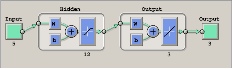
Figure 1: Neural network estimator block diagram. One hidden layer with $12$ processing elements and three output elements was found to give near optimal performance.

The hidden elements had a sigmoid response

$${\it sigmoid}(x)=\frac{2}{1+e^{-2x}}-1$$

and the output elements had a linear response.

The network was trained with calibration data measured with the clinical x-ray system as discussed in Sec. 2.C. The Levenberg-Marquardt algorithm was used for training. This algorithm selected the weights and offsets of the network to minimize the mean squared error of the estimates of the calibration phantom’s known A-vectors using the $\mathbf{L}$ data of the calibrator measured with the clinical x-ray system. During the training, random subsets of the data were used for training (70%), validation (15%), and final testing (15%). The stopping criterion was that the error with the validation set not decrease for six iterations or the maximum epochs, 500, were reached.

The neural network was used with all input data including those that fall outside the convex hull of the training data.

2.C The neural network training data

The neural network was trained using measurements of the calibration phantom shown in Fig. 2 with the clinical x-ray system. The figure shows a side-view of a three material phantom. The purpose of the calibration phantom is to provide values of the measurement vector $\mathbf{L}$ for a set of points in three dimensional A-space. If we use the attenuation coefficient functions of the materials of the calibrator as the basis set²², then the $\mathbf{A}$ vectors for each step are simply the thicknesses of the materials along lines from the x-ray source to the detector. The phantom can be constructed from stable, machinable materials such as acrylic plastic and aluminum. The third material could be, as an example, a plastic resin with molecular linked iodine whose attenuation simulates iodine contrast agent in blood²³.

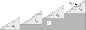
Figure 2: Three material calibration phantom. Step wedges of three materials with known thicknesses have known A-vectors at points in the three dimensional space. The transmitted flux through the calibration phantom is measured using the clinical x-ray system. The measurement data are stored by the system computer in a memory to be used to train the neural network as discussed in Sec. 2.B. See the estimator block diagram in Fig. 1.

The calibrator data are acquired with the clinical x-ray imaging system and do not require additional physics instruments that may be unavailable in clinical institutions. With a fan beam computed tomography system, the actual path lengths through different parts of phantom can be computed from its dimensions and the known geometry of the x-ray system by developing a method to locate the calibrator accurately with respect the the scanner gantry such as affixing pins to the phantom and scanning it. Fig. 2 shows a phantom with uniform steps but exponentially spaced thicknesses were used in the Monte Carlo simulations. They provide better results since they have closer spaced samples in the region near the origin where the gradient of $\mathbf{L(A)}$ is highest.

2.D Training with noisy data

The Monte Carlo simulation described in Sec. 2.I was used to study the optimal training data noise level. The noise was varied by adjusting the number of exposures averaged together for the training set where one exposure had the number of photons used for a clinical object image. Training data with low noise were computed by averaging 1000 trials. Alternate training data were computed by adding pseudo-random computer generated noise to the low noise data. The added data had a multivariate normal distribution with zero expected value vector. The covariance was the value for the photon counting detector data an A-vector with components equal to 0.05 of the maximum calibrator phantom thicknesses for each of the three materials. This covariance could be measured experimentally from the sample covariance for data from the calibration phantom for a step with this A-vector. Finally, high noise training data were computed by using only one exposure.

2.E Model for photon counting data with pulse pileup

The idealized model for photon counting data with pileup is described in detail in a previous paper¹⁶ and is summarized here. The response of photon counting detectors with pileup to an incident photon is modeled with the dead time parameter, $\tau$¹¹, which is the minimum time between two photons that are recorded as separate events. Two models are commonly used to describe the recorded counts with pileup: paralyzable and non-paralyzable. The non-paralyzable model is used in this paper. Measurements by Taguchi et al.²⁴ indicate it is more accurate at higher count rates with their detectors and it also leads to simpler analytical results²⁵.

A model is also needed for the recorded energies with pileup. One approach is to assume that the recorded energy is proportional to the integral of the sensor charge pulses during the dead time²⁴. An idealization of this model was used that assumes that the recorded energy is the sum of the energies of the photons that arrive during the dead time regardless of how close the arrival time of a photon to the end of the period²⁶. The idealized model assumes that the photon energy is converted completely into charge carriers so there are no losses due to Compton or Rayleigh scattering and all K-fluorescence radiation is re-absorbed within the sensor. All of the carriers are assumed to be collected so that there is no charge trapping or charge sharing with nearby detectors.

2.F Probability distribution of pulse height analysis data with pileup

Using the idealized pulse pileup model described in the previous Sec. 2.E, the probability distribution of PHA data with pileup is modeled as multivariate normal with the expected value and covariance in Table I^{26, 16}. The table has two columns, the first for data with no pileup and the second with pileup. In the table, the subscript ’rec’ denotes recorded data with pileup. The multivariate normal model can be shown to be accurate for the number of x-ray photons required for the measurements in material selective imaging¹⁶.

In the table,

$$\lambda=\int S_{incident\_det}(E)dE$$ (6)

is the expected value of the number of photons incident on the detector during the measurement time, $T$, and $\rho=\nicefrac{{\lambda}}{{T}}$ is the average rate of photon arrivals. The pileup parameter, $\eta=\rho\tau$, is the expected number of photons arriving during a dead time period, $\tau$. The total number of photons recorded by the detector in all PHA bins is $N_{rec}$ and the number recorded in PHA bin $k$ is $N_{rec,k}$. Notice that with non-zero pileup parameter the non-Poisson factor $D$ is not zero so the counts are not Poisson distributed. The formulas in the table were validated by a Monte Carlo simulation¹⁶.

Table I: PHA probability distribution. $\lambda$ is the expected number of photons incident on the detector during the measurement time, $\eta$ is the expected number of photons arriving during a dead time period, $N_{rec}$ is the total number of photons recorded by the detector in all PHA bins and $N_{rec,k}$ is the number recorded in PHA bin $k$.

	no pileup		with pileup
$\lambda=\int S_{incident\_det}(E)dE$	$\left\{0<E_{1}<\ldots<E_{nbins}\right\}$
photon number spectrum	$S(E)$		$S_{rec}(E)=\lambda p_{rec}(E)$
normalized spectrum	$p(E)=S(E)/\lambda$		$p_{rec}(E)=\sum_{k=0}^{\infty}\frac{\eta^{k}}{k!}e^{-\eta}\left(p^{(k)}*p\right)$
bin probabilities	$P_{k}=\int_{E_{k-1}}^{E_{k}}p(E)dE$		$P_{rec,k}=\int_{E_{k-1}}^{E_{k}}p_{rec}(E)dE$
expected total counts	$\left\langle N\right\rangle=\lambda$		$\left\langle N_{rec}\right\rangle=\frac{\lambda}{1+\eta}$
variance total counts	$var(N)=\lambda$		$var(N_{rec})=\frac{\lambda}{\left(1+\eta\right)^{3}}$
non-Poisson factor	$D=0$		$D=var(N_{rec})-\left\langle N_{rec}\right\rangle$
expected bin counts	$\left\langle N_{k}\right\rangle=\lambda P_{k}$		$\left\langle N_{rec,k}\right\rangle=\left\langle N_{rec}\right\rangle P_{rec,k}$
variance bin counts	$var(N_{k})=\lambda P_{k}$		$var(N_{rec,k})=\left\langle N_{rec}\right\rangle P_{rec,k}+DP_{rec,k}^{2}$
covariance bin counts	$0$		$cov(N_{j},N_{k})_{j\neq k}=P_{rec,j}P_{rec,k}D$

If the probability of a zero recorded photon count value is negligible, as is the case with the large expected values of counts required for material selective imaging, the parameters of the normal distribution of the logarithm $\mathbf{L}$ data²⁷ can be computed from the formulas in Table I using:

$$\begin{array}[]{ccc}\left\langle log(\mathbf{N})\right\rangle&=&log(\left\langle\mathbf{N}\right\rangle)\\ var\left(log(\mathbf{N})\right)&=&\frac{var\left(\mathbf{N}\right)}{\left\langle\mathbf{N}\right\rangle^{2}}\\ cov\left(log(\mathbf{N_{1}}),log(\mathbf{N_{2}})\right)&=&\frac{cov(\mathbf{N_{1},N_{2}})}{\left\langle\mathbf{N_{1}}\right\rangle\left\langle\mathbf{N_{2}}\right\rangle}.\end{array}$$ (7)

2.G The CRLB for A-vector noise with pileup

The CRLB is the minimum covariance for any unbiased estimator and is a fundamental limit from statistical estimator theory. It is the inverse of the Fisher information matrix $\mathbf{F}$ whose elements are²⁸

$$F_{ij}=-\left\langle\frac{\partial^{2}\mathcal{L}}{\partial A_{i}\partial A_{j}}\right\rangle$$ (8)

where $\mathcal{L}$ is the logarithm of the likelihood and the symbol $\left\langle\ \right\rangle$ denotes the expected value. Kay²⁹ shows that the Fisher information matrix for multivariate normal data with expected value $\mathbf{\left\langle L(A)\right\rangle}$ and covariance $\mathbf{C_{L}}$ has elements

$$\begin{array}[]{ccc}F_{ij}&=&\left[\frac{\partial\mathbf{\left\langle L(A)\right\rangle}}{\partial A_{i}}\right]^{T}\mathbf{C_{L}^{-1}}\left[\frac{\partial\mathbf{\left\langle L(A)\right\rangle}}{\partial A_{j}}\right]+\ldots\\ &&\frac{1}{2}tr\left[\mathbf{C_{L}^{-1}}\frac{\partial\mathbf{C_{L}}}{\partial A_{i}}\mathbf{C_{L}^{-1}}\frac{\partial\mathbf{C_{L}}}{\partial A_{j}}\right]\end{array}$$ (9)

where the $tr\left[\right]$ is the trace of a matrix.

The CRLB was computed numerically by approximating the derivatives in Eq. 9 from the first central difference. For example, to compute $\mathbf{\Delta L}$ we first compute the spectra through the object with attenuation $\mathbf{A}$ and then with $\mathbf{A+}\Delta\mathbf{A}$. The transmitted spectra are not affected by pileup since they occur before the measurement. These transmitted spectra are then used to compute the expected values of the measurements with pileup using the formulas in Sec. 2.F. We can similarly compute the difference of the covariance of the log data $\mathbf{C_{L}}$using the formulas in that section.

2.H The test object for Monte Carlo simulation

The performance of the neural network estimator was tested with objects with A-vectors on three lines through the A-vector space shown in Fig. 3. These correspond to a set of thicknesses of three uniform objects with different compositions. Each material has different basis set coefficients in its attenuation coefficient expansion, Eq. 1. Summarizing the coefficients as the components of the $\mathbf{a}$ vector, the line integrals are therefore $\mathbf{A=a}W$, where $W$ is the object thickness with units corresponding to attenuation coefficient, for example $g/cm^{2}$. The A-vectors for different thicknesses of a material therefore fall on a straight line through the origin in A-vector space. The end points of the lines used in the simulations, which also specify the ratios of the $\mathbf{a}$ vector coefficients, were $\left[16,\ 1.2,\ 0.1\right]$, $\left[5,\ 0.9,\ 0.1125\right]$, and $\left[16,\ 0.375,\ 0.1\right]$ $g/cm^{2}$. Fig. 3 shows a three dimension plot of the lines.

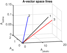
Figure 3: Three lines in A-vector space used in the Monte Carlo simulation. Each line is the A-vectors of different thicknesses of a material with a specific $\mathbf{a}$ vector of coefficients in its attenuation coefficient expansion.

2.I Random data for Monte Carlo simulation

The Monte Carlo simulation compared the mean squared error, the variance, and the square of the bias of the A-vector estimates to the Cramèr-Rao lower bound. The generation of the random data for the simulation started with the computation of a 120 kilovolt x-ray tube spectrum using the TASMIP algorithm of Boone and Seibert³⁰. The number of photons incident on the object for each detector element or pixel was set to $10^{6}$. The measurement time was assumed to be 10 milliseconds so the rate of photons incident on the detector with no object in the beam was $10^{8}$ photons per second. Two cases of pileup were computed by setting the detector dead times to 10 and 1 nanoseconds. These result in zero object thickness pileup parameters, $\eta_{0}$, of 1 and 0.1 respectively.

As discussed in Sec. 2.C, a basis set consisting of the attenuation coefficients of acrylic plastic, aluminum, and an iodine contrast agent simulant consisting of 20% fraction by weight iodine in paraffin ($C_{31}H_{64}$ molecular composition) was used as the basis functions of energy in Eq. 1. With this choice, the A-vectors were the thicknesses of each of the materials in the calibration phantom²². The attenuation coefficients of the materials were computed as the fraction by weight of each element in its chemical formula multiplied by the attenuation coefficient of that element. The elements’ attenuation coefficients were computed by piece-wise continuous Hermite polynomial interpolation of the standard Hubbell-Seltzer tables³¹.

A calibration phantom with 30 steps for each material was implemented. The thicknesses were geometrically spaced from zero to 20, 1.5 and 0.125 $g/cm^{2}$ for each of the calibration materials respectively. These were chosen to be greater than the object values so all $\mathbf{L}$ measurements except for noise will fall within the calibration data convex hull.

For a single A-vector on one of the lines in Fig. 3, the TASMIP x-ray tube spectrum was used with Eq. 6 to compute the spectrum and the expected value of the total number of transmitted photons incident on the detector sensor during the measurement time. The sensor was assumed to be perfectly absorbing so the signal for each photon was proportional to the photon energy. The recorded energy with pulse pileup was computed using the pileup model described in Sec. 2.E. Five bin PHA was done on the recorded energies. The PHA energy response functions were computed with an algorithm that maximized the SNR with no pileup and were assumed to be perfect rectangles. The algorithm for the optimal bins is described in a previous paper¹⁶.

The expected values and covariance of the recorded PHA bin counts were computed from the formulas in Table I. These were used to compute the parameters of the multivariate normal distributed log data $\mathbf{L}$ using Eq. 7. These data were used to test the neural network estimators.

2.J Estimator performance

The estimator performance was computed for the three training data sets and for the two cases of the dead time parameter, 1 and 10 nanoseconds. The neural networks were trained as described in Sec. 2.D. The input data to the estimators were computed as described in Sec. 2.I. The estimates of the networks were computed using the same random data as inputs so their output noise could be directly compared. The mean square error MSE of the estimates for 2000 trials was computed as

$$\mathbf{MSE}=\frac{1}{N_{trials}}\sum_{i=1}^{N_{trials}}\left(\hat{\mathbf{A}}-\mathbf{A_{actual}}\right)^{2}$$ (10)

where $N_{trails}$ is the number of trials, $\hat{A}$ is the estimate and $\mathbf{\mathbf{A_{actual}}}$ is the actual A-vector value. Notice that the MSE is a vector quantity with a value for each component of $\mathbf{A}$. The sample variance and the square of the sample bias of the estimates were also computed. These were plotted after normalizing by dividing by the CRLB variance.

3 RESULTS

3.A Mean squared error

Fig. 4 shows the mean squared errors of the neural network estimators as a function of A-vector magnitude for the three lines in Fig. 3. Panel (a) has the results for the low pileup case with zero object thickness dead time parameter, $\eta_{0}=0.1$, and panel (b) for the high pileup case, $\eta_{0}=1$. The A-vector magnitude is proportional to object thickness as explained in Sec. 2.H. The MSE with the two sets of training data noise were plotted using different symbols: 1000 trials averaged $\Diamond$ (low noise), added random noise $\ast$. The CRLB variance is plotted as the solid curves.

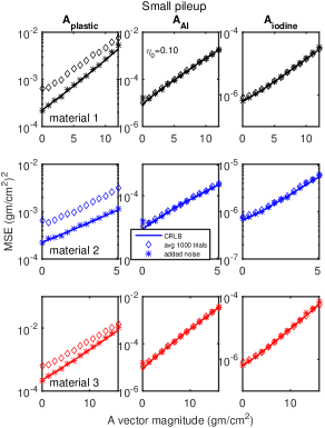
(a)(b)

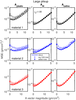
Figure 4: Mean squared error vs. A-vector magnitude for the (a) low zero object thickness pileup case, $\eta_{0}=0.1$, and (b) high pileup case, $\eta_{0}=1$. The errors are plotted as a function of the A-vector magnitude for the three lines in Fig. 3. The A-vector magnitude is proportional to object thickness as explained in Sec. 2.H. The results for each of the lines are in separate rows with the A-vector components in separate columns. The two sets of training data noise were plotted using different symbols: 1000 trials averaged,$\Diamond$ (low noise), and added random noise $\ast$.

3.B Variance

The variance of the neural network estimator outputs is shown in Fig. 5. Panel (a) shows the low pileup case, $\eta_{0}=0.1$, and panel (b) the high pileup case, $\eta_{0}=1$. The symbols for different training data sets are the same as in Fig. 4. For each A-vector component, the data are normalized by dividing by the CRLB variance and a dashed line is drawn at a ratio of one.

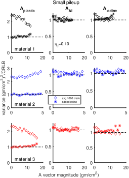
(a)   (b)

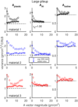
Figure 5: Variance for the (a) low zero object thickness pileup case, $\eta_{0}=0.1$, and (b) high pileup case, $\eta_{0}=1$, plotted as a function of A-vector magnitude. The symbols are the same as in Fig. 4. The data are normalized by dividing by the CRLB variance and a dashed line is drawn at a ratio of one. Notice that the neural network trained with low noise data has variance substantially larger than the networks trained with added noise.

3.C Bias

Fig. 6 shows the square of the bias for the two pileup cases. The bias squared data are normalized by dividing by the CRLB variance and a dashed line is drawn at a ratio of one.

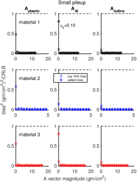
(a)(b)

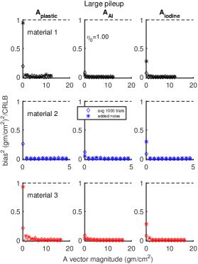
Figure 6: The square of the bias for the (a) low pileup case, $\eta_{0}=0.1$ and (b) high pileup case, $\eta_{0}=1$. See the caption of Fig. 5 for an explanation of the symbols. The data are normalized by dividing by the CRLB variance and a dashed line is drawn at a ratio of one.

3.D Bias and variance of network trained with high noise

Fig. 7 shows the bias and variance of a neural network trained with high noise data from a single exposure. The large pileup case is shown.

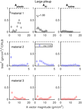
(a)(b)

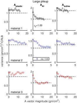
Figure 7: Bias (a) and variance (b) of network trained with high noise data with large pileup parameter. The data are normalized by dividing by the CRLB variance and a dashed line is drawn at a ratio of one.

4 DISCUSSION

Fig. 4 shows that, for either the small or large pileup cases, the neural network estimator trained with low noise data resulting from averaging 1000 exposures of the calibration phantom with added random noise has mean squared errors close to the CRLB. The network trained with low noise data only has MSE larger than the CRLB.

The mean squared error is equal to the variance plus the square of the bias and examining each of these components gives us insight into the effect of training data noise on the performance of the estimators. The variance results in Fig. 5 show that the low training data noise case, plotted as the diamonds has higher variance than the added noise case. The results in Fig. 6 show that both estimators have low bias.

Panel (b) of Fig. 4 shows that, with large pileup and for small thicknesses, the CRLB actually decreases as the object thickness increases. In the absence of pileup, we would expect that the A-vector noise variance and therefore the CRLB increases exponentially as the object thickness increases because the number of transmitted photons incident on the detector during the measurement time decreases exponentially. With pileup, the arrival rate of photons on the detector and therefore the pileup parameter also decrease exponentially with object thickness and, all other factors being equal, a decrease in the pileup parameter results in lower A-vector noise. The results indicate that in the small thickness region the decreased noise due to the improvement in the pileup parameter offsets the increase in noise due to fewer photons resulting in the decreased MSE shown in the figure.

Fig. 7 shows that a neural network trained with high noise data has both large bias and large variance.

The small dead time parameters used in the simulation, 10 and 1 nanosecond, are required to give the desired zero object thickness pileup parameters due to the large assumed arrival rate of $10^{8}$ photons/second. This rate, however, may be encountered at the edges of the body in computed tomography scanners¹⁰. The small dead times may be achievable in the future as sensor materials and detector electronics improve. Indeed, the performance of some current experimental systems is approaching these values. For example, Liu³² measured approximately 20 nanoseconds dead time for an experimental silicon strip sensor photon counting detector.

5 CONCLUSION

A neural network estimator trained with data with a properly chosen level of added noise can achieve near CRLB covariance with negligible bias. Training with low noise data results in low bias but large noise variance. A network trained with high noise data has both large bias and large variance.

References

- 1 R. E. Alvarez and A. Macovski, “Energy-selective reconstructions in X-ray computerized tomography,” Phys. Med. Biol. 21, 733–44, (1976). [Online]. Available: http://dx.doi.org/10.1088/0031-9155/21/5/002
- 2 W.-J. Lee, D.-S. Kim, S.-W. Kang, and W.-J. Yi, “Material depth reconstruction method of multi-energy x-ray images using neural network,” Proc. IEEE Engr. Med. Biol. Conf.,” 1514–1517, (Aug 2012). [Online]. Available: http://dx.doi.org/10.1109/EMBC.2012.6346229
- 3 K. C. Zimmerman and T. G. Schmidt, “Experimental comparison of empirical material decomposition methods for spectral ct,” Phys. Med. Biol. 60, no. 8, 3175, (2015). [Online]. Available: http://dx.doi.org/10.1088/0031-9155/60/8/3175
- 4 M. Touch, D. P. Clark, W. Barber, and C. T. Badea, “A neural network-based method for spectral distortion correction in photon counting x-ray ct,” Phys. Med.Biol. 61, no. 16, 6132, (2016). [Online]. Available: http://dx.doi.org/10.1088/0031-9155/61/16/6132
- 5 G. Cybenko, “Approximation by superpositions of a sigmoidal function,” Mathematics of Control, Signals and Systems 2, no. 4, 303–314, (1989). [Online]. Available: http://dx.doi.org/10.1007/BF02551274
- 6 R. E. Alvarez, “Estimator for photon counting energy selective x-ray imaging with multi-bin pulse height analysis,” Med. Phys. 38, 2324–2334, (2011). [Online]. Available: http://dx.doi.org/10.1118/1.3570658
- 7 R. E. Alvarez, “Efficient, non-iterative estimator for imaging contrast agents with spectral x-ray detectors,” IEEE Trans. Med. Imag.,” (2015). [Online]. Available: http://dx.doi.org/10.1109/TMI.2015.2510869
- 8 S. M. Kay, Fundamentals of Statistical Signal Processing, Volume I: Estimation Theory , Upper Saddle River, NJ: Prentice Hall PTR, 1993, Ch. 7.
- 9 S. M. Kay, Fundamentals of Statistical Signal Processing, Volume I: Estimation Theory , Upper Saddle River, NJ: Prentice Hall PTR, 1993.
- 10 K. Taguchi and J. S. Iwanczyk, “Vision 20/20: Single photon counting x-ray detectors in medical imaging,” Med. Phys. 40, 100901, (2013). [Online]. Available: http://dx.doi.org/10.1118/1.4820371
- 11 G. F. Knoll, Radiation Detection and Measurement, 3rd ed., Hoboken, N.J.: Wiley, 2000.
- 12 J. Sietsma and R. J. Dow, “Neural net pruning-why and how,” in Neural Networks, 1988., IEEE International Conference on, IEEE, 1988, 325–333. [Online]. Available: http://dx.doi.org/10.1109/ICNN.1988.23864
- 13 C. M. Bishop, “Training with Noise is Equivalent to Tikhonov Regularization,” Neural Computation 7, no. 1, 108–116, (Jan. 1995). [Online]. Available: http://dx.doi.org/10.1162/neco.1995.7.1.108
- 14 G. An, “The Effects of Adding Noise During Backpropagation Training on a Generalization Performance,” Neural Computation 8, no. 3, 643–674, (Apr. 1996). [Online]. Available: http://dx.doi.org/10.1162/neco.1996.8.3.643
- 15 R. M. Zur, Y. Jiang, L. L. Pesce, and K. Drukker, “Noise injection for training artificial neural networks: A comparison with weight decay and early stopping,” Med. Phys. 36, no. 10, 4810, (2009). [Online]. Available: http://dx.doi.org/10.1118/1.3213517
- 16 R. E. Alvarez, “Signal to noise ratio of energy selective x-ray photon counting systems with pileup,” Med. Phys. 41, no. 11, 111909, (2014). [Online]. Available: http://dx.doi.org/10.1118/1.4898102
- 17 M. Overdick, C. Baumer, K. J. Engel, J. Fink, C. Herrmann, H. Kruger, M. Simon, R. Steadman, and G. Zeitler, “Towards direct conversion detectors for medical imaging with X-rays,” IEEE Trans. Nucl. Sci. NSS08, 1527–1535, (2008). [Online]. Available: http://dx.doi.org/10.1109/NSSMIC.2008.4775117
- 18 H. H. Barrett and K. Myers, Foundations of Image Science, Hoboken, NJ: Wiley-Interscience, 2003, Ch.11.
- 19 K. C. Zimmerman, E. Y. Sidky, and T. Gilat Schmidt, “Experimental study of two material decomposition methods using multi-bin photon counting detectors,” Proc. SPIE 9033, 90 333G–6, (2014). [Online]. Available: http://dx.doi.org/10.1117/12.2043679
- 20 M. Touch, D. P. Clark, W. Barber, and C. T. Badea, “Novel approaches to address spectral distortions in photon counting x-ray CT using artificial neural networks,” in Proceedings SPIE, D. Kontos, T. G. Flohr, and J. Y. Lo, Eds., Apr. 2016, 97835P. [Online]. Available: http://proceedings.spiedigitallibrary.org/proceeding.aspx?doi=10.1117/12.2217037
- 21 R. E. Alvarez, “Dimensionality and noise in energy selective x-ray imaging,” Med. Phys. 40, no. 11, 111909, (2013). [Online]. Available: http://dx.doi.org/10.1118/1.4824057
- 22 R. E. Alvarez and E. J. Seppi, “A comparison of noise and dose in conventional and energy selective computed tomography,” IEEE Trans. Nucl. Sci. NS-26, 2853–2856, (1979). [Online]. Available: http://dx.doi.org/10.1109/TNS.1979.4330549
- 23 QRM-Gmbh, “QRM-CTiodine.” [Online]. Available: http://www.qrm.de/content/pdf/QRM-CTiodine.pdf
- 24 K. Taguchi, M. Zhang, E. C. Frey, X. Wang, J. S. Iwanczyk, E. Nygard, N. E. Hartsough, B. M. W. Tsui, and W. C. Barber, “Modeling the performance of a photon counting x-ray detector for CT: energy response and pulse pileup effects,” Med. Phys. 38, 1089–1102, (2011). [Online]. Available: http://dx.doi.org/10.1118/1.3539602
- 25 D. F. Yu and J. A. Fessler, “Mean and variance of single photon counting with deadtime,” Phys. Med. Biol. 45, 2043–2056, (2000). [Online]. Available: http://dx.doi.org/10.1088/0031-9155/45/7/324
- 26 A. S. Wang, D. Harrison, V. Lobastov, and J. E. Tkaczyk, “Pulse pileup statistics for energy discriminating photon counting x-ray detectors,” Med. Phys. 38, 4265–4275, (2011). [Online]. Available: http://dx.doi.org/10.1118/1.3592932
- 27 Papoulis, Athanasios, Probability, Random Variables, and Stochastic Processes, McGraw-Hill, 1965.
- 28 S. M. Kay, Fundamentals of Statistical Signal Processing, Volume I: Estimation Theory , Upper Saddle River, NJ: Prentice Hall PTR, 1993, Ch. 3.
- 29 S. M. Kay, Fundamentals of Statistical Signal Processing, Volume I: Estimation Theory , Upper Saddle River, NJ: Prentice Hall PTR, 1993, Sec. 4.5.
- 30 J. M. Boone and J. A. Seibert, “An accurate method for computer-generating tungsten anode x-ray spectra from 30 to 140 kV,” Med. Phys. 24, 1661–70, (1997). [Online]. Available: http://dx.doi.org/10.1118/1.597953
- 31 J. H. Hubbell, “Review of photon interaction cross section data in the medical and biological context,” Phys. Med. Biol. 44, R1–R22, (1999). [Online]. Available: http://dx.doi.org/10.1088/0031-9155/44/1/001
- 32 X. Liu, “Characterization and energy calibration of a silicon-strip detector for photon-counting spectral computed tomography,” Ph.D. dissertation, KTH Royal Institute of Technology, 2016. [Online]. Available: http://www.diva-portal.org/smash/record.jsf?pid=diva2:967342