Optimal Subsampling for Large Sample Logistic Regression

Abstract

For massive data, the family of subsampling algorithms is popular to downsize the data volume and reduce computational burden. Existing studies focus on approximating the ordinary least squares estimate in linear regression, where statistical leverage scores are often used to define subsampling probabilities. In this paper, we propose fast subsampling algorithms to efficiently approximate the maximum likelihood estimate in logistic regression. We first establish consistency and asymptotic normality of the estimator from a general subsampling algorithm, and then derive optimal subsampling probabilities that minimize the asymptotic mean squared error of the resultant estimator. An alternative minimization criterion is also proposed to further reduce the computational cost. The optimal subsampling probabilities depend on the full data estimate, so we develop a two-step algorithm to approximate the optimal subsampling procedure. This algorithm is computationally efficient and has a significant reduction in computing time compared to the full data approach. Consistency and asymptotic normality of the estimator from a two-step algorithm are also established. Synthetic and real data sets are used to evaluate the practical performance of the proposed method.

Keywords: $A$-optimality; Logistic Regression; Massive Data; Optimal Subsampling; Rare Event.

1 Introduction

With the rapid development of science and technologies, massive data have been generated at an extraordinary speed. Unprecedented volumes of data offer researchers both unprecedented opportunities and challenges. The key challenge is that directly applying statistical methods to these super-large sample data using conventional computing methods is prohibitive. We shall now present two motivating examples.

Example 1.

Census. The U.S. census systematically acquires and records data of all residents of the United States. The census data provide fundamental information to study socio-economic issues. Kohavi (1996) conducted a classification analysis using residents’ information such as income, age, work class, education, the number of working hours per week, and etc. They used these information to predict whether the residents are high income residents, i.e., those with annal income more than $\$50$K, or not. Given that the whole census data is super-large, the computation of statistical analysis is very difficult.

Example 2.

Supersymmetric Particles. Physical experiments to create exotic particles that occur only at extremely high energy densities have been carried out using modern accelerators. e.g., large Hadron Collider (LHC). Observations of these particles and measurements of their properties may yield critical insights about the fundamental properties of the physical universe. One particular example of such exotic particles is supersymmetric particles, the search of which is a central scientific mission of the LHC (Baldi et al., 2014). Statistical analysis is crucial to distinguish collision events which produce supersymmetric particles (signal) from those producing other particles (background). Since LHC continuously generates petabytes of data each year, the computation of statistical analysis is very challenging.

The above motivating examples are classification problems with massive data. Logistic regression models are widely used for classification in many disciplines, including business, computer science, education, and genetics, among others (Hosmer Jr et al., 2013). Given covariates ${\mathbf{x}}_{i}$’s $\in\mathbb{R}^{d}$, logistic regression models are of the form

$$P(y_{i}=1|{\mathbf{x}}_{i})=p_{i}(\boldsymbol{\beta})=\frac{\exp({\mathbf{x}}_{i}^{T}\boldsymbol{\beta})}{1+\exp({\mathbf{x}}_{i}^{T}\boldsymbol{\beta})},\quad i=1,2,...,n,$$ (1)

where $y_{i}$’s $\in\{0,1\}$ are the responses and $\boldsymbol{\beta}$ is a $d\times 1$ vector of unknown regression coefficients belonging to a compact subset of $\mathbb{R}^{d}$. The unknown parameter $\boldsymbol{\beta}$ is often estimated by the maximum likelihood estimator (MLE) through maximizing the log-likelihood function with respect to $\boldsymbol{\beta}$, namely,

$$\hat{{\boldsymbol{\beta}}}_{{{\textnormal{\tiny MLE}}}}=\arg\max_{{\boldsymbol{\beta}}}\ \ell({\boldsymbol{\beta}})=\arg\max_{{\boldsymbol{\beta}}}\ \sum_{i=1}^{n}\big{[}y_{i}\log p_{i}({\boldsymbol{\beta}})+(1-y_{i})\log\{1-p_{i}({\boldsymbol{\beta}})\}\big{]}.$$ (2)

Analytically, there is no general closed-form solution to the MLE $\hat{{\boldsymbol{\beta}}}_{{{\textnormal{\tiny MLE}}}}$, and iterative procedures are often adopted to find it numerically. A commonly used iterative procedure is Newton’s method. Specifically for logistic regression, Newton’s method iteratively applies the following formula until $\hat{{\boldsymbol{\beta}}}^{(t+1)}$ converges.

$$\hat{{\boldsymbol{\beta}}}^{(t+1)}=\hat{{\boldsymbol{\beta}}}^{(t)}+\left\{\sum_{i=1}^{n}w_{i}\Big{(}\hat{{\boldsymbol{\beta}}}^{(t)}\Big{)}{\mathbf{x}}_{i}{\mathbf{x}}_{i}^{T}\right\}^{-1}\frac{\partial\ell\Big{(}\hat{{\boldsymbol{\beta}}}^{(t)}\Big{)}}{\partial{\boldsymbol{\beta}}},$$

where $w_{i}({\boldsymbol{\beta}})=p_{i}({\boldsymbol{\beta}})\{1-p_{i}({\boldsymbol{\beta}})\}$. Since it requires $O(nd^{2})$ computing time in each iteration, the optimization procedure takes $O(\zeta nd^{2})$ time, where $\zeta$ is the number of iterations required for the optimization procedure to converge. One common feature of the two motivating examples is their super-large sample size. For such super-large sample problems, the computing time $O(nd^{2})$ for a single run may be too long to afford, let along to calculate it iteratively. Therefore, computation is a bottleneck for the application of logistic regression on massive data.

When proven statistical methods are no longer applicable due to limited computing resources, a popular method to extract useful information from data is the subsampling method (Drineas et al., 2006; Mahoney and Drineas, 2009; Drineas et al., 2011). This approach uses the estimate based on a subsample that is taken randomly from the full data to approximate the estimate from the full data. It is termed algorithmic leveraging in Ma et al. (2014, 2015) because the empirical statistical leverage scores of the input covariate matrix are often used to define the nonuniform subsampling probabilities. There are numerous variants of subsampling algorithms to solve the ordinary least squares (OLS) in linear regression for large data sets, see Drineas et al. (2006, 2011); Ma et al. (2014, 2015); Ma and Sun (2015), among others. Another strategy is to use random projections of data matrices to fast approximate the OLS estimate, which was studied in Rokhlin and Tygert (2008), Dhillon et al. (2013), Clarkson and Woodruff (2013) and McWilliams et al. (2014). The aforementioned approaches have been investigated exclusively within the context of linear regression, and available results are mainly on algorithmic properties. For logistic regression, Owen (2007) derived interesting asymptotic results for infinitely imbalanced data sets. King and Zeng (2001) investigated the problem of rare events data. Fithian and Hastie (2014) proposed an efficient local case-control (LCC) subsampling method for imbalanced data sets, in which the method was motivated by balancing the subsample. In this paper, we focus on approximating the full data MLE using a subsample, and our method is motivated by minimizing the asymptotic mean squared error (MSE) of the resultant subsample-estimator given the full data. We rigorously investigate the statistical properties of the general subsampling estimator and obtain its asymptotic distribution. More importantly, using this asymptotic distribution, we derive optimal subsampling methods motivated from the A-optimality criterion (OSMAC) in the theory of optimal experimental design.

In this paper, we have two major contributions for theoretical and methodological developments in subsampling for logistic regression with massive data:

1. Characterizations of optimal subsampling. Most work on subsampling algorithms (under the context of linear regression) focuses on algorithmic issues. One exception is the work by Ma et al. (2014, 2015), in which expected values and variances of estimators from algorithmic leveraging were expressed approximately. However, there was no precise theoretical investigation on when these approximations hold. In this paper, we rigorously prove that the resultant estimator from a general subsampling algorithm is consistent to the full data MLE, and establish the asymptotic normality of the resultant estimator. Furthermore, from the asymptotic distribution, we derive the optimal subsampling method that minimizes the asymptotic MSE or a weighted version of the asymptotic MSE.

2. A novel two-step subsampling algorithm. The OSMAC that minimizes the asymptotic MSEs depends on the full data MLE $\hat{{\boldsymbol{\beta}}}_{{{\textnormal{\tiny MLE}}}}$, so the theoretical characterizations do not immediately translate into good algorithms. We propose a novel two-step algorithm to address this issue. The first step is to determine the importance score of each data point. In the second step, the importance scores are used to define nonuniform subsampling probabilities to be used for sampling from the full data set. We prove that the estimator from the two-step algorithm is consistent and asymptotically normal with the optimal asymptotic covariance matrix under some optimality criterion. The two-step subsampling algorithm runs in $O(nd)$ time, whereas the full data MLE typically requires $O(\zeta nd^{2})$ time to run. This improvement in computing time is much more significant than that obtained from applying the leverage-based subsampling algorithm to solve the OLS in linear regression. In linear regression, compared to a full data OLS which requires $O(nd^{2})$ time, the leverage-based algorithm with approximate leverage scores (Drineas et al., 2012) requires $O(nd\log n/\varepsilon^{2})$ time with $\varepsilon\in(0,1/2]$, which is $o(nd^{2})$ for the case of $\log n=o(d)$.

The remainder of the paper is organized as follows. In section 2, we conduct a theoretical analyses of a general subsampling algorithm for logistic regression. In section 3, we develop optimal subsampling procedures to approximate the MLE in logistic regression. A two-step algorithm is developed in section 4 to approximate these optimal subsampling procedures, and its theoretical properties are studied. The empirical performance of our algorithms is evaluated by numerical experiments on synthetic and real data sets in Sections 5. Section 6 summarizes the paper. Technical proofs for the theoretical results, as well as additional numerical experiments are given in the Supplementary Materials.

2 General Subsampling Algorithm and its Asymptotic Properties

In this section, we first present a general subsampling algorithm for approximating $\hat{{\boldsymbol{\beta}}}_{{{\textnormal{\tiny MLE}}}}$, and then establish the consistency and asymptotic normality of the resultant estimator. Algorithm 1 describes the general subsampling procedure.

• Sampling: Assign subsampling probabilities $\pi_{i}$, $i=1,2,...n$, for all data points. Draw a random subsample of size $r\ (\ll n)$, according to the probabilities $\{\pi_{i}\}_{i=1}^{n}$, from the full data. Denote the covariates, responses, and subsampling probabilities in the subsample as ${\mathbf{x}}^{*}_{i}$, $y^{*}_{i}$, and $\pi_{i}^{*}$, respectively, for $i=1,2,...,r$.

• Estimation: Maximize the following weighted log-likelihood function to get the estimate $\tilde{{\boldsymbol{\beta}}}$ based on the subsample.

  $$\ell^{*}({\boldsymbol{\beta}})=\frac{1}{r}\sum_{i=1}^{r}\frac{1}{\pi_{i}^{*}}[y_{i}^{*}\log p_{i}^{*}({\boldsymbol{\beta}})+(1-y_{i}^{*})\log\{1-p_{i}^{*}({\boldsymbol{\beta}})\}],$$

  where $p_{i}^{*}({\boldsymbol{\beta}})={\exp({\boldsymbol{\beta}}^{T}{\mathbf{x}}_{i}^{*})}/\{1+\exp({\boldsymbol{\beta}}^{T}{\mathbf{x}}_{i}^{*})\}$. Due to the convexity of $\ell^{*}({\boldsymbol{\beta}})$, the maximization can be implemented by Newton’s method, i.e., iteratively applying the following formula until $\tilde{{\boldsymbol{\beta}}}^{(t+1)}$ and $\tilde{{\boldsymbol{\beta}}}^{(t)}$ are close enough,

  $$\tilde{{\boldsymbol{\beta}}}^{(t+1)}=\tilde{{\boldsymbol{\beta}}}^{(t)}+\left\{\sum_{i=1}^{r}\frac{w_{i}^{*}\big{(}\tilde{{\boldsymbol{\beta}}}^{(t)}\big{)}{\mathbf{x}}_{i}^{*}({\mathbf{x}}_{i}^{*})^{T}}{\pi_{i}^{*}}\right\}^{-1}\sum_{i=1}^{r}\frac{\big{\{}y_{i}^{*}-p_{i}^{*}\big{(}\tilde{{\boldsymbol{\beta}}}^{(t)}\big{)}\big{\}}{\mathbf{x}}_{i}^{*}}{\pi_{i}^{*}},$$ (3)

  where $w_{i}^{*}({\boldsymbol{\beta}})=p_{i}^{*}({\boldsymbol{\beta}})\{1-p_{i}^{*}({\boldsymbol{\beta}})\}$.

Algorithm 1 General subsampling algorithm

Now, we investigate asymptotic properties of this general subsampling algorithm, which provide guidance on how to develop algorithms with better approximation qualities. Note that in the two motivating examples, the sample sizes are super-large, but the numbers of predictors are unlikely to increase even if the sample sizes further increase. We assume that $d$ is fixed and $n\rightarrow\infty$. For easy of discussion, we assume that ${\mathbf{x}}_{i}$’s are independent and identically distributed (i.i.d) with the same distribution as that of ${\mathbf{x}}$. The case of nonrandom ${\mathbf{x}}_{i}$’s is presented in the Supplementary Materials. To facilitate the presentation, denote the full data matrix as ${\mathcal{F}_{n}}=({\mathbf{X}},{\mathbf{y}})$, where ${\mathbf{X}}=({\mathbf{x}}_{1},{\mathbf{x}}_{2},\dots,{\mathbf{x}}_{n})^{T}$ is the covariate matrix and ${\mathbf{y}}=(y_{1},y_{2},\dots,y_{n})^{T}$ is the vector of responses. Throughout the paper, $\|\mathbf{v}\|$ denotes the Euclidean norm of a vector $\mathbf{v}$, i.e., $\|\mathbf{v}\|=(\mathbf{v}^{T}\mathbf{v})^{1/2}$. We need the following assumptions to establish the first asymptotic result.

Assumption 1.

As $n\rightarrow\infty$, ${\mathbf{M}}_{X}=n^{-1}\sum_{i=1}^{n}w_{i}(\hat{{\boldsymbol{\beta}}}_{{{\textnormal{\tiny MLE}}}}){\mathbf{x}}_{i}{\mathbf{x}}_{i}^{T}$ goes to a positive-definite matrix in probability and $n^{-1}\sum_{i=1}^{n}\|{\mathbf{x}}_{i}\|^{3}=O_{P}(1)$.

Assumption 2.

$n^{-2}\sum_{i=1}^{n}\pi_{i}^{-1}\|{\mathbf{x}}_{i}\|^{k}=O_{P}(1)$ for $k=2,4$.

Assumption 1 imposes two conditions on the covariate distribution and this assumption holds if ${\mathrm{E}}({\mathbf{x}}{\mathbf{x}}^{T})$ is positive definite and ${\mathrm{E}}\|{\mathbf{x}}\|^{3}<\infty$. Assumption 2 is a condition on both subsampling probabilities and the covariate distribution. For uniform subsampling with $\pi_{i}=n^{-1}$, a sufficient condition for this assumption is that ${\mathrm{E}}\|{\mathbf{x}}\|^{4}<\infty$.

The theorem below presents the consistency of the estimator from the subsampling algorithm to the full data MLE.

Theorem 1.

If assumptions 1 and 2 hold, then as $n\rightarrow\infty$ and $r\rightarrow\infty$, $\tilde{{\boldsymbol{\beta}}}$ is consistent to $\hat{{\boldsymbol{\beta}}}_{{{\textnormal{\tiny MLE}}}}$ in conditional probability, given ${\mathcal{F}_{n}}$ in probability. Moreover, the rate of convergence is $r^{-1/2}$. That is, with probability approaching one, for any $\epsilon>0$, there exists a finite $\Delta_{\epsilon}$ and $r_{\epsilon}$ such that

$$P(\|\tilde{{\boldsymbol{\beta}}}-\hat{{\boldsymbol{\beta}}}_{{{\textnormal{\tiny MLE}}}}\|\geq r^{-1/2}\Delta_{\epsilon}|{\mathcal{F}_{n}})<\epsilon$$ (4)

for all $r>r_{\epsilon}$.

The consistency result shows that the approximation error can be made as small as possible by a large enough subsample size $r$, as the approximation error is at the order of $O_{P|{\mathcal{F}_{n}}}(r^{-1/2})$. Here the probability measure in $O_{P|{\mathcal{F}_{n}}}(\cdot)$ is the conditional measure given ${\mathcal{F}_{n}}$. This result has some similarity to the finite-sample result of the worst-case error bound for arithmetic leveraging in linear regression (Drineas et al., 2011), but neither of them gives the full distribution of the approximation error.

Besides consistency, we derive the asymptotic distribution of the approximation error, and prove that the approximation error, $\tilde{{\boldsymbol{\beta}}}-\hat{{\boldsymbol{\beta}}}_{{{\textnormal{\tiny MLE}}}}$, is asymptotically normal. To obtain this result, we need an additional assumption below, which is required by the Lindeberg-Feller central limit theorem.

Assumption 3.

There exists some $\delta>0$ such that $n^{-(2+\delta)}\sum_{i=1}^{n}{\pi_{i}^{-1-\delta}}{\|{\mathbf{x}}_{i}\|^{2+\delta}}=O_{P}(1)$.

The aforementioned three assumptions are essentially moment conditions and are very general. For example, a sub-Gaussian distribution (Buldygin and Kozachenko, 1980) has finite moment generating function on $\mathbb{R}$ and thus has finite moments up to any finite order. If the distribution of each component of ${\mathbf{x}}$ belongs to the class of sub-Gaussian distributions and the covariance matrix of ${\mathbf{x}}$ is positive-definite, then all the conditions are satisfied by the subsampling probabilities considered in this paper. The result of asymptotic normality is presented in the following theorem.

Theorem 2.

If assumptions 1, 2, and 3 hold, then as $n\rightarrow\infty$ and $r\rightarrow\infty$, conditional on ${\mathcal{F}_{n}}$ in probability,

$${\mathbf{V}}^{-1/2}(\tilde{{\boldsymbol{\beta}}}-\hat{{\boldsymbol{\beta}}}_{{{\textnormal{\tiny MLE}}}})\longrightarrow N(0,\mathbf{I})$$ (5)

in distribution, where

$${\mathbf{V}}={\mathbf{M}}_{X}^{-1}{\mathbf{V}}_{c}{\mathbf{M}}_{X}^{-1}=O_{p}(r^{-1})$$ (6)

and

$${\mathbf{V}}_{c}=\frac{1}{rn^{2}}\sum_{i=1}^{n}\frac{\{y_{i}-p_{i}(\hat{{\boldsymbol{\beta}}}_{{{\textnormal{\tiny MLE}}}})\}^{2}{\mathbf{x}}_{i}{\mathbf{x}}_{i}^{T}}{\pi_{i}}.$$ (7)

Remark.

Note that in Theorems 1 and 2 we are approximating the full data MLE, and the results hold for the case of oversampling ($r>n$). However, this scenario is not practical because it is more computationally intense than using the full data. Additionally, the distance between $\hat{{\boldsymbol{\beta}}}_{{{\textnormal{\tiny MLE}}}}$ and ${\boldsymbol{\beta}}_{0}$, the true parameter, is at the order of $O_{P}(n^{-1/2})$. Oversampling does not result in any gain in terms of estimating the true parameter. For aforementioned reasons, the scenario of oversampling is not of our interest and we focus on the scenario that $r$ is much smaller than $n$, typically, $n-r\rightarrow\infty$ or $r/n\rightarrow 0$.

Result (5) shows that the distribution of $\tilde{{\boldsymbol{\beta}}}-\hat{{\boldsymbol{\beta}}}_{{{\textnormal{\tiny MLE}}}}$ given ${\mathcal{F}_{n}}$ can be approximated by that of ${\mathbf{u}}$, a normal random variable with distribution $N({\bf 0},{\mathbf{V}})$. In other words, the probability $P(r^{1/2}\|\tilde{{\boldsymbol{\beta}}}-\hat{{\boldsymbol{\beta}}}_{{{\textnormal{\tiny MLE}}}}\|\geq\Delta|{\mathcal{F}_{n}})$ can be approximated by $P(r^{1/2}\|{\mathbf{u}}\|\geq\Delta|{\mathcal{F}_{n}})$ for any $\Delta$. To facilitate the discussion, we write result (5) as

$$\tilde{{\boldsymbol{\beta}}}-\hat{{\boldsymbol{\beta}}}_{{{\textnormal{\tiny MLE}}}}|{\mathcal{F}_{n}}\overset{a}{\sim}{\mathbf{u}},$$ (8)

where $\overset{a}{\sim}$ means the distributions of the two terms are asymptotically the same. This result is more statistically informative than a worst-case error bound for the approximation error $\tilde{{\boldsymbol{\beta}}}-\hat{{\boldsymbol{\beta}}}_{{{\textnormal{\tiny MLE}}}}$. Moreover, this result gives direct guidance on how to reduce the approximation error while an error bound does not, because a smaller bound does not necessarily mean a smaller approximation error.

Although the distribution of $\tilde{{\boldsymbol{\beta}}}-\hat{{\boldsymbol{\beta}}}_{{{\textnormal{\tiny MLE}}}}$ given ${\mathcal{F}_{n}}$ can be approximated by that of ${\mathbf{u}}$, this does not necessarily imply that ${\mathrm{E}}(\|\tilde{{\boldsymbol{\beta}}}-\hat{{\boldsymbol{\beta}}}_{{{\textnormal{\tiny MLE}}}}\|^{2}|{\mathcal{F}_{n}})$ is close to ${\mathrm{E}}(\|{\mathbf{u}}\|^{2}|{\mathcal{F}_{n}})$. ${\mathrm{E}}(\|{\mathbf{u}}\|^{2}|{\mathcal{F}_{n}})$ is an asymptotic MSE (AMSE) of $\tilde{\boldsymbol{\beta}}$ and it is always well defined. However, rigorously speaking, ${\mathrm{E}}(\|\tilde{{\boldsymbol{\beta}}}-\hat{{\boldsymbol{\beta}}}_{{{\textnormal{\tiny MLE}}}}\|^{2}|{\mathcal{F}_{n}})$, or any conditional moment of $\tilde{{\boldsymbol{\beta}}}$, is undefined, because there is a nonzero probability that $\tilde{{\boldsymbol{\beta}}}$ based on a subsample does not exist. The same problem exists in subsampling estimators for the OLS in linear regression. To address this issue, we define $\tilde{{\boldsymbol{\beta}}}$ to be 0 when the MLE based on a subsample does not exist. Under this definition, if $\tilde{{\boldsymbol{\beta}}}$ is uniformly integrable under the conditional measure given ${\mathcal{F}_{n}}$, $r^{1/2}\{{\mathrm{E}}(\|\tilde{{\boldsymbol{\beta}}}-\hat{{\boldsymbol{\beta}}}_{{{\textnormal{\tiny MLE}}}}\|^{2}|{\mathcal{F}_{n}})-{\mathrm{E}}(\|{\mathbf{u}}\|^{2}|{\mathcal{F}_{n}})\}\rightarrow 0$ in probability.

Results in Theorems 1 and 2 are distributional results conditional on the observed data, which fulfill our primary goal of approximating the full data MLE $\hat{{\boldsymbol{\beta}}}_{{{\textnormal{\tiny MLE}}}}$. Conditional inference is quite common in statistics, and the most popular method is the Bootstrap (Efron, 1979; Efron and Tibshirani, 1994). The Bootstrap (nonparametric) is the uniform subsampling approach with subsample size equaling the full data sample size. If $\pi_{i}=1/n$ and $r=n$, then results in Theorems 1 and 2 reduce to the asymptotic results for the Bootstrap. However, the Bootstrap and the subsampling method in the paper have very distinct goals. The Bootstrap focuses on approximating complicated distributions and are used when explicit solutions are unavailable, while the subsampling method considered here has a primary motivation to achieve feasible computation and is used even closed-form solutions are available.

3 Optimal Subsampling Strategies

To implement Algorithm 1, one has to specify the subsampling probability (SSP) $\boldsymbol{\pi}=\{\pi_{i}\}_{i=1}^{n}$ for the full data. An easy choice is to use the uniform SSP $\boldsymbol{\pi}^{\mathrm{UNI}}=\{\pi_{i}=n^{-1}\}_{i=1}^{n}$. However, an algorithm with the uniform SSP may not be “optimal” and a nonuniform SSP may have a better performance. In this section, we propose more efficient subsampling procedures by choosing nonuniform $\pi_{i}$’s to “minimize” the asymptotic variance-covariance matrix ${\mathbf{V}}$ in (6). However, since ${\mathbf{V}}$ is a matrix, the meaning of “minimize” needs to be defined. We adopt the idea of the $A$-optimality from optimal design of experiments and use the trace of a matrix to induce a complete ordering of the variance-covariance matrices (Kiefer, 1959). It turns out that this approach is equivalent to minimizing the asymptotic MSE of the resultant estimator. Since this optimal subsampling procedure is motivated from the A-optimality criterion, we call our method the OSMAC.

3.1 Minimum Asymptotic MSE of $\tilde{\boldsymbol{\beta}}$

From the result in Theorem 2, the asymptotic MSE of $\tilde{{\boldsymbol{\beta}}}$ is equal to the trace of ${\mathbf{V}}$, namely,

$$\mathrm{AMSE}(\tilde{{\boldsymbol{\beta}}})={\mathrm{E}}(\|{\mathbf{u}}\|^{2}|{\mathcal{F}_{n}})=\mathrm{tr}({\mathbf{V}}).$$ (9)

From (6), ${\mathbf{V}}$ depends on $\{\pi_{i}\}_{i=1}^{n}$, and clearly, $\{\pi_{i}=n^{-1}\}_{i=1}^{n}$ may not produce the smallest value of $\mathrm{tr}({\mathbf{V}})$. The key idea of optimal subsampling is to choose nonuniform SSP such that the $\mathrm{AMSE}(\tilde{{\boldsymbol{\beta}}})$ in (9) is minimized. Since minimizing the trace of the (asymptotic) variance-covariance matrix is called the $A$-optimality criterion (Kiefer, 1959), the resultant SSP is $A$-optimal in the language of optimal design. The following theorem gives the $A$-optimal SSP that minimizes the asymptotic MSE of $\tilde{\boldsymbol{\beta}}$.

Theorem 3.

In Algorithm 1, if the SSP is chosen such that

$$\pi_{i}^{\mathrm{mMSE}}=\frac{|y_{i}-p_{i}(\hat{{\boldsymbol{\beta}}}_{{{\textnormal{\tiny MLE}}}})|\|{\mathbf{M}}_{X}^{-1}{\mathbf{x}}_{i}\|}{\sum_{j=1}^{n}|y_{j}-p_{j}(\hat{{\boldsymbol{\beta}}}_{{{\textnormal{\tiny MLE}}}})|\|{\mathbf{M}}_{X}^{-1}{\mathbf{x}}_{j}\|},\;i=1,2,...,n,$$ (10)

then the asymptotic MSE of $\tilde{\boldsymbol{\beta}}$, $\mathrm{tr}({\mathbf{V}})$, attains its minimum.

As observed in (10), the optimal SSP $\boldsymbol{\pi}^{\mathrm{mMSE}}=\{\pi_{i}^{\mathrm{mMSE}}\}_{i=1}^{n}$ depends on data through both the covariates and the responses directly. For the covariates, the optimal SSP is larger for a larger $\|{\mathbf{M}}_{X}^{-1}{\mathbf{x}}_{i}\|$, which is the square root of the $i$th diagonal element of the matrix ${\mathbf{X}}{\mathbf{M}}_{X}^{-2}{\mathbf{X}}^{T}$. The effect of the responses on the optimal SSP depends on discrimination difficulties through the term $|y_{i}-p_{i}(\hat{{\boldsymbol{\beta}}}_{{{\textnormal{\tiny MLE}}}})|$. Interestingly, if the full data MLE $\hat{{\boldsymbol{\beta}}}_{{{\textnormal{\tiny MLE}}}}$ in $|y_{i}-p_{i}(\hat{{\boldsymbol{\beta}}}_{{{\textnormal{\tiny MLE}}}})|$ is replace by a pilot estimate, then this term is exactly the same as the probability in the local case-control (LCC) subsampling procedure in dealing with imbalanced data (Fithian and Hastie, 2014). However, Poisson sampling and unweighted MLE were used in the LCC subsampling procedure.

To see the effect of the responses on the optimal SSP, let $S_{0}=\{i:\ y_{i}=0\}$ and $S_{1}=\{i:\ y_{i}=1\}$. The effect of $p_{i}(\hat{{\boldsymbol{\beta}}}_{{{\textnormal{\tiny MLE}}}})$ on $\pi_{i}^{\mathrm{mMSE}}$ is positive for the $S_{0}$ set, i.e. a larger $p_{i}(\hat{{\boldsymbol{\beta}}}_{{{\textnormal{\tiny MLE}}}})$ results in a larger $\pi_{i}^{\mathrm{mMSE}}$, while the effect is negative for the $S_{1}$ set, i.e. a larger $p_{i}(\hat{{\boldsymbol{\beta}}}_{{{\textnormal{\tiny MLE}}}})$ results in a smaller $\pi_{i}^{\mathrm{mMSE}}$. The optimal subsampling approach is more likely to select data points with smaller $p_{i}(\hat{{\boldsymbol{\beta}}}_{{{\textnormal{\tiny MLE}}}})$’s when $y_{i}$’s are 1 and data points with larger $p_{i}(\hat{{\boldsymbol{\beta}}}_{{{\textnormal{\tiny MLE}}}})$’s when $y_{i}$’s are 0. Intuitively, it attempts to give preferences to data points that are more likely to be mis-classified. This can also be seen in the expression of $\mathrm{tr}({\mathbf{V}})$. From (6) and (7),

$$\mathrm{tr}({\mathbf{V}})= \mathrm{tr}({\mathbf{M}}_{X}^{-1}{\mathbf{V}}_{c}{\mathbf{M}}_{X}^{-1})$$

$$= \frac{1}{rn^{2}}\mathrm{tr}\left[\sum_{i=1}^{n}\frac{\{y_{i}-p_{i}(\hat{{\boldsymbol{\beta}}}_{{{\textnormal{\tiny MLE}}}})\}^{2}{\mathbf{M}}_{X}^{-1}{\mathbf{x}}_{i}{\mathbf{x}}_{i}^{T}{\mathbf{M}}_{X}^{-1}}{\pi_{i}}\right]$$

$$= \frac{1}{rn^{2}}\sum_{i=1}^{n}\frac{\{y_{i}-p_{i}(\hat{{\boldsymbol{\beta}}}_{{{\textnormal{\tiny MLE}}}})\}^{2}\mathrm{tr}({\mathbf{M}}_{X}^{-1}{\mathbf{x}}_{i}{\mathbf{x}}_{i}^{T}{\mathbf{M}}_{X}^{-1})}{\pi_{i}}$$

$$= \frac{1}{rn^{2}}\sum_{i\in S_{0}}\frac{\{p_{i}(\hat{{\boldsymbol{\beta}}}_{{{\textnormal{\tiny MLE}}}})\}^{2}\|{\mathbf{M}}_{X}^{-1}{\mathbf{x}}_{i}\|^{2}}{\pi_{i}}+\frac{1}{rn^{2}}\sum_{i\in S_{1}}\frac{\{1-p_{i}(\hat{{\boldsymbol{\beta}}}_{{{\textnormal{\tiny MLE}}}})\}^{2}\|{\mathbf{M}}_{X}^{-1}{\mathbf{x}}_{i}\|^{2}}{\pi_{i}}.$$

From the above equation, a larger value of $p_{i}(\hat{{\boldsymbol{\beta}}}_{{{\textnormal{\tiny MLE}}}})$ results in a larger value of the summation for the $S_{0}$ set, so a larger value is assigned to $\pi_{i}$ to reduce this summation. On the other hand for the $S_{1}$ set, a larger value of $p_{i}(\hat{{\boldsymbol{\beta}}}_{\textnormal{\tiny{ MLE}}})$ results in a smaller value of the summation, so a smaller value is assigned to $\pi_{i}$.

The optimal subsampling approach also echos the result in Silvapulle (1981), which gave a necessary and sufficient condition for the existence of the MLE in logistic regression. To see this, let

$$F_{0}=\left\{\sum_{i\in S_{0}}k_{i}{\mathbf{x}}_{i}\Big{|}k_{i}>0\right\}\quad\text{ and }\quad F_{1}=\left\{\sum_{i\in S_{1}}k_{i}{\mathbf{x}}_{i}\Big{|}k_{i}>0\right\}.$$

Here, $F_{0}$ and $F_{1}$ are convex cones generated by covariates in the $S_{0}$ and the $S_{1}$ sets, respectively. Silvapulle (1981) showed that the MLE in logistic regression is uniquely defined if and only if $F_{0}\cap F_{1}\neq\phi$, where $\phi$ is the empty set. From Theorem II in Dines (1926), $F_{0}\cap F_{1}\neq\phi$ if and only if there does not exist a ${\boldsymbol{\beta}}$ such that

$${\mathbf{x}}_{i}^{T}{\boldsymbol{\beta}}\leq 0\text{ for all }i\in S_{0},\quad{\mathbf{x}}_{i}^{T}{\boldsymbol{\beta}}\geq 0\text{ for all }i\in S_{1},$$ (11)

and at least one strict inequality holds. The statement in (11) is equivalent to the following statement in (12) below.

$$p_{i}({\boldsymbol{\beta}})\leq 0.5\text{ for all }i\in S_{0},\quad p_{i}({\boldsymbol{\beta}})\geq 0.5\text{ for all }i\in S_{1}.$$ (12)

This means if there exist a ${\boldsymbol{\beta}}$ such that $\{p_{i}({\boldsymbol{\beta}}),i\in S_{0}\}$ and $\{p_{i}({\boldsymbol{\beta}}),i\in S_{1}\}$ can be separated, then the MLE does not exist. The optimal subsampling SSP strives to increase the overlap of these two sets in the direction of $p_{i}(\hat{{\boldsymbol{\beta}}}_{{{\textnormal{\tiny MLE}}}})$. Thus it decreases the probability of the scenario that the MLE does not exist based on a resultant subsample.

3.2 Minimum Asymptotic MSE of ${\mathbf{M}}_{X}\tilde{\boldsymbol{\beta}}$

The optimal SSPs derived in the previous section require the calculation of $\|{\mathbf{M}}_{X}^{-1}{\mathbf{x}}_{i}\|$ for $i=1,2,...,n$, which takes $O(nd^{2})$ time. In this section, we propose a modified optimality criterion, under which calculating the optimal SSPs requires less time.

To motivate the optimality criteria, we need to define the partial ordering of positive definite matrices. For two positive definite matrices $\mathbf{A}_{1}$ and $\mathbf{A}_{2}$, $\mathbf{A}_{1}\geq\mathbf{A}_{2}$ if and only if $\mathbf{A}_{1}-\mathbf{A}_{2}$ is a nonnegative definite matrix. This definition is called the Loewner-ordering. Note that ${\mathbf{V}}={\mathbf{M}}_{X}^{-1}{\mathbf{V}}_{c}{\mathbf{M}}_{X}^{-1}$ in (6) depends on $\boldsymbol{\pi}$ through ${\mathbf{V}}_{c}$ in (7), and ${\mathbf{M}}_{X}$ does not depend on $\boldsymbol{\pi}$. For two given SSPs $\boldsymbol{\pi}^{(1)}$ and $\boldsymbol{\pi}^{(2)}$, ${\mathbf{V}}(\boldsymbol{\pi}^{(1)})\leq{\mathbf{V}}(\boldsymbol{\pi}^{(2)})$ if and only if ${\mathbf{V}}_{c}(\boldsymbol{\pi}^{(1)})\leq{\mathbf{V}}_{c}(\boldsymbol{\pi}^{(2)})$. This gives us guidance to simplify the optimality criterion. Instead of focusing on the more complicated matrix ${\mathbf{V}}$, we define an alternative optimality criterion by focusing on ${\mathbf{V}}_{c}$. Specifically, instead of minimizing $\mathrm{tr}({\mathbf{V}})$ as in Section 3.1, we choose to minimize $\mathrm{tr}({\mathbf{V}}_{c})$. The primary goal of this alternative optimality criterion is to further reduce the computing time.

The following theorem gives the optimal SSP that minimizes the trace of ${\mathbf{V}}_{c}$.

Theorem 4.

In Algorithm 1, if the SSP is chosen such that

$$\pi_{i}^{\mathrm{mVc}}=\frac{|y_{i}-p_{i}(\hat{{\boldsymbol{\beta}}}_{{{\textnormal{\tiny MLE}}}})|\|{\mathbf{x}}_{i}\|}{\sum_{j=1}^{n}|y_{j}-p_{j}(\hat{{\boldsymbol{\beta}}}_{{{\textnormal{\tiny MLE}}}})|\|{\mathbf{x}}_{j}\|},\ i=1,2,...,n,$$ (13)

then $\mathrm{tr}({\mathbf{V}}_{c})$, attains its minimum.

It turns out that the alternative optimality criterion indeed greatly reduces the computing time. From Theorem 4, the effect of the covariates on $\boldsymbol{\pi}^{\mathrm{mVc}}=\{\pi_{i}^{\mathrm{mVc}}\}_{i=1}^{n}$ is presented by $\|{\mathbf{x}}_{i}\|$, instead of $\|{\mathbf{M}}_{X}^{-1}{\mathbf{x}}_{i}\|$ as in $\boldsymbol{\pi}^{\mathrm{mMSE}}$. The computational benefit is obvious: it requires $O(nd)$ time to calculate $\|{\mathbf{x}}_{i}\|$ for $i=1,2,...,n$, which is significantly less than the required $O(nd^{2})$ time to calculate $\|{\mathbf{M}}_{X}^{-1}{\mathbf{x}}_{i}\|$ for $i=1,2,...,n$.

Besides the computational benefit, this alternative criterion also enjoys nice interpretations from the following aspects. First, the term $|y_{i}-p_{i}(\hat{{\boldsymbol{\beta}}}_{{{\textnormal{\tiny MLE}}}})|$ functions the same as in the case of $\boldsymbol{\pi}^{\mathrm{mMSE}}$. Hence all the nice interpretations and properties related to this term for $\boldsymbol{\pi}^{\mathrm{mMSE}}$ in Section 3.1 are true for $\boldsymbol{\pi}^{\mathrm{mVc}}$ in Theorem 4. Second, from (8),

$${\mathbf{M}}_{X}(\tilde{{\boldsymbol{\beta}}}-\hat{{\boldsymbol{\beta}}}_{{{\textnormal{\tiny MLE}}}})\big{|}{\mathcal{F}_{n}}\overset{a}{\sim}{\mathbf{M}}_{X}{\mathbf{u}},\text{ where }{\mathbf{M}}_{X}{\mathbf{u}}\sim N({\bf 0},{\mathbf{V}}_{c})\text{ given }{\mathcal{F}_{n}}.$$

This shows that $\mathrm{tr}({\mathbf{V}}_{c})={\mathrm{E}}(\|{\mathbf{M}}_{X}{\mathbf{u}}\|^{2}|{\mathcal{F}_{n}})$ is the AMSE of ${\mathbf{M}}_{X}\tilde{{\boldsymbol{\beta}}}$ in approximating ${\mathbf{M}}_{X}\hat{{\boldsymbol{\beta}}}_{{{\textnormal{\tiny MLE}}}}$. Therefore, the SSP $\boldsymbol{\pi}^{\mathrm{mVc}}$ is optimal in terms of minimizing the AMSE of ${\mathbf{M}}_{X}\tilde{{\boldsymbol{\beta}}}$. Third, the alternative criterion also corresponds to the commonly used linear optimality (L-optimality) criterion in optimal experimental design (c.f. Chapter 10 of Atkinson et al., 2007). The L-optimality criterion minimizes the trace of the product of the asymptotic variance-covariance matrix and a constant matrix. Its aim is to improve the quality of prediction in linear regression. For our problem, note that $\mathrm{tr}({\mathbf{V}}_{c})=\mathrm{tr}({\mathbf{M}}_{X}{\mathbf{V}}{\mathbf{M}}_{X})=\mathrm{tr}({\mathbf{V}}{\mathbf{M}}_{X}^{2})$ and ${\mathbf{V}}$ is the asymptotic variance-covariance matrix of $\tilde{{\boldsymbol{\beta}}}$, so the SSP $\boldsymbol{\pi}^{\mathrm{mVc}}$ is L-optimal in the language of optimal design.

4 Two-Step Algorithm

The SSPs in (10) and (13) depend on $\hat{{\boldsymbol{\beta}}}_{{{\textnormal{\tiny MLE}}}}$, which is the full data MLE to be approximated, so an exact OSMAC is not applicable directly. We propose a two-step algorithm to approximate the OSMAC. In the first step, a subsample of $r_{0}$ is taken to get a pilot estimate of $\hat{{\boldsymbol{\beta}}}_{{{\textnormal{\tiny MLE}}}}$, which is then used to approximate the optimal SSPs for drawing the more informative second step subsample. The two-step algorithm is presented in Algorithm 2.

Algorithm 2 Two-step Algorithm

• Step 1: Run Algorithm 1 with subsample size $r_{0}$ to obtain an estimate $\tilde{{\boldsymbol{\beta}}}_{0}$, using either the uniform SSP $\boldsymbol{\pi}^{\mathrm{UNI}}=\{n^{-1}\}_{i=1}^{n}$ or SSP $\{\pi_{i}^{\mathrm{prop}}\}_{i=1}^{n}$, where $\pi_{i}^{\mathrm{prop}}=(2n_{0})^{-1}$ if $i\in S_{0}$ and $\pi_{i}^{\mathrm{prop}}=(2n_{1})^{-1}$ if $i\in S_{1}$. Here, $n_{0}$ and $n_{1}$ are the numbers of elements in sets $S_{0}$ and $S_{1}$, respectively. Replace $\hat{{\boldsymbol{\beta}}}_{{{\textnormal{\tiny MLE}}}}$ with $\tilde{{\boldsymbol{\beta}}}_{0}$ in (10) or (13) to get an approximate optimal SSP corresponding to a chosen optimality criterion.

• Step 2: Subsample with replacement for a subsample of size ${r}$ with the approximate optimal SSP calculated in Step 1. Combine the samples from the two steps and obtain the estimate ${\breve{{\boldsymbol{\beta}}}}$ based on the total subsample of size $r_{0}+r$ according to the Estimation step in Algorithm 1.

Remark.

In Step 1, for the $S_{0}$ and $S_{1}$ sets, different subsampling probabilities can be specified, each of which is equal to half of the inverse of the set size. The purpose is to balance the numbers of 0’s and 1’s in the responses for the subsample. If the full data is very imbalanced, the probability that the MLE exists for a subsample obtained using this approach is higher than that for a subsample obtained using uniform subsampling. This procedure is called the case-control sampling (Scott and Wild, 1986; Fithian and Hastie, 2014). If the proportion of 1’s is close to 0.5, the uniform SSP is preferable in Step 1 due to its simplicity.

Remark.

As shown in Theorem 1, $\tilde{{\boldsymbol{\beta}}}_{0}$ from Step 1 approximates $\hat{{\boldsymbol{\beta}}}_{{{\textnormal{\tiny MLE}}}}$ accurately as long as $r_{0}$ is not too small. On the other hand, the efficiency of the two-step algorithm would decrease, if $r_{0}$ gets close to the total subsample size $r_{0}+r$ and ${r}$ is relatively small. We will need $r_{0}$ to be a small term compared with $r^{1/2}$, i.e., $r_{0}=o(r^{-1/2})$, in order to prove the consistency and asymptotically optimality of the two-step algorithm in Section 4.1.

Algorithm 2 greatly reduces the computational cost compared to using the full data. The major computing time is to approximate the optimal SSPs which does not require iterative calculations on the full data. Once the approximately optimal SSPs are available, the time to obtain $\breve{{\boldsymbol{\beta}}}$ in the second step is $O({\zeta}rd^{2})$ where ${\zeta}$ is the number of iterations of the iterative procedure in the second step. If the $S_{0}$ and $S_{1}$ sets are not separated, the time to obtain $\tilde{{\boldsymbol{\beta}}}_{0}$ in the first step is $O(n+\zeta_{0}r_{0}d^{2})$ where $\zeta_{0}$ is the number of iterations of the iterative procedure in the first step. To calculate the estimated optimal SSPs, the required times are different for different optimal SSPs. For ${\pi}_{i}^{\mathrm{mVc}}$, $i=1,...n$, the required time is $O(nd)$. For ${\pi}_{i}^{\mathrm{mMSE}}$, $i=1,...,n$, the required time is longer because they involve ${\mathbf{M}}_{X}=n^{-1}\sum_{i=1}^{n}w_{i}(\hat{{\boldsymbol{\beta}}}_{{{\textnormal{\tiny MLE}}}}){\mathbf{x}}_{i}{\mathbf{x}}_{i}^{T}$. If $\hat{{\boldsymbol{\beta}}}_{{{\textnormal{\tiny MLE}}}}$ is replaced by $\tilde{{\boldsymbol{\beta}}}_{0}$ in $w_{i}(\hat{{\boldsymbol{\beta}}}_{{{\textnormal{\tiny MLE}}}})$ and then the full data is used to calculate an estimate of ${\mathbf{M}}_{X}$, the required time is $O(nd^{2})$. Note that ${\mathbf{M}}_{X}$ can be estimated by $\tilde{{\mathbf{M}}}_{X}^{0}=(nr_{0})^{-1}\sum_{i=1}^{r_{0}}(\pi_{i}^{*})^{-1}w_{i}^{*}(\tilde{\boldsymbol{\beta}}_{0}){\mathbf{x}}_{i}^{*}({\mathbf{x}}_{i}^{*})^{T}$ based on the selected subsample, for which the calculation only requires $O(r_{0}d^{2})$ time. However, we still need $O(nd^{2})$ time to approximate ${\pi}_{i}^{\mathrm{mMSE}}$ because they depend on $\|{\mathbf{M}}_{X}^{-1}{\mathbf{x}}_{i}\|$ for $i=1,2,...,n$. Based on aforementioned discussions, the time complexity of Algorithm 2 with $\boldsymbol{\pi}^{\mathrm{mVc}}$ is $O(nd+\zeta_{0}r_{0}d^{2}+{\zeta}rd^{2})$, and the time complexity of Algorithm 2 with $\boldsymbol{\pi}^{\mathrm{mMSE}}$ is $O(nd^{2}+\zeta_{0}r_{0}d^{2}+{\zeta}rd^{2})$. Considering the case of a very large $n$ such that $d$, $\zeta_{0}$, ${\zeta}$, $r_{0}$ and ${r}$ are all much smaller than $n$, these time complexities are $O(nd)$ and $O(nd^{2})$, respectively.

4.1 Asymptotic properties

For the estimator obtained from Algorithm 2 based on the SSPs $\boldsymbol{\pi}^{\mathrm{mVc}}$, we derive its asymptotic properties under the following assumption.

Assumption 4.

The covariate distribution satisfies that ${\mathrm{E}}({\mathbf{x}}{\mathbf{x}}^{T})$ is positive definite and ${\mathrm{E}}(e^{\mathbf{a}^{T}{\mathbf{x}}})<\infty$ for any $\mathbf{a}\in\mathbb{R}^{d}$.

Assumption 4 imposes two conditions on covariate distribution. The first condition ensures that the asymptotic covariance matrix is full rank. The second condition requires that covariate distributions have light tails. Clearly, the class of sub-Gaussian distributions (Buldygin and Kozachenko, 1980) satisfy this condition. The main result in Owen (2007) also requires this condition.

We establish the consistency and asymptotic normality of ${\breve{{\boldsymbol{\beta}}}}$ based on $\boldsymbol{\pi}^{\mathrm{mVc}}$. The results are presented in the following two theorems.

Theorem 5.

Let $r_{0}r^{-1/2}\rightarrow 0$. Under Assumption 4, if the estimate $\tilde{{\boldsymbol{\beta}}}_{0}$ based on the first step sample exists, then, as ${r}\rightarrow\infty$ and $n\rightarrow\infty$, with probability approaching one, for any $\epsilon>0$, there exists a finite $\Delta_{\epsilon}$ and $r_{\epsilon}$ such that

$$P(\|{\breve{{\boldsymbol{\beta}}}}-\hat{{\boldsymbol{\beta}}}_{{{\textnormal{\tiny MLE}}}}\|\geq{r}^{-1/2}\Delta_{\epsilon}|{\mathcal{F}_{n}})<\epsilon$$

for all ${r}>r_{\epsilon}$.

In Theorem 5, as long as the first step sample estimate $\tilde{{\boldsymbol{\beta}}}_{0}$ exist, the two step algorithm produces a consistent estimator. We do not even require that $r_{0}\rightarrow\infty$. If the first step subsample $r_{0}\rightarrow\infty$, then from Theorem 1, $\tilde{{\boldsymbol{\beta}}}_{0}$ exists with probability approaching one. Under this scenario, the resultant two-step estimator is optimal in the sense of Theorem 4. We present this result in the following theorem.

Theorem 6.

Assume that $r_{0}r^{-1/2}\rightarrow 0$. Under Assumption 4, as $r_{0}\rightarrow\infty$, ${r}\rightarrow\infty$, and $n\rightarrow\infty$, conditional on ${\mathcal{F}_{n}}$ and $\tilde{{\boldsymbol{\beta}}}_{0}$,

$${\mathbf{V}}^{-1/2}({\breve{{\boldsymbol{\beta}}}}-\hat{{\boldsymbol{\beta}}}_{{{\textnormal{\tiny MLE}}}})\longrightarrow N(0,\mathbf{I})$$

in distribution, in which ${\mathbf{V}}={\mathbf{M}}_{X}^{-1}{\mathbf{V}}_{c}{\mathbf{M}}_{X}^{-1}$ with ${\mathbf{V}}_{c}$ having the expression of

$${\mathbf{V}}_{c}=\frac{1}{rn^{2}}\left\{\sum_{i=1}^{n}|y_{i}-p_{i}(\hat{{\boldsymbol{\beta}}}_{{{\textnormal{\tiny MLE}}}})|\|{\mathbf{x}}_{i}\|\right\}\left\{\sum_{i=1}^{n}\frac{|y_{i}-p_{i}(\hat{{\boldsymbol{\beta}}}_{{{\textnormal{\tiny MLE}}}})|{\mathbf{x}}_{i}{\mathbf{x}}_{i}^{T}}{\|{\mathbf{x}}_{i}\|}\right\}.$$ (14)

Remark.

In Theorem 6, we require that $r_{0}\rightarrow\infty$ to get a consistent pilot estimate which is used to identify the more informative data points in the second step, but $r_{0}$ should be much smaller than $r$ so that the more informative second step subsample dominates the likelihood function.

Theorem 6 shows that the two-step algorithm is asymptotically more efficient than the uniform subsampling or the case-control subsampling in the sense of Theorem 4. From Theorem 2, as $r_{0}\rightarrow\infty$, $\tilde{{\boldsymbol{\beta}}}_{0}$ is also asymptotic normal, but from Theorem 4, the value of $\mathrm{tr}({\mathbf{V}}_{c})$ for its asymptotic variance is larger than that for (14) with the same total subsample sizes.

4.2 Standard error formula

As pointed out by a referee, the standard error of an estimator is also important and needs to be estimated. It is crucial for statistical inferences such as hypothesis testing and confidence interval construction. The asymptotic normality in Theorems 2 and 6 can be used to construct formulas to estimate the standard error. A simple way is to replace $\hat{{\boldsymbol{\beta}}}_{{{\textnormal{\tiny MLE}}}}$ with $\breve{{\boldsymbol{\beta}}}$ in the asymptotic variance-covariance matrix in Theorem 2 or 6 to get the estimated version. This approach, however, requires calculations on the full data. We give a formula that involves only the selected subsample to estimate the variance-covariance matrix.

We propose to estimate the variance-covariance matrix of $\breve{{\boldsymbol{\beta}}}$ using

$$\breve{{\mathbf{V}}}=\breve{{\mathbf{M}}}_{X}^{-1}\breve{{\mathbf{V}}}_{c}\breve{{\mathbf{M}}}_{X}^{-1},$$ (15)

where

$$\breve{{\mathbf{M}}}_{X}=\frac{1}{n(r_{0}+r)}\sum_{i=1}^{r_{0}+r}\frac{w_{i}^{*}(\breve{{\boldsymbol{\beta}}}){\mathbf{x}}_{i}^{*}({\mathbf{x}}_{i})^{*T}}{\pi_{i}^{*}},$$

and

$$\breve{{\mathbf{V}}}_{c}=\frac{1}{n^{2}(r_{0}+r)^{2}}\sum_{i=1}^{r_{0}+r}\frac{\{y_{i}^{*}-p_{i}^{*}(\breve{{\boldsymbol{\beta}}})\}^{2}{\mathbf{x}}_{i}^{*}({\mathbf{x}}_{i}^{*})^{T}}{(\pi_{i}^{*})^{2}}.$$

In the above formula, $\breve{{\mathbf{M}}}_{X}$ and $\breve{{\mathbf{V}}}_{c}$ are motivated by the method of moments. If $\breve{{\boldsymbol{\beta}}}$ is replace by $\hat{{\boldsymbol{\beta}}}_{{{\textnormal{\tiny MLE}}}}$, then $\breve{{\mathbf{M}}}_{X}$ and $\breve{{\mathbf{V}}}_{c}$ are unbiased estimators of ${\mathbf{M}}_{X}$ and ${\mathbf{V}}_{c}$, respectively. Standard errors of components of $\breve{{\boldsymbol{\beta}}}$ can be estimated by the square roots of the diagonal elements of $\breve{{\mathbf{V}}}$. We will evaluate the performance of the formula in (15) using numerical experiments in Section 5.

5 Numerical examples

We evaluate the performance of the OSMAC approach using synthetic and real data sets in this section. We have some additional numerical results in Section S.2 of the Supplementary Material, in which Section S.2.1 presents additional results of the OSMAC approach on rare event data and Section S.2.2 gives unconditional results. As shown in Theorem 1, the approximation error can be arbitrarily small when the subsample size gets large enough, so any level of accuracy can be achieved even using uniform subsampling as long as the subsample size is sufficiently large. In order to make fair comparisons with uniform subsampling, we set the total subsample sizes for a two-step procedure the same as that for the uniform subsampling approach. In the second step of all two-step procedures, except the local case-control (LCC) procedure, we combine the two-step subsamples in estimation. This is valid for the OSMAC approach. However, for the LCC procedure, the first step subsample cannot be combined and only the second step subsample can be used. Otherwise, the resultant estimator will be biased (Fithian and Hastie, 2014).

5.1 Simulation experiments

In this section, we use numerical experiments based on simulated data sets to evaluate the OSMAC approach proposed in previous sections. Data of size $n=10,000$ are generated from model (1) with the true value of ${\boldsymbol{\beta}}$, ${\boldsymbol{\beta}}_{0}$, being a $7\times 1$ vector of 0.5. We consider the following 6 simulated data sets using different distributions of ${\mathbf{x}}$ (detailed definitions of these distributions can be found in Appendix A of Gelman et al. (2014)).

1. mzNormal. ${\mathbf{x}}$ follows a multivariate normal distribution with mean $\boldsymbol{0}$, $N(\boldsymbol{0},\boldsymbol{\Sigma})$, where $\boldsymbol{\Sigma}_{ij}=0.5^{I(i\neq j)}$ and $I()$ is the indicator function. For this data set, the number of 1’s and the number of 0’s in the responses are roughly equal. This data set is referred to as mzNormal data.

2. nzNormal. ${\mathbf{x}}$ follows a multivariate normal distribution with nonzero mean, $N(\boldsymbol{1.5},\boldsymbol{\Sigma})$. About 95% of the responses are 1’s, so this data set is an example of imbalanced data and it is referred to as nzNormal data.

3. ueNormal. ${\mathbf{x}}$ follows a multivariate normal distribution with zero mean but its components have unequal variances. To be specific, let ${\mathbf{x}}=(x_{1},...x_{7})^{T}$, in which $x_{i}$ follows a normal distribution with mean 0 and variance $1/i^{2}$ and the correlation between $x_{i}$ and $x_{j}$ is $0.5^{I(i\neq j)}$, $i,j=1,...,7$. For this data set, the number of 1’s and the number of 0’s in the responses are roughly equal. This data set is referred to as ueNormal data.

4. mixNormal. ${\mathbf{x}}$ is a mixture of two multivariate normal distributions with different means, i.e., ${\mathbf{x}}\sim 0.5N(\boldsymbol{1},\boldsymbol{\Sigma})+0.5N(-\boldsymbol{1},\boldsymbol{\Sigma})$. For this case, the distribution of ${\mathbf{x}}$ is bimodal, and the number of 1’s and the number of 0’s in the responses are roughly equal. This data set is referred to as mixNormal data.

5. $\mathbf{T_{3}}$. ${\mathbf{x}}$ follows a multivariate $t$ distribution with degrees of freedom 3, $t_{3}(\boldsymbol{0},\boldsymbol{\Sigma})/10$. For this case, the distribution of ${\mathbf{x}}$ has heavy tails and it does not satisfy the conditions in Sections 2 and 4. We use this case to exam how sensitive the OSMAC approach is to the required assumptions. The number of 1’s and the number of 0’s in the responses are roughly equal for this data set. It is referred to as $T_{3}$ data.

6. EXP. Components of ${\mathbf{x}}$ are independent and each has an exponential distribution with a rate parameter of 2. For this case, the distribution of ${\mathbf{x}}$ is skewed and has a heavier tail on the right, and the proportion of 1’s in the responses is about 0.84. This data set is referred to as EXP data.

In order to clearly show the effects of different distributions of ${\mathbf{x}}$ on the SSP, we create boxplots of SSPs, shown in Figure 1 for the six data sets. It is seen that distributions of covariates have high influence on optimal SSPs. Comparing the figures for the mzNormal and nzNormal data sets, we see that a change in the mean makes the distributions of SSPs dramatically different. Another evident pattern is that using ${\mathbf{V}}_{c}$ instead of ${\mathbf{V}}$ to define an optimality criterion makes the SSP different, especially for the case of unNormal data set which has unequal variances for different components of the covariate. For the mzNormal and $T_{3}$ data sets, the difference in the SSPs are not evident. For the EXP data set, there are more points in the two tails of the distributions.

(a) mzNormal

(b) nzNormal

(c) ueNormal

(d) mixNormal

(e) $T_{3}$.

(f) EXP

Figure 1: Boxplots of SSPs for different data sets. Logarithm is taken on SSPs for better presentation of the figures.

Now we evaluate the performance of Algorithm 2 based on different choices of SSPs. We calculate MSEs of $\breve{{\boldsymbol{\beta}}}$ from $S=1000$ subsamples using $\textrm{MSE}=S^{-1}\sum_{s=1}^{S}\|\breve{{\boldsymbol{\beta}}}^{(s)}-\hat{{\boldsymbol{\beta}}}_{{{\textnormal{\tiny MLE}}}}\|^{2}$, where $\breve{{\boldsymbol{\beta}}}^{(s)}$ is the estimate from the $s$th subsample. Figure 2 presents the MSEs of $\breve{{\boldsymbol{\beta}}}$ from Algorithm 2 based on different SSPs, where the first step sample size $r_{0}$ is fixed at 200. For comparison, we provide the results of uniform subsampling and the LCC subsampling. We also calculate the full data MLE using 1000 Bootstrap samples.

For all the six data sets, SSPs $\boldsymbol{\pi}^{\mathrm{mMSE}}$ and $\boldsymbol{\pi}^{\mathrm{mVc}}$ always result in smaller MSE than the uniform SSP, which agrees with the theoretical result that they aim to minimize the asymptotic MSEs of the resultant estimator. If components of ${\mathbf{x}}$ have equal variances, the OSMAC with $\boldsymbol{\pi}^{\mathrm{mMSE}}$ and $\boldsymbol{\pi}^{\mathrm{mVc}}$ have similar performances; for the ueNormal data set this is not true, and the OSMAC with $\boldsymbol{\pi}^{\mathrm{mMSE}}$ dominates the OSMAC with $\boldsymbol{\pi}^{\mathrm{mVc}}$. The uniform SSP never yields the smallest MSE. It is worth noting that both the two OSMAC methods outperforms the uniform subsampling method for the $T_{3}$ and EXP data sets. This indicates that the OSMAC approach has advantage over the uniform subsampling even when data do not satisfy the assumptions imposed in Sections 3 and 4. For the LCC subsampling, it can be less efficient than the OSMAC procedure if the data set is not very imbalanced. It performs well for the nzNormal data which is imbalanced. This agree with the goal of the method in dealing with imbalanced data. The LCC subsampling does not perform well for small $r$. The main reason is that this method cannot use the first step sample so the effective sample size is smaller than other methods.

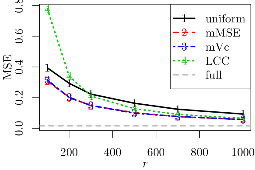
(a) mzNormal

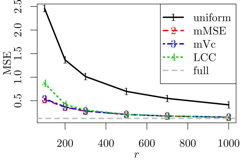
(b) nzNormal

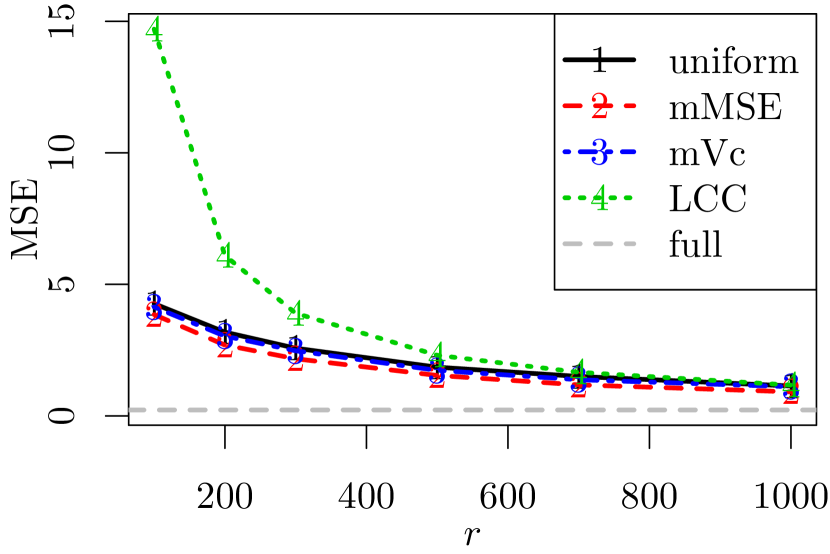
(c) ueNormal

(d) mixNormal

(e) $T_{3}$

(f) EXP

Figure 2: MSEs for different second step subsample size ${r}$ with the first step subsample size being fixed at $r_{0}=200$.

To investigate the effect of different sample size allocations between the two steps, we calculate MSEs for various proportions of first step samples with fixed total subsample sizes. Results are given in Figure 3 with total subsample size $r_{0}+r=800$ and $1200$ for the mzNormal data set. It shows that, the performance of a two-step algorithm improves at first by increasing $r_{0}$, but then it becomes less efficient after a certain point as $r_{0}$ gets larger. This is because if $r_{0}$ is too small, the first step estimate is not accurate; if $r_{0}$ is too close to $r$, then the more informative second step subsample would be small. These observations indicate that, empirically, a value around 0.2 is a good choice for $r_{0}/(r_{0}+r)$ in order to have an efficient two-step algorithm. However, finding a systematic way of determining the optimal sample sizes allocation between two steps needs further study. Results for the other five data sets are similar so they are omitted to save space.

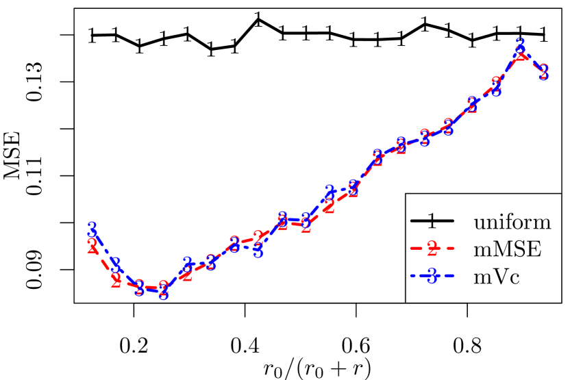
(a) $r_{0}+r=800$

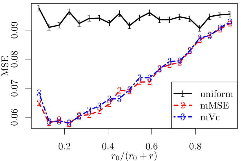
(b) $r_{0}+r=1200$

Figure 3: MSEs vs proportions of the first step subsample with fixed total subsample sizes for the mzNormal data set.

Figure 4 gives proportions of correct classifications on the responses using different methods. To avoid producing over-optimistic results, we generate two full data sets corresponding to each of the six scenarios, use one of them to obtain estimates with different methods, and then perform classification on the other full data. The classification rule is to classify the response to be 1 if $p_{i}(\breve{{\boldsymbol{\beta}}})$ is larger than 0.5, and 0 otherwise. For comparisons, we also use the full data MLE to classify the full data. As shown in Figure 4, all the methods, except LCC with small $r$, produce proportions close to that from using the full data MLE, showing the comparable performance of the OSMAC algorithms to that of the full data approach in classification.

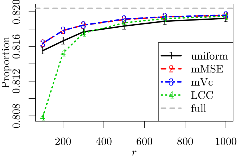
(a) mzNormal

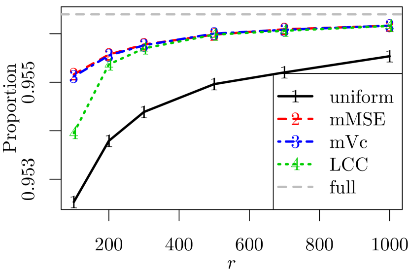
(b) nzNormal

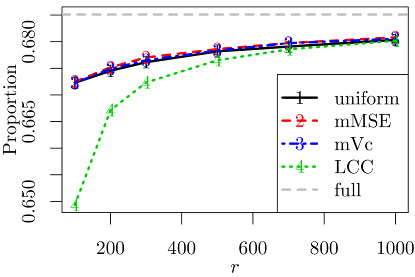
(c) ueNormal

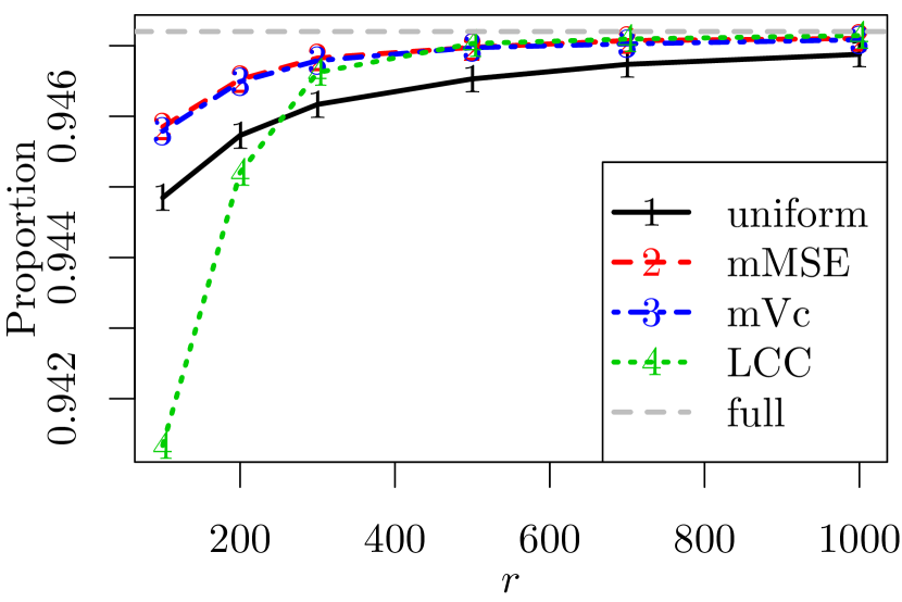
(d) mixNormal

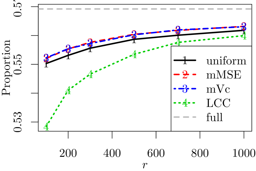
(e) $T_{3}$

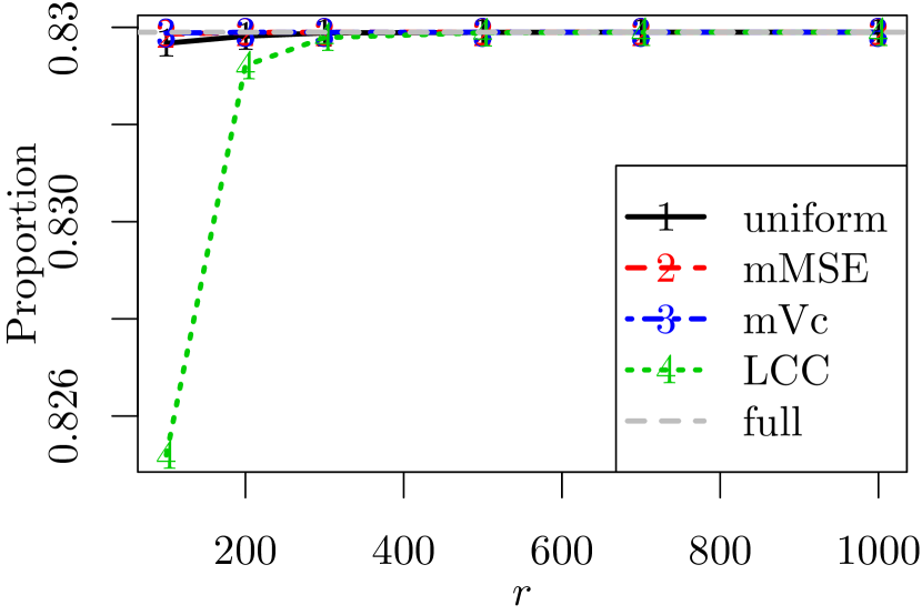
(f) EXP

Figure 4: Proportions of correct classifications for different second step subsample size ${r}$ with the first step subsample size being fixed at $r_{0}=200$. The gray horizontal dashed lines are those using the true parameter.

To assess the performance of the formula in (15), we use it to calculate the estimated MSE, i.e., $\mathrm{tr}(\tilde{{\mathbf{V}}})$, and compare the average estimated MSE with the empirical MSE. Figure 5 presents the results for OSMAC with $\boldsymbol{\pi}^{\mathrm{mMSE}}$. It is seen that the estimated MSEs are very close to the empirical MSEs, except for the case of nzNormal data which is imbalanced. This indicates that the proposed formula works well if the data is not very imbalanced. According to our simulation experiments, it works well if the proportion of 1’s in the responses is between 0.15 and 0.85. For more imbalanced data or rare events data, the formula may not be accurate because the properties of the MLE are different from these for the regular cases (Owen, 2007; King and Zeng, 2001). The performance of the formula in (15) for OSMAC with $\boldsymbol{\pi}^{\mathrm{mVc}}$ is similar to that for OSMAC with $\boldsymbol{\pi}^{\mathrm{mMSE}}$, so results are omitted for clear presentation of the plot.

To further evaluate the performance of the proposed method in statistical inference, we consider confidence interval construction using the asymptotic normality and the estimated variance-covariance matrix in (15). For illustration, we take the parameter of interest as $\beta_{1}$, the first element of ${\boldsymbol{\beta}}$. The corresponding 95% confidence interval is constructed using $\breve{\beta}_{1}\pm Z_{0.975}SE_{\breve{\beta}_{1}}$, where $SE_{\breve{\beta}_{1}}=\sqrt{\breve{V}_{11}}$ is the standard error of $\breve{\beta}_{1}$, and $Z_{0.975}$ is the 97.5th percentile of the standard normal distribution. We repeat the simulation 3000 times and estimate the coverage probability of the confidence interval by the proportion that it covers the true vale of $\beta_{1}$. Figure 6 gives the results. The confidence interval works perfectly for the mxNormal, ueNormal and $T_{3}$ data. For mixNormal and EXP data sets, the empirical coverage probabilities are slightly smaller than the intended confidence level, but the results are acceptable. For the imbalanced nzNormal data, the coverage probabilities are lower than the nominal coverage probabilities. This agrees with the fact in Figure 5 that the formula in (15) does not approximate the asymptotic variance-covariance matrix well for imbalance data.

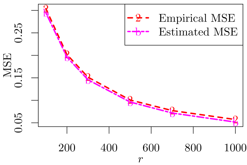
(a) mzNormal

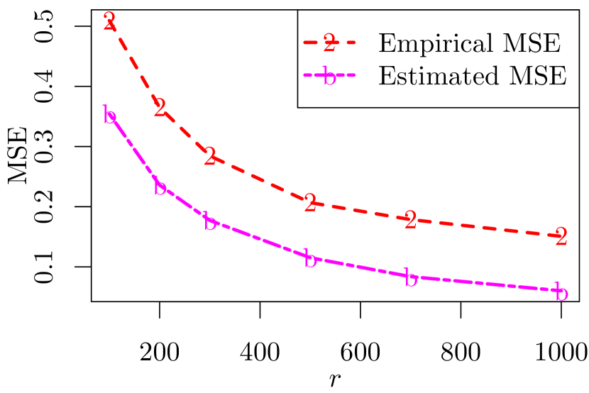
(b) nzNormal

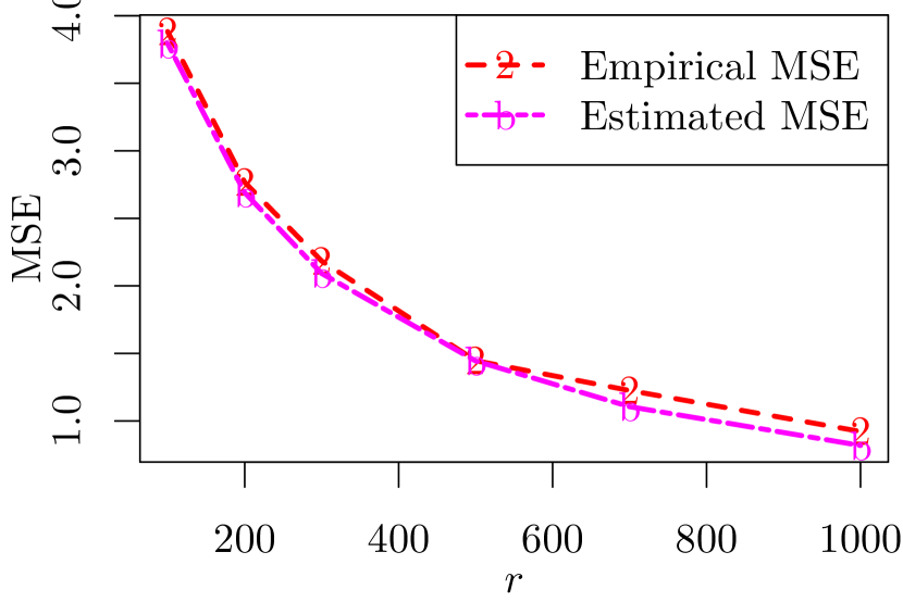
(c) ueNormal

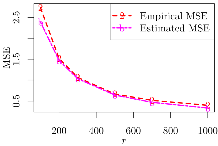
(d) mixNormal

(e) $T_{3}$

(f) EXP

Figure 5: Estimated and empirical MSEs for the OSMAC with $\boldsymbol{\pi}^{\mathrm{mMSE}}$. The first step subsample size is fixed at $r_{0}=200$ and the second step subsample size ${r}$ changes.

(a) mzNormal

(b) nzNormal

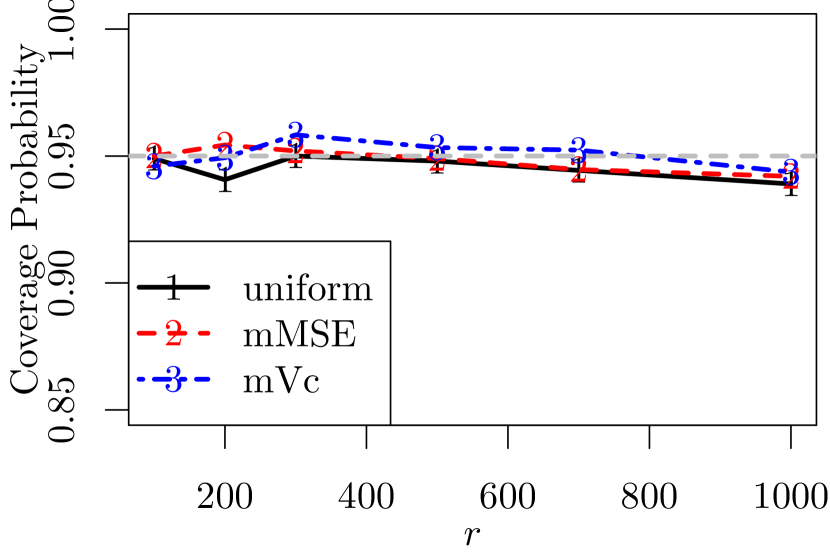
(c) ueNormal

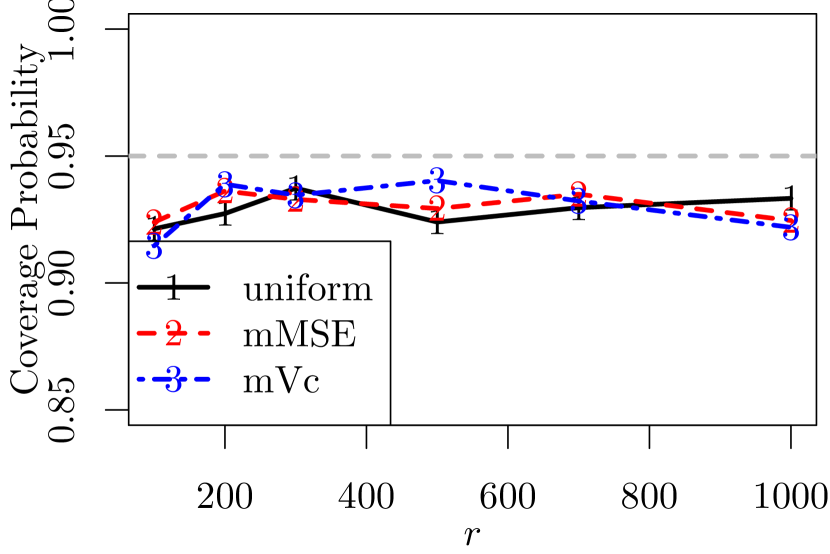
(d) mixNormal

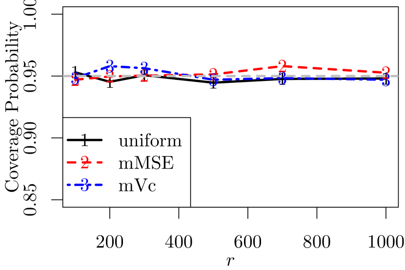
(e) $T_{3}$

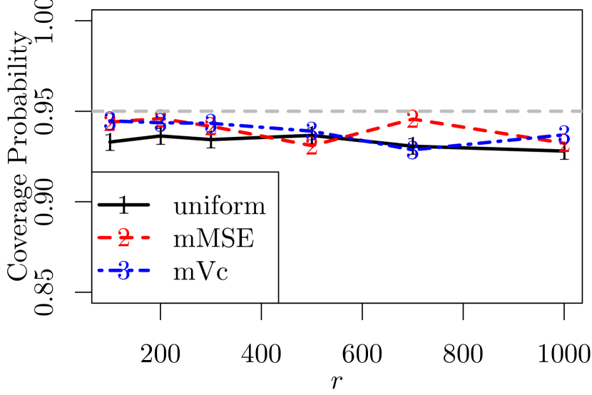
(f) EXP

Figure 6: Empirical coverage probabilities for different second step subsample size r with the first step subsample size being fixed at $r_{0}=200$.

To evaluate the computational efficiency of the subsampling algorithms, we record the computing time and numbers of iterations of Algorithm 2 and the uniform subsampling implemented in the R programming language (R Core Team, 2015). Computations were carried out on a desktop running Window 10 with an Intel I7 processor and 16GB memory. For fair comparison, we counted only the CPU time used by 1000 repetitions of each method. Table 1 gives the results for the mzNormal data set for algorithms based on $\boldsymbol{\pi}^{\mathrm{mMSE}}$, $\boldsymbol{\pi}^{\mathrm{mVc}}$, and $\boldsymbol{\pi}^{\mathrm{UNI}}$. The computing time for using the full data is also given in the last row of Table 1 for comparisons. It is not surprising to observe that the uniform subsampling algorithm requires the least computing time because it does not require an additional step to calculate the SSP. The algorithm based on $\boldsymbol{\pi}^{\mathrm{mMSE}}$ requires longer computing time than the algorithm based on $\boldsymbol{\pi}^{\mathrm{mVc}}$, which agrees with the theoretical analysis in Section 4. All the subsampling algorithms take significantly less computing time compared to using the full data approach. Table 2 presents the average numbers of iterations in Newton’s method. It shows that for Algorithm 2, the first step may require additional iterations compared to the second step, but overall, the required numbers of iterations for all methods are close to 7, the number of iterations used by the full data. This shows that using a smaller subsample does not increase the required number of iterations much for Newton’s method.

Table 1: CPU seconds for the mzNormal data set with $r_{0}=200$ and different ${r}$. The CPU seconds for using the full data is given in the last row.

Method	$r$
	100	200	300	500	700	1000
mMSE	3.340	3.510	3.720	4.100	4.420	4.900
mVc	3.000	3.130	3.330	3.680	4.080	4.580
Uniform	0.690	0.810	0.940	1.190	1.470	1.860
Full data CPU seconds: 13.480

Table 2: Average numbers of iterations used in Newton’s method (3) for the mzNormal data set with $r_{0}=200$ and different ${r}$. For the full data, the number of iterations is 7.

${r}$	mMSE			mVc			uniform
	First step	Second step		First step	Second step
100	7.479	7.288		7.479	7.296		7.378
200	7.479	7.244		7.479	7.241		7.305
300	7.482	7.230		7.482	7.214		7.259
500	7.458	7.200		7.458	7.185		7.174
700	7.472	7.190		7.472	7.180		7.136
1000	7.471	7.181		7.471	7.158		7.091

To further investigate the computational gain of the subsampling approach for massive data volume, we increase the value of $d$ to $d=50$ and increase the values of $n$ to be $n=10^{4},10^{5},10^{6}$ and $10^{7}$. We record the computing time for the case when ${\mathbf{x}}$ is multivariate normal. Table 3 presents the result based on one iteration of calculation. It is seen that as $n$ increases, the computational efficiency for a subsampling method relative to the full data approach is getting more and more significant.

Table 3: CPU seconds with $r_{0}=200$, ${r}=1000$ and different full data size $n$ when the covariates are from a $d=50$ dimensional normal distribution.

Method	$n$
	$10^{4}$	$10^{5}$	$10^{6}$	$10^{7}$
mMSE	0.050	0.270	3.290	37.730
mVc	0.030	0.070	0.520	6.640
Uniform	0.010	0.030	0.020	0.830
Full	0.150	1.710	16.530	310.450

5.1.1 Numerical evaluations for rare events data

To investigate the performance of the proposed method for the case of rare events, we generate rare events data using the same configurations that are used to generate the nzNormal data, except that we change the mean of ${\mathbf{x}}$ to -2.14 or -2.9. With these values, 1.01% and 0.14% of responses are 1 in the full data of size $n=10000$.

Figure 7 presents the results for these two scenarios. It is seen that both mMSE and mVc work well for these two scenarios and their performances are similar. The uniform subsampling is neither stable nor efficient. When the event rate is 0.14%, corresponding to the subsample sizes of 300, 400, 500, 700, 900, and 1200, there are 903, 848, 801, 711, 615, and 491 cases out of 1000 repetitions of the simulation that the MLE are not found. For the cases that the MLE are found, the MSEs are 78.27907, 23.28546, 34.16891, 42.43081, 26.38999, and 19.25178, respectively. These MSEs are much larger than those from the OSMAC and thus are omitted in Figure 7 for better presentation. For the OSMAC, there are 8 cases out of 1000 that the MLE are not found only when $r_{0}=200$ and $r=100$.

For comparison, we also calculate the MSE of the full data approach using 1000 Bootstrap samples (the gray dashed line). Note that the Bootstrap is the uniform subsampling with the subsample size being equal to the full data sample size. Interestingly, it is seen from Figure 7 that OSMAC methods can produce MSEs that are much smaller than the Bootstrap MSEs. To further investigate this interesting case, we carry out another simulation using the exact same setup. A full data is generated in each repetition and hence the resultant MSEs are the unconditional MSEs. Results are presented in Figure 8. Although the unconditional MSEs of the OSMAC methods are larger than that of the full data approach, they are very close when $r$ gets large, especially when the rare event rate is $0.11\%$. Here, $0.11\%$ is the average percentage of 1’s in the responses of all 1000 simulated full data. Note that the true value of ${\boldsymbol{\beta}}$ is used in calculating both the conditional MSEs and the unconditional MSEs. Comparing Figure 7 (b) and Figure 8 (b), conditional inference of OSMAC can indeed be more efficient than the full data approach for rare events data. These two figures also indicate that the original Bootstrap method does not work perfectly for the case of rare events data. For additional results on more extreme rare events data, please read Section S.2.1 in the Supplementary Material.

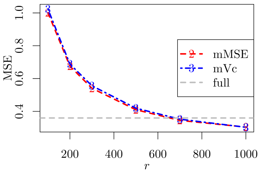
(a) 1.01% of $y_{i}$’s are 1

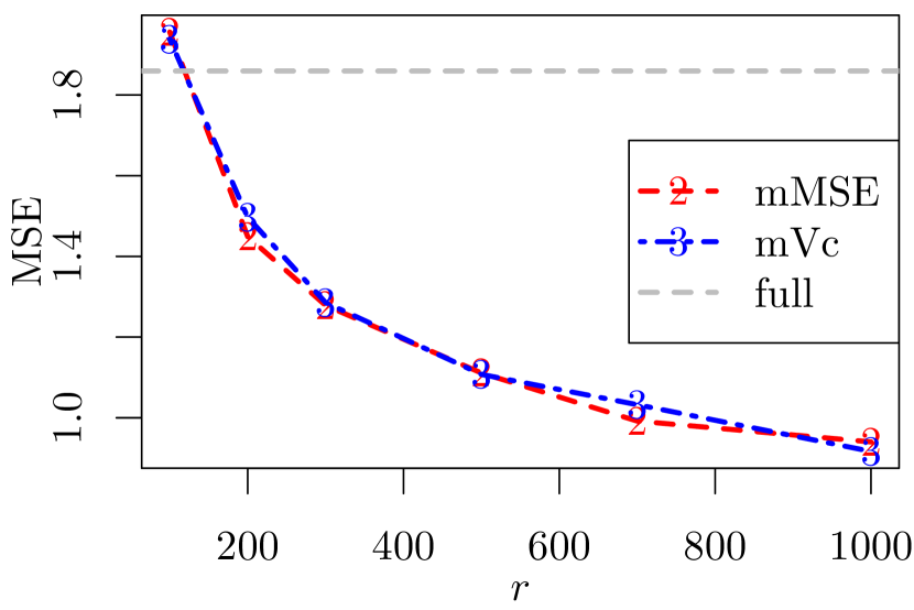
(b) 0.14% of $y_{i}$’s are 1

Figure 7: MSEs for rare event data with different second step subsample size $r$ and a fixed first step subsample size $r_{0}=200$, where the covariates follow multivariate normal distributions.

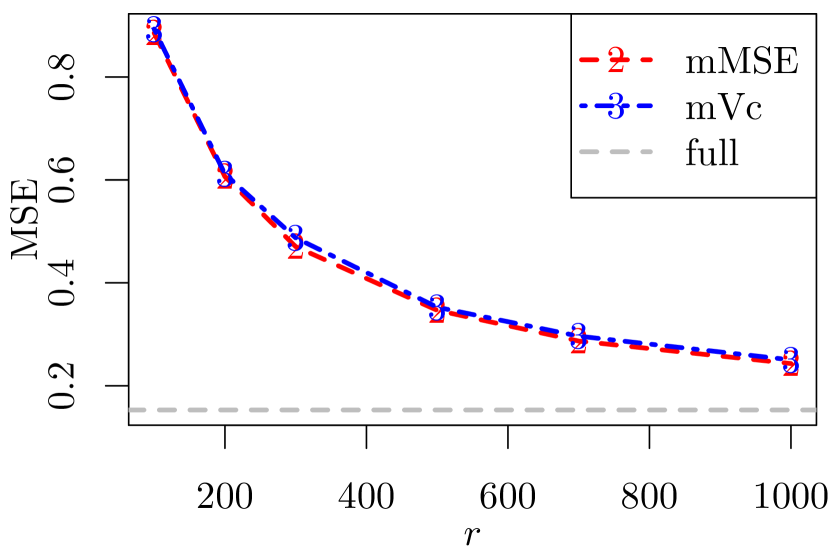
(a) 1.04% of $y_{i}$’s are 1

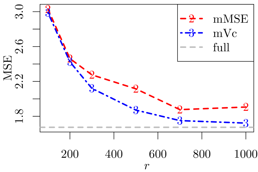
(b) 0.11% of $y_{i}$’s are 1

Figure 8: Unconditional MSEs for rare event data with different second step subsample size $r$ and a fixed first step subsample size $r_{0}=200$, where the covariates follow multivariate normal distributions.

5.2 Census income data set

In this section, we apply the proposed methods to a census income data set (Kohavi, 1996), which was extracted from the 1994 Census database. There are totally $48,842$ observations in this data set, and the response variable is whether a person’s income exceeds $50K a year. There are 11,687 individuals (23.93%) in the data whose income exceed $50K a year. Inferential task is to estimate the effect on income from the following covariates: $x_{1}$, age; $x_{2}$, final weight (Fnlwgt); $x_{3}$, highest level of education in numerical form; $x_{4}$, capital loss (LosCap); $x_{5}$, hours worked per week. The variable final weight ($x_{2}$) is the number of people the observation represents. The values were assigned by Population Division at the Census Bureau, and they are related to the socio-economic characteristic, i.e., people with similar socio-economic characteristics have similar weights. Capital loss ($x_{5}$) is the loss in income due to bad investments; it is the difference between lower selling prices of investments and higher purchasing prices of investments made by the individual.

The parameter corresponding to $x_{i}$ is denoted as $\beta_{i}$ for $i=1,...,5$. An intercept parameter, say $\beta_{0}$, is also include in the model. Another interest is to determine whether a person’s income exceeds $50K a year using the covariates. We obtained the data from the Machine Learning Repository (Lichman, 2013), where it is partitioned into a training set of $n=32,561$ observations and a validation set of $16,281$ observations. Thus we apply the proposed method on the train set and use the validation set to evaluate the performance of classification.

For this data set, the full data estimates using all the observation in the training set are: $\hat{\beta}_{0}=-8.637$ (0.116), $\hat{\beta}_{1}=0.637$ (0.016), $\hat{\beta}_{2}=0.065$ (0.015), $\hat{\beta}_{3}=0.878$ (0.017), $\hat{\beta}_{4}=0.234$ (0.013) and $\hat{\beta}_{5}=0.525$ (0.016), where the numbers in the parentheses are the associated standard errors. Table 4 gives the average of parameter estimates along with the empirical and estimated standard errors from different methods based on 1000 subsamples of $r_{0}+r=1200$ with $r_{0}=200$ and ${r}=1000$. It is seen that all subsampling method produce estimates close to those from the full data approach. In general, OSMAC with $\boldsymbol{\pi}^{\mathrm{mMSE}}$ and OSMAC with $\boldsymbol{\pi}^{\mathrm{mVc}}$ produce the smallest standard errors. The estimated standard errors are very close to the empirical standard errors, showing that the proposed asymptotic variance-covariance formula in (15) works well for the read data. The standard errors for the subsample estimates are larger than those for the full data estimates. However, they are quite good in view of the relatively small subsample size. All methods show that the effect of each variable on income is positive. However, the effect of final weight is not significant at significance level 0.05 according to any subsample-based method, while this variable is significant at the same significance level according to the full data analysis. The reason is that the subsample inference is not as powerful as the full data approach due to its relatively smaller sample size. Actually, for statistical inference in large sample, no matter how small the true parameter is, as long as it is a nonzero constant, the corresponding variable can always be detected as significant with large enough sample size. This is also true for conditional inference based on a subsample if the subsample size is large enough. It is interesting that capital loss has a significantly positive effect on income, this is because people with low income seldom have investments.

Table 4: Average estimates for the Adult income data set based on 1000 subsamples. The numbers in the parentheses are the associated empirical and average estimated standard errors, respectively. In the table, $\beta_{1}$ is for age, $\beta_{2}$ is for final weight, $\beta_{3}$ is for highest level of education in numerical form, $\beta_{4}$ is for capital loss, and $\beta_{5}$ is for hours worked per week.

	uniform	mMSE	mVc
Intercept	-8.686 (0.629, 0.609)	-8.660 (0.430, 0.428)	-8.639 (0.513, 0.510)
$\beta_{1}$	0.638 (0.079, 0.078)	0.640 (0.068, 0.071)	0.640 (0.068, 0.067)
$\beta_{2}$	0.061 (0.076, 0.077)	0.065 (0.067, 0.068)	0.063 (0.061, 0.062)
$\beta_{3}$	0.882 (0.090, 0.090)	0.881 (0.079, 0.075)	0.878 (0.072, 0.072)
$\beta_{4}$	0.232 (0.070, 0.071)	0.231 (0.058, 0.059)	0.232 (0.060, 0.057)
$\beta_{5}$	0.533 (0.085, 0.087)	0.526 (0.068, 0.070)	0.526 (0.071, 0.070)

Figure 9 (a) shows the MSEs that were calculated from $S=1000$ subsamples of size $r_{0}+r$ with a fixed $r_{0}=200$. In this figure, all MSEs are small and go to 0 as the subsample size gets large, showing the estimation consistency of the subsampling methods. The OSMAC with $\boldsymbol{\pi}^{\mathrm{mMSE}}$ always has the smallest MSE. Figure 9 (b) gives the proportions of correct classifications on the responses in the validation set for different second step subsample sizes with a fixed $r_{0}=200$ when the classification threshold is 0.5. For comparison, we also obtained the results of classification using the full data estimate which is the gray horizontal dashed line. Indeed, using all the $n=32,561$ observations in the training set yields better results than using subsamples of much smaller sizes, but the difference is really small. One point worth to mention is that although the OSMAC with $\boldsymbol{\pi}^{\mathrm{mMSE}}$ always yields a smaller MSE compared to the OSMAC with $\boldsymbol{\pi}^{\mathrm{mVc}}$, its performance in classification is inferior to the OSMAC with $\boldsymbol{\pi}^{\mathrm{mVc}}$. This is because $\boldsymbol{\pi}^{\mathrm{mMSE}}$ aims to minimize the asymptotic MSE and may not minimize the misclassification rate, although the two goals are highly related.

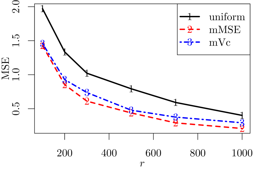
(a) MSEs vs ${r}$

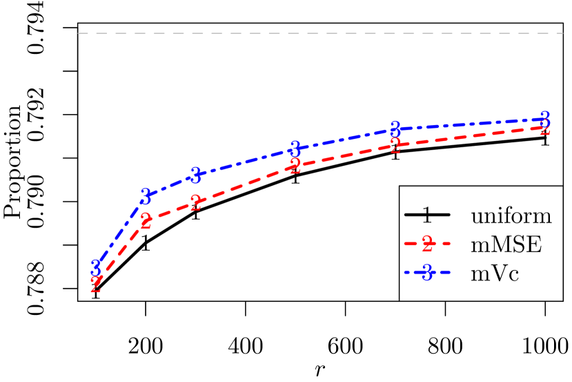
(b) Proportions of correct classifications vs $r$

Figure 9: MSEs and proportions of correct classifications for the adult income data set with $r_{0}=200$ and different second step subsample size ${r}$. The gray horizontal dashed line in figure (b) is the result using the full data MLE.

5.3 Supersymmetric benchmark data set

We apply the subsampling methods to a supersymmetric (SUSY) benchmark data set (Baldi et al., 2014) in this section. The data set is available from the Machine Learning Repository (Lichman, 2013) at this link: https://archive.ics.uci.edu/ml/datasets/SUSY. The goal is to distinguish between a process where new supersymmetric particles are produced and a background process, utilizing the 18 kinematic features in the data set. The full sample size is $5,000,000$ and the data file is about 2.4 gigabytes. About 54.24% of the responses in the full data are from the background process. We use the first $n=4,500,000$ observation as the training set and use the last $500,000$ observations as the validation set.

Figures 10 gives the MSEs and proportions of correct classification when the classification probability threshold is 0.5. It is seen that the OSMAC with $\boldsymbol{\pi}^{\mathrm{mMSE}}$ always results in the smallest MSEs. For classifications, the result from the full data is better than the subsampling methods, but the difference is not significant. Among the three subsampling methods, the OSMAC with $\boldsymbol{\pi}^{\mathrm{mVc}}$ has the best performance in classification.

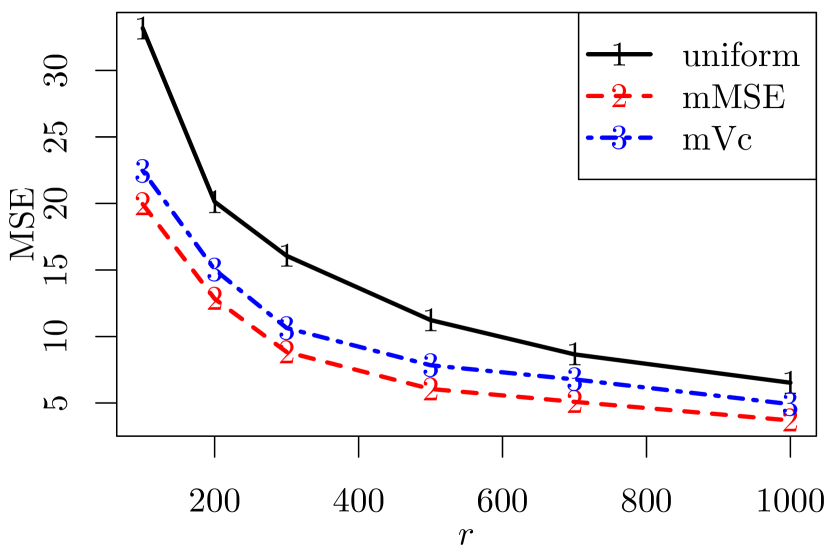
(a) MSEs vs ${r}$

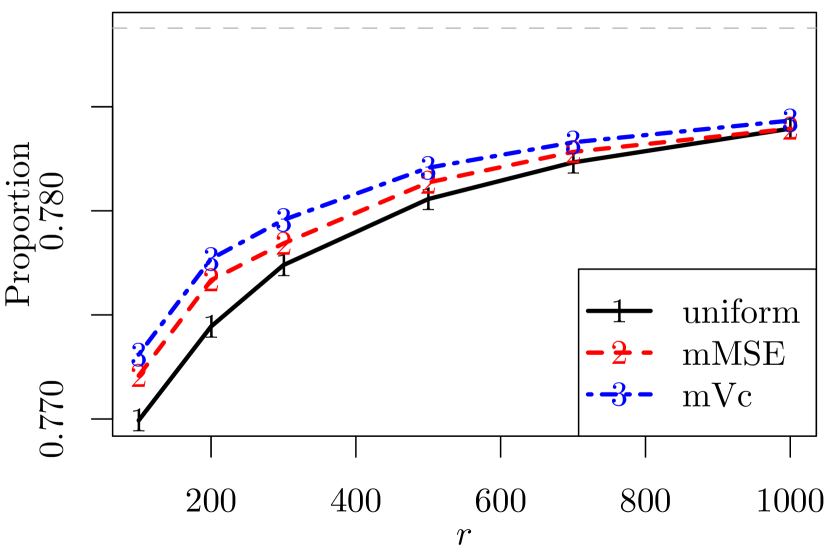
(b) Proportions of correct classifications vs $r$

Figure 10: MSEs and proportions of correct classifications for for the SUSY data set with $r_{0}=200$ and different second step subsample size ${r}$. The gray horizontal dashed line in figure (b) is the result using the full data MLE.

To further evaluate the performance of the OSMAC methods as classifiers, we create receiver operating characteristic (ROC) curves using classification probability thresholds between 0 and 1, and then calculate the areas under the ROC curves (AUC). As pointed out by an Associate Editor, the theoretical investigation of this paper focus on parameter estimation, and classification is not theoretically studied. These two goals, although being different, are highly connected. Since logistic regression models are commonly used for classification, the relevant performance is also important for practical application. Table 5 presents the results based on 1000 subsamples of size $r_{0}+r=1000$ from the full data. For the two step algorithm, $r_{0}=200$ and ${r}=800$. All the AUCs are around 0.85, meaning that the classifiers all have good performance.

For the same data set considered here, the deep learning method (DL) in Baldi et al. (2014) produced an AUC of 0.88 while the AUCs from the OSMAC approach with different SSPs are around 0.85. However the DL used the full data set and had to optimize a much more complicated model (“a five-layer neural network with 300 hidden units in each layer” (Baldi et al., 2014)), while OSMAC just used $r=1000$ observations and the target function to optimize is the log-likelihood function of a logistic regression model. Due to computational costs, the optimization in Baldi et al. (2014) included “combinations of the pre-training methods, network architectures, initial learning rates, and regularization methods.” For the OSMAC, the optimization was done by using a standard Newton’s method directly. The computations of Baldi et al. (2014) “were performed using machines with 16 Intel Xeon cores, an NVIDIA Tesla C2070 graphics processor, and 64 GB memory. All neural networks were trained using the GPU-accelerated Theano and Pylearn2 software libraries”. Our analysis was just carried out on a normal PC with an Intel I7 processor and 16GB memory. Clearly, Baldi et al. (2014)’s method requires special computing resources and coding skills, but anyone with basic programming ability is able to implement the OSMAC. Due to the special requirements of Baldi et al. (2014)’s method, we are not able to replicate their results and thus cannot report the computing time. For our OSMAC with $\boldsymbol{\pi}^{\mathrm{mMSE}}$ and $\boldsymbol{\pi}^{\mathrm{mVc}}$, the average CPU seconds to obtain parameter estimates are 3.400 and 1.079 seconds, respectively. The full data MLE takes an average of 24.060 seconds to run.

Table 5: Average AUC (as percentage) for the SUSY data set based on 1000 subsamples. A number in the parentheses is the associated standard error (as percentage) of the 1000 AUCs.

Method		AUC % (SE)
uniform		85.06 (0.29)
mMSE		85.08 (0.30)
mVc		85.17 (0.25)
Full		85.75

6 Discussion

In this paper, we proposed the OSMAC approach for logistic regression in order to overcome the computation bottleneck resulted from the explosive growth of data volume. Not only were theoretical statistical asymptotic results derived, but also optimal subsampling methods were given. Furthermore, we developeded a two-step subsampling algorithm to approximate optimal subsampling strategies and proved that the resultant estimator is consistent and asymptotically normal with the optimal variance-covariance matrix. As shown in our numerical experiments, the OSMAC approach for logistic regression is a computationally feasible method for super-large samples, and it yields a good approximation to the results based on full data. There are important issues in this paper that we will investigate in the future.

1. In our numerical experiments, the formula in (15) underestimates the asymptotic variance-covariance matrix and thus does not produce an accurate approximation for rare events data. It is unclear whether the technique in King and Zeng (2001) can be applied to develop an improved estimator of the asymptotic variance-covariance matrix in the case of rare event. It is an interesting question worth further investigations.

2. We have chosen to minimize the trace of ${\mathbf{V}}$ or ${\mathbf{V}}_{c}$ to define optimal subsampling algorithms. The idea is from the $A$-optimality criterion in the theory of optimal experimental designs (Kiefer, 1959). There are other optimality criteria emphasizing different inferential purposes, such as the $C$-optimality and the $D$-optimality. How to use these optimality criteria to develop high quality algorithms is undoubtedly a topic worthy of future study.

Supplementary Material
for “Optimal Subsampling for Large Sample Logistic Regression”

S.1 Proofs

In this section we prove the theorems in the paper.

S.1.1 Proof of Theorem 1

We begin by establishing a lemma that will be used in the proof of Theorems 1 and 2.

Lemma 1.

If Assumptions 1 and 2 hold, then conditionally on ${\mathcal{F}_{n}}$ in probability,

$$\tilde{{\mathbf{M}}}_{X}-{\mathbf{M}}_{X} =O_{P|{\mathcal{F}_{n}}}(r^{-1/2}),$$ (S.1)

$$\frac{1}{n}\frac{\partial\ell^{*}(\hat{{\boldsymbol{\beta}}}_{{{\textnormal{\tiny MLE}}}})}{\partial{\boldsymbol{\beta}}} =O_{P|{\mathcal{F}_{n}}}(r^{-1/2}),$$ (S.2)

where

$$\tilde{{\mathbf{M}}}_{X}=\frac{1}{n}\frac{\partial^{2}\ell^{*}(\hat{{\boldsymbol{\beta}}}_{{{\textnormal{\tiny MLE}}}})}{\partial{\boldsymbol{\beta}}\partial{\boldsymbol{\beta}}^{T}}=\frac{1}{nr}\sum_{i=1}^{r}\frac{w_{i}^{*}(\hat{{\boldsymbol{\beta}}}_{{{\textnormal{\tiny MLE}}}}){\mathbf{x}}_{i}^{*}({\mathbf{x}}_{i}^{*})^{T}}{\pi^{*}_{i}}.$$

Proof.

Direct calculation yields

$${\mathrm{E}}(\tilde{{\mathbf{M}}}_{X}|{\mathcal{F}_{n}})={\mathbf{M}}_{X}.$$ (S.3)

For any component $\tilde{{\mathbf{M}}}_{X}^{j_{1}j_{2}}$ of $\tilde{{\mathbf{M}}}_{X}$ where $1\leq j_{1},j_{2}\leq d$,

$${\mathrm{Var}}\left(\frac{1}{n}\tilde{{\mathbf{M}}}_{X}^{j_{1}j_{2}}\Big{|}{\mathcal{F}_{n}}\right)= \frac{1}{r}\sum_{i=1}^{n}\pi_{i}\left\{\frac{w_{i}(\hat{{\boldsymbol{\beta}}}_{{{\textnormal{\tiny MLE}}}})x_{ij_{1}}x_{ij_{2}}}{n\pi_{i}}-{\mathbf{M}}_{X}^{j_{1}j_{2}}\right\}^{2}$$

$$= \frac{1}{rn^{2}}\sum_{i=1}^{n}\frac{w_{i}(\hat{{\boldsymbol{\beta}}}_{{{\textnormal{\tiny MLE}}}})^{2}(x_{ij_{1}}x_{ij_{2}}^{T})^{2}}{\pi_{i}}-\frac{1}{r}({\mathbf{M}}_{X}^{j_{1}j_{2}})^{2}$$

$$\leq \frac{1}{16rn^{2}}\sum_{i=1}^{n}\frac{\|{\mathbf{x}}_{i}\|^{4}}{\pi_{i}}-\frac{1}{r}({\mathbf{M}}_{X}^{j_{1}j_{2}})^{2}$$

$$= O_{P}(r^{-1}),$$

where the second last inequality holds by the fact that $0<w_{i}(\hat{{\boldsymbol{\beta}}}_{{{\textnormal{\tiny MLE}}}})\leq 1/4$ and the last equality is from Assumption 2. Using Markov’s inequality, this result and (S.3), implies (S.1).

To prove (S.2), direct calculation yields,

$${\mathrm{E}}\left\{\frac{1}{n}\frac{\partial\ell^{*}(\hat{{\boldsymbol{\beta}}}_{{{\textnormal{\tiny MLE}}}})}{\partial{\boldsymbol{\beta}}}\bigg{|}{\mathcal{F}_{n}}\right\}=\frac{1}{nr}\frac{\partial\ell^{*}(\hat{{\boldsymbol{\beta}}}_{{{\textnormal{\tiny MLE}}}})}{\partial{\boldsymbol{\beta}}}=0.$$ (S.4)

From Assumption 2,

$${\mathrm{Var}}\left\{\frac{1}{n}\frac{\partial\ell^{*}(\hat{{\boldsymbol{\beta}}}_{{{\textnormal{\tiny MLE}}}})}{\partial{\boldsymbol{\beta}}}\bigg{|}{\mathcal{F}_{n}}\right\}=\frac{1}{n^{2}r}\sum_{i=1}^{n}\frac{\{y_{i}-p_{i}(\hat{{\boldsymbol{\beta}}}_{{{\textnormal{\tiny MLE}}}})\}^{2}{\mathbf{x}}_{i}{\mathbf{x}}_{i}^{T}}{\pi_{i}}\leq\frac{1}{n^{2}r}\sum_{i=1}^{n}\frac{{\mathbf{x}}_{i}{\mathbf{x}}_{i}^{T}}{\pi_{i}}=O_{P}(r^{-1}).$$ (S.5)

From (S.4), (S.5) and Markov’s inequality, (S.2) follows. ∎

Now we prove Theorem 1. Note that $t_{i}({\boldsymbol{\beta}})=y_{i}\log p_{i}({\boldsymbol{\beta}})+(1-y_{i})\log\{1-p_{i}({\boldsymbol{\beta}})\}$, $t_{i}^{*}({\boldsymbol{\beta}})=y_{i}^{*}\log p_{i}^{*}({\boldsymbol{\beta}})+(1-y_{i}^{*})\log\{1-p_{i}^{*}({\boldsymbol{\beta}})\}$,

$$\ell^{*}({\boldsymbol{\beta}})=\frac{1}{r}\sum_{i=1}^{r}\frac{t_{i}^{*}({\boldsymbol{\beta}})}{\pi_{i}^{*}},\ \ \text{and}\ \ \ell({\boldsymbol{\beta}})=\sum_{i=1}^{n}t_{i}({\boldsymbol{\beta}}).$$

By direct calculation under the conditional distribution of subsample given ${\mathcal{F}_{n}}$,

$${\mathrm{E}}\left\{\frac{\ell^{*}({\boldsymbol{\beta}})}{n}-\frac{\ell({\boldsymbol{\beta}})}{n}\bigg{|}{\mathcal{F}_{n}}\right\}^{2}=\frac{1}{r}\left[\frac{1}{n^{2}}\sum_{i=1}^{n}\frac{t_{i}^{2}({\boldsymbol{\beta}})}{\pi_{i}}-\left(\frac{1}{n}\sum_{i=1}^{n}t_{i}({\boldsymbol{\beta}})\right)^{2}\right].$$ (S.6)

Note that $|t_{i}({\boldsymbol{\beta}})|\leq\log 4+2\|{\mathbf{x}}_{i}\|\|{\boldsymbol{\beta}}\|$. Therefore, from Assumption 1,

$$\frac{1}{n^{2}}\sum_{i=1}^{n}\frac{t_{i}^{2}({\boldsymbol{\beta}})}{\pi_{i}}-\left(\frac{1}{n}\sum_{i=1}^{n}t_{i}({\boldsymbol{\beta}})\right)^{2}\leq \frac{1}{n^{2}}\sum_{i=1}^{n}\frac{t_{i}^{2}({\boldsymbol{\beta}})}{\pi_{i}}+\left(\frac{1}{n}\sum_{i=1}^{n}|t_{i}({\boldsymbol{\beta}})|\right)^{2}=O_{P}(1).$$ (S.7)

Therefore combing (S.6) and (S.7), $n^{-1}\ell^{*}({\boldsymbol{\beta}})-n^{-1}\ell({\boldsymbol{\beta}})\rightarrow 0$ in conditional probability given ${\mathcal{F}_{n}}$. Note that the parameter space is compact and $\hat{{\boldsymbol{\beta}}}_{{{\textnormal{\tiny MLE}}}}$ is the unique global maximum of the continuous convex function $\ell({\boldsymbol{\beta}})$. Thus, from Theorem 5.9 and its remark of van der Vaart (1998), conditionally on ${\mathcal{F}_{n}}$ in probability,

$$\|\tilde{{\boldsymbol{\beta}}}-\hat{{\boldsymbol{\beta}}}_{{{\textnormal{\tiny MLE}}}}\|=o_{P|{\mathcal{F}_{n}}}(1)$$ (S.8)

The consistency proved above ensures that $\tilde{{\boldsymbol{\beta}}}$ is close to $\hat{{\boldsymbol{\beta}}}_{{{\textnormal{\tiny MLE}}}}$ as long as $r$ is not small. Using Taylor’s theorem (c.f. Chapter 4 of Ferguson, 1996),

$$0=\frac{\dot{\ell}^{*}_{j}(\tilde{{\boldsymbol{\beta}}})}{n}= \frac{\dot{\ell}^{*}_{j}(\hat{{\boldsymbol{\beta}}}_{{{\textnormal{\tiny MLE}}}})}{n}+\frac{1}{n}\frac{\partial\dot{\ell}^{*}_{j}(\hat{{\boldsymbol{\beta}}}_{{{\textnormal{\tiny MLE}}}})}{\partial{\boldsymbol{\beta}}^{T}}(\tilde{{\boldsymbol{\beta}}}-\hat{{\boldsymbol{\beta}}}_{{{\textnormal{\tiny MLE}}}})+\frac{1}{n}R_{j}$$ (S.9)

where $\dot{\ell}^{*}_{j}({{\boldsymbol{\beta}}})$ is the partial derivative of $\ell^{*}({{\boldsymbol{\beta}}})$ with respect to $\beta_{j}$, and

$$R_{j}=(\tilde{{\boldsymbol{\beta}}}-\hat{{\boldsymbol{\beta}}}_{{{\textnormal{\tiny MLE}}}})^{T}\int_{0}^{1}\int_{0}^{1}\frac{\partial^{2}\dot{\ell}^{*}_{j}\{\hat{{\boldsymbol{\beta}}}_{{{\textnormal{\tiny MLE}}}}+uv(\tilde{{\boldsymbol{\beta}}}-\hat{{\boldsymbol{\beta}}}_{{{\textnormal{\tiny MLE}}}})\}}{\partial{\boldsymbol{\beta}}\partial{\boldsymbol{\beta}}^{T}}v{\mathrm{d}}u{\mathrm{d}}v\ (\tilde{{\boldsymbol{\beta}}}-\hat{{\boldsymbol{\beta}}}_{{{\textnormal{\tiny MLE}}}}).$$

Note that

$$\left\|\frac{\partial^{2}\dot{\ell}^{*}_{j}({\boldsymbol{\beta}})}{\partial{\boldsymbol{\beta}}\partial{\boldsymbol{\beta}}^{T}}\right\|= \frac{1}{r}\left\|\sum_{i=1}^{r}\frac{p^{*}_{i}({\boldsymbol{\beta}})\{1-p^{*}_{i}({\boldsymbol{\beta}})\}\{1-2p^{*}_{i}({\boldsymbol{\beta}})\}}{\pi^{*}_{i}}x^{*}_{ij}{\mathbf{x}}^{*}_{i}{{\mathbf{x}}^{*}_{i}}^{T}\right\|\leq\frac{1}{r}\sum_{i=1}^{r}\frac{\|{\mathbf{x}}^{*}_{i}\|^{3}}{\pi^{*}_{i}}$$

for all ${\boldsymbol{\beta}}$. Thus

$$\left\|\int_{0}^{1}\int_{0}^{1}\frac{\partial^{2}\dot{\ell}^{*}_{j}\{\hat{{\boldsymbol{\beta}}}_{{{\textnormal{\tiny MLE}}}}+uv(\tilde{{\boldsymbol{\beta}}}-\hat{{\boldsymbol{\beta}}}_{{{\textnormal{\tiny MLE}}}})\}}{\partial{\boldsymbol{\beta}}\partial{\boldsymbol{\beta}}^{T}}v{\mathrm{d}}u{\mathrm{d}}v\ \right\|\leq\frac{1}{2r}\sum_{i=1}^{r}\frac{\|{\mathbf{x}}^{*}_{i}\|^{3}}{\pi^{*}_{i}}=O_{P|{\mathcal{F}_{n}}}(n),$$ (S.10)

where the last equality is from the fact that

$$P\left(\frac{1}{nr}\sum_{i=1}^{r}\frac{\|{\mathbf{x}}^{*}_{i}\|^{3}}{\pi^{*}_{i}}\geq\tau\Bigg{|}{\mathcal{F}_{n}}\right)\leq\frac{1}{nr\tau}\sum_{i=1}^{r}{\mathrm{E}}\left(\frac{\|{\mathbf{x}}^{*}_{i}\|^{3}}{\pi^{*}_{i}}\Bigg{|}{\mathcal{F}_{n}}\right)=\frac{1}{n\tau}\sum_{i=1}^{n}\|{\mathbf{x}}_{i}\|^{3}\rightarrow 0,$$ (S.11)

in probability as $\tau\rightarrow\infty$ by Assumption 2. From (S.9) and (S.10),

$$\tilde{{\boldsymbol{\beta}}}-\hat{{\boldsymbol{\beta}}}_{{{\textnormal{\tiny MLE}}}}=-\tilde{{\mathbf{M}}}_{X}^{-1}\left\{\frac{\dot{\ell}^{*}(\hat{{\boldsymbol{\beta}}}_{{{\textnormal{\tiny MLE}}}})}{n}+O_{P|{\mathcal{F}_{n}}}(\|\tilde{{\boldsymbol{\beta}}}-\hat{{\boldsymbol{\beta}}}_{{{\textnormal{\tiny MLE}}}}\|^{2})\right\}.$$ (S.12)

From (S.1) of Lemma 1, $\tilde{{\mathbf{M}}}_{X}^{-1}=O_{P|{\mathcal{F}_{n}}}(1)$. Combining this with (S.2), (S.8) and (S.12)

$$\tilde{{\boldsymbol{\beta}}}-\hat{{\boldsymbol{\beta}}}_{{{\textnormal{\tiny MLE}}}}=O_{P|{\mathcal{F}_{n}}}(r^{-1/2})+o_{P|{\mathcal{F}_{n}}}(\|\tilde{{\boldsymbol{\beta}}}-\hat{{\boldsymbol{\beta}}}_{{{\textnormal{\tiny MLE}}}}\|),$$

which implies that

$$\tilde{{\boldsymbol{\beta}}}-\hat{{\boldsymbol{\beta}}}_{{{\textnormal{\tiny MLE}}}}=O_{P|{\mathcal{F}_{n}}}(r^{-1/2}).$$ (S.13)

S.1.2 Proof of Theorem 2

Note that

$$\frac{\dot{\ell}^{*}(\hat{{\boldsymbol{\beta}}}_{{{\textnormal{\tiny MLE}}}})}{n}=\frac{1}{r}\sum_{i=1}^{r}\frac{\{y^{*}_{i}-p^{*}_{i}(\hat{{\boldsymbol{\beta}}}_{{{\textnormal{\tiny MLE}}}})\}{\mathbf{x}}^{*}_{i}}{n\pi^{*}_{i}}\equiv\frac{1}{r}\sum_{i=1}^{r}{\boldsymbol{\eta}}_{i}$$ (S.14)

Given ${\mathcal{F}_{n}}$, ${\boldsymbol{\eta}}_{1},...,{\boldsymbol{\eta}}_{r}$ are i.i.d, with mean $\mathbf{0}$ and variance,

$${\mathrm{Var}}({\boldsymbol{\eta}}_{i}|{\mathcal{F}_{n}})=r{\mathbf{V}}_{c}=\frac{1}{n^{2}}\sum_{i=1}^{n}\frac{\{y_{i}-p_{i}(\hat{{\boldsymbol{\beta}}}_{{{\textnormal{\tiny MLE}}}})\}^{2}{\mathbf{x}}_{i}{\mathbf{x}}_{i}^{T}}{\pi_{i}}=O_{P}(1).$$ (S.15)

Meanwhile, for every $\varepsilon>0$ and some $\delta>0$,

$$\sum_{i=1}^{r}{\mathrm{E}}\{\|r^{-1/2}{\boldsymbol{\eta}}_{i}\|^{2}I(\|{\boldsymbol{\eta}}_{i}\|>r^{1/2}\varepsilon)|{\mathcal{F}_{n}}\}$$

$$\leq\frac{1}{r^{1+\delta/2}\varepsilon^{\delta}}\sum_{i=1}^{r}{\mathrm{E}}\{\|{\boldsymbol{\eta}}_{i}\|^{2+\delta}I(\|{\boldsymbol{\eta}}_{i}\|>r^{1/2}\varepsilon)|{\mathcal{F}_{n}}\}$$

$$\leq\frac{1}{r^{1+\delta/2}\varepsilon^{\delta}}\sum_{i=1}^{r}{\mathrm{E}}(\|{\boldsymbol{\eta}}_{i}\|^{2+\delta}|{\mathcal{F}_{n}})$$

$$=\frac{1}{r^{\delta/2}}\frac{1}{n^{2+\delta}}\frac{1}{\varepsilon^{\delta}}\sum_{i=1}^{n}\frac{\{y_{i}-p_{i}(\hat{{\boldsymbol{\beta}}}_{{{\textnormal{\tiny MLE}}}})\}^{2+\delta}\|{\mathbf{x}}_{i}\|^{2+\delta}}{\pi_{i}^{1+\delta}}$$

$$\leq\frac{1}{r^{\delta/2}}\frac{1}{n^{2+\delta}}\frac{1}{\varepsilon^{\delta}}\sum_{i=1}^{n}\frac{\|{\mathbf{x}}_{i}\|^{2+\delta}}{\pi_{i}^{1+\delta}}=o_{P}(1)$$

where the last equality is from Assumption 3. This and (S.15) show that the Lindeberg-Feller conditions are satisfied in probability. From (S.14) and (S.15), by the Lindeberg-Feller central limit theorem (Proposition 2.27 of van der Vaart, 1998), conditionally on ${\mathcal{F}_{n}}$,

$$\frac{1}{n}{\mathbf{V}}_{c}^{-1/2}\dot{\ell}^{*}(\hat{{\boldsymbol{\beta}}}_{{{\textnormal{\tiny MLE}}}})=\frac{1}{r^{1/2}}\{{\mathrm{Var}}({\boldsymbol{\eta}}_{i}|{\mathcal{F}_{n}})\}^{-1/2}\sum_{i=1}^{r}{\boldsymbol{\eta}}_{i}\rightarrow N(0,\mathbf{I}),$$

in distribution. From Lemma 1, (S.12) and (S.13),

$$\tilde{{\boldsymbol{\beta}}}-\hat{{\boldsymbol{\beta}}}_{{{\textnormal{\tiny MLE}}}}=-\frac{1}{n}\tilde{{\mathbf{M}}}_{X}^{-1}\dot{\ell}^{*}(\hat{{\boldsymbol{\beta}}}_{{{\textnormal{\tiny MLE}}}})+O_{P|{\mathcal{F}_{n}}}(r^{-1})$$ (S.16)

From (S.1) of Lemma 1,

$$\tilde{{\mathbf{M}}}_{X}^{-1}-{\mathbf{M}}_{X}^{-1} =-{\mathbf{M}}_{X}^{-1}(\tilde{{\mathbf{M}}}_{X}-{\mathbf{M}}_{X})\tilde{{\mathbf{M}}}_{X}^{-1}=O_{P|{\mathcal{F}_{n}}}(r^{-1/2}).$$ (S.17)

Based on Assumption 1 and (S.15), it is verified that,

$${\mathbf{V}}=\boldsymbol{{\mathbf{M}}}_{X}^{-1}{\mathbf{V}}_{c}\boldsymbol{{\mathbf{M}}}_{X}^{-1}=\frac{1}{r}\boldsymbol{{\mathbf{M}}}_{X}^{-1}\left(r{\mathbf{V}}_{c}\right)\boldsymbol{{\mathbf{M}}}_{X}^{-1}=O_{P}(r^{-1}).$$ (S.18)

Thus, (S.16), (S.17) and (S.18) yield,

$${\mathbf{V}}^{-1/2}(\tilde{{\boldsymbol{\beta}}}-\hat{{\boldsymbol{\beta}}}_{{{\textnormal{\tiny MLE}}}}) =-{\mathbf{V}}^{-1/2}n^{-1}\tilde{{\mathbf{M}}}_{X}^{-1}\dot{\ell}^{*}(\hat{{\boldsymbol{\beta}}}_{{{\textnormal{\tiny MLE}}}})+O_{P|{\mathcal{F}_{n}}}(r^{-1/2})$$

$$=-{\mathbf{V}}^{-1/2}{\mathbf{M}}_{X}^{-1}n^{-1}\dot{\ell}^{*}(\hat{{\boldsymbol{\beta}}}_{{{\textnormal{\tiny MLE}}}})-{\mathbf{V}}^{-1/2}(\tilde{{\mathbf{M}}}_{X}^{-1}-{\mathbf{M}}_{X}^{-1})n^{-1}\dot{\ell}^{*}(\hat{{\boldsymbol{\beta}}}_{{{\textnormal{\tiny MLE}}}})+O_{P|{\mathcal{F}_{n}}}(r^{-1/2})$$

$$=-{\mathbf{V}}^{-1/2}{\mathbf{M}}_{X}^{-1}{\mathbf{V}}_{c}^{1/2}{\mathbf{V}}_{c}^{-1/2}n^{-1}\dot{\ell}^{*}(\hat{{\boldsymbol{\beta}}}_{{{\textnormal{\tiny MLE}}}})+O_{P|{\mathcal{F}_{n}}}(r^{-1/2}).$$

The result in (5) of Theorem 1 follows from Slutsky’s Theorem(Theorem 6 of Ferguson, 1996) and the fact that

$${\mathbf{V}}^{-1/2}{\mathbf{M}}_{X}^{-1}{\mathbf{V}}_{c}^{1/2}({\mathbf{V}}^{-1/2}{\mathbf{M}}_{X}^{-1}{\mathbf{V}}_{c}^{1/2})^{T}={\mathbf{V}}^{-1/2}{\mathbf{M}}_{X}^{-1}{\mathbf{V}}_{c}^{1/2}{\mathbf{V}}_{c}^{1/2}{\mathbf{M}}_{X}^{-1}{\mathbf{V}}^{-1/2}=\mathbf{I}.$$

S.1.3 Proof of Theorems 3 and 4

For Theorem 3,

$$\mathrm{tr}({\mathbf{V}})=\mathrm{tr}({\mathbf{M}}_{X}^{-1}{\mathbf{V}}_{c}{\mathbf{M}}_{X}^{-1}) =\frac{1}{r}\sum_{i=1}^{n}\mathrm{tr}\left[\frac{1}{\pi_{i}}\{y_{i}-p_{i}(\hat{{\boldsymbol{\beta}}}_{{{\textnormal{\tiny MLE}}}})\}^{2}{\mathbf{M}}_{X}^{-1}{\mathbf{x}}_{i}{\mathbf{x}}_{i}^{T}{\mathbf{M}}_{X}^{-1}\right]$$

$$=\frac{1}{r}\sum_{i=1}^{n}\left[\frac{1}{\pi_{i}}\{y_{i}-p_{i}(\hat{{\boldsymbol{\beta}}}_{{{\textnormal{\tiny MLE}}}})\}^{2}\|{\mathbf{M}}_{X}^{-1}{\mathbf{x}}_{i}\|^{2}\right]$$

$$=\frac{1}{r}\sum_{i=1}^{n}\pi_{i}\sum_{i=1}^{n}\left[\pi_{i}^{-1}\{y_{i}-p_{i}(\hat{{\boldsymbol{\beta}}}_{{{\textnormal{\tiny MLE}}}})\}^{2}\|{\mathbf{M}}_{X}^{-1}{\mathbf{x}}_{i}\|^{2}\right]$$

$$\geq\frac{1}{r}\left[\sum_{i=1}^{n}|y_{i}-p_{i}(\hat{{\boldsymbol{\beta}}}_{{{\textnormal{\tiny MLE}}}})|\|{\mathbf{M}}_{X}^{-1}{\mathbf{x}}_{i}\|\right]^{2},$$

where the last step is from the Cauchy-Schwarz inequality and the equality in it holds if and only if when $\pi_{i}\propto|y_{i}-p_{i}(\hat{{\boldsymbol{\beta}}}_{{{\textnormal{\tiny MLE}}}})|\|{\mathbf{M}}_{X}^{-1}{\mathbf{x}}_{i}\|$.

The proof of Theorem 4 is similar to the proof of Theorem 3 and thus is omit it to save space.

S.1.4 Proof of Theorems 5

Since $r_{0}r^{-1/2}\rightarrow 0$, the contribution of the first step subsample to the likelihood function is a small term with an order $o_{P|{\mathcal{F}_{n}}}(r^{-1/2})$ relative the likelihood function. Thus, we can focus on the second step subsample only. Denote

$$\ell^{*}_{\tilde{{\boldsymbol{\beta}}}_{0}}({\boldsymbol{\beta}})=\frac{1}{{r}}\sum_{i=1}^{{r}}\frac{t_{i}^{*}({\boldsymbol{\beta}})}{\pi_{i}^{*}(\tilde{{\boldsymbol{\beta}}}_{0})},$$

where $\pi_{i}^{*}(\tilde{{\boldsymbol{\beta}}}_{0})$ has the same expression as $\pi_{i}^{\mathrm{mVc}}$ except that $\hat{{\boldsymbol{\beta}}}_{{{\textnormal{\tiny MLE}}}}$ is replaced by $\tilde{{\boldsymbol{\beta}}}_{0}$. We first establish two lemmas that will be used in the proof of Theorems 5 and 6.

Lemma 2.

Let the compact parameter space be $\Theta$ and $\lambda=\sup_{{\boldsymbol{\beta}}\in\Theta}\|{\boldsymbol{\beta}}\|$. Under Assumption 4, for $k_{1}\geq k_{2}\geq 0$,

$$\frac{1}{n^{2}}\sum_{i=1}^{n}\frac{\|{\mathbf{x}}_{i}\|^{k_{1}}}{\pi_{i}^{k_{2}}(\tilde{{\boldsymbol{\beta}}}_{0})}\leq \frac{3^{k_{2}}}{n}\sum_{i=1}^{n}\|{\mathbf{x}}_{i}\|^{k_{1}-k_{2}}e^{\lambda k_{2}\|{\mathbf{x}}_{i}\|}\frac{1}{n}\sum_{i=1}^{n}\|{\mathbf{x}}_{i}\|^{k_{2}}=O_{P}(1).$$ (S.19)

Proof.

From the expression of $\pi_{i}(\tilde{{\boldsymbol{\beta}}}_{0})$,

$$\frac{1}{n^{2}}\sum_{i=1}^{n}\frac{\|{\mathbf{x}}_{i}\|^{k_{1}}}{\pi_{i}^{k_{2}}(\tilde{{\boldsymbol{\beta}}}_{0})}= \frac{1}{n}\sum_{i=1}^{n}\frac{\|{\mathbf{x}}_{i}\|^{k_{1}-k_{2}}}{|y_{i}-p_{i}(\tilde{{\boldsymbol{\beta}}}_{0})|^{k_{2}}}\;\frac{1}{n}\sum_{j=1}^{n}|y_{j}-p_{j}(\tilde{{\boldsymbol{\beta}}}_{0})|^{k_{2}}\|{\mathbf{x}}_{j}\|^{k_{2}}.$$ (S.20)

For the first term on the right hand side of (S.20),

$$\frac{1}{n}\sum_{i=1}^{n}\frac{\|{\mathbf{x}}_{i}\|^{k_{1}-k_{2}}}{|y_{i}-p_{i}(\tilde{{\boldsymbol{\beta}}}_{0})|^{k_{2}}} \leq\frac{1}{n}\sum_{i=1}^{n}\|{\mathbf{x}}_{i}\|^{k_{1}-k_{2}}(1+e^{{\mathbf{x}}_{i}^{T}\tilde{{\boldsymbol{\beta}}}_{0}}+e^{-{\mathbf{x}}_{i}^{T}\tilde{{\boldsymbol{\beta}}}_{0}})^{k_{2}}$$

$$\leq\frac{1}{n}\sum_{i=1}^{n}\|{\mathbf{x}}_{i}\|^{k_{1}-k_{2}}(1+2e^{\|{\mathbf{x}}_{i}\|\|\tilde{{\boldsymbol{\beta}}}_{0}\|})^{k_{2}}$$

$$\leq\frac{3^{k_{2}}}{n}\sum_{i=1}^{n}\|{\mathbf{x}}_{i}\|^{k_{1}-k_{2}}e^{\lambda k_{2}\|{\mathbf{x}}_{i}\|}.$$ (S.21)

Note that

$${\mathrm{E}}\{\|{\mathbf{x}}_{i}\|^{k_{1}-k_{2}}e^{\lambda k_{2}\|{\mathbf{x}}_{i}\|}\}\leq\{{\mathrm{E}}(\|{\mathbf{x}}_{i}\|^{2(k_{1}-k_{2})}){\mathrm{E}}(e^{2\lambda k_{2}\|{\mathbf{x}}_{i}\|})\}^{1/2}\leq\infty.$$ (S.22)

Combining (S.20), (S.21) and (S.22), and using the Law of Large Numbers, (S.19) follows. ∎

The following lemma is similar to Lemma 1.

Lemma 3.

If Assumption 4 holds, then conditionally on ${\mathcal{F}_{n}}$ in probability,

$$\tilde{{\mathbf{M}}}_{X}^{\tilde{{\boldsymbol{\beta}}}_{0}}-{\mathbf{M}}_{X} =O_{P|{\mathcal{F}_{n}}}({r}^{-1/2}),$$ (S.23)

$$\frac{1}{n}\frac{\partial\ell^{*}_{\tilde{{\boldsymbol{\beta}}}_{0}}(\hat{{\boldsymbol{\beta}}}_{{{\textnormal{\tiny MLE}}}})}{\partial{\boldsymbol{\beta}}} =O_{P|{\mathcal{F}_{n}}}({r}^{-1/2}),$$ (S.24)

where

$$\tilde{{\mathbf{M}}}_{X}^{\tilde{{\boldsymbol{\beta}}}_{0}}=\frac{1}{n}\frac{\partial^{2}\ell^{*}_{\tilde{{\boldsymbol{\beta}}}_{0}}(\hat{{\boldsymbol{\beta}}}_{{{\textnormal{\tiny MLE}}}})}{\partial{\boldsymbol{\beta}}\partial{\boldsymbol{\beta}}^{T}}=\frac{1}{n{r}}\sum_{i=1}^{{r}}\frac{w_{i}^{*}(\hat{{\boldsymbol{\beta}}}_{{{\textnormal{\tiny MLE}}}}){\mathbf{x}}_{i}^{*}({\mathbf{x}}_{i}^{*})^{T}}{\pi^{*}_{i}(\tilde{{\boldsymbol{\beta}}}_{0})}.$$

Proof.

Direct calculation yields,

$${\mathrm{E}}(\tilde{{\mathbf{M}}}_{X}|{\mathcal{F}_{n}})={\mathrm{E}}_{\tilde{{\boldsymbol{\beta}}}_{0}}\{{\mathrm{E}}(\tilde{{\mathbf{M}}}_{X}|{\mathcal{F}_{n}},\tilde{{\boldsymbol{\beta}}}_{0})\}={\mathrm{E}}_{\tilde{{\boldsymbol{\beta}}}_{0}}({\mathbf{M}}_{X}|{\mathcal{F}_{n}})={\mathbf{M}}_{X},$$ (S.25)

where ${\mathrm{E}}_{\tilde{{\boldsymbol{\beta}}}_{0}}$ means the expectation is taken with respect to the distribution of $\tilde{{\boldsymbol{\beta}}}_{0}$ given ${\mathcal{F}_{n}}$. For any component $\tilde{{\mathbf{M}}}_{X}^{j_{1}j_{2}}(\tilde{{\boldsymbol{\beta}}}_{0})$ of $\tilde{{\mathbf{M}}}_{X}^{\tilde{{\boldsymbol{\beta}}}_{0}}$ where $1\leq j_{1},j_{2}\leq d$,

$${\mathrm{Var}} \left(\frac{1}{n}\tilde{{\mathbf{M}}}_{X}^{j_{1}j_{2}}\Big{|}{\mathcal{F}_{n}},\tilde{{\boldsymbol{\beta}}}_{0}\right)$$

$$= \frac{1}{{r}n^{2}}\sum_{i=1}^{n}\frac{w_{i}(\hat{{\boldsymbol{\beta}}}_{{{\textnormal{\tiny MLE}}}})^{2}(x_{ij_{1}}x_{ij_{2}}^{T})^{2}}{\pi_{i}(\tilde{{\boldsymbol{\beta}}}_{0})}-\frac{1}{{r}}({\mathbf{M}}_{X}^{j_{1}j_{2}})^{2}$$

$$\leq\frac{1}{16{r}n^{2}}\sum_{i=1}^{n}\frac{\|{\mathbf{x}}_{i}\|^{4}}{\pi_{i}(\tilde{{\boldsymbol{\beta}}}_{0})}-\frac{1}{{r}}({\mathbf{M}}_{X}^{j_{1}j_{2}})^{2}$$ (S.26)

From Lemma 2, and (S.26),

$${\mathrm{Var}}\left(\frac{1}{n}\tilde{{\mathbf{M}}}_{X}^{j_{1}j_{2}}\Big{|}{\mathcal{F}_{n}}\right) ={\mathrm{E}}_{\tilde{{\boldsymbol{\beta}}}_{0}}\left\{{\mathrm{Var}}\left(\frac{1}{n}\tilde{{\mathbf{M}}}_{X}^{j_{1}j_{2}}\Big{|}{\mathcal{F}_{n}},\tilde{{\boldsymbol{\beta}}}_{0}\right)\right\}$$

$$\leq\frac{3}{16{r}}\frac{1}{n}\sum_{j=1}^{n}\|{\mathbf{x}}_{j}\|\frac{1}{n}\sum_{i=1}^{n}\|{\mathbf{x}}_{i}\|^{3}e^{\lambda\|{\mathbf{x}}_{i}\|}=O_{P}({r}^{-1}),$$ (S.27)

Using Markov’s inequality, (S.23) follows from (S.25) and (S.27).

Analogously, we obtain that

$${\mathrm{E}}\left\{\frac{1}{n}\frac{\partial\ell^{*}_{\tilde{{\boldsymbol{\beta}}}_{0}}(\hat{{\boldsymbol{\beta}}}_{{{\textnormal{\tiny MLE}}}})}{\partial{\boldsymbol{\beta}}}\bigg{|}{\mathcal{F}_{n}}\right\}=0,$$ (S.28)

and

$${\mathrm{Var}}\left\{\frac{1}{n}\frac{\partial\ell^{*}(\hat{{\boldsymbol{\beta}}}_{{{\textnormal{\tiny MLE}}}})}{\partial{\boldsymbol{\beta}}}\bigg{|}{\mathcal{F}_{n}}\right\}=O_{P}({r}^{-1}).$$ (S.29)

From (S.28), (S.29) and Markov’s inequality, (S.24) follows. ∎

Now we prove Theorem 5. By direct calculation,

$${\mathrm{E}}\left\{\frac{\ell^{*}_{\tilde{{\boldsymbol{\beta}}}_{0}}({\boldsymbol{\beta}})}{n}-\frac{\ell({\boldsymbol{\beta}})}{n}\bigg{|}{\mathcal{F}_{n}},\tilde{{\boldsymbol{\beta}}}_{0}\right\}^{2}$$

$$=\frac{1}{{r}}\left[\frac{1}{n^{2}}\sum_{i=1}^{n}\frac{t_{i}^{2}({\boldsymbol{\beta}})}{\pi_{i}(\tilde{{\boldsymbol{\beta}}}_{0})}-\left(\frac{1}{n}\sum_{i=1}^{n}t_{i}({\boldsymbol{\beta}})\right)^{2}\right]$$

$$\leq\frac{1}{{r}}\left[\frac{1}{n^{2}}\sum_{i=1}^{n}\frac{(\log 4+2\|{\mathbf{x}}_{i}\|\|{\boldsymbol{\beta}}\|)^{2}}{\pi_{i}(\tilde{{\boldsymbol{\beta}}}_{0})}-\left(\frac{1}{n}\sum_{i=1}^{n}t_{i}({\boldsymbol{\beta}})\right)^{2}\right].$$ (S.30)

Therefore, from Lemma 2 and (S.30),

$${\mathrm{E}}\left\{\frac{\ell^{*}_{\tilde{{\boldsymbol{\beta}}}_{0}}({\boldsymbol{\beta}})}{n}-\frac{\ell({\boldsymbol{\beta}})}{n}\bigg{|}{\mathcal{F}_{n}}\right\}^{2}=O_{P}({r}^{-1}).$$ (S.31)

Therefore combing (S.31) and the fact that ${\mathrm{E}}\{\ell^{*}_{\tilde{{\boldsymbol{\beta}}}_{0}}({\boldsymbol{\beta}})|{\mathcal{F}_{n}}\}=\ell({\boldsymbol{\beta}})$, we have $n^{-1}\ell^{*}_{\tilde{{\boldsymbol{\beta}}}_{0}}({\boldsymbol{\beta}})-n^{-1}\ell({\boldsymbol{\beta}})\rightarrow 0$ in conditional probability given ${\mathcal{F}_{n}}$. Thus, conditionally on ${\mathcal{F}_{n}}$,

$$\|{\breve{{\boldsymbol{\beta}}}}-\hat{{\boldsymbol{\beta}}}_{{{\textnormal{\tiny MLE}}}}\|=o_{P|{\mathcal{F}_{n}}}(1)$$ (S.32)

The consistency proved above ensures that ${\breve{{\boldsymbol{\beta}}}}$ is close to $\hat{{\boldsymbol{\beta}}}_{{{\textnormal{\tiny MLE}}}}$ as long as ${r}$ is large enough. Using Taylor’s theorem (c.f. Chapter 4 of Ferguson, 1996),

$$0=\frac{\dot{\ell}^{*}_{\tilde{{\boldsymbol{\beta}}}_{0},j}({\breve{{\boldsymbol{\beta}}}})}{n}= \frac{\dot{\ell}^{*}_{\tilde{{\boldsymbol{\beta}}}_{0},j}(\hat{{\boldsymbol{\beta}}}_{{{\textnormal{\tiny MLE}}}})}{n}+\frac{1}{n}\frac{\partial\dot{\ell}^{*}_{\tilde{{\boldsymbol{\beta}}}_{0},j}(\hat{{\boldsymbol{\beta}}}_{{{\textnormal{\tiny MLE}}}})}{\partial{\boldsymbol{\beta}}^{T}}({\breve{{\boldsymbol{\beta}}}}-\hat{{\boldsymbol{\beta}}}_{{{\textnormal{\tiny MLE}}}})+\frac{1}{n}R_{\tilde{{\boldsymbol{\beta}}}_{0},j}$$ (S.33)

where

$$R_{\tilde{{\boldsymbol{\beta}}}_{0},j}=({\breve{{\boldsymbol{\beta}}}}-\hat{{\boldsymbol{\beta}}}_{{{\textnormal{\tiny MLE}}}})^{T}\int_{0}^{1}\int_{0}^{1}\frac{\partial^{2}\dot{\ell}^{*}_{\tilde{{\boldsymbol{\beta}}}_{0},j}\{\hat{{\boldsymbol{\beta}}}_{{{\textnormal{\tiny MLE}}}}+uv(\breve{{\boldsymbol{\beta}}}-\hat{{\boldsymbol{\beta}}}_{{{\textnormal{\tiny MLE}}}})\}}{\partial{\boldsymbol{\beta}}\partial{\boldsymbol{\beta}}^{T}}v{\mathrm{d}}u{\mathrm{d}}v\ ({\breve{{\boldsymbol{\beta}}}}-\hat{{\boldsymbol{\beta}}}_{{{\textnormal{\tiny MLE}}}}).$$

Note that

$$\left\|\frac{\partial^{2}\dot{\ell}^{*}_{\tilde{{\boldsymbol{\beta}}}_{0},j}({\boldsymbol{\beta}})}{\partial{\boldsymbol{\beta}}\partial{\boldsymbol{\beta}}^{T}}\right\|\leq\frac{1}{{r}}\sum_{i=1}^{{r}}\frac{\|{\mathbf{x}}^{*}_{i}\|^{3}}{\pi^{*}_{i}(\tilde{{\boldsymbol{\beta}}}_{0})}$$

for all ${\boldsymbol{\beta}}$. Thus

$$\left\|\int_{0}^{1}\int_{0}^{1}\frac{\partial^{2}\dot{\ell}^{*}_{\tilde{{\boldsymbol{\beta}}}_{0},j}\{\hat{{\boldsymbol{\beta}}}_{{{\textnormal{\tiny MLE}}}}+uv({\breve{{\boldsymbol{\beta}}}}-\hat{{\boldsymbol{\beta}}}_{{{\textnormal{\tiny MLE}}}})\}}{\partial{\boldsymbol{\beta}}\partial{\boldsymbol{\beta}}^{T}}v{\mathrm{d}}u{\mathrm{d}}v\ \right\|\leq\frac{1}{2r}\sum_{i=1}^{{r}}\frac{\|{\mathbf{x}}^{*}_{i}\|^{3}}{\pi^{*}_{i}(\tilde{{\boldsymbol{\beta}}}_{0})}=O_{P|{\mathcal{F}_{n}}}(n),$$ (S.34)

where the last equality is from the fact that

$$P\left(\frac{1}{nr}\sum_{i=1}^{{r}}\frac{\|{\mathbf{x}}^{*}_{i}\|^{3}}{\pi^{*}_{i}(\tilde{{\boldsymbol{\beta}}}_{0})}\geq\tau\Bigg{|}{\mathcal{F}_{n}}\right)\leq\frac{1}{nr\tau}\sum_{i=1}^{{r}}{\mathrm{E}}\left(\frac{\|{\mathbf{x}}^{*}_{i}\|^{3}}{\pi^{*}_{i}(\tilde{{\boldsymbol{\beta}}}_{0})}\Bigg{|}{\mathcal{F}_{n}}\right)=\frac{1}{n\tau}\sum_{i=1}^{n}\|{\mathbf{x}}_{i}\|^{3}\rightarrow 0,$$ (S.35)

in probability as $\tau\rightarrow\infty$. From (S.33) and (S.34),

$${\breve{{\boldsymbol{\beta}}}}-\hat{{\boldsymbol{\beta}}}_{{{\textnormal{\tiny MLE}}}}=-\big{(}\tilde{{\mathbf{M}}}_{X}^{\tilde{{\boldsymbol{\beta}}}_{0}})^{-1}\big{)}\left\{\frac{\dot{\ell}^{*}_{\tilde{{\boldsymbol{\beta}}}_{0}}(\hat{{\boldsymbol{\beta}}}_{{{\textnormal{\tiny MLE}}}})}{n}+O_{P|{\mathcal{F}_{n}}}(\|{\breve{{\boldsymbol{\beta}}}}-\hat{{\boldsymbol{\beta}}}_{{{\textnormal{\tiny MLE}}}}\|^{2})\right\}.$$ (S.36)

From (S.23) of Lemma 2, $(\tilde{{\mathbf{M}}}_{X}^{\tilde{{\boldsymbol{\beta}}}_{0}})^{-1}=O_{P|{\mathcal{F}_{n}}}(1)$. Combining this with (S.25), (S.32) and (S.36)

$${\breve{{\boldsymbol{\beta}}}}-\hat{{\boldsymbol{\beta}}}_{{{\textnormal{\tiny MLE}}}}=O_{P|{\mathcal{F}_{n}}}({r}^{-1/2})+o_{P|{\mathcal{F}_{n}}}(\|{\breve{{\boldsymbol{\beta}}}}-\hat{{\boldsymbol{\beta}}}_{{{\textnormal{\tiny MLE}}}}\|),$$

which implies that

$${\breve{{\boldsymbol{\beta}}}}-\hat{{\boldsymbol{\beta}}}_{{{\textnormal{\tiny MLE}}}}=O_{P|{\mathcal{F}_{n}}}({r}^{-1/2}).$$ (S.37)

S.1.5 Proof of Theorem 6

Denote

$$\frac{\dot{\ell}^{*}_{\tilde{{\boldsymbol{\beta}}}_{0}}(\hat{{\boldsymbol{\beta}}}_{{{\textnormal{\tiny MLE}}}})}{n}=\frac{1}{{r}}\sum_{i=1}^{{r}}\frac{\{y^{*}_{i}-p^{*}_{i}(\hat{{\boldsymbol{\beta}}}_{{{\textnormal{\tiny MLE}}}})\}{\mathbf{x}}^{*}_{i}}{n\pi^{*}_{i}(\tilde{{\boldsymbol{\beta}}}_{0})}\equiv\frac{1}{{r}}\sum_{i=1}^{{r}}{\boldsymbol{\eta}}_{i}^{\tilde{{\boldsymbol{\beta}}}_{0}}$$ (S.38)

Given ${\mathcal{F}_{n}}$ and ${\tilde{{\boldsymbol{\beta}}}_{0}}$, ${\boldsymbol{\eta}}_{1}^{\tilde{{\boldsymbol{\beta}}}_{0}},...,{\boldsymbol{\eta}}_{{r}}^{\tilde{{\boldsymbol{\beta}}}_{0}}$ are i.i.d, with mean $\mathbf{0}$ and variance

$${\mathrm{Var}}({\boldsymbol{\eta}}_{i}|{\mathcal{F}_{n}},\tilde{{\boldsymbol{\beta}}}_{0})={r}{\mathbf{V}}_{c}^{\tilde{{\boldsymbol{\beta}}}_{0}}=\frac{1}{n^{2}}\sum_{i=1}^{n}\frac{\{y_{i}-p_{i}(\hat{{\boldsymbol{\beta}}}_{{{\textnormal{\tiny MLE}}}})\}^{2}{\mathbf{x}}_{i}{\mathbf{x}}_{i}^{T}}{\pi_{i}(\tilde{{\boldsymbol{\beta}}}_{0})}.$$ (S.39)

Meanwhile, for every $\varepsilon>0$,

$$\sum_{i=1}^{{r}}{\mathrm{E}}\{\|{r}^{-1/2}{\boldsymbol{\eta}}_{i}^{\tilde{{\boldsymbol{\beta}}}_{0}}\|^{2}I(\|{\boldsymbol{\eta}}_{i}^{\tilde{{\boldsymbol{\beta}}}_{0}}\|>{r}^{1/2}\varepsilon)|{\mathcal{F}_{n}},\tilde{{\boldsymbol{\beta}}}_{0}\}$$

$$\leq\frac{1}{{r}^{3/2}\varepsilon}\sum_{i=1}^{{r}}{\mathrm{E}}\{\|{\boldsymbol{\eta}}_{i}^{\tilde{{\boldsymbol{\beta}}}_{0}}\|^{3}I(\|{\boldsymbol{\eta}}_{i}^{\tilde{{\boldsymbol{\beta}}}_{0}}\|>{r}^{1/2}\varepsilon)|{\mathcal{F}_{n}},\tilde{{\boldsymbol{\beta}}}_{0}\}\leq\frac{1}{{r}^{3/2}\varepsilon}\sum_{i=1}^{{r}}{\mathrm{E}}(\|{\boldsymbol{\eta}}_{i}^{\tilde{{\boldsymbol{\beta}}}_{0}}\|^{3}|{\mathcal{F}_{n}},\tilde{{\boldsymbol{\beta}}}_{0})$$

$$=\frac{1}{{r}^{1/2}}\frac{1}{n^{3}}\sum_{i=1}^{n}\frac{\{y_{i}-p_{i}(\hat{{\boldsymbol{\beta}}}_{{{\textnormal{\tiny MLE}}}})\}^{3}\|{\mathbf{x}}_{i}\|^{3}}{\pi_{i}^{2}(\tilde{{\boldsymbol{\beta}}}_{0})}\leq\frac{1}{{r}^{1/2}}\frac{1}{n^{3}}\sum_{i=1}^{n}\frac{\|{\mathbf{x}}_{i}\|^{3}}{\pi_{i}^{2}(\tilde{{\boldsymbol{\beta}}}_{0})}=o_{P}(1)$$

where the last equality is from Lemma 2. This and (S.39) show that the Lindeberg-Feller conditions are satisfied in probability. From (S.38) and (S.39), by the Lindeberg-Feller central limit theorem (Proposition 2.27 of van der Vaart, 1998), conditionally on ${\mathcal{F}_{n}}$ and $\tilde{{\boldsymbol{\beta}}}_{0}$,

$$\frac{1}{n}({\mathbf{V}}_{c}^{\tilde{{\boldsymbol{\beta}}}_{0}})^{-1/2}\dot{\ell}^{*}(\hat{{\boldsymbol{\beta}}}_{{{\textnormal{\tiny MLE}}}})=\frac{1}{{r}^{1/2}}\{{\mathrm{Var}}({\boldsymbol{\eta}}_{i}|{\mathcal{F}_{n}})\}^{-1/2}\sum_{i=1}^{{r}}{\boldsymbol{\eta}}_{i}\rightarrow N(0,I),$$

in distribution.

Now we exam the distance between ${\mathbf{V}}_{c}^{\tilde{{\boldsymbol{\beta}}}_{0}}$ and ${\mathbf{V}}_{c}$. First,

$$\|{\mathbf{V}}_{c}-{\mathbf{V}}_{c}^{\tilde{{\boldsymbol{\beta}}}_{0}}\|\leq\frac{1}{{r}n^{2}}\sum_{i=1}^{n}\|{\mathbf{x}}_{i}\|^{2}\left|\frac{1}{\pi_{i}}-\frac{1}{\pi_{i}(\tilde{{\boldsymbol{\beta}}}_{0})}\right|$$ (S.40)

For the last term in the above equation,

$$\left|\frac{1}{\pi_{i}}-\frac{1}{\pi_{i}(\tilde{{\boldsymbol{\beta}}}_{0})}\right|$$

$$\leq\left|\frac{\sum_{j=1}^{n}|y_{j}-p_{j}(\hat{{\boldsymbol{\beta}}}_{{{\textnormal{\tiny MLE}}}})|\|{\mathbf{x}}_{j}\|}{|y_{i}-p_{i}(\hat{{\boldsymbol{\beta}}}_{{{\textnormal{\tiny MLE}}}})|\|{\mathbf{x}}_{i}\|}-\frac{\sum_{j=1}^{n}|y_{j}-p_{j}(\tilde{{\boldsymbol{\beta}}}_{0})|\|{\mathbf{x}}_{j}\|}{|y_{i}-p_{i}(\hat{{\boldsymbol{\beta}}}_{{{\textnormal{\tiny MLE}}}})|\|{\mathbf{x}}_{i}\|}\right|$$

$$\quad+\left|\frac{\sum_{j=1}^{n}|y_{j}-p_{j}(\tilde{{\boldsymbol{\beta}}}_{0})|\|{\mathbf{x}}_{j}\|}{|y_{i}-p_{i}(\hat{{\boldsymbol{\beta}}}_{{{\textnormal{\tiny MLE}}}})|\|{\mathbf{x}}_{i}\|}-\frac{\sum_{j=1}^{n}|y_{j}-p_{j}(\tilde{{\boldsymbol{\beta}}}_{0})|\|{\mathbf{x}}_{j}\|}{|y_{i}-p_{i}(\tilde{{\boldsymbol{\beta}}}_{0})|\|{\mathbf{x}}_{i}\|}\right|$$

$$\leq\frac{\sum_{j=1}^{n}|p_{j}(\tilde{{\boldsymbol{\beta}}}_{0})-p_{j}(\hat{{\boldsymbol{\beta}}}_{{{\textnormal{\tiny MLE}}}})|\|{\mathbf{x}}_{j}\|}{|y_{i}-p_{i}(\hat{{\boldsymbol{\beta}}}_{{{\textnormal{\tiny MLE}}}})|\|{\mathbf{x}}_{i}\|}+\left|\frac{1}{|y_{i}-p_{i}(\hat{{\boldsymbol{\beta}}}_{{{\textnormal{\tiny MLE}}}})|}-\frac{1}{|y_{i}-p_{i}(\tilde{{\boldsymbol{\beta}}}_{0})|}\right|\frac{\sum_{j=1}^{n}\|{\mathbf{x}}_{j}\|}{\|{\mathbf{x}}_{i}\|}$$ (S.41)

Note that

$$|p_{j}(\tilde{{\boldsymbol{\beta}}}_{0})-p_{i}(\hat{{\boldsymbol{\beta}}}_{{{\textnormal{\tiny MLE}}}})|\leq\|{\mathbf{x}}_{i}\|\|\tilde{{\boldsymbol{\beta}}}_{0}-\hat{{\boldsymbol{\beta}}}_{{{\textnormal{\tiny MLE}}}}\|,$$ (S.42)

and

$$\left|\frac{1}{|y_{i}-p_{i}(\hat{{\boldsymbol{\beta}}}_{{{\textnormal{\tiny MLE}}}})|}-\frac{1}{|y_{i}-p_{i}(\tilde{{\boldsymbol{\beta}}}_{0})|}\right| =\left|e^{(2y_{i}-1){\mathbf{x}}_{i}^{T}\hat{{\boldsymbol{\beta}}}_{{{\textnormal{\tiny MLE}}}}}-e^{(2y_{i}-1){\mathbf{x}}_{i}^{T}\tilde{{\boldsymbol{\beta}}}_{0}}\right|$$

$$\leq e^{\lambda\|{\mathbf{x}}_{i}\|}\|{\mathbf{x}}_{i}\|\|\tilde{{\boldsymbol{\beta}}}_{0}-\hat{{\boldsymbol{\beta}}}_{{{\textnormal{\tiny MLE}}}}\|.$$ (S.43)

From (S.40), (S.41), (S.42) and (S.43),

$$\|{\mathbf{V}}_{c}-{\mathbf{V}}_{c}^{\tilde{{\boldsymbol{\beta}}}_{0}}\|\leq\frac{\|\tilde{{\boldsymbol{\beta}}}_{0}-\hat{{\boldsymbol{\beta}}}_{{{\textnormal{\tiny MLE}}}}\|}{{r}}C_{1}=O_{P|{\mathcal{F}_{n}}}({r}^{-1}r_{0}^{-1/2}),$$ (S.44)

where

$$C_{1}=\frac{1}{n}\sum_{i=1}^{n}\frac{\|{\mathbf{x}}_{i}\|}{|y_{i}-p_{i}(\hat{{\boldsymbol{\beta}}}_{{{\textnormal{\tiny MLE}}}})|}\frac{1}{n}\sum_{i=1}^{n}\|{\mathbf{x}}_{i}\|^{2}+\frac{1}{n}\sum_{i=1}^{n}\|{\mathbf{x}}_{i}\|e^{\lambda\|{\mathbf{x}}_{i}\|}\frac{1}{n}\sum_{i=1}^{n}\|{\mathbf{x}}_{i}\|=O_{P}(1).$$

From Lemma 3, (S.36) and (S.37),

$${\breve{{\boldsymbol{\beta}}}}-\hat{{\boldsymbol{\beta}}}_{{{\textnormal{\tiny MLE}}}}=-\frac{1}{n}(\tilde{{\mathbf{M}}}_{X}^{\tilde{{\boldsymbol{\beta}}}_{0}})^{-1}\dot{\ell}^{*}_{\tilde{{\boldsymbol{\beta}}}_{0}}(\hat{{\boldsymbol{\beta}}}_{{{\textnormal{\tiny MLE}}}})+O_{P|{\mathcal{F}_{n}}}({r}^{-1})$$ (S.45)

From (S.23) of Lemma 3,

$$(\tilde{{\mathbf{M}}}_{X}^{\tilde{{\boldsymbol{\beta}}}_{0}})^{-1}-{\mathbf{M}}_{X}^{-1} =-{\mathbf{M}}_{X}^{-1}(\tilde{{\mathbf{M}}}_{X}^{\tilde{{\boldsymbol{\beta}}}_{0}}-{\mathbf{M}}_{X})(\tilde{{\mathbf{M}}}_{X}^{\tilde{{\boldsymbol{\beta}}}_{0}})^{-1}=O_{P|{\mathcal{F}_{n}}}({r}^{-1/2}).$$ (S.46)

From (S.18), (S.45), (S.44) and (S.46),

$${\mathbf{V}}^{-1/2}({\breve{{\boldsymbol{\beta}}}}-\hat{{\boldsymbol{\beta}}}_{{{\textnormal{\tiny MLE}}}})$$

$$=-{\mathbf{V}}^{-1/2}n^{-1}(\tilde{{\mathbf{M}}}_{X}^{\tilde{{\boldsymbol{\beta}}}_{0}})^{-1}\dot{\ell}^{*}(\hat{{\boldsymbol{\beta}}}_{{{\textnormal{\tiny MLE}}}})+O_{P|{\mathcal{F}_{n}}}({r}^{-1/2})$$

$$=-{\mathbf{V}}^{-1/2}{\mathbf{M}}_{X}^{-1}n^{-1}\dot{\ell}^{*}(\hat{{\boldsymbol{\beta}}}_{{{\textnormal{\tiny MLE}}}})-{\mathbf{V}}^{-1/2}\{(\tilde{{\mathbf{M}}}_{X}^{\tilde{{\boldsymbol{\beta}}}_{0}})^{-1}-{\mathbf{M}}_{X}^{-1}\}n^{-1}\dot{\ell}^{*}(\hat{{\boldsymbol{\beta}}}_{{{\textnormal{\tiny MLE}}}})+O_{P|{\mathcal{F}_{n}}}({r}^{-1/2})$$

$$=-{\mathbf{V}}^{-1/2}{\mathbf{M}}_{X}^{-1}({\mathbf{V}}_{c}^{\tilde{{\boldsymbol{\beta}}}_{0}})^{1/2}({\mathbf{V}}_{c}^{\tilde{{\boldsymbol{\beta}}}_{0}})^{-1/2}n^{-1}\dot{\ell}^{*}(\hat{{\boldsymbol{\beta}}}_{{{\textnormal{\tiny MLE}}}})+O_{P|{\mathcal{F}_{n}}}({r}^{-1/2}).$$

The result in Theorem 1 follows from Slutsky’s Theorem(Theorem 6 of Ferguson, 1996) and the fact that

$${\mathbf{V}}^{-1/2}{\mathbf{M}}_{X}^{-1}({\mathbf{V}}_{c}^{\tilde{{\boldsymbol{\beta}}}_{0}})^{1/2}({\mathbf{V}}^{-1/2}{\mathbf{M}}_{X}^{-1}({\mathbf{V}}_{c}^{\tilde{{\boldsymbol{\beta}}}_{0}})^{1/2})^{T}= {\mathbf{V}}^{-1/2}{\mathbf{M}}_{X}^{-1}{\mathbf{V}}_{c}^{\tilde{{\boldsymbol{\beta}}}_{0}}{\mathbf{M}}_{X}^{-1}{\mathbf{V}}^{-1/2}$$

$$= {\mathbf{V}}^{-1/2}{\mathbf{M}}_{X}^{-1}{\mathbf{V}}_{c}{\mathbf{M}}_{X}^{-1}{\mathbf{V}}^{-1/2}+O_{P|{\mathcal{F}_{n}}}(r_{0}^{-1/2}{r}^{-1/2})$$

$$= \mathbf{I}+O_{P|{\mathcal{F}_{n}}}(r_{0}^{-1/2}{r}^{-1/2}),$$

which is obtained using (S.44).

S.1.6 Proofs for nonrandom covariates

To prove the theorems for the case of nonrandom covariates, we need to use the following two assumptions to replace Assumptions 1 and 4, respectively.

Assumption S.1.

As $n\rightarrow\infty$, ${\mathbf{M}}_{X}=n^{-1}\sum_{i=1}^{n}w_{i}(\hat{{\boldsymbol{\beta}}}_{{{\textnormal{\tiny MLE}}}}){\mathbf{x}}_{i}{\mathbf{x}}_{i}^{T}$ goes to a positive-definite matrix in probability and $\lim\sup_{n}n^{-1}\sum_{i=1}^{n}\|{\mathbf{x}}_{i}\|^{3}<\infty$.

Assumption S.2.

The covariate distribution satisfies that $n^{-1}\sum_{i=1}^{n}{\mathbf{x}}_{i}{\mathbf{x}}_{i}^{T}$ converges to a positive definite matrix, and $\lim\sup_{n}n^{-1}\sum_{i=1}^{n}e^{a\|{\mathbf{x}}_{i}\|}<\infty$ for any $a\in\mathbb{R}$.

Note that $\hat{{\boldsymbol{\beta}}}_{{{\textnormal{\tiny MLE}}}}$ is random, so the condition on ${\mathbf{M}}_{X}$ holds in probability in Assumption S.1. $\pi_{i}$’s could be functions of the responses, and the optimal $\pi_{i}$’s are indeed functions of the responses. Thus Assumptions 2 and 3 involve random terms and remain unchanged.

The proof of Lemma 1 does not require the condition that $n^{-1}\sum_{i=1}^{n}\|{\mathbf{x}}_{i}\|^{3}=O_{P}(1)$, so it is automatically valid for nonrandom covariates. The proof of Theorem 1 requires $n^{-1}\sum_{i=1}^{n}\|{\mathbf{x}}_{i}\|^{3}=O_{P}(1)$ in (S.11). If it is replaced with $\lim\sup_{n}n^{-1}\sum_{i=1}^{n}\|{\mathbf{x}}_{i}\|^{3}<\infty$, (S.11) still holds. Thus Theorem 1 is valid if Assumptions 2 and S.1 are true.

Theorem 2 is built upon Theorem 1 and does not require additional conditions besides Assumption 3. Thus it is valid under Assumptions 2, 3 and S.1.

Theorems 3 and 4 are proved by the application of Cauchy-Schwarz inequality, and they are valid regardless whether the covariates are random or nonrandom.

To prove Theorems 5 and 6 for nonrandom covariates, we first prove Lemma 2. From Cauchy-Schwarz inequality,

$$\frac{1}{n}\sum_{i=1}^{n}\|{\mathbf{x}}_{i}\|^{k_{1}-k_{2}}e^{\lambda k_{2}\|{\mathbf{x}}_{i}\|} \leq\bigg{\{}\bigg{(}\frac{1}{n}\sum_{i=1}^{n}\|{\mathbf{x}}_{i}\|^{2(k_{1}-k_{2})}\bigg{)}\bigg{(}\frac{1}{n}\sum_{i=1}^{n}e^{2\lambda k_{2}\|{\mathbf{x}}_{i}\|}\bigg{)}\bigg{\}}^{1/2}$$

$$\leq\bigg{\{}\frac{\{2(k_{1}-k_{2})\}!}{n}\sum_{i=1}^{n}e^{\|{\mathbf{x}}_{i}\|}\bigg{\}}^{1/2}\bigg{\{}\frac{1}{n}\sum_{i=1}^{n}e^{2\lambda k_{2}\|{\mathbf{x}}_{i}\|}\bigg{\}}^{1/2}$$

Thus, under Assumption S.2,

$$\lim\sup_{n}\frac{1}{n}\sum_{i=1}^{n}\|{\mathbf{x}}_{i}\|^{k_{1}-k_{2}}e^{\lambda k_{2}\|{\mathbf{x}}_{i}\|} \leq\infty.$$ (S.47)

Combining (S.20), (S.21) and (S.47), Lemma 2 follows. With the results in Lemma 2, the proofs of Lemma 3 and Theorem 5, and Theorem 6 are the same as those in Section S.1.4, and Section S.1.5, respectively, except that $(n\tau)^{-1}\sum_{i=1}^{n}\|{\mathbf{x}}_{i}\|^{3}\rightarrow 0$ deterministically instead of in probability in (S.35).

S.2 Additional numerical results

In this section, we provide additional numerical results for rare events data and unconditional MSEs.

S.2.1 Further numerical evaluations for rare events data

To further investigate the performance of the proposed method for more extreme rare events data, we adopt the model setup with a univariate covariate in King and Zeng (2001), namely,

$$P(y=1|x)=\frac{1}{1+\exp(-\beta_{0}-\beta_{1}x)}.$$

Following King and Zeng (2001), we assume that the covariate $x$ follows a standard normal distribution and consider different values of $\beta_{0}$ and a fixed value of $\beta_{1}=1$. The full data sample size is set to $n=10^{6}$ and $\beta_{0}$ is set to $-7,-9.5,-12.5$, and $-13.5$, generating responses with the percentages of 1’s equaling 0.1493%, 0.0111%, 0.0008%, and 0.0002% respectively. For the last case there are only two 1’s (0.0002%) in the full data of $n=10^{6}$, and this is a very extreme case of rare events data. For comparison, we also calculate the MSE of the full data approach using 1000 Bootstrap sample (the gray dashed line). Results are reported in Figure S.1. It is seen that as the rare event rate gets closer to 0, the performance of the OSMAC methods relative to the full data Bootstrap gets better. When the rare event rate is 0.0002%, for the full data Bootstrap approach, there are 110 cases out of 1000 Bootstrap samples that the MLE are not found, while this occurs for 18, 2, 4, and 1 cases when $r_{0}=200$, and $r=200,500,700$, and $1000$, respectively.

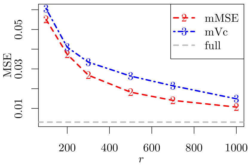
(a) 0.1493% of $y_{i}$’s are 1

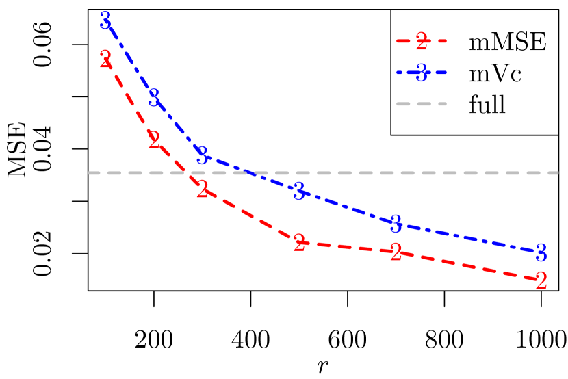
(b) 0.0111% of $y_{i}$’s are 1

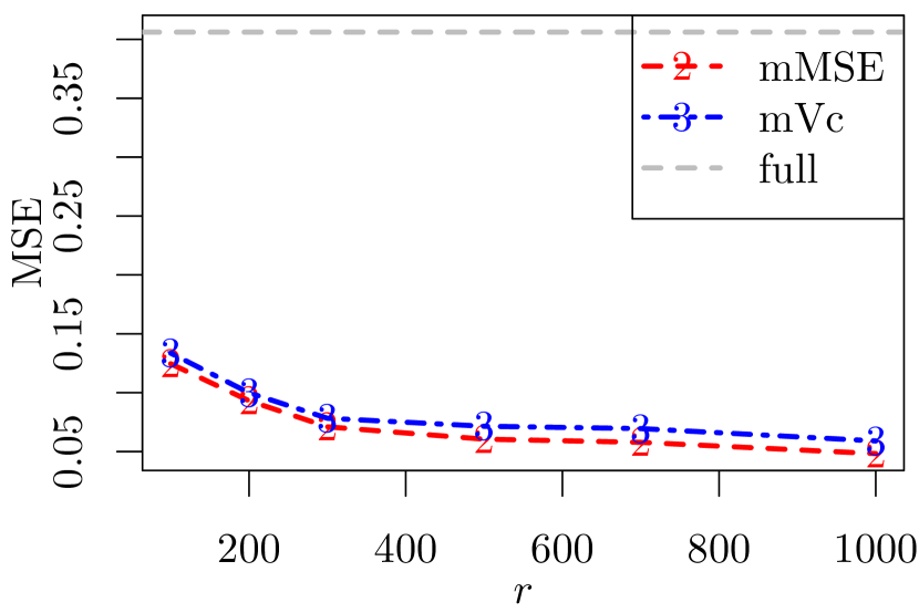
(c) 0.0008% of $y_{i}$’s are 1

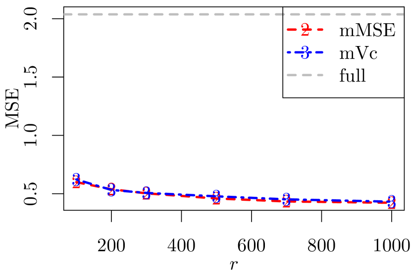
(d) 0.0002% of $y_{i}$’s are 1

Figure S.1: MSEs for rare events data with different second step subsample size $r$ and a fixed first step subsample size $r_{0}=200$, where the covariate follows the standard normal distribution.

S.2.2 Numerical results on unconditional MSEs

To calculate unconditional MSEs, we generate the full data in each repetition and then apply the subsampling methods. This way, the resultant MSEs are the unconditional MSEs. The exactly same configurations in Section 5 are used. Results are presented in Figure S.2. It is seen that the unconditional results are very similar to the conditional results, even for the imbalanced case of nzNormal data sets. For extreme imbalanced data or rare events data, the conditional MSE and the unconditional MSE can be different, as seen in the results in Section S.2.1.

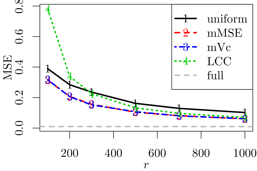
(a) mzNormal

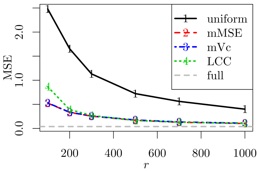
(b) nzNormal

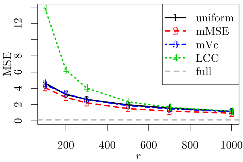
(c) ueNormal

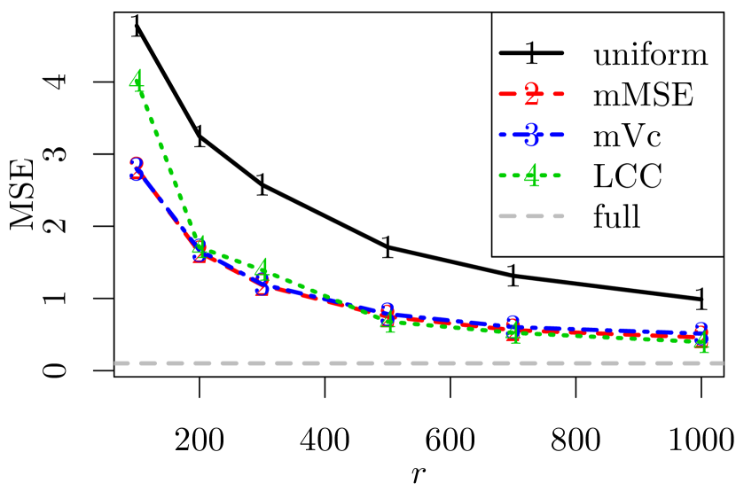
(d) mixNormal

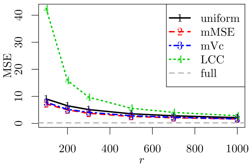
(e) $T_{3}$

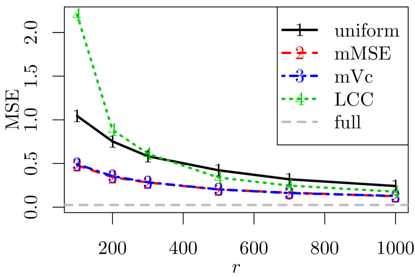
(f) EXP

Figure S.2: Unconditional MSEs for different second step subsample size ${r}$ with the first step subsample size being fixed at $r_{0}=200$.

References

- (1)
- Atkinson et al. (2007) Atkinson, A., Donev, A. and Tobias, R. (2007), Optimum experimental designs, with SAS, Vol. 34, Oxford University Press.
- Baldi et al. (2014) Baldi, P., Sadowski, P. and Whiteson, D. (2014), ‘Searching for exotic particles in high-energy physics with deep learning’, Nature Communications 5(4308), http://dx.doi.org/10.1038/ncomms5308.
- Buldygin and Kozachenko (1980) Buldygin, V. and Kozachenko, Y. V. (1980), ‘Sub-gaussian random variables’, Ukrainian Mathematical Journal 32(6), 483–489.
- Clarkson and Woodruff (2013) Clarkson, K. L. and Woodruff, D. P. (2013), Low rank approximation and regression in input sparsity time, in ‘Proceedings of the forty-fifth annual ACM symposium on Theory of computing’, ACM, pp. 81–90.
- Dhillon et al. (2013) Dhillon, P., Lu, Y., Foster, D. P. and Ungar, L. (2013), New subsampling algorithms for fast least squares regression, in ‘Advances in Neural Information Processing Systems’, pp. 360–368.
- Dines (1926) Dines, L. L. (1926), ‘Note on certain associated systems of linear equalities and inequalities’, Annals of Mathematics 28(1/4), 41–42.
- Drineas et al. (2012) Drineas, P., Magdon-Ismail, M., Mahoney, M. and Woodruff, D. (2012), ‘Faster approximation of matrix coherence and statistical leverage.’, Journal of Machine Learning Research 13, 3475–3506.
- Drineas et al. (2011) Drineas, P., Mahoney, M., Muthukrishnan, S. and Sarlos, T. (2011), ‘Faster least squares approximation.’, Numerische Mathematik 117, 219–249.
- Drineas et al. (2006) Drineas, P., Mahoney, M. W. and Muthukrishnan, S. (2006), Sampling algorithms for regression and applications, in ‘Proceedings of the seventeenth annual ACM-SIAM symposium on Discrete algorithm’, Society for Industrial and Applied Mathematics, pp. 1127–1136.
- Efron (1979) Efron, B. (1979), ‘Bootstrap methods: another look at the jackknife.’, The Annals of Statistics 7, 1–26.
- Efron and Tibshirani (1994) Efron, B. and Tibshirani, R. J. (1994), An introduction to the bootstrap, CRC press.
- Fithian and Hastie (2014) Fithian, W. and Hastie, T. (2014), ‘Local case-control sampling: Efficient subsampling in imbalanced data sets’, Annals of statistics 42(5), 1693.
- Gelman et al. (2014) Gelman, A., Carlin, J. B., Stern, H. S., Dunson, D. B., Vehtari, A. and Rubin, D. B. (2014), Bayesian data analysis, 3 edn, Chapman and Hall/CRC.
- Hosmer Jr et al. (2013) Hosmer Jr, D. W., Lemeshow, S. and Sturdivant, R. X. (2013), Applied logistic regression, Vol. 398, John Wiley & Sons.
- Kiefer (1959) Kiefer, J. (1959), ‘Optimum experimental designs’, Journal of the Royal Statistical Society. Series B 21(2), 272–319.
- King and Zeng (2001) King, G. and Zeng, L. (2001), ‘Logistic regression in rare events data’, Political analysis 9(2), 137–163.
- Kohavi (1996) Kohavi, R. (1996), Scaling up the accuracy of naive-bayes classifiers: a decision-tree hybrid, in ‘Proceedings of the Second International Conference on Knowledge Discovery and Data Mining’, pp. 202–207.
-
Lichman (2013)
Lichman, M. (2013), ‘UCI Machine Learning
Repository [http://archive.ics.uci.edu/ml]. Irvine, CA: University of
California, School of Information and Computer Science’.
http://archive.ics.uci.edu/ml - Ma et al. (2014) Ma, P., Mahoney, M. and Yu, B. (2014), A statistical perspective on algorithmic leveraging, in ‘Proceedings of the 31st International Conference on Machine Learning (ICML-14)’, pp. 91–99.
- Ma et al. (2015) Ma, P., Mahoney, M. and Yu, B. (2015), ‘A statistical perspective on algorithmic leveraging’, Journal of Machine Learning Research 16, 861–911.
- Ma and Sun (2015) Ma, P. and Sun, X. (2015), ‘Leveraging for big data regression’, Wiley Interdisciplinary Reviews: Computational Statistics 7(1), 70–76.
- Mahoney and Drineas (2009) Mahoney, M. W. and Drineas, P. (2009), ‘CUR matrix decompositions for improved data analysis’, Proceedings of the National Academy of Sciences 106(3), 697–702.
- McWilliams et al. (2014) McWilliams, B., Krummenacher, G., Lucic, M. and Buhmann, J. M. (2014), Fast and robust least squares estimation in corrupted linear models, in ‘Advances in Neural Information Processing Systems’, pp. 415–423.
- Owen (2007) Owen, A. B. (2007), ‘Infinitely imbalanced logistic regression’, The Journal of Machine Learning Research 8, 761–773.
-
R Core Team (2015)
R Core Team (2015), R: A Language and
Environment for Statistical Computing, R Foundation for Statistical
Computing, Vienna, Austria.
https://www.R-project.org/ - Rokhlin and Tygert (2008) Rokhlin, V. and Tygert, M. (2008), ‘A fast randomized algorithm for overdetermined linear least-squares regression’, Proceedings of the National Academy of Sciences 105(36), 13212–13217.
- Scott and Wild (1986) Scott, A. J. and Wild, C. J. (1986), ‘Fitting logistic models under case-control or choice based sampling’, Journal of the Royal Statistical Society. Series B 48(2), 170–182.
- Silvapulle (1981) Silvapulle, M. (1981), ‘On the existence of maximum likelihood estimators for the binomial response models’, Journal of the Royal Statistical Society. Series B 43(3), 310–313.

References

- (1)
- Ferguson (1996) Ferguson, T. S. (1996), A Course in Large Sample Theory, Chapman and Hall.
- van der Vaart (1998) van der Vaart, A. (1998), Asymptotic Statistics, Cambridge University Press, London.