A Fast Numerical Scheme for the Godunov-Peshkov-Romenski Model of Continuum Mechanics

Abstract

A new second-order numerical scheme based on an operator splitting is proposed for the Godunov-Peshkov-Romenski model of continuum mechanics. The homogeneous part of the system is solved with a finite volume method based on a WENO reconstruction, and the temporal ODEs are solved using some analytic results presented here. Whilst it is not possible to attain arbitrary-order accuracy with this scheme (as with ADER-WENO schemes used previously), the attainable order of accuracy is often sufficient, and solutions are computationally cheap when compared with other available schemes. The new scheme is compared with an ADER-WENO scheme for various test cases, and a convergence study is undertaken to demonstrate its order of accuracy.

 

1 Background

1.1 Motivation

The Godunov-Peshkov-Romenski model of continuum mechanics (as described in 1.2) presents an exciting possibility of being able to describe both fluids and solids within the same mathematical framework. This has the potential to streamline development of simulation software by reducing the number of different systems of equations that require solvers, and cutting down on the amount of theoretical work required, for example in the treatment of interfaces in multimaterial problems. In addition to this, the hyperbolic nature of the GPR model ensures that the nonphysical instantaneous transmission of information appearing in certain non-hyperbolic models (such as the Navier-Stokes equations) cannot occur. Parallelization also tends to be easier with hyperbolic models, allowing us to leverage the great advances that have been made in parallel computing architectures in recent years.

At the time of writing, the GPR model has been solved for a variety of fluid and solid problems using the ADER-WENO method (Dumbser et al. [8], Boscheri et al. [4]). ADER-WENO methods (described in 1.3) are extremely effective in producing arbitrarily-high order solutions to hyperbolic systems of PDEs, but in some situations their accompanying computational cost may prove burdensome. A new method is presented in this study that is simple to implement and computationally cheaper than a corresponding ADER-WENO method if only second order accuracy is required. This may prove useful in the design of simulation software addressing problems in which not just accuracy but also speed and usability are of paramount importance.

1.2 The GPR Model

The GPR model, first introduced in Peshkov and Romenski [23], has its roots in Godunov and Romenski’s 1970s model of elastoplastic deformation (see Godunov and Romenski [14]). It was expanded upon in Dumbser et al. [8] to include thermal conduction. This expanded model takes the following form:

$$\frac{\partial\rho}{\partial t}+\frac{\partial\left(\rho v_{k}\right)}{\partial x_{k}} =0$$ (1a)

$$\frac{\partial\left(\rho v_{i}\right)}{\partial t}+\frac{\partial(\rho v_{i}v_{k}+p\delta_{ik}-\sigma_{ik})}{\partial x_{k}} =0$$ (1b)

$$\frac{\partial A_{ij}}{\partial t}+\frac{\partial\left(A_{ik}v_{k}\right)}{\partial x_{j}}+v_{k}\left(\frac{\partial A_{ij}}{\partial x_{k}}-\frac{\partial A_{ik}}{\partial x_{j}}\right) =-\frac{\psi_{ij}}{\theta_{1}(\tau_{1})}$$ (1c)

$$\frac{\partial\left(\rho J_{i}\right)}{\partial t}+\frac{\partial\left(\rho J_{i}v_{k}+T\delta_{ik}\right)}{\partial x_{k}} =-\frac{\rho H_{i}}{\theta_{2}\left(\tau_{2}\right)}$$ (1d)

$$\frac{\partial\left(\rho E\right)}{\partial t}+\frac{\partial\left(\rho Ev_{k}+\left(p\delta_{ik}-\sigma_{ik}\right)v_{i}+q_{k}\right)}{\partial x_{k}} =0$$ (1e)

$\rho$,$\mathbf{v}$,$p$,$\delta$,$\sigma$,$T$,$E$,$\boldsymbol{q}$ retain their usual meanings. $\theta_{1}$ and $\theta_{2}$ are positive scalar functions, chosen according to the properties of the material being modeled. $A$ is the distortion tensor (containing information about the deformation and rotation of material elements), $\mathbf{J}$ is the thermal impulse vector (a thermal analogue of momentum), $\tau_{1}$ is the strain dissipation time, and $\tau_{2}$ is the thermal impulse relaxation time. $\psi=\frac{\partial E}{\partial A}$ and $\boldsymbol{H}=\frac{\partial E}{\partial\boldsymbol{J}}$.

The following definitions are given:

$$p =\rho^{2}\frac{\partial E}{\partial\rho}$$ (2a)

$$\sigma =-\rho A^{T}\frac{\partial E}{\partial A}$$ (2b)

$$T =\frac{\partial E}{\partial s}$$ (2c)

$$\boldsymbol{q} =\frac{\partial E}{\partial s}\frac{\partial E}{\partial\boldsymbol{J}}$$ (2d)

To close the system, the equation of state (EOS) must be specified, from which the above quantities and the sources can be derived. $E$ is the sum of the contributions of the energies at the molecular scale (microscale), the material element scale (mesoscale), and the flow scale (macroscale):

$$E=E_{1}\left(\rho,p\right)+E_{2}\left(A,\boldsymbol{J}\right)+E_{3}\left(\boldsymbol{v}\right)$$ (3)

The EOS used in this study (and described in the following passages) is taken from Dumbser et al. [8]. It should be noted, however, that this is just one particular choice, and there are many others that may be used.

For an ideal or stiffened gas, $E_{1}$ is given by:

$$E_{1}=\frac{p+\gamma p_{\infty}}{\left(\gamma-1\right)\rho}$$ (4)

where $p_{\infty}=0$ for an ideal gas.

$E_{2}$ is chosen to have the following quadratic form:

$$E_{2}=\frac{c_{s}^{2}}{4}\left\|\operatorname{dev}\left(G\right)\right\|_{F}^{2}+\frac{\alpha^{2}}{2}\left\|\boldsymbol{J}\right\|^{2}$$ (5)

$c_{s}$ is the characteristic velocity of propagation of transverse perturbations. $\alpha$ is a constant related to the characteristic velocity of propagation of heat waves:

$$c_{h}=\frac{\alpha}{\rho}\sqrt{\frac{T}{c_{v}}}$$ (6)

$G=A^{T}A$ is the Gramian matrix of the distortion tensor, and $\operatorname{dev}\left(G\right)$ is the deviator (trace-free part) of $G$:

$$\operatorname{dev}\left(G\right)=G-\frac{1}{3}\operatorname{tr}\left(G\right)I$$ (7)

$E_{3}$ is the usual specific kinetic energy per unit mass:

$$E_{3}=\frac{1}{2}\left\|\boldsymbol{v}\right\|^{2}$$ (8)

The following forms are chosen:

$$\theta_{1}\left(\tau_{1}\right) =\frac{\tau_{1}c_{s}^{2}}{3\left|A\right|^{\frac{5}{3}}}$$ (9a)

$$\theta_{2}\left(\tau_{2}\right) =\tau_{2}\alpha^{2}\frac{\rho T_{0}}{\rho_{0}T}$$ (9b)

$$\tau_{1} =\frac{6\mu}{\rho_{0}c_{s}^{2}}$$ (10a)

$$\tau_{2} =\frac{\rho_{0}\kappa}{T_{0}\alpha^{2}}$$ (10b)

The justification of these choices is that classical Navier–Stokes–Fourier theory is recovered in the stiff limit $\tau_{1},\tau_{2}\rightarrow 0$ (see Dumbser et al. [8]). This results in the following relations:

$$\sigma =-\rho c_{s}^{2}G\operatorname{dev}\left(G\right)$$ (11a)

$$\boldsymbol{q} =\alpha^{2}T\boldsymbol{J}$$ (11b)

$$-\frac{\psi}{\theta_{1}(\tau_{1})} =-\frac{3}{\tau_{1}}\left|A\right|^{\frac{5}{3}}A\operatorname{dev}\left(G\right)$$ (11c)

$$-\frac{\rho\boldsymbol{H}}{\theta_{2}\left(\tau_{2}\right)} =-\frac{T\rho_{0}}{T_{0}\tau_{2}}\boldsymbol{J}$$ (11d)

The following constraint also holds (see Peshkov and Romenski [23]):

$$\det\left(A\right)=\frac{\rho}{\rho_{0}}$$ (12)

The GPR model and Godunov and Romenski’s 1970s model of elastoplastic deformation in fact relie upon the same equations. The realization of Peshkov and Romenski was that these are the equations of motion for an arbitrary continuum - not just a solid - and so the model can be applied to fluids too. Unlike in previous continuum models, material elements have not only finite size, but also internal structure, encoded in the distortion tensor.

The strain dissipation time $\tau_{1}$ of the HPR model is a continuous analogue of Frenkel’s “particle settled life time” Frenkel [12]; the characteristic time taken for a particle to move by a distance of the same order of magnitude as the particle’s size. Thus, $\tau_{1}$ characterizes the time taken for a material element to rearrange with its neighbors. $\tau_{1}=\infty$ for solids and $\tau_{1}=0$ for inviscid fluids. It is in this way that the HPR model seeks to describe all three major phases of matter, as long as a continuum description is appropriate for the material at hand.

The evolution equation for $\boldsymbol{J}$ and its contribution to the energy of the system are derived from Romenski’s model of hyperbolic heat transfer, originally proposed in Malyshev and Romenskii [19], Romenski [26], and implemented in Romenski et al. [25, 24]. In this model, $\boldsymbol{J}$ is effectively defined as the variable conjugate to the entropy flux, in the sense that the latter is the derivative of the specific internal energy with respect to $\boldsymbol{J}$. Romenski remarks that it is more convenient to evolve $\boldsymbol{J}$ and $E$ than the heat flux or the entropy flux, and thus the equations take the form given here. $\tau_{2}$ characterizes the speed of relaxation of the thermal impulse due to heat exchange between material elements.

1.3 The ADER-WENO Method

The ADER-WENO method was used in Dumbser et al. [8], Boscheri et al. [4] to solve the GPR system. It produces arbitrarily high-order solutions to hyperbolic systems of PDEs and has been shown to be particularly effective for a wide range of systems (e.g. the classical Euler equations of gas dynamics, the special relativistic hydrodynamics and ideal magnetohydrodynamics equations, and the Baer-Nunziato model for compressible two-phase flow - see Balsara et al. [1], Zanotti and Dumbser [28]). The first step in the process - the WENO method - will be used later in this study and is therefore discussed in detail here. The remaining steps are described qualitatively, with references for further information given.

WENO (Weighted Essentially Non-Oscillatory) methods are used to produce high order polynomial approximations to piece-wise constant data. Many variations exist. In this study, the method of Dumbser et al. [11] is used.

Consider the domain $\left[0,L\right]$. Take $K,N\in\mathbb{N}$. The order of accuracy of the resulting method will be $N+1$. Take the set of grid points $x_{i}=\frac{i\cdot L}{K}$ for $i=0,\ldots,K$ and let $\Delta x=\frac{L}{K}$. Denote cell $\left[x_{i},x_{i+1}\right]$ by $C_{i}$. Given cell-wise constant data $u$ on $\left[0,L\right]$, an order $N$ polynomial reconstruction of $u$ in $C_{i}$ will be performed. Define the scaled space variable:

$$\chi^{i}=\frac{1}{\Delta x}\left(x-x_{i}\right)$$ (13)

Denoting the Gauss-Legendre abscissae on $\left[0,1\right]$ by $\left\{\chi_{0},\ldots,\chi_{N}\right\}$, define the nodal basis of order $N$: the Lagrange interpolating polynomials $\left\{\psi_{0},\ldots,\psi_{N}\right\}$ with the following property:

$$\psi_{i}\left(\chi_{j}\right)=\delta_{ij}$$ (14)

If $N$ is even, take the stencils:

$$\begin{cases}S_{1}&=\left\{C_{i-\frac{N}{2}},\ldots,C_{i+\frac{N}{2}}\right\}\\ S_{2}&=\left\{C_{i-N},\ldots,C_{i}\right\}\\ S_{3}&=\left\{C_{i},\ldots,C_{i+N}\right\}\end{cases}$$ (15)

If $N$ is odd, take the stencils:

$$\begin{cases}S_{1}&=\left\{C_{i-\left\lfloor\frac{N}{2}\right\rfloor},\ldots,C_{i+\left\lceil\frac{N}{2}\right\rceil}\right\}\\ S_{2}&=\left\{C_{i-\left\lceil\frac{N}{2}\right\rceil},\ldots,C_{i+\left\lfloor\frac{N}{2}\right\rfloor}\right\}\\ S_{3}&=\left\{C_{i-N},\ldots,C_{i}\right\}\\ S_{4}&=\left\{C_{i},\ldots,C_{i+N}\right\}\end{cases}$$ (16)

The data is reconstructed on $S_{j}$ as:

$$\sum_{p}\psi_{p}\left(\chi^{i}\left(x\right)\right)\hat{w}_{p}^{ij}$$ (17)

where the $\hat{w}_{p}^{ij}$ are solutions to the following linear system:

$$\frac{1}{\Delta x}\int_{x_{k}}^{x_{k+1}}\sum_{p}\psi_{p}\left(\chi^{k}\left(x\right)\right)\hat{w}_{p}^{ij}dx=u_{k}\qquad\forall C_{k}\in S_{j}$$ (18)

where $u_{k}$ is the value of $u$ in $C_{k}$. This can be written as $M_{j}\boldsymbol{\hat{w}^{ij}}=\boldsymbol{u_{\left[j_{0}:j_{N}\right]}}$ where $\left\{j_{0},\ldots,j_{N}\right\}$ indexes the cells in $S_{j}$. In this study reconstructions with $N=2$ are used. The matrices of these linear systems are given in 8.3, along with their inverses, which are precomputed to accelerate the solution of these systems.

Define the oscillation indicator matrix:

$$\Sigma_{mn}=\sum_{\alpha=1}^{N}\int_{0}^{1}\psi_{m}^{\left(\alpha\right)}\psi_{n}^{\left(\alpha\right)}d\chi$$ (19)

and the oscillation indicator for each stencil:

$$o_{j}=\Sigma_{mn}\hat{w}_{m}^{ij}\hat{w}_{n}^{ij}$$ (20)

The full reconstruction in $C_{i}$ is:

$$w_{i}\left(x\right)=\sum_{p}\psi_{p}\left(\chi^{i}\left(x\right)\right)\bar{w}_{p}^{i}$$ (21)

where $\bar{w}_{p}^{i}=\omega_{j}\hat{w}_{p}^{ij}$ is the weighted coefficient of the $p$th basis function, with weights:

$$\omega_{j}=\frac{\tilde{\omega}_{j}}{\sum_{k}\tilde{\omega}_{k}}\qquad\tilde{\omega}_{j}=\frac{\zeta_{j}}{\left(o_{j}+\varepsilon\right)^{r}}$$ (22)

In this study, $r=8$, $\varepsilon=10^{-14}$, $\zeta_{j}=10^{5}$ if $S_{j}$ is a central stencil, and $\zeta_{j}=1$ if $S_{j}$ is a side stencil, as in Dumbser et al. [7].

The reconstruction can be extended to two dimensions by taking:

$$\upsilon^{i}=\frac{1}{\Delta y}\left(y-y_{i}\right)$$ (23)

and defining stencils in the y-axis in an analogous manner. The data in $C_{i}$ is then reconstructed using stencil $S_{j}$ as:

$$\sum_{p,q}\psi_{p}\left(\chi^{i}\left(x\right)\right)\psi_{q}\left(\upsilon^{i}\left(x\right)\right)\tilde{w}_{pq}^{ij}$$ (24)

where the coefficients of the weighted 1D reconstruction are used as cell averages:

$$M_{j}\boldsymbol{\tilde{w}_{p}^{ij}}=\boldsymbol{\bar{w}_{p}^{\left[j_{0}:j_{N}\right]}}\qquad\forall p\in\left\{0,\ldots,N\right\}$$ (25)

The oscillation indicator is calculated for each $p$ in the same manner as the 1D case. The reconstruction method is easily further extensible to three dimensions, now using the coefficients $\bar{w}_{pq}$ of the weighted 2D reconstruction as cell averages.

The next process in the ADER-WENO method is to perform a Continuous Galerkin or Discontinuous Galerkin spatio-temporal polynomial reconstruction of the data in each cell, using the WENO reconstruction as initial data at the start of the time step (see Balsara et al. [1] and Dumbser et al. [5] respectively for implementations of these two variations). The order of this reconstruction in time is usually taken to be the same as the spatial order, and the same basis polynomials are used. The process involves finding the root of a non-linear system, and this process is guaranteed to converge in exact arithmetic for certain classes of PDEs (see Jackson [16]). This root finding can be computationally expensive relative to the WENO reconstruction, especially if the source terms of the PDE system are stiff.

The final step in the ADER-WENO method is to perform a finite volume update of the data in each cell, using the boundary-extrapolated values of the cell-local Galerkin reconstructions to calculate the flux terms, and the interior values of the Galerkin reconstructions to calculate the interior volume integrals. See Dumbser et al. [7] for more details.

2 An Alternative Numerical Scheme

Note that (1a), (1b), (1c), (1d), (1e) can be written in the following form:

$$\frac{\partial\boldsymbol{Q}}{\partial t}+\boldsymbol{\nabla}\cdot\boldsymbol{F}\left(\boldsymbol{Q}\right)+\boldsymbol{B}\left(\boldsymbol{Q}\right)\cdot\nabla\boldsymbol{Q}=\boldsymbol{S}\left(\boldsymbol{Q}\right)$$ (26)

As described in Toro [27], a viable way to solve inhomogeneous systems of PDEs is to employ an operator splitting. That is, the following subsystems are solved:

$$\frac{\partial\boldsymbol{Q}}{\partial t}+\boldsymbol{\nabla}\cdot\boldsymbol{F}\left(\boldsymbol{Q}\right)+\boldsymbol{B}\left(\boldsymbol{Q}\right)\cdot\nabla\boldsymbol{Q} =\boldsymbol{0}$$ (27a)

$$\frac{d\boldsymbol{Q}}{dt} =\boldsymbol{S}\left(\boldsymbol{Q}\right)$$ (27b)

The advantage of this approach is that specialized solvers can be employed to compute the results of the different subsystems. Let $H^{\delta t},S^{\delta t}$ be the operators that take data $\boldsymbol{Q}\left(x,t\right)$ to $\boldsymbol{Q}\left(x,t+\delta t\right)$ under systems (27a) and (27b) respectively. A second-order scheme (in time) for solving the full set of PDEs over time step $\left[0,\Delta t\right]$ is obtained by calculating $\boldsymbol{Q_{\Delta t}}$ using a Strang splitting:

$$\boldsymbol{Q_{\Delta t}}=S^{\frac{\Delta t}{2}}H^{\Delta t}S^{\frac{\Delta t}{2}}\boldsymbol{Q_{0}}$$ (28)

In the scheme proposed here, the homogeneous subsystem will be solved using a WENO reconstruction of the data, followed by a finite volume update, and the temporal ODEs will be solved with appropriate ODE solvers. This new scheme will be referred to here as the Split-WENO method.

2.1 The Homogeneous System

A WENO reconstruction of the cell-averaged data is performed at the start of the time step (as described in 1.3). Focusing on a single cell $C_{i}$ at time $t_{n}$, we have $\boldsymbol{w^{n}}\left(\boldsymbol{x}\right)=\boldsymbol{w^{n}}_{p}\Psi_{p}\left(\boldsymbol{\chi}\left(\boldsymbol{x}\right)\right)$ in $C_{i}$ where $\Psi_{p}$ is a tensor product of basis functions in each of the spatial dimensions. The flux in $C$ is approximated by $\boldsymbol{F}\left(\boldsymbol{x}\right)\approx\boldsymbol{F}\left(\boldsymbol{w}_{p}\right)\Psi_{p}\left(\boldsymbol{\chi}\left(\boldsymbol{x}\right)\right)$. $\boldsymbol{w}_{p}$ are stepped forwards half a time step using the update formula:

$$\frac{\boldsymbol{w_{p}^{n+\frac{1}{2}}}-\boldsymbol{w_{p}^{n}}}{\Delta t/2}+\boldsymbol{F}\left(\boldsymbol{w_{k}^{n}}\right)\cdot\nabla\Psi_{k}\left(\boldsymbol{\chi_{p}}\right)+\boldsymbol{B}\left(\boldsymbol{w_{p}^{n}}\right)\cdot\left(\boldsymbol{w_{k}^{n}}\nabla\Psi_{k}\left(\boldsymbol{\chi_{p}}\right)\right)=\boldsymbol{0}$$ (29)

i.e.

$$\boldsymbol{w_{p}^{n+\frac{1}{2}}}=\boldsymbol{w_{p}^{n}}-\frac{\Delta t}{2\Delta x}\left(\boldsymbol{F}\left(\boldsymbol{w_{k}^{n}}\right)\cdot\nabla\Psi_{k}\left(\boldsymbol{\chi_{p}}\right)+\boldsymbol{B}\left(\boldsymbol{w_{p}^{n}}\right)\cdot\left(\boldsymbol{w_{k}^{n}}\nabla\Psi_{k}\left(\boldsymbol{\chi_{p}}\right)\right)\right)$$ (30)

where $\boldsymbol{\chi_{p}}$ is the node corresponding to $\Psi_{p}$. This evolution to the middle of the time step is similar to that used in the second-order MUSCL and SLIC schemes (see Toro [27]) and, as with those schemes, it is integral to giving the method presented here its second-order accuracy.

Integrating (27a) over $C$ gives:

$$\boldsymbol{Q_{i}^{n+1}}=\boldsymbol{Q_{i}^{n}}-\Delta t_{n}\left(\boldsymbol{P_{i}^{n+\frac{1}{2}}}+\boldsymbol{D_{i}^{n+\frac{1}{2}}}\right)$$ (31)

where

$$\boldsymbol{Q_{i}^{n}} =\frac{1}{V}\int_{C}\boldsymbol{Q}\left(\boldsymbol{x},t_{n}\right)d\boldsymbol{x}$$ (32a)

$$\boldsymbol{P_{i}^{n+\frac{1}{2}}} =\frac{1}{V}\int_{C}\boldsymbol{B}\left(\boldsymbol{Q}\left(\boldsymbol{x},t_{n+\frac{1}{2}}\right)\right)\cdot\nabla\boldsymbol{Q}\left(\boldsymbol{x},t_{n+\frac{1}{2}}\right)d\boldsymbol{x}$$ (32b)

$$\boldsymbol{D_{i}^{n+\frac{1}{2}}} =\frac{1}{V}\oint_{\partial C}\boldsymbol{\mathcal{D}}\left(\boldsymbol{Q^{-}}\left(\boldsymbol{s},t_{n+\frac{1}{2}}\right),\boldsymbol{Q^{+}}\left(\boldsymbol{s},t_{n+\frac{1}{2}}\right)\right)d\boldsymbol{s}$$ (32c)

where $V$ is the volume of $C$ and $\boldsymbol{Q^{-},Q^{+}}$ are the interior and exterior extrapolated states at the boundary of $C$, respectively.

Note that (27a) can be rewritten as:

$$\frac{\partial\boldsymbol{Q}}{\partial t}+\boldsymbol{M}\left(\boldsymbol{Q}\right)\cdot\nabla\boldsymbol{Q}=\boldsymbol{0}$$ (33)

where $\boldsymbol{M}=\frac{\partial\boldsymbol{F}}{\partial\boldsymbol{Q}}+\boldsymbol{B}$. Let $\boldsymbol{n}$ be the normal to the boundary at point $\boldsymbol{s}\in\partial C$. For the GPR model, $\hat{M}=\boldsymbol{M}\left(\boldsymbol{Q}\left(\boldsymbol{s}\right)\right)\cdot\boldsymbol{n}$ is a diagonalizable matrix with decomposition $\hat{M}=\hat{R}\hat{\Lambda}\hat{R}^{-1}$ where the columns of $\hat{R}$ are the right eigenvectors and $\hat{\Lambda}$ is the diagonal matrix of eigenvalues. Define also $\boldsymbol{\hat{F}}=\boldsymbol{F}\cdot\boldsymbol{n}$ and $\hat{B}=\boldsymbol{B}\cdot\boldsymbol{n}$. Using these definitions, the interface terms arising in the FV formula have the following form:

$$\boldsymbol{\mathcal{D}}\left(\boldsymbol{Q^{-}},\boldsymbol{Q^{+}}\right)=\frac{1}{2}\left(\boldsymbol{\hat{F}}\left(\boldsymbol{Q^{+}}\right)+\boldsymbol{\hat{F}}\left(\boldsymbol{Q^{-}}\right)+\tilde{B}\left(\boldsymbol{Q^{+}}-\boldsymbol{Q^{-}}\right)+\tilde{M}\left(\boldsymbol{Q^{+}}-\boldsymbol{Q^{-}}\right)\right)$$ (34)

$\tilde{M}$ is chosen to either correspond to a Rusanov/Lax-Friedrichs flux (see Toro [27]):

$$\tilde{M}=\max\left(\max\left|\hat{\Lambda}\left(\boldsymbol{Q^{+}}\right)\right|,\max\left|\hat{\Lambda}\left(\boldsymbol{Q^{-}}\right)\right|\right)$$ (35)

or a simplified Osher–Solomon flux (see Dumbser and Toro [9, 10]):

$$\tilde{M}=\int_{0}^{1}\left|\hat{M}\left(\boldsymbol{Q^{-}}+z\left(\boldsymbol{Q^{+}}-\boldsymbol{Q^{-}}\right)\right)\right|dz$$ (36)

where

$$\left|\hat{M}\right|=\hat{R}\left|\hat{\Lambda}\right|\hat{R}^{-1}$$ (37)

$\tilde{B}$ takes the following form:

$$\tilde{B}=\int_{0}^{1}\hat{B}\left(\boldsymbol{Q^{-}}+z\left(\boldsymbol{Q^{+}}-\boldsymbol{Q^{-}}\right)\right)dz$$ (38)

It was found that the Osher-Solomon flux would often produce slightly less diffusive results, but that it was more computationally expensive, and also had a greater tendency to introduce numerical artefacts.

$\boldsymbol{P_{i}^{n+\frac{1}{2}}},\boldsymbol{D_{i}^{n+\frac{1}{2}}}$ are calculated using an $N+1$-point Gauss-Legendre quadrature, replacing $\boldsymbol{Q}\left(\boldsymbol{x},t_{n+\frac{1}{2}}\right)$ with $\boldsymbol{w^{n+\frac{1}{2}}}\left(\boldsymbol{x}\right)$.

2.2 The Temporal ODEs

Noting that $\frac{d\rho}{dt}=0$ over the ODE time step, the operator $S$ entails solving the following systems:

$$\frac{dA}{dt} =\frac{-3}{\tau_{1}}\left|A\right|^{\frac{5}{3}}A\operatorname{dev}\left(G\right)$$ (39a)

$$\frac{d\boldsymbol{J}}{dt} =-\frac{1}{\tau_{2}}\frac{T\rho_{0}}{T_{0}\rho}\boldsymbol{J}$$ (39b)

These systems can be solved concurrently with a stiff ODE solver. The Jacobians of these two systems to be used in an ODE solver are given in 8.1 and 8.2. However, these systems can also be solved separately, using the analytical results presented in Section 3, under specific assumptions. The second-order Strang splitting is then:

$$\boldsymbol{Q_{\Delta t}}=D^{\frac{\Delta t}{2}}T^{\frac{\Delta t}{2}}H^{\Delta t}T^{\frac{\Delta t}{2}}D^{\frac{\Delta t}{2}}\boldsymbol{Q_{0}}$$ (40)

where $D^{\delta t},T^{\delta t}$ are the operators solving the distortion and thermal impulse ODEs respectively, over timestep $\delta t$. This allows us to bypass the relatively computationally costly process of solving these systems numerically.

3 GPR-Specific Performance Improvements

3.1 The Thermal Impulse ODEs

Taking the EOS for the GPR model (3) and denoting by $E_{2}^{\left(A\right)},E_{2}^{\left(J\right)}$ the components of $E_{2}$ depending on $A$ and $\boldsymbol{J}$ respectively, we have:

$$T =\frac{E_{1}}{c_{v}}$$ (41)

$$=\frac{E-E_{2}^{\left(A\right)}\left(A\right)-E_{3}\left(\boldsymbol{v}\right)}{c_{v}}-\frac{1}{c_{v}}E_{2}^{\left(J\right)}\left(\boldsymbol{J}\right)$$

$$=c_{1}-c_{2}\left\|\boldsymbol{J}\right\|^{2}$$

where:

$$c_{1} =\frac{E-E_{2}^{\left(A\right)}\left(A\right)-E_{3}\left(\boldsymbol{v}\right)}{c_{v}}$$ (42a)

$$c_{2} =\frac{\alpha^{2}}{2c_{v}}$$ (42b)

Over the time period of the ODE (39b), $c_{1},c_{2}>0$ are constant. We have:

$$\frac{dJ_{i}}{dt}=-\left(\frac{1}{\tau_{2}}\frac{\rho_{0}}{T_{0}\rho}\right)J_{i}\left(c_{1}-c_{2}\left\|\boldsymbol{J}\right\|^{2}\right)$$ (43)

Therefore:

$$\frac{d}{dt}\left(J_{i}^{2}\right)=J_{i}^{2}\left(-a+b\left(J_{1}^{2}+J_{2}^{2}+J_{3}^{2}\right)\right)$$ (44)

where

$$a =\frac{2\rho_{0}}{\tau_{2}T_{0}\rho c_{v}}\left(E-E_{2}^{\left(A\right)}\left(A\right)-E_{3}\left(\boldsymbol{v}\right)\right)$$ (45a)

$$b =\frac{\rho_{0}\alpha^{2}}{\tau_{2}T_{0}\rho c_{v}}$$ (45b)

Note that this is a generalized Lotka-Volterra system in $\left\{J_{1}^{2},J_{2}^{2},J_{3}^{2}\right\}$. It has the following analytical solution:

$$\boldsymbol{J}\left(t\right)=\boldsymbol{J}\left(0\right)\sqrt{\frac{1}{e^{at}-\frac{b}{a}\left(e^{at}-1\right)\left\|\boldsymbol{J}\left(0\right)\right\|^{2}}}$$ (46)

3.2 The Distortion ODEs

3.2.1 Reduced Distortion ODEs

Let $k_{0}=\frac{3}{\tau_{1}}\left(\frac{\rho}{\rho_{0}}\right)^{\frac{5}{3}}>0$ and let $A$ have singular value decomposition $U\Sigma V^{T}$. Then:

$$G=\left(U\Sigma V^{T}\right)^{T}U\Sigma V^{T}=V\Sigma^{2}V^{T}$$ (47)

$$\operatorname{tr}\left(G\right)=\operatorname{tr}\left(V\Sigma^{2}V^{T}\right)=\operatorname{tr}\left(\Sigma^{2}V^{T}V\right)=\operatorname{tr}\left(\Sigma^{2}\right)$$ (48)

Therefore:

$$\frac{dA}{dt} =-k_{0}U\Sigma V^{T}\left(V\Sigma^{2}V^{T}-\frac{\operatorname{tr}\left(\Sigma^{2}\right)}{3}I\right)$$ (49)

$$=-k_{0}U\Sigma\left(\Sigma^{2}-\frac{\operatorname{tr}\left(\Sigma^{2}\right)}{3}\right)V^{T}$$

$$=-k_{0}U\Sigma\operatorname{dev}\left(\Sigma^{2}\right)V^{T}$$

It is a common result (see Giles [13]) that:

$$d\Sigma=U^{T}dAV$$ (50)

and thus:

$$\frac{d\Sigma}{dt}=-k_{0}\Sigma\operatorname{dev}\left(\Sigma^{2}\right)$$ (51)

Using a fast $3\times 3$ SVD algorithm (such as in McAdams et al. [20]), $U,V,\Sigma$ can be obtained, after which the following procedure is applied to $\Sigma$, giving $A\left(t\right)=U\Sigma\left(t\right)V^{T}$.

Denote the singular values of $A$ by $a_{1},a_{2},a_{3}$. Then:

$$\Sigma\operatorname{dev}\left(\Sigma^{2}\right)=\left(\begin{array}[]{ccc}a_{1}\left(a_{1}^{2}-\frac{a_{1}^{2}+a_{2}^{2}+a_{3}^{2}}{3}\right)&0&0\\ 0&a_{1}\left(a_{1}^{2}-\frac{a_{1}^{2}+a_{2}^{2}+a_{3}^{2}}{3}\right)&0\\ 0&0&a_{1}\left(a_{1}^{2}-\frac{a_{1}^{2}+a_{2}^{2}+a_{3}^{2}}{3}\right)\end{array}\right)$$ (52)

Letting $x_{i}=\frac{a_{i}^{2}}{\det\left(A\right)^{\frac{2}{3}}}=\frac{a_{i}^{2}}{\left(\frac{\rho}{\rho_{0}}\right)^{\frac{2}{3}}}$ we have:

$$\frac{dx_{i}}{d\tau}=-3x_{i}\left(x_{i}-\bar{x}\right)$$ (53)

where $\tau=\frac{2}{\tau_{1}}\left(\frac{\rho}{\rho_{0}}\right)^{\frac{7}{3}}t$ and $\bar{x}$ is the arithmetic mean of $x_{1},x_{2},x_{3}$. This ODE system travels along the surface $\Psi=\left\{x_{1},x_{2},x_{3}>0,x_{1}x_{2}x_{3}=1\right\}$ to the point $x_{1},x_{2},x_{3}=1$. This surface is symmetrical in the planes $x_{1}=x_{2}$, $x_{1}=x_{3}$, $x_{2}=x_{3}$. As such, given that the system is autonomous, the paths of evolution of the $x_{i}$ cannot cross the intersections of these planes with $\Psi$. Thus, any non-strict inequality of the form $x_{i}\geq x_{j}\geq x_{k}$ is maintained for the whole history of the system. By considering (53) it is clear that in this case $x_{i}$ is monotone decreasing, $x_{k}$ is monotone increasing, and the time derivative of $x_{j}$ may switch sign.

Note that we have:

$$\left\{\begin{array}[]{c}\frac{dx_{i}}{d\tau}=-x_{i}\left(2x_{i}-x_{j}-x_{k}\right)=-x_{i}\left(2x_{i}-x_{j}-\frac{1}{x_{i}x_{j}}\right)\\ \frac{dx_{j}}{d\tau}=-x_{j}\left(2x_{j}-x_{k}-x_{i}\right)=-x_{j}\left(2x_{j}-x_{i}-\frac{1}{x_{i}x_{j}}\right)\end{array}\right.$$ (54)

Thus, an ODE solver can be used on these two equations to effectively solve the ODEs for all 9 components of $A$. Note that:

$$\frac{dx_{j}}{dx_{i}}=\frac{x_{j}}{x_{i}}\frac{2x_{j}-x_{i}-\frac{1}{x_{i}x_{j}}}{2x_{i}-x_{j}-\frac{1}{x_{i}x_{j}}}$$ (55)

This has solution:

$$x_{j}=\frac{c+\sqrt{c^{2}+4\left(1-c\right)x_{i}^{3}}}{2x_{i}^{2}}$$ (56)

where

$$c=-\frac{x_{i,0}\left(x_{i,0}x_{j,0}^{2}-1\right)}{x_{i,0}-x_{j,0}}\in\left(-\infty,0\right]$$ (57)

In the case that $x_{i,0}=x_{j,0}$, we have $x_{i}=x_{j}$ for all time. Thus, the ODE system for $A$ has been reduced to a single ODE, as $x_{j}\left(x_{i}\right)$ can be inserted into the RHS of the equation for $\frac{dx_{i}}{d\tau}$. However, it is less computationally expensive to evolve the system presented in (54).

3.2.2 Bounds on Reduced Distortion ODEs

If any of the relations in $x_{i}\geq x_{j}\geq x_{k}$ are in fact equalities, equality is maintained throughout the history of the system. This can be seen by noting that the time derivatives of the equal variables are in this case equal. If $x_{j}=x_{k}$ then $x_{i}=\frac{1}{x_{j}^{2}}$. Combining these results, the path of the system in $\left(x_{i},x_{j}\right)$ coordinates is in fact confined to the curved triangular region:

$$\left\{\left(x_{i},x_{j}\right):x_{i}\leq x_{i}^{0}\>\cap\>x_{i}\geq x_{j}\>\cap\>x_{i}\geq\frac{1}{x_{j}^{2}}\right\}$$ (58)

Figure 1: The (shaded) region to which $x_{i},x_{j}$ are confined in the evolution of the distortion ODEs

This is demonstrated in Figure 1 on page 1. By (54), the rate of change of $x_{i}$ at a particular value $x_{i}=x_{i}^{*}$ is given by:

$$-x_{i}^{*}\left(2x_{i}^{*}-x_{j}-\frac{1}{x_{i}^{*}x_{j}}\right)$$ (59)

Note that:

$$\frac{d}{dx_{j}}\left(2x_{i}^{*}-x_{j}-\frac{1}{x_{i}^{*}x_{j}}\right) =-1+\frac{1}{x_{i}^{*}x_{j}^{2}}=0$$ (60)

$$\Rightarrow x_{j}=\frac{1}{\sqrt{x_{i}^{*}}}$$

$$\frac{d^{2}}{dx_{j}^{2}}\left(2x_{i}^{*}-x_{j}-\frac{1}{x_{i}^{*}x_{j}}\right)=\frac{-2}{x_{i}^{*}x_{j}^{3}}<0$$ (61)

Thus, $x_{i}$ decreases fastest on the line $x_{i}=\frac{1}{x_{j}^{2}}$ (the bottom boundary of the region given in Figure 1 on page 1), and slowest on the line $x_{i}=x_{j}$. The rates of change of $x_{i}$ along these two lines are given respectively by:

$$\frac{dx_{i}}{d\tau} =-2x_{i}\left(x_{i}-\sqrt{\frac{1}{x_{i}}}\right)$$ (62a)

$$\frac{dx_{i}}{d\tau} =-x_{i}\left(x_{i}-\frac{1}{x_{i}^{2}}\right)$$ (62b)

These have implicit solutions:

$$\tau =\left(f\left(\sqrt{x_{i}}\right)+g\left(\sqrt{x_{i}}\right)\right)-\left(f\left(\sqrt{x_{i}^{0}}\right)+g\left(\sqrt{x_{i}^{0}}\right)\right)\equiv F_{1}\left(x_{i};x_{i}^{0}\right)$$ (63a)

$$\tau =\left(f\left(x_{i}\right)-g\left(x_{i}\right)\right)-\left(f\left(x_{i}^{0}\right)-g\left(x_{i}^{0}\right)\right)\equiv F_{2}\left(x_{i};x_{i}^{0}\right)$$ (63b)

where

$$f\left(x_{i}\right) =\frac{1}{6}\log\left(\frac{x_{i}^{2}+x_{i}+1}{\left(x_{i}-1\right)^{2}}\right)$$ (64a)

$$g\left(x_{i}\right) =\frac{1}{\sqrt{3}}\tan^{-1}\left(\frac{2x_{i}+1}{\sqrt{3}}\right)$$ (64b)

As (53) is an autonomous system of ODEs, it has the property that its limit $x_{1}=x_{2}=x_{3}=1$ is never obtained in finite time, in precise arithmetic. In floating point arithmetic we may say that the system has converged when $x_{i}-1<\epsilon$ (machine epsilon) for each $i$. This happens when:

$$\tau>F_{2}\left(1+\epsilon;x_{i}^{0}\right)$$ (65)

This provides a quick method to check whether it is necessary to run the ODE solver in a particular cell. If the following condition is satisfied then we know the system in that cell converges to the ground state over the time interval in which the ODE system is calculated:

$$\frac{2}{\tau_{1}}\left(\frac{\rho}{\rho_{0}}\right)^{\frac{7}{3}}\Delta t>F_{2}\left(1+\epsilon;\max\left\{x_{i}^{0}\right\}\right)$$ (66)

If the fluid is very inviscid, resulting in a stiff ODE, the critical time is lower, and there is more chance that the ODE system in the cell reaches its limit in $\Delta t$. This check potentially saves a lot of computationally expensive stiff ODE solves. The same goes for if the flow is slow-moving, as the system will be closer to its ground state at the start of the time step and is more likely to converge over $\Delta t$. Similarly, if the following condition is satisfied then we know for sure that an ODE solver is necessary, as the system certainly will not have converged over the timestep:

$$\frac{2}{\tau_{1}}\left(\frac{\rho}{\rho_{0}}\right)^{\frac{7}{3}}\Delta t<F_{1}\left(1+\epsilon;\max\left\{x_{i}^{0}\right\}\right)$$ (67)

3.2.3 Analytical Approximation

We now explore cases when even the reduced ODE system (54) need not be solved numerically. Define the following variables:

$$m =\frac{x_{1}+x_{2}+x_{3}}{3}$$ (68a)

$$u =\frac{\left(x_{1}-x_{2}\right)^{2}+\left(x_{2}-x_{3}\right)^{2}+\left(x_{3}-x_{1}\right)^{2}}{3}$$ (68b)

It is a standard result that $m\geq\sqrt[3]{x_{1}x_{2}x_{3}}$. Thus, $m\geq 1$. Note that $u$ is proportional to the internal energy contribution from the distortion. From (53) we have:

$$\frac{du}{d\tau} =-18\left(1-m\left(m^{2}-\frac{5}{6}u\right)\right)$$ (69a)

$$\frac{dm}{d\tau} =-u$$ (69b)

Combining these equations, we have:

$$\frac{d^{2}m}{d\tau^{2}}=-\frac{du}{d\tau}=18\left(1-m\left(m^{2}-\frac{5}{6}u\right)\right)$$ (70)

Therefore:

$$\left\{\begin{array}[]{c}\frac{d^{2}m}{d\tau^{2}}+15m\frac{dm}{d\tau}+18\left(m^{3}-1\right)=0\\ m\left(0\right)=m_{0}\\ m^{{}^{\prime}}\left(0\right)=-u_{0}\end{array}\right.$$ (71)

We make the following assumption, noting that it is true in all physical situations tested in this study:

$$m\left(t\right)=1+\eta\left(t\right),\quad\eta\ll 1\;\forall t\geq 0$$ (72)

Thus, we have the linearized ODE:

$$\left\{\begin{array}[]{c}\frac{d^{2}\eta}{d\tau^{2}}+15\frac{d\eta}{d\tau}+54\eta=0\\ \eta\left(0\right)=m_{0}-1\\ \eta^{{}^{\prime}}\left(0\right)=-u_{0}\end{array}\right.$$ (73)

This is a Sturm-Liouville equation with solution:

$$\eta\left(\tau\right)=\frac{e^{-9\tau}}{3}\left(\left(9m_{0}-u_{0}-9\right)e^{3\tau}-\left(6m_{0}-u_{0}-6\right)\right)$$ (74)

Thus, we also have:

$$u\left(\tau\right)=e^{-9\tau}\left(e^{3\tau}\left(18m_{0}-2u_{0}-18\right)-\left(18m_{0}-3u_{0}-18\right)\right)$$ (75)

Once $m_{\Delta t}=1+\eta\left(\frac{2}{\tau_{1}}\left(\frac{\rho}{\rho_{0}}\right)^{\frac{7}{3}}\Delta t\right)$ and $u_{\Delta t}=u\left(\frac{2}{\tau_{1}}\left(\frac{\rho}{\rho_{0}}\right)^{\frac{7}{3}}\Delta t\right)$ have been found, we have:

$$\frac{x_{i}+x_{j}+x_{k}}{3} =m_{\Delta t}$$ (76a)

$$\frac{\left(x_{i}-x_{j}\right)^{2}+\left(x_{j}-x_{k}\right)^{2}+\left(x_{k}-x_{i}\right)^{2}}{3} =u_{\Delta t}$$ (76b)

$$x_{i}x_{j}x_{k} =1$$ (76c)

This gives:

$$x_{i} =\frac{\sqrt[3]{6\left(\sqrt{81\Delta^{2}-6u_{\Delta t}^{3}}+9\Delta\right)}}{6}+\frac{u_{\Delta t}}{\sqrt[3]{6\left(\sqrt{81\Delta^{2}-6u_{\Delta t}^{3}}+9\Delta\right)}}+m_{\Delta t}$$ (77a)

$$x_{j} =\frac{1}{2}\left(\sqrt{\frac{x_{i}\left(3m_{\Delta t}-x_{i}\right)^{2}-4}{x_{i}}}+3m_{\Delta t}-x_{i}\right)$$ (77b)

$$x_{k} =\frac{1}{x_{i}x_{j}}$$ (77c)

where

$$\Delta=-2m_{\Delta t}^{3}+m_{\Delta t}u_{\Delta t}+2$$ (78)

Note that taking the real parts of the above expression for $x_{i}$ gives:

$$x_{i} =\frac{\sqrt{6u_{\Delta t}}}{3}\cos\left(\frac{\theta}{3}\right)+m_{\Delta t}$$ (79a)

$$\theta =\tan^{-1}\left(\frac{\sqrt{6u_{\Delta t}^{3}-81\Delta^{2}}}{9\Delta}\right)$$ (79b)

At this point it is not clear which values of $\left\{x_{i},x_{j},x_{k}\right\}$ are taken by $x_{1},x_{2},x_{3}$. However, this can be inferred from the fact that any relation $x_{i}\geq x_{j}\geq x_{k}$ is maintained over the lifetime of the system. Thus, the stiff ODE solver has been obviated by a few arithmetic operations.

4 Numerical Results

4.1 Strain Relaxation

In this section, the approximate analytic solver for the distortion ODEs, presented in 3.2.3, is compared with a numerical ODE solver. Initial data was taken from Barton and Drikakis [2]:

$$A=\left(\begin{array}[]{ccc}1&0&0\\ -0.01&0.95&0.02\\ -0.015&0&0.9\end{array}\right)^{-1}$$ (80)

Additionally, the following parameter values were used: $\rho_{0}=1,c_{s}=1,\mu=10^{-2}$, giving $\tau_{1}=0.06$. As can be seen in Figure 2 on page 2, Figure 3 on page 3, and Figure 4 on page 4, the approximate analytic solver compares well with the numerical solver in its results for the distortion tensor $A$, and thus also the internal energy and stress tensor. The numerical ODE solver was the odeint solver from SciPy 0.18.1, based on the LSODA solver from the FORTRAN library ODEPACK (see Oliphant [22]).

Figure 2: The components of the distortion tensor in the Strain Relaxation Test

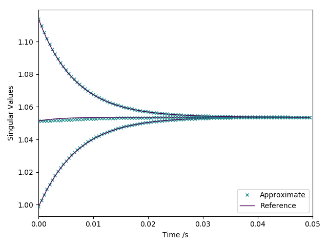
Figure 3: The singular values of the distortion tensor and the energy in the Strain Relaxation Test

Figure 4: The components of the stress tensor in the Strain Relaxation Test

4.2 Stokes’ First Problem

This problem is one of the few test cases with an analytic solution for the Navier-Stokes equations. It consists of two ideal gases in an infinite domain, meeting at the plane $x=0$, initially flowing with equal and opposite velocity $\pm 0.1$ in the $y$-axis. The initial conditions are given in Table 1 on page 1.

	$\rho$	$p$	$\boldsymbol{v}$	$A$	$\boldsymbol{J}$
$x<0$	$1$	$1/\gamma$	$\left(0,-0.1,0\right)$	$I_{3}$	$\boldsymbol{0}$
$x\geq 0$	$1$	$1/\gamma$	$\left(0,0.1,0\right)$	$I_{3}$	$\boldsymbol{0}$

Table 1: Initial conditions for the slow opposing shear flow test

The flow has a low Mach number of 0.1, and this test case is designed to demonstrate the efficacy of the numerical methods in this flow regime. The exact solution to the Navier-Stokes equations is given by:

$$v=v_{0}\operatorname{erf}\left(\frac{x}{2\sqrt{\mu t}}\right)$$ (81)

Heat conduction is neglected, and $\gamma=1.4$, $c_{v}=1$, $\rho_{0}=1$, $c_{s}=1$. The viscosity is variously taken to be $\mu=10^{-2}$, $\mu=10^{-3}$, $\mu=10^{-4}$ (resulting in $\tau_{1}=0.06$, $\tau_{1}=0.006$, $\tau_{1}=0.0006$, respectively). Due to the stiffness of the source terms in the equations governing $A$ in the case that $\mu=10^{-4}$, the step (30) in the WENO reconstruction under the Split-WENO method was not performed, and $\boldsymbol{w_{p}^{n+\frac{1}{2}}}\equiv\boldsymbol{w_{p}^{n}}$ was taken instead. This avoided the numerical diffusion that otherwise would have emerged at the interface at $x=0$.

The results of simulations with 200 cells at time $t=1$, using reconstruction polynomials of order $N=2$, are presented in Figure 5 on page 5. The GPR model solved with both the ADER-WENO and Split-WENO methods closely matches the exact Navier-Stokes solution. Note that at $\mu=10^{-2}$ and $\mu=10^{-3}$, the ADER-WENO and Split-WENO methods are almost indistinguishable. At $\mu=10^{-4}$ the Split-WENO method matches the curve of the velocity profile more closely, but overshoots slightly at the boundaries of the center region. This overshoot phenomenon is not visible in the ADER-WENO results.

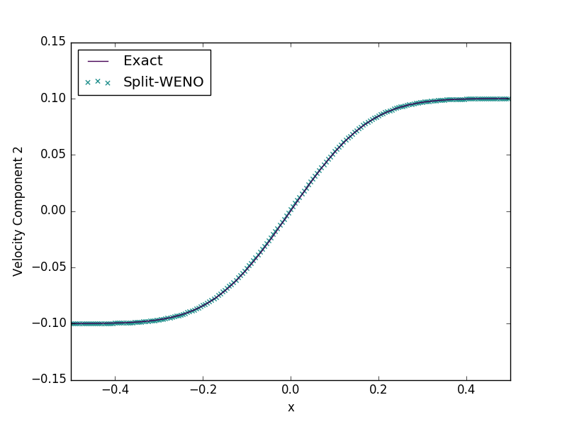
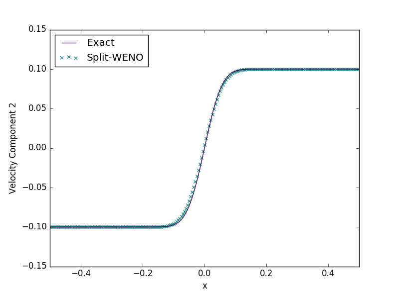
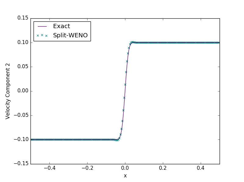
Figure 5: Results of solving Stokes’ First Problem ($\mu=10^{-2},\mu=10^{-3},\mu=10^{-4}$) with an ADER-WENO scheme and a Split-WENO scheme ($N=2$)

4.3 Viscous Shock

This test is designed to demonstrate that the numerical methods used are also able to cope with fast flows. First demonstrated by Becker Becker [3], the Navier-Stokes equations have an analytic solution for $P_{r}=0.75$ (see Johnson Johnson [17] for a full analysis). As noted by Dumbser Dumbser et al. [8], if the wave has nondimensionalised upstream velocity $\bar{v}=1$ and Mach number $M_{c}$, then its nondimensionalised downstream velocity is:

$$a=\frac{1+\frac{\gamma-1}{2}M_{c}^{2}}{\frac{\gamma+1}{2}M_{c}^{2}}$$ (82)

The wave’s velocity profile $\bar{v}\left(x\right)$ is given by the roots of the following equation:

$$\frac{1-\bar{v}}{\left(\bar{v}-a\right)^{a}} =c_{1}\exp\left(-c_{2}x\right)$$ (83a)

$$c_{1} =\left(\frac{1-a}{2}\right)^{1-a}$$ (83b)

$$c_{2} =\frac{3}{4}R_{e}\frac{M_{c}^{2}-1}{\gamma M_{c}^{2}}$$ (83c)

$c_{1},c_{2}$ are constants that affect the position of the center of the wave, and its stretch factor, respectively. Following the analysis of Morduchow and Libby Morduchow and Libby [21], the nondimensional pressure and density profiles are given by:

$$\bar{p}=\frac{1}{\bar{v}}\left(1+\frac{\gamma-1}{2}M_{c}^{2}\left(1-\bar{v}^{2}\right)\right)$$ (84)

$$\bar{\rho}=\frac{1}{\bar{v}}$$ (85)

To obtain an unsteady shock traveling into a region at rest, a constant velocity field $v=M_{c}c_{0}$ is imposed on the traveling wave solution presented here (where $c_{0}$ is the adiabatic sound speed). Thus, if $p_{0},\rho_{0}$ are the downstream (reference) values for pressure and density:

$$v =Mc_{0}\left(1-\bar{v}\right)$$ (86a)

$$p =p_{0}\bar{p}$$ (86b)

$$\rho =\rho_{0}\bar{\rho}$$ (86c)

These functions are used as initial conditions, along with $A=\sqrt[3]{\bar{\rho}}I$ and $\boldsymbol{J}=\boldsymbol{0}$. The downstream density and pressure are taken to be $\rho_{0}=1$ and $p_{0}=\frac{1}{\gamma}$ (so that $c_{0}=1$). $M_{c}=2$ and $R_{e}=100$. The material parameters are taken to be: $\gamma=1.4$, $p_{\infty}=0$, $c_{v}=2.5$, $c_{s}=5$, $\alpha=5$, $\mu=2\times 10^{-2}$, $\kappa=\frac{28}{3}\times 10^{-2}$ (resulting in $\tau_{1}=0.0048$, $\tau_{2}=0.00522\dot{6}$).

The results of a simulation with 200 cells at time $t=0.2$, using reconstruction polynomials of order $N=2$, are presented in Figure 6 on page 6 and Figure 7 on page 7. The shock was initially centered at $x=0.25$, reaching $x=0.65$ at the final time. Note that the density, velocity, and pressure results for both methods match the exact solution well, with the ADER-WENO method appearing to produce a slightly more accurate solution. The results for the two methods for the stress tensor and heat flux are close.

Figure 6: Density, velocity, and pressure for the Viscous Shock problem, solved with an ADER-WENO scheme and a Split-WENO scheme ($N=2$)

Figure 7: Viscous stress and heat flux for the Viscous Shock problem, solved with both an ADER-WENO scheme and a Split-WENO scheme ($N=2$)

4.4 Heat Conduction in a Gas

This is a simple test case to ensure that the heat transfer terms in the implementation are working correctly. Two ideal gases at different temperatures are initially in contact at position $x=0$. The initial conditions for this problem are given in Table 2 on page 2.

	$\rho$	$p$	$\boldsymbol{v}$	$A$	$\boldsymbol{J}$
$x<0$	$2$	$1$	$\boldsymbol{0}$	$\sqrt[3]{2}\cdot I_{3}$	$\boldsymbol{0}$
$x\geq 0$	$0.5$	$1$	$\boldsymbol{0}$	$\frac{1}{\sqrt[3]{2}}\cdot I_{3}$	$\boldsymbol{0}$

Table 2: Initial conditions for the heat conduction test

The material parameters are taken to be: $\gamma=1.4$, $c_{v}=2.5$, $\rho_{0}=1$, $p_{0}=1$, $c_{s}=1$, $\alpha=2$, $\mu=10^{-2}$, $\kappa=10^{-2}$ (resulting in $\tau_{1}=0.06$, $\tau_{2}=0.0025$). The results of a simulation with 200 cells at time $t=1$, using reconstruction polynomials of order $N=2$, are presented in Figure 8 on page 8. The ADER-WENO and Split-WENO methods are in perfect agreement for both the temperature and heat flux profiles. As demonstrated in Dumbser et al. [8], this means that they in turn agree very well with a reference Navier-Stokes-Fourier solution.

Figure 8: Results of solving the problem of Heat Conduction in Gas with both an ADER-WENO scheme and a Split-WENO scheme ($N=2$)

4.5 Speed

Both the ADER-WENO scheme and the Split-WENO scheme used in this study were implemented in Python3. All array functions were precompiled with Numba’s JIT capabilities and the root-finding procedure in the Galerkin predictor was performed using SciPy’s Newton-Krylov solver, compiled against the Intel MKL. Clear differences in computational cost between the ADER-WENO and Split-WENO methods were apparent, as is to be expected, owing to the lack of Galerkin method in the Split-WENO scheme. The wall times for the various tests undertaken in this study are given in Table 3 on page 3, comparing the combined WENO and Galerkin methods of the ADER-WENO scheme to the combined WENO and ODE methods of the Split-WENO scheme. All computations were performed using an Intel Core i7-4910MQ, on a single core. The number of time steps taken are given in Table 4 on page 4. The differences between the methods in terms of the number of time steps taken in each test result from the fact that, for numerical stability, CFL numbers of 0.8 and 0.7 were required by the ADER-WENO method and the Split-WENO method, respectively.

Note that, unlike with the ADER-WENO scheme, the wall time for the Split-WENO scheme is unaffected by a decrease in the viscosity in Stokes’ First Problem (and the corresponding increase in the stiffness of the source terms). This is because the analytic approximation to the distortion ODEs obviates the need for a stiff solver. The large difference in ADER-WENO solver times between the $\mu=10^{-3}$ and $\mu=10^{-4}$ cases is due to the fact that, in the latter case, a stiff solver must be employed for the initial guess to the root of the nonlinear system produced by the Discontinuous Galerkin method (as described in Hidalgo and Dumbser [15]).

	ADER-WENO	Split-WENO	Speed-up
Stokes’ First Problem ($\mu=10^{-2}$)	265s	38s	7.0
Stokes’ First Problem ($\mu=10^{-3}$)	294s	38s	7.7
Stokes’ First Problem ($\mu=10^{-4}$)	536s	38s	14.1
Viscous Shock	297s	56s	5.3
Heat Conduction in a Gas	544s	94s	5.8

Table 3: Wall time for various tests (all with 200 cells) under the ADER-WENO method and the Split-WENO method

	Timesteps (ADER-WENO)	Timesteps (Split-WENO)
Stokes’ First Problem ($\mu=10^{-2}$)	385	442
Stokes’ First Problem ($\mu=10^{-3}$)	386	443
Stokes’ First Problem ($\mu=10^{-4}$)	385	442
Viscous Shock	562	645
Heat Conduction in a Gas	942	1077

Table 4: Time steps taken for various tests (all with 200 cells) under the ADER-WENO method and the Split-WENO method

4.6 Convergence

To assess the rate of convergence of the Split-WENO method, the convected isentropic vortex convergence study from Dumbser et al. [8] was performed. The initial conditions are given as $\rho=1+\delta\rho$, $p=1+\delta p$, $\boldsymbol{v}=\left(1,1,0\right)+\delta\boldsymbol{v}$, $A=\sqrt[3]{\rho}I$, $\boldsymbol{J}=\boldsymbol{0}$, where:

$$\delta T =-\frac{\left(\gamma-1\right)\epsilon^{2}}{8\gamma\pi^{2}}e^{1-r^{2}}$$ (87a)

$$\delta\rho =\left(1+\delta T\right)^{\frac{1}{\gamma-1}}-1$$ (87b)

$$\delta p =\left(1+\delta T\right)^{\frac{\gamma}{\gamma-1}}-1$$ (87c)

$$\delta\boldsymbol{v} =\frac{\epsilon}{2\pi}e^{\frac{1-r^{2}}{2}}\left(\begin{array}[]{c}\begin{array}[]{c}-\left(y-5\right)\\ x-5\\ 0\end{array}\end{array}\right)$$ (87h)

The 2D domain is taken to be $\left[0,10\right]^{2}$. $\epsilon$ is taken to be 5. The material parameters are taken to be: $\gamma=1.4$, $c_{v}=2.5$, $\rho_{0}=1$, $p_{0}=1$, $c_{s}=0.5$, $\alpha=1$, $\mu=10^{-6}$, $\kappa=10^{-6}$ (resulting in $\tau_{1}=2.4\times 10^{-5}$, $\tau_{2}=10^{-6}$). Thus, this can be considered to be a stiff test case.

The convergence rates in the $L_{1}$, $L_{2}$, $L_{\infty}$ norms for the density variable are given in Table 5 on page 5 and Table 6 on page 6 for WENO reconstruction polynomial orders of $N=2$ and $N=3$, respectively. As expected, both sets of tests attain roughly second order convergence. For comparison, the corresponding results for this test from Dumbser et al. [8] - solved using a third-order P2P2 scheme - are given in Table 7 on page 7 for comparison.

Grid Size	$\epsilon\left(L_{1}\right)$	$\epsilon\left(L_{2}\right)$	$\epsilon\left(L_{\infty}\right)$	$\mathcal{O}\left(L_{1}\right)$	$\mathcal{O}\left(L_{2}\right)$	$\mathcal{O}\left(L_{\infty}\right)$
20	$2.87\times 10^{-3}$	$7.15\times 10^{-3}$	$6.21\times 10^{-2}$
40	$5.81\times 10^{-4}$	$1.62\times 10^{-3}$	$1.73\times 10^{-2}$	2.30	2.14	1.85
60	$1.98\times 10^{-4}$	$5.39\times 10^{-4}$	$5.94\times 10^{-3}$	2.65	2.70	2.63
80	$1.23\times 10^{-4}$	$3.47\times 10^{-4}$	$3.41\times 10^{-3}$	1.67	1.52	1.92

Table 5: Convergence rates for the Split-WENO method ($N=2$)

Grid Size	$\epsilon\left(L_{1}\right)$	$\epsilon\left(L_{2}\right)$	$\epsilon\left(L_{\infty}\right)$	$\mathcal{O}\left(L_{1}\right)$	$\mathcal{O}\left(L_{2}\right)$	$\mathcal{O}\left(L_{\infty}\right)$
10	$1.01\times 10^{-2}$	$2.58\times 10^{-2}$	$1.27\times 10^{-1}$
20	$1.68\times 10^{-3}$	$4.02\times 10^{-3}$	$2.93\times 10^{-2}$	2.59	2.68	2.11
30	$5.34\times 10^{-4}$	$1.57\times 10^{-3}$	$1.70\times 10^{-2}$	2.83	2.32	1.34
40	$3.32\times 10^{-4}$	$8.94\times 10^{-4}$	$7.55\times 10^{-3}$	1.65	1.95	2.82

Table 6: Convergence rates for the Split-WENO method ($N=3$)

Grid Size	$\epsilon\left(L_{1}\right)$	$\epsilon\left(L_{2}\right)$	$\epsilon\left(L_{\infty}\right)$	$\mathcal{O}\left(L_{1}\right)$	$\mathcal{O}\left(L_{2}\right)$	$\mathcal{O}\left(L_{\infty}\right)$
20	$9.44\times 10^{-3}$	$2.20\times 10^{-3}$	$2.16\times 10^{-3}$
40	$1.95\times 10^{-3}$	$4.50\times 10^{-4}$	$4.27\times 10^{-4}$	2.27	2.29	2.34
60	$7.52\times 10^{-4}$	$1.74\times 10^{-4}$	$1.48\times 10^{-4}$	2.35	2.35	2.61
80	$3.72\times 10^{-4}$	$8.66\times 10^{-5}$	$7.40\times 10^{-5}$	2.45	2.42	2.41

Table 7: Convergence rates for the ADER-DG PNPM method ($N,M=2$)

5 Conclusions

In summary, a new numerical method based on an operator splitting, and including some analytical results, has been proposed for the GPR model of continuum mechanics. It has been demonstrated that this method is able to match current ADER-WENO methods in terms of accuracy on a range of test cases. It is significantly faster than the other currently available methods, and it is easier to implement. The author would recommend that if very high order-of-accuracy is required, and computational cost is not important, then ADER-WENO methods may present a better option, as by design the new method cannot achieve better than second-order accuracy. This new method clearly has applications in which it will prove useful, however.

In a similar manner to the operator splitting method presented in Leveque and Yee [18], the Split-WENO method is second-order accurate and stable even for very stiff problems (in particular, the reader is referred to the results of the $\mu=10^{-4}$ variation of Stokes’ First Problem in 4.2 and the convergence study in 4.6). However, it will inevitably suffer from the incorrect speed of propagation of discontinuities on regular, structured grids. This is due to a lack of spatial resolution in evaluating the source terms, as detailed in Leveque and Yee [18]. This issue can be rectified by the use of some form of shock tracking or mesh refinement, as noted in the cited paper. It is noted in Dumbser et al. [6] that operator splitting-based methods can result in schemes that are neither well-balanced nor asymptotically consistent. The extent to which these two conditions are violated by the Split-WENO method - and the severity in practise of any potential violation - is a topic of further research.

It should be noted that the assumption (72) used to derive the approximate analytical solver may break down for situations where the flow is compressed heavily in one direction but not the others. The reason for this is that one of the singular values of the distortion tensor will be much larger than the others, and the mean of the squares of the singular values will not be close to its geometric mean, meaning that the subsequent linearization of the ODE governing the mean of the singular values fails. It should be noted that none of the situations covered in this study presented problems for the approximate analytical solver, and situations which may be problematic are in some sense unusual. In any case, a stiff ODE solver can be used to solve the system (54) if necessary, utilizing the Jacobians derived in the appendix, and so the Split-WENO method is still very much usable in these situations, albeit slightly slower.

It should be noted that both the ADER-WENO and Split-WENO methods, as described in this study, are trivially parallelizable on a cell-wise basis. Thus, given a large number of computational cores, deficiencies in the Split-WENO method in terms of its order of accuracy may be overcome by utilizing a larger number of computational cells and cores. The computational cost of each time step is significantly smaller than with the ADER-WENO method, and the number of grid cells that can be used scales roughly linearly with number of cores, at constant time per iteration.

6 References

7 Acknowledgments

I acknowledge financial support from the EPSRC Centre for Doctoral Training in Computational Methods for Materials Science under grant EP/L015552/1.

8 Appendix

8.1 Jacobian of Distortion ODEs

The Jacobian of the source function is used to speed up numerical integration of the ODE. It is derived thus:

$$\frac{\partial\operatorname{dev}\left(G\right)_{ij}}{\partial A_{mn}}=\delta_{in}A_{mj}+\delta_{jn}A_{mi}-\frac{2}{3}\delta_{ij}A_{mn}$$ (88)

Thus:

$$\frac{\partial\left(A\operatorname{dev}\left(G\right)\right)_{ij}}{\partial A_{mn}} =\frac{\partial A_{it}}{\partial A_{mn}}\operatorname{dev}\left(G\right)_{tj}+A_{it}\frac{\partial\operatorname{dev}\left(G\right)_{tj}}{\partial A_{mn}}$$ (89)

$$=\delta_{im}\delta_{tn}\left(A_{kt}A_{kj}-\frac{1}{3}A_{kl}A_{kl}\delta_{tj}\right)+A_{it}\left(\delta_{tn}A_{mj}+\delta_{jn}A_{mt}-\frac{2}{3}\delta_{tj}A_{mn}\right)$$

$$=\delta_{im}A_{kn}A_{kj}-\frac{1}{3}\delta_{im}\delta_{jn}A_{kl}A_{kl}+A_{in}A_{mj}+\delta_{jn}A_{ik}A_{mk}-\frac{2}{3}A_{ij}A_{mn}$$

Thus:

$$J_{A} \equiv\frac{-3}{\tau_{1}}\frac{\partial\left(\det\left(A\right)^{\frac{5}{3}}A\operatorname{dev}\left(G\right)\right)_{ij}}{\partial A_{mn}}$$ (90)

$$=\frac{-3}{\tau_{1}}\det\left(A\right)^{\frac{5}{3}}\left(\frac{5}{3}\left(A\operatorname{dev}\left(G\right)\right)_{ij}A_{mn}^{-T}+A_{in}A_{mj}+\delta_{jn}G_{im}^{{}^{\prime}}+\delta_{im}G_{jn}-\frac{1}{3}\delta_{im}\delta_{jn}A_{kl}A_{kl}-\frac{2}{3}A_{ij}A_{mn}\right)$$

$$=\frac{1}{\tau_{1}}\det\left(A\right)^{\frac{5}{3}}\left(-5\left(A\operatorname{dev}\left(G\right)\right)\otimes A^{-T}+2A\otimes A-3\left(A\otimes A\right)^{1,3}+\left\|A\right\|_{F}^{2}\left(I\otimes I\right)^{2,3}-3\left(G^{{}^{\prime}}\otimes I+I\otimes G\right)^{2,3}\right)$$

where $G^{{}^{\prime}}=AA^{T}$ and $X^{a,b}$ refers to tensor $X$ with indices $a,b$ transposed.

8.2 Jacobian of Thermal Impulse ODEs

As demonstrated in 3.1, we have:

$$\frac{dJ_{i}}{dt}=\frac{J_{i}}{2}\left(-a+b\left(J_{1}^{2}+J_{2}^{2}+J_{3}^{2}\right)\right)$$ (91)

where

$$a =\frac{2\rho_{0}}{\tau_{2}T_{0}\rho c_{v}}\left(E-E_{2A}\left(A\right)-E_{3}\left(\boldsymbol{v}\right)\right)$$ (92a)

$$b =\frac{\rho_{0}\alpha^{2}}{\tau_{2}T_{0}\rho c_{v}}$$ (92b)

Thus, the Jacobian of the thermal impulse ODEs is:

$$\left(\begin{array}[]{ccc}\frac{b}{2}\left(3J_{1}^{2}+J_{2}^{2}+J_{3}^{2}\right)-\frac{a}{2}&bJ_{1}J_{2}&bJ_{1}J_{3}\\ bJ_{1}J_{2}&\frac{b}{2}\left(J_{1}^{2}+3J_{2}^{2}+J_{3}^{2}\right)-\frac{a}{2}&bJ_{2}J_{3}\\ bJ_{1}J_{3}&bJ_{2}J_{3}&\frac{b}{2}\left(J_{1}^{2}+J_{2}^{2}+3J_{3}^{2}\right)-\frac{a}{2}\end{array}\right)$$ (93)

8.3 WENO Matrices for $N=2$

$$M_{1} =\left(\begin{array}[]{ccc}2\sqrt{\frac{5}{3}}+\frac{245}{18}&-\frac{236}{9}&\frac{245}{18}-2\sqrt{\frac{5}{3}}\\ \sqrt{\frac{5}{3}}+\frac{65}{18}&-\frac{56}{9}&\frac{65}{18}-\sqrt{\frac{5}{3}}\\ \frac{5}{18}&\frac{4}{9}&\frac{5}{18}\end{array}\right)$$ (94d)

$$M_{2} =\left(\begin{array}[]{ccc}\sqrt{\frac{5}{3}}+\frac{65}{18}&-\frac{56}{9}&\frac{65}{18}-\sqrt{\frac{5}{3}}\\ \frac{5}{18}&\frac{4}{9}&\frac{5}{18}\\ \frac{65}{18}-\sqrt{\frac{5}{3}}&-\frac{56}{9}&\sqrt{\frac{5}{3}}+\frac{65}{18}\end{array}\right)$$ (94h)

$$M_{3} =\left(\begin{array}[]{ccc}\frac{5}{18}&\frac{4}{9}&\frac{5}{18}\\ \frac{65}{18}-\sqrt{\frac{5}{3}}&-\frac{56}{9}&\sqrt{\frac{5}{3}}+\frac{65}{18}\\ \frac{245}{18}-2\sqrt{\frac{5}{3}}&-\frac{236}{9}&2\sqrt{\frac{5}{3}}+\frac{245}{18}\end{array}\right)$$ (94l)

$$M_{1}^{-1} =\left(\begin{array}[]{ccc}\frac{1}{60}\left(2-3\sqrt{15}\right)&\sqrt{\frac{3}{5}}-\frac{1}{15}&\frac{1}{60}\left(62-9\sqrt{15}\right)\\ -\frac{1}{24}&\frac{1}{12}&\frac{23}{24}\\ \frac{1}{60}\left(3\sqrt{15}+2\right)&-\sqrt{\frac{3}{5}}-\frac{1}{15}&\frac{1}{60}\left(9\sqrt{15}+62\right)\end{array}\right)$$ (95d)

$$M_{2}^{-1} =\left(\begin{array}[]{ccc}\frac{1}{60}\left(3\sqrt{15}+2\right)&\frac{14}{15}&\frac{1}{60}\left(2-3\sqrt{15}\right)\\ -\frac{1}{24}&\frac{13}{12}&-\frac{1}{24}\\ \frac{1}{60}\left(2-3\sqrt{15}\right)&\frac{14}{15}&\frac{1}{60}\left(3\sqrt{15}+2\right)\end{array}\right)$$ (95h)

$$M_{3}^{-1} =\left(\begin{array}[]{ccc}\frac{1}{60}\left(9\sqrt{15}+62\right)&-\sqrt{\frac{3}{5}}-\frac{1}{15}&\frac{1}{60}\left(3\sqrt{15}+2\right)\\ \frac{23}{24}&\frac{1}{12}&-\frac{1}{24}\\ \frac{1}{60}\left(62-9\sqrt{15}\right)&\sqrt{\frac{3}{5}}-\frac{1}{15}&\frac{1}{60}\left(2-3\sqrt{15}\right)\end{array}\right)$$ (95l)

References

• Balsara et al. [2009] Balsara, D. S., Rumpf, T., Dumbser, M., Munz, C. D., 2009. Efficient, high accuracy ADER-WENO schemes for hydrodynamics and divergence-free magnetohydrodynamics. Journal of Computational Physics 228 (7), 2480–2516.
URL http://dx.doi.org/10.1016/j.jcp.2008.12.003
• Barton and Drikakis [2010] Barton, P. T., Drikakis, D., 2010. An Eulerian method for multi-component problems in non-linear elasticity with sliding interfaces. Journal of Computational Physics 229 (15), 5518–5540.
URL http://dx.doi.org/10.1016/j.jcp.2010.04.012
• Becker [1929] Becker, R., 1929. Impact Waves and Detonation. Zeitschrift für Physik 8, 381.
• Boscheri et al. [2016] Boscheri, W., Dumbser, M., Loubère, R., 2016. Cell centered direct Arbitrary-Lagrangian-Eulerian ADER-WENO finite volume schemes for nonlinear hyperelasticity. Computers and Fluids 134-135, 111–129.
• Dumbser et al. [2008a] Dumbser, M., Balsara, D. S., Toro, E. F., Munz, C. D., 2008a. A unified framework for the construction of one-step finite volume and discontinuous Galerkin schemes on unstructured meshes. Journal of Computational Physics 227 (18), 8209–8253.
• Dumbser et al. [2008b] Dumbser, M., Enaux, C., Toro, E. F., 2008b. Finite volume schemes of very high order of accuracy for stiff hyperbolic balance laws. Journal of Computational Physics 227 (8), 3971–4001.
• Dumbser et al. [2014] Dumbser, M., Hidalgo, A., Zanotti, O., 2014. High order space-time adaptive ADER-WENO finite volume schemes for non-conservative hyperbolic systems. Computer Methods in Applied Mechanics and Engineering 268, 359–387.
• Dumbser et al. [2016] Dumbser, M., Peshkov, I., Romenski, E., Zanotti, O., 2016. High order ADER schemes for a unified first order hyperbolic formulation of continuum mechanics: Viscous heat-conducting fluids and elastic solids. Journal of Computational Physics 314, 824–862.
URL http://arxiv.org/abs/1511.08995
• Dumbser and Toro [2011a] Dumbser, M., Toro, E. F., 2011a. A simple extension of the Osher Riemann solver to non-conservative hyperbolic systems. Journal of Scientific Computing 48 (1-3), 70–88.
• Dumbser and Toro [2011b] Dumbser, M., Toro, E. F., 2011b. On universal Osher-type schemes for general nonlinear hyperbolic conservation laws. Communications in Computational Physics 10 (3), 635–671.
• Dumbser et al. [2013] Dumbser, M., Zanotti, O., Hidalgo, A., Balsara, D. S., 2013. ADER-WENO finite volume schemes with space-time adaptive mesh refinement. Journal of Computational Physics 248, 257–286.
• Frenkel [1947] Frenkel, J., 1947. Kinetic Theory of Liquids. Oxford University Press.
• Giles [2008] Giles, M. B., 2008. An extended collection of matrix derivative results for forward and reverse mode algorithmic differentiation. Tech. rep., University of Oxford.
URL http://eprints.maths.ox.ac.uk/1079/
• Godunov and Romenski [2003] Godunov, S. K., Romenski, E., 2003. Elements of continuum mechanics and conservation laws.
• Hidalgo and Dumbser [2011] Hidalgo, A., Dumbser, M., 2011. ADER schemes for nonlinear systems of stiff advection-diffusion-reaction equations. Journal of Scientific Computing 48 (1-3), 173–189.
• Jackson [2017] Jackson, H., 2017. On the Eigenvalues of the ADER-WENO Galerkin Predictor. Journal of Computational Physics 333 (March 2017), 409–413.
URL http://dx.doi.org/10.1016/j.jcp.2016.12.058
• Johnson [2013] Johnson, B. M., 2013. Analytical shock solutions at large and small Prandtl number. Journal of Fluid Mechanics 726, 1–12.
URL http://adsabs.harvard.edu/abs/2013arXiv1305.7132J
• Leveque and Yee [1990] Leveque, R., Yee, H., 1990. A Study of Numerical Methods for Hyperbolic Conservation Laws with Stiff Source Terms. Journal of Computational Physics 86, 187–210.
• Malyshev and Romenskii [1986] Malyshev, A. N., Romenskii, E. I., 1986. Hyperbolic equations for heat transfer. Global solvability of the Cauchy problem. Siberian Mathematical Journal 27 (5), 734–740.
• McAdams et al. [2011] McAdams, A., Selle, A., Tamstorf, R., Teran, J., Sifakis, E., 2011. Computing the Singular Value Decomposition of 3 x 3 matrices with minimal branching and elementary floating point operations. University of Wisconsin Madison.
• Morduchow and Libby [1949] Morduchow, M., Libby, P. A., 1949. On a Complete Solution of the One-Dimensional Flow Equations of a Viscous, Heat-Conducting, Compressible Gas. Tech. rep., Polytechnic Institute of Brooklyn.
• Oliphant [2007] Oliphant, T. E., 2007. SciPy: Open source scientific tools for Python.
URL http://www.scipy.org/
• Peshkov and Romenski [2016] Peshkov, I., Romenski, E., 2016. A hyperbolic model for viscous Newtonian flows. Continuum Mechanics and Thermodynamics 28 (1-2), 85–104.
• Romenski et al. [2010] Romenski, E., Drikakis, D., Toro, E., 2010. Conservative models and numerical methods for compressible two-phase flow. Journal of Scientific Computing 42 (1), 68–95.
• Romenski et al. [2007] Romenski, E., Resnyansky, A. D., Toro, E. F., 2007. Conservative hyperbolic model for compressible two-phase flow with different phase pressures and temperatures. Quarterly of applied mathematics 65(2) (2), 259–279.
• Romenski [1989] Romenski, E. I., 1989. Hyperbolic equations of Maxwell’s nonlinear model of elastoplastic heat-conducting media. Siberian Mathematical Journal 30 (4), 606–625.
• Toro [2009] Toro, E., 2009. Riemann solvers and numerical methods for fluid dynamics: a practical introduction. Springer.
• Zanotti and Dumbser [2016] Zanotti, O., Dumbser, M., 2016. Efficient conservative ADER schemes based on WENO reconstruction and space-time predictor in primitive variables. Computational Astrophysics and Cosmology 3 (1), 1.
URL http://www.comp-astrophys-cosmol.com/content/3/1/1