Robust Stability of Optimization-based State Estimation

Abstract

Optimization-based state estimation is useful for nonlinear or constrained dynamic systems for which few general methods with established properties are available. The two fundamental forms are moving horizon estimation (MHE) which uses the nearest measurements within a moving time horizon, and its theoretical ideal, full information estimation (FIE) which uses all measurements up to the time of estimation. Despite extensive studies, the stability analyses of FIE and MHE for discrete-time nonlinear systems with bounded process and measurement disturbances, remain an open challenge. This work aims to provide a systematic solution for the challenge. First, we prove that FIE is robustly globally asymptotically stable (RGAS) if the cost function admits a property mimicking the incremental input/output-to-state stability (i-IOSS) of the system and has a sufficient sensitivity to the uncertainty in the initial state. Second, we establish an explicit link from the RGAS of FIE to that of MHE, and use it to show that MHE is RGAS under enhanced conditions if the moving horizon is long enough to suppress the propagation of uncertainties. The theoretical results imply flexible MHE designs with assured robust stability for a broad class of i-IOSS systems. Numerical experiments on linear and nonlinear systems are used to illustrate the designs and support the findings.

I Introduction

Optimization-based state estimation refers to an estimation method that estimates the state of a system via an optimization approach, in which the optimization utilizes all or a subset of the information available about the system up to the time of estimation. It has advantages in handling nonlinear or constrained systems for which few general state estimation methods with established properties are available [1]. Full information estimation (FIE) is an ideal form of optimization-based estimation which uses all measurements up to the time of estimation. In the absence of constraints, FIE is equivalent to Kalman filtering (KF) when the system is linear time-invariant and the cost function has an appropriate quadratic form [1]. Since the measurements increase with time, it is impractical to implement FIE. This motivates the development of moving horizon estimation (MHE) as its practical approximation which uses only the latest batch of measurements to do the estimation. The idea of MHE dates back to 1960’s [2] which was motivated for making KF robust to modeling errors. However, it is not until recently that the idea is gradually developed into a field, i.e., the field of MHE [3, 4, 5, 1]. The recent developments include MHE theoretical and applied researches which investigate the stability and the implementation issues of MHE.

Theoretical research has been concentrated on the stability conditions of MHE. Early research assumed linear systems [6, 7, 8], and later nonlinear systems [9, 10, 11, 12]. Part of the stability results were obtained by assuming the presence of measurement disturbances but the absence of process disturbances, e.g., [10], and most were obtained by assuming the presence of both disturbances, e.g., [6, 9, 7, 11, 8, 12]. And the stability results were derived based on different formulations of the problems. For example, references [6, 7, 8, 13, 14] considered either linear or nonlinear systems and each assumed a quadratic cost function that accounts for a quadratic arrival cost and quadratic penalties on the measurement fitting errors. Whereas, references [11, 5, 15, 16, 17] considered general nonlinear systems and assumed a general form of cost functions that are not necessarily in a quadratic form.

The recent review made in [5] provides a concise and general view of the problem which relies on the concept of incremental input/output-to-state stability (i-IOSS; refer to Definition 2 in Section II) for detectability of nonlinear systems [18] and the concept of robust global asymptotic stability (RGAS) for robust stability of a state estimator [19, 5]. The review revealed two major challenges that were open in the field [5, 1]: (i) the search for conditions and a proof of the RGAS of MHE in the presence of bounded disturbances, and (ii) the development of suboptimal MHE that enables an efficient computation of the solution. As an initial step to tackling challenge (i), reference [15] identified a broad class of cost functions that ensure the RGAS of FIE, and the cost functions were shown to admit a more specific form for a class of i-IOSS systems considered in [16]. The implication to the RGAS of MHE was further investigated in [17] based on the results of [16], which showed that MHE is RGAS if the same conditions are enhanced properly. Moreover, in [17] the convergence of MHE for convergent disturbances was proved under the enhanced conditions, and the MHE was shown to be RGAS even if the cost function does not have max terms which are needed in the stability analyses of FIE [16].

Other relevant progress was reported in [14], which assumed a quadratic cost function and used a nonlinear deterministic observer to generate useful constraints so that the MHE results in bounded estimation errors under certain conditions. Some earlier developments are also available in [12, 13], which assumed a quadratic cost function for MHE and also an observability and some Lipschitz conditions on the system. The other developments of MHE are mainly in applied research, which mostly aimed at reducing the online computational complexity of MHE for applications in large dimensional and nonlinear systems [1]. Interested readers are referred to [20, 21, 22, 23, 24] and the references therein for relevant examples.

This paper follows the general view of MHE developed in [5], and aims to present a systematic solution for the aforementioned open challenge (i). It significantly extends our conference paper [15], which identified sufficient conditions for the RGAS of FIE. The major new contributions are the following. First, an explicit link is established from the RGAS of FIE to that of MHE. Second, based on the link we prove the RGAS of MHE under both general and specialized conditions, depending on the stability property of a system. The convergence of MHE to the true state is also established for a system subjected to disturbances that converge to zero. Third, two numerical examples are developed with rigorous analyses to support the theoretical findings. The numerical results are compared with those obtained by KF in the linear case and extended Kalman filter (EKF) [25] in the nonlinear case, demonstrating the advantages of MHE in the considered situations.

Since the discrete-time system and the MHE are assumed to have general forms, the theoretical results imply flexible MHE designs with assured robust stability for a broad class of systems. This constitutes a key difference from the recent stability results obtained in [17] which are applicable to a subset of the considered systems.

The rest of the paper is organized as follows. Section II introduces the notation and some preliminaries. Section III defines the ideal and the practical forms of optimization-based state estimation, i.e., FIE and MHE. Section IV proves the robust stability of FIE under general and then specialized conditions. Section V reveals its implication to MHE and subsequently proves the robust stability of MHE under enhanced conditions. Convergence of the MHE is also proved for disturbances that are convergent to zero. Section VI presents two numerical examples to illustrate the flexible MHE designs. Section VII provides a brief discussion on ways to tackle the computational challenge of MHE. Finally, Section VIII concludes the paper with a remark on the future work.

II Notation and Preliminaries

The notation mostly follows the convention in [5]. The symbols $\mathbb{R}$, $\mathbb{R}_{\geq 0}$ and $\mathbb{I}_{\geq 0}$ denote the sets of real numbers, nonnegative real numbers and nonnegative integers, respectively, and $\mathbb{I}_{a:b}$ denotes the set of integers from $a$ to $b$. The constraints $t\geq 0$ and $t\in\mathbb{I}_{\geq 0}$ are used interchangeably to refer to the set of discrete times. The symbol $\left|\cdot\right|$ denotes the Euclidean norm of a vector or the 2-norm of a matrix, depending on the argument. The bold symbol $\boldsymbol{x}_{a:b}$, denotes a sequence of vector-valued variables $\{x_{a},\,x_{a+1},\,...,\thinspace x_{b}\}$, and with a function $f$ acting on a vector $x$, $f(\boldsymbol{x}_{a:b})$ stands for the sequence of function values $\{f(x_{a}),\,f(x_{a+1}),\,...,\thinspace f(x_{b})\}$. The notation $\left\|\boldsymbol{x}_{a:b}\right\|$ refers to $\max_{a\leq i\leq b}\left|x_{i}\right|$ if $a\leq b$ and to 0 if $a>b$. Throughout the paper, $t$ refers to a discrete time, and as a subscript it indicates dependence on time $t$. Whereas, the subscripts or superscripts $x$, $w$ and $v$ are used exclusively to indicate a function or variable that is associated with the state ($x$), disturbance ($w$) or measurement noise ($v$), and they do not imply dependence relationships. The frequently used $\mathcal{K}$, $\mathcal{K}_{\infty}$, $\mathcal{L}$ and $\mathcal{KL}$ functions are defined as follows.

Definition 1.

($\mathcal{K}$, $\mathcal{K}_{\infty}$, $\mathcal{L}$ and $\mathcal{KL}$ functions) A function $\alpha:\mathbb{R}_{\geq 0}\to\mathbb{R}_{\geq 0}$ is a $\mathcal{K}$ function if it is continuous, zero at zero, and strictly increasing, and a $\mathcal{K}_{\infty}$ function if $\alpha$ is a $\mathcal{K}$ function and satisfies $\alpha(s)\to\infty$ as $s\to\infty$. A function $\varphi:\mathbb{R}_{\geq 0}\to\mathbb{R}_{\geq 0}$ is a $\mathcal{L}$ function if it is continuous, nonincreasing and satisfies $\varphi(t)\to 0$ as $t\to\infty$. A function $\beta:\mathbb{R}_{\geq 0}\times\mathbb{R}_{\geq 0}\to\mathbb{R}_{\geq 0}$ is a $\mathcal{KL}$ function if, for each $t\geq 0$, $\beta(\cdot,t)$ is a $\mathcal{K}$ function and for each $s\geq 0$, $\beta(s,\cdot)$ is a $\mathcal{L}$ function.

The following properties of the $\mathcal{K}$ and $\mathcal{KL}$ functions will be used in later analyses.

Lemma 1.

[26, 5] Given a $\mathcal{K}$ function $\alpha$ and a $\mathcal{KL}$ function $\beta$, the following holds for all $a_{i}\in\mathbb{R}_{\geq 0}$, $i\in\mathbb{I}_{1:n}$, and all $t\in\mathbb{R}_{\geq 0}$,

$$\alpha\left(\sum_{i=1}^{n}a_{i}\right)\leq\sum_{i=1}^{n}\alpha(na_{i}),\,\,\beta\left(\sum_{i=1}^{n}a_{i},t\right)\leq\sum_{i=1}^{n}\beta(na_{i},t).$$

Definition 2.

(i-IOSS [5, 18]) The system $x_{t+1}=f(x_{t},w_{t})$, $y_{t}=h(x_{t})$ is i-IOSS if there exist functions $\beta\in\mathcal{KL}$ and $\alpha_{1},\alpha_{2}\in\mathcal{K}$ such that for every two initial states $x_{0}^{(1)},x_{0}^{(2)}$, and two sequences of disturbances $\boldsymbol{w}_{0:t-1}^{(1)},\boldsymbol{w}_{0:t-1}^{(2)}$, the following inequality holds for all $t\in\mathbb{I}_{\geq 0}$:

$$\left|x_{t}(x_{0}^{(1)},\boldsymbol{w}_{0:t-1}^{(1)})-x_{t}(x_{0}^{(2)},\boldsymbol{w}_{0:t-1}^{(2)})\right|\leq\beta(\left|x_{0}^{(1)}-x_{0}^{(2)}\right|,t)$$

$$+\alpha_{1}(\left\|\boldsymbol{w}_{0:t-1}^{(1)}-\boldsymbol{w}_{0:t-1}^{(2)}\right\|)+\alpha_{2}(\left\|h(\boldsymbol{x}_{0:t}^{(1)})-h(\boldsymbol{x}_{0:t}^{(2)})\right\|),$$ (1)

where $x_{t}^{(i)}$ is a shorthand of $x_{t}(x_{0}^{(i)},\boldsymbol{w}_{0:t-1}^{(i)})$ for $i=1$ and 2.

The definition of i-IOSS can be interpreted as a “detectability” concept for nonlinear systems [18], as the state may be “detected” from the noise-free output by (1).

In particular, if in (1) $\beta(s,t)=\alpha(s)a^{t}$ for all $s,t\geq 0$, with $\alpha\in\mathcal{K}$ and $a$ being a constant within $(0,1)$, we say that the system is exponentially i-IOSS or exp-i-IOSS for short. This can be viewed as extending the exponential input-to-state stability [27, 28] to the context of i-IOSS.

Definition 3.

($\mathcal{K\cdot L}$ function) A $\mathcal{KL}$ function $\beta$ is called a $\mathcal{K\cdot L}$ function if there exist functions $\alpha\in\mathcal{K}$ and $\varphi\in\mathcal{L}$ such that $\beta(s,t)=\alpha(s)\varphi(t)$, for all $s,t\geq 0$.

As an example, the $\mathcal{KL}$ function $se^{-t}$ is a $\mathcal{K\cdot L}$ function for $s,t\geq 0$. The next lemma shows the general interest of a $\mathcal{K\cdot L}$ function.

Lemma 2.

($\mathcal{K\cdot L}$ bound, Lemma 8 in [29]) Given an arbitrary $\mathcal{KL}$ function $\beta$, there exists a $\mathcal{K\cdot L}$ function $\bar{\beta}$ such that $\beta(s,t)\leq\bar{\beta}(s,t)$ for all $s,t\geq 0$.

Lemma 2 implies that the i-IOSS property defined by means of a $\mathcal{KL}$ function can be defined equivalently using a $\mathcal{K\cdot L}$ function. This is useful in the later analyses of FIE and MHE. The following definition of a Lipschitz continuous function will also be used in the analysis of MHE.

Definition 4.

(Lipschitz continuous function) A function $f:\mathbb{R}^{n}\to\mathbb{R}^{m}$ is Lipschitz continuous over a subset $\mathbb{S}\in\mathbb{R}^{n}$ if there is a constant $c$ such that $|f(x)-f(y)|\leq c|x-y|$ for all $x,\thinspace y\in\mathbb{S}$.

III Optimization-based State Estimation

Consider a discrete-time nonlinear system described by

$$x_{t+1}=f(x_{t},w_{t}),\,\,y_{t}=h(x_{t})+v_{t},$$ (2)

where $x_{t}\in\mathbb{R}^{n}$ is the system state, $y_{t}\in\mathbb{R}^{p}$ the measurement, $w_{t}\in\mathbb{R}^{g}$ the process disturbance, $v_{t}\in\mathbb{R}^{p}$ the measurement disturbance, all at time $t$.

Since control inputs known up to the estimation time can be treated as given constants, they do not cause difficulty to the later defined optimization and related analyses and hence are ignored for brevity in the problem formulation [5]. The functions $f$ and $h$ are assumed to be continuous and known, and the initial state $x_{0}$ and the disturbances $(w_{t},v_{t})$ are modeled as unknown but bounded variables.

Given a time $t$, the state estimation problem is to find an optimal estimate of state $x_{t}$ based on measurements $\{y_{\tau}\}$ for $\tau$ belonging to a time set and satisfying $\tau\leq t$. In the ideal case, all measurements up to time $t$ are used, leading to the so-called FIE; and in the practical case, only measurements within a limited distance from time $t$ are used, yielding the so-called MHE. Both FIE and MHE can be cast as optimization problems as defined next.

Let the decision variables of FIE be $(\boldsymbol{\chi}_{0:t},\boldsymbol{\omega}_{0:t-1},\boldsymbol{\nu}_{0:t})$, which correspond to the system variables $(\boldsymbol{x}_{0:t},\boldsymbol{w}_{0:t-1},\boldsymbol{v}_{0:t})$, and the optimal decision variables be $(\hat{\boldsymbol{x}}_{0:t},\hat{\boldsymbol{w}}_{0:t-1},\hat{\boldsymbol{v}}_{0:t})$. Since $\hat{\boldsymbol{x}}_{0:t}$, which consists of optimal estimates at all sampled times, is uniquely determined once $\hat{x}_{0}$ and $\hat{\boldsymbol{w}}_{0:t-1}$ are known, the decision variables essentially reduce to $(\boldsymbol{\chi}_{0},\boldsymbol{\omega}_{0:t-1},\boldsymbol{\nu}_{0:t})$.

Here, although $\boldsymbol{\nu}_{0:t}$ is uniquely determined by $\boldsymbol{\chi}_{0}$ and $\boldsymbol{\omega}_{0:t-1}$, we keep it for the convenience of expressing bounds and penalty costs to be defined on $\boldsymbol{\nu}_{0:t}$.

Given a present time $t\in\mathbb{I}_{\geq 0}$, let $\bar{x}_{0}$ be the prior estimate of the initial state which may be obtained from the initial or historical measurements. The uncertainty in the initial state is thus represented by $\chi_{0}-\bar{x}_{0}$. Denote the time-dependent cost function as $V_{t}(\chi_{0}-\bar{x}_{0},\boldsymbol{\omega}_{0:t-1},\boldsymbol{\nu}_{0:t})$, which penalizes uncertainties in the initial state, the process and the measurements. Then, FIE is defined by the following optimization problem:

$$\mathrm{FIE:} \inf V_{t}(\chi_{0}-\bar{x}_{0},\boldsymbol{\omega}_{0:t-1},\boldsymbol{\nu}_{0:t})$$ (3)

$$\mathrm{subject~{}to,~{}} \chi_{\tau+1}=f(\chi_{\tau},\omega_{\tau}),\,\,\forall\tau\in\mathbb{I}_{0:t-1},$$

$$y_{\tau}=h(\chi_{\tau})+\nu_{\tau},\,\,\forall\tau\in\mathbb{I}_{0:t},$$

$$\chi_{0}\in\mathbb{B}_{x}^{0},\thinspace\thinspace\boldsymbol{\omega}_{0:t-1}\in\mathbb{B}_{w}^{0:t-1},\,\,\boldsymbol{\nu}_{0:t}\in\mathbb{B}_{v}^{0:t},$$

where $\{\chi_{0},\thinspace\boldsymbol{\omega}_{0:t-1},\thinspace\boldsymbol{\nu}_{0:t}\}$ are the decision variables. Here $\mathbb{B}_{x}^{0}$, $\mathbb{B}_{w}^{0:t-1}$ and $\mathbb{B}_{v}^{0:t}$ denote the sets of bounded initial states, bounded sequences of process and measurement disturbances, respectively, for all $t\in\mathbb{I}_{\geq 0}$, of which the latter two sets may vary with time. Since the optimal decision variable $\hat{x}_{\tau}$, for any $\tau\leq t$, is dependent on the time $t$ when the FIE instance is defined, to be unambiguous we use $\hat{x}_{t}^{*}$ to exclusively represent $\hat{x}_{t}$ that is obtained from the FIE instance defined at time $t$. This keeps $\hat{x}_{t}^{*}$ unique, while $\hat{x}_{t}$ varies as the FIE is renewed with new measurements as time elapses.

Given a constant $T\in\mathbb{I}_{\geq 0}$, if the measurements are limited only to the $T+1$ measurements backwards from and including the present time $t$, then the following optimization defines MHE, i.e.,

$$\mathrm{MHE:~{}} \inf V_{T}(\chi_{t-T}-\bar{x}_{t-T},\boldsymbol{\omega}_{t-T:t-1},\boldsymbol{\nu}_{t-T:t})$$ (4)

$$\mathrm{subject~{}to,~{}} \chi_{\tau+1}=f(\chi_{\tau},\omega_{\tau}),\,\,\forall\tau\in\mathbb{I}_{t-T:t-1},$$

$$y_{\tau}=h(\chi_{\tau})+\nu_{\tau},\,\,\forall\tau\in\mathbb{I}_{t-T:t},$$

$$\boldsymbol{\chi}_{t-T}\in\mathbb{B}_{x}^{t-T}, \boldsymbol{\omega}_{t-T:t-1}\in\mathbb{B}_{w}^{t-T:t-1},\,\,\boldsymbol{\nu}_{t-T:t}\in\mathbb{B}_{v}^{t-T:t},$$

where $\{\chi_{t-T},\thinspace\boldsymbol{\omega}_{t-T:t-1},\thinspace\boldsymbol{\nu}_{t-T:t}\}$ are the decision variables, and $\bar{x}_{t-T}$ is a prior estimate of $x_{t-T}$, and $\mathbb{B}_{x}^{t-T}$, $\mathbb{B}_{w}^{t-T:t-1}$ and $\mathbb{B}_{v}^{t-T:t}$ denote the bounding sets for the time period from $t-T$ to $t$. We use $\hat{x}_{t}^{\star}$ to represent $\hat{x}_{t}$ that is obtained from the MHE instance defined at time $t$. By this way, $\hat{x}_{t}^{\star}$ remains unique although $\hat{x}_{t}$ varies as the MHE instance is renewed with new measurements. Since the cost function is in the same form of FIE except for the truncated argument variables, the MHE defined in (4) is named as the associated MHE of the FIE defined in (3), and vice versa.

By definition, FIE uses all available historical measurements to perform state estimation. So its computational complexity increases with time and will ultimately become intractable, which makes FIE impractical for applications. For this reason, FIE is studied mainly for its theoretical interest: its performance can be viewed as a limit or benchmark that MHE tries to approach, and its stability can be a good start point for the stability analysis of MHE, which will become clear later on.

An important issue in designing FIE and MHE is to identify conditions under which the associated optimizations have optimal solutions such that the state estimates satisfy the RGAS property defined below. Let $\boldsymbol{x}_{0:t}(x_{0},\boldsymbol{w}_{0:t-1})$ denote a state sequence generated from an initial condition $x_{0}$, and a disturbance sequence $\boldsymbol{w}_{0:t-1}$.

Definition 5.

(RGAS [5]) The estimate $\hat{x}_{t}$ of the state $x_{t}$ is based on partial or full sequence of the noisy measurements, $\boldsymbol{y}_{0:t}=h(\boldsymbol{x}_{0:t}(x_{0},\boldsymbol{w}_{0:t-1}))+\boldsymbol{v}_{0:t}$. The estimate is RGAS if for all $x_{0}$ and $\bar{x}_{0}$, there exist functions $\beta_{x}\in\mathcal{KL}$ and $\alpha_{w},\alpha_{v}\in\mathcal{K}$ such that the following inequality holds for all $\boldsymbol{\omega}_{0:t-1}\in\mathbb{B}_{w}^{0:t-1}$, $\boldsymbol{\nu}_{0:t}\in\mathbb{B}_{v}^{0:t}$ and $t\in\mathbb{I}_{\geq 0}$:

$$\left|x_{t}-\hat{x}_{t}\right|$$

$$\leq\beta_{x}(\left|x_{0}-\bar{x}_{0}\right|,t)+\alpha_{w}(\left\|\boldsymbol{w}_{0:t-1}\right\|)+\alpha_{v}(\left\|\boldsymbol{v}_{0:t}\right\|).$$ (5)

Note that, the last measurement $y_{t}$ and hence the corresponding fitting error $v_{t}$ are considered in the above inequality, which is however absent in the original definition [5]. To have FIE or MHE that is RGAS, the cost function needs to penalize the uncertainties appropriately, and meanwhile the system dynamics should satisfy certain conditions. We present such sufficient conditions for FIE and MHE respectively in the next two sections.

Remark 1.

In the above formulation of FIE, the notation of an estimate, $\hat{\cdot}_{\tau}$ for $\tau\in\mathbb{I}_{0:t}$, is a shorthand of $\hat{\cdot}_{\tau}(x_{0},\boldsymbol{w}_{0:t-1},\boldsymbol{v}_{0:t})$. Similar shorthand is used in MHE. The meaning of $\hat{\cdot}_{\tau}$ hence depends on time, and will be explained if ambiguity arises.

IV Robust Stability of FIE

This section summarizes the results on robust stability of FIE which were obtained in our recent conference paper [15]. The results are rephrased for the ease of understanding, and some changes are also included and explained. The stability results rely on the following two assumptions.

Assumption IV.1.

The cost function of FIE is given as: $V_{t}(\chi_{0}-\bar{x}_{0},\boldsymbol{\omega}_{0:t-1},\boldsymbol{\nu}_{0:t})=V_{t,1}(\chi_{0}-\bar{x}_{0})+V_{t,2}(\boldsymbol{\omega}_{0:t-1},\boldsymbol{\nu}_{0:t})$, for $t\in\mathbb{I}_{\geq 0}$, where $V_{t,1}$ and $V_{t,2}$ are continuous functions and satisfy the following inequalities for all $\chi_{0}\in\mathbb{B}_{x}^{0}$, $\boldsymbol{\omega}_{0:t-1}\in\mathbb{B}_{w}^{0:t-1}$, $\boldsymbol{\nu}_{0:t}\in\mathbb{B}_{v}^{0:t}$ and $t\in\mathbb{I}_{\geq 0}$:

$$\underline{\rho}_{x}(\left|\chi_{0}-\bar{x}_{0}\right|,t)\leq V_{t,1}(\chi_{0}-\bar{x}_{0})\leq\rho_{x}(\left|\chi_{0}-\bar{x}_{0}\right|,t),$$ (6)

$$\underline{\gamma}_{w}(\left\|\boldsymbol{\omega}_{0:t-1}\right\|)+\underline{\gamma}_{v}(\left\|\boldsymbol{\nu}_{0:t}\right\|)\leq V_{t,2}(\boldsymbol{\omega}_{0:t-1},\boldsymbol{\nu}_{0:t})$$

$$\leq\gamma_{w}(\left\|\boldsymbol{\omega}_{0:t-1}\right\|)+\gamma_{v}(\left\|\boldsymbol{\nu}_{0:t}\right\|),$$ (7)

where $\underline{\rho}_{x},\rho_{x}\in\mathcal{KL}$ and $\underline{\gamma}_{w},\underline{\gamma}_{v},\gamma_{w},\gamma_{v}\in\mathcal{K}_{\infty}$.

Assumption IV.2.

The $\mathcal{K}$ and $\mathcal{KL}$ functions in (1), (5) and (6) satisfy the following inequalities for all $s_{x},s_{w},s_{v},t\geq 0$:

$$\beta\left(s_{x}+\underline{\rho}_{x}^{-1}\left(\rho_{x}(s_{x},t)+\gamma_{w}(s_{w})+\gamma_{v}(s_{v}),t\right),t\right)$$

$$\leq\bar{\beta}_{x}(s_{x},t)+\bar{\alpha}_{w}(s_{w})+\bar{\alpha}_{v}(s_{v}),$$ (8)

in which $\underline{\rho}_{x}^{-1}(\cdot,t)$ refers to the inverse of $\underline{\rho}_{x}(s,t)$ in its first argument $s$ at time $t$, and $\bar{\beta}_{x}$, $\bar{\alpha}_{w}$ and $\bar{\alpha}_{v}$ are certain $\mathcal{KL}$, $\mathcal{K}$ and $\mathcal{K}$ functions, respectively.

If we interpret the cost function $V_{t}$ as to measure the deviation of a state estimate of a disturbed system from the true state of the corresponding undisturbed system, then Assumption IV.1 basically requires that the deviation is both lower and upper bounded by i-IOSS like limits. The assumption ensures that the FIE has sufficient sensitivity to the involved uncertainties, i.e., the sub-cost $V_{t,1}(\chi_{0}-\bar{x}_{0})$ decays neither too fast nor too slowly with respect to $\chi_{0}-\bar{x}_{0}$, and the sub-cost $V_{t,2}(\boldsymbol{\omega}_{0:t-1},\boldsymbol{\nu}_{0:t})$ are lower and upper bounded by strictly increasing functions of $(\boldsymbol{\omega}_{0:t-1},\boldsymbol{\nu}_{0:t})$.

In Assumption IV.2, if we interpret the argument, $\rho_{x}(s_{x},t)+\gamma_{w}(s_{w})+\gamma_{v}(s_{v})$, as a metric of the deviation from the prior of the true initial state (as caused by the uncertainties $s_{x}$, $s_{w}$ and $s_{v}$), then the $\mathcal{KL}$ function $\underline{\rho}_{x}^{-1}$ aims to infer an upper bound of the deviation based on this metric. The inferred bound, $\underline{\rho}_{x}^{-1}\left(\rho_{x}(s_{x},t)+\gamma_{w}(s_{w})+\gamma_{v}(s_{v}),t\right)$, is added to $s_{x}$ to form an error bound of the inferred initial state. Subsequently, this error bound is required to be small enough such that the induced error is bounded by an i-IOSS like limit after suppression by the i-IOSS property of the system (as indicated by the $\mathcal{KL}$ function $\beta$ here). Alternatively, we may simply interpret Assumption IV.2 as to require that the FIE is more sensitive than the system to the uncertainty in the initial state, so that accurate inference of the initial state is possible. The conditions of Assumption IV.2 and their interpretations will become more concrete in Lemmas 3-5 to be presented ahead.

The robust stability of FIE is then established under Assumptions IV.1 and IV.2.

Theorem 1.

(RGAS of FIE) The FIE defined in (3) is RGAS if the three conditions are satisfied: 1) the system described in (2) is i-IOSS, 2) the cost function of the FIE satisfies Assumptions IV.1-IV.2, and 3) the infimum of the optimization in the FIE is attainable, i.e., exists and is numerically obtainable.

The condition 3) is needed because the state estimate is assumed to be computed as an optimal solution to the optimization defined in (3). As a result, the $\mathcal{K}$ and $\mathcal{KL}$ functions of the RGAS property (cf. Definition 5) can be obtained explicitly as:

$$\beta_{x}(\left|x_{0}-\bar{x}_{0}\right|,\,t)=\bar{\beta}_{x}\left(\left|x_{0}-\bar{x}_{0}\right|,\,t\right)\\ +\alpha_{1}\left(3\underline{\gamma}_{w}^{-1}\left(3\rho_{x}(\left|x_{0}-\bar{x}_{0}\right|,\,t)\right)\right)\\ +\alpha_{2}\left(3\underline{\gamma}_{v}^{-1}\left(3\rho_{x}(\left|x_{0}-\bar{x}_{0}\right|,\,t)\right)\right),$$ (9)

$$\alpha_{w}(\left\|\boldsymbol{w}_{0:t-1}\right\|)=\bar{\alpha}_{w}\left(\left\|\boldsymbol{w}_{0:t-1}\right\|\right)\\ +\alpha_{1}\left(3\left\|\boldsymbol{w}_{0:t-1}\right\|+3\underline{\gamma}_{w}^{-1}\left(3\gamma{}_{w}(\left\|\boldsymbol{w}_{0:t-1}\right\|)\right)\right)\\ +\alpha_{2}\left(3\underline{\gamma}_{v}^{-1}\left(3\gamma{}_{w}(\left\|\boldsymbol{w}_{0:t-1}\right\|)\right)\right),$$ (10)

$$\alpha_{v}(\left\|\boldsymbol{v}_{0:t}\right\|)=\bar{\alpha}_{v}\left(\left\|\boldsymbol{v}_{0:t}\right\|\right)+\alpha_{1}\left(3\underline{\gamma}_{w}^{-1}\left(3\gamma{}_{v}(\left\|\boldsymbol{v}_{0:t}\right\|)\right)\right)\\ +\alpha_{2}\left(3\left\|\boldsymbol{v}_{0:t}\right\|+3\underline{\gamma}_{v}^{-1}\left(3\gamma{}_{v}(\left\|\boldsymbol{v}_{0:t}\right\|)\right)\right).$$ (11)

Remark 2.

As shown in [15], FIE can prove to converge to the true state when the disturbances are convergent to zero if the feasible sets $\mathbb{B}_{w}^{0:t-1}$ and $\mathbb{B}_{v}^{0:t}$ restrict the disturbances estimates to be convergent to zero. However, it is unclear if there exists a form of cost function such that the conclusion remains true without imposing this restriction.

A more specific form of the sub-cost function $V_{t,2}$ that satisfies Assumption IV.1 is given by the following:

$$V_{t,2}(\boldsymbol{\omega}_{0:t-1},\,\boldsymbol{\nu}_{0:t}):=\dfrac{\lambda_{w}}{t}\sum_{\tau\in\mathbb{I}_{0:t-1}}l_{w,\tau}(\omega_{\tau})+\dfrac{\lambda_{v}}{t+1}\sum_{\tau\in\mathbb{I}_{0:t}}l_{v,\tau}(\nu_{\tau})$$ (12)

$$\,\,\,\,+(1-\lambda_{w})\max_{\tau\in\mathbb{I}_{0:t-1}}l_{w,\tau}(\omega_{\tau})+(1-\lambda_{v})\max_{\tau\in\mathbb{I}_{0:t}}l_{w,\tau}(\nu_{\tau}),$$

for given constants $\lambda_{w},\,\lambda_{v}\in[0,\,1)$, in which the functions $l_{w,\tau}$ and $l_{v,\tau}$ satisfy the following inequalities for all $\boldsymbol{\omega}_{0:t-1}\in\mathbb{B}_{w}^{0:t-1}$ and $\boldsymbol{\nu}_{0:t}\in\mathbb{B}_{v}^{0:t}$:

$$\begin{gathered}\underline{\gamma}_{w}^{\prime}(|\omega_{\tau}|)\leq l_{w,\tau}(\omega_{\tau})\leq\gamma_{w}^{\prime}(|\omega_{\tau}|),\\ \underline{\gamma}_{v}^{\prime}(|\nu_{\tau}|)\leq l_{v,\tau}(\nu_{\tau})\leq\gamma_{v}^{\prime}(|\nu_{\tau}|),\end{gathered}$$ (13)

where $\underline{\gamma}_{w}^{\prime},\,\underline{\gamma}_{v}^{\prime},\,\gamma_{w}^{\prime},\,\gamma_{v}^{\prime}\in\mathcal{K}_{\infty}$. In the sub-cost function, the terms associated with $\omega_{\tau}$ vanish if $t=0$.

On the other hand, more specific forms of the sub-cost function $V_{t,1}$ that satisfies Assumptions IV.1 and IV.2 can be obtained if the $\mathcal{KL}$ function $\beta$ of the i-IOSS property of the system belongs to one of two particular types. The derivation is based on the next lemma.

Lemma 3.

Assumption IV.2 is satisfied if the $\mathcal{KL}$ functions $\beta$ in (1) and $\underline{\rho}_{x},\thinspace\rho_{x}$ in (6) are $\mathcal{K\cdot L}$ functions in the form of $\beta(s,\,t)=\mu_{1}(s)\varphi_{1}(t)$, $\underline{\rho}_{x}(s,\,t)=\mu_{2}(s)\varphi_{2}(t)$ and $\rho_{x}(s,\,t)=\mu_{3}(s)\varphi_{2}(t)$, with $\mu_{1},\,\mu_{2},\thinspace\mu_{3}\in\mathcal{K}$ and $\varphi_{1},\varphi_{2}\in\mathcal{L}$, and further for any $\pi\in\mathcal{K}$ there exists $\pi^{\prime}\in\mathcal{K}$ such that

$$\mu_{1}\left(3\mu_{2}^{-1}\left(\frac{\pi(s)}{\varphi_{2}(t)}\right)\right)\varphi_{1}(t)\leq\pi^{\prime}(s)$$ (14)

which holds for all $s,\thinspace t\geq 0$.

Proof:

The proof is the same as that of Corollary 1 in [15] except that a tighter upper bound is used during the deduction:

$$\beta\left(s_{x}+\underline{\rho}_{x}^{-1}\left(\rho_{x}(s_{x},\,t)+\gamma_{w}(s_{w})+\gamma_{v}(s_{v}),\,t\right),\,t\right)$$

$$\leq\beta\left(3s_{x}+3\underline{\rho}_{x}^{-1}\left(3\rho_{x}(s_{x},\,t),\,t\right),\,t\right)$$

$$\,\,\,\,\,\,+\beta\left(3\underline{\rho}_{x}^{-1}\left(3\gamma_{w}(s_{w}),\,t\right),\,t\right)+\beta\left(3\underline{\rho}_{x}^{-1}\left(3\gamma_{v}(s_{v}),\,t\right),\,t\right),$$

of which the three terms can be proved to be upper bounded by $\mathcal{KL}$, $\mathcal{K}$ and $\mathcal{K}$ functions, respectively, by use of (14). ∎

In Lemma 3, the assumption of $\beta$ being a $\mathcal{K\cdot L}$ function is trivial because it is always feasible to assign such a function as an alternative if the original $\mathcal{KL}$ function $\beta$ is not in a $\mathcal{K\cdot L}$ form (cf. Lemma 2). The condition that $\underline{\rho}_{x}$ and $\rho_{x}$ in (6) are $\mathcal{K\cdot L}$ functions is not imposed on the system dynamics, but a requirement on the cost function of FIE. The key condition thus boils down to (14), which is basically an alternative of the more general condition (8). Therefore the previous interpretation of (8) (or Assumption IV.2) is applicable to (14).

Based on Lemma 3, we can prove that the FIE admits a even more specific cost function if the system is i-IOSS with a $\mathcal{KL}$ bound in the rational form.

Lemma 4.

Assumption IV.2 is satisfied if the three conditions are satisfied: a) the system (2) is i-IOSS as per (1) in which the $\mathcal{KL}$ bound is explicitly given as $\beta(s,t)=c_{1}s^{a_{1}}(t+1)^{-b_{1}}$ for some constants $c_{1},a_{1},b_{1}>0$ and all $s,t\geq 0$, and b) the sub-cost function $V_{t,1}$ is defined as

$$V_{t,1}(\mathcal{X}_{0}-\bar{x}_{0}) =c_{2}|\mathcal{X}_{0}-\bar{x}_{0}|^{a_{2}}(t+1)^{-b_{2}},$$

with $a_{2},\thinspace b_{2}>0$, and c) the parameters $a_{2}$ and $b_{2}$ satisfy $\frac{a_{2}}{b_{2}}\geq\frac{a_{1}}{b_{1}}$.

This lemma implies the main result of [16] if the design parameter $b_{2}$ is fixed to 1 (with a minor difference that here the FIE is able to utilize the last measurement in the estimation, whose fitting error is penalized through $\nu(t)$).

Moreover, if the system described in (2) is exp-i-IOSS, then the conclusion remains valid by replacing the rational form of $\mathcal{KL}$ bound in Lemma 4 with an exponential form.

Lemma 5.

Assumption IV.2 is satisfied if the three conditions are satisfied: a) the system (2) is exp-i-IOSS as per (1) in which the $\mathcal{KL}$ function is explicitly given as $\beta(s,\,t)=c_{1}s^{a_{1}}b_{1}^{t}$ for some constants $c_{1},a_{1}>0$ and $0<b_{1}<1$ and all $s,t\geq 0$, and b) the sub-cost function $V_{t,1}$ is defined as

$$V_{t,1}(\mathcal{X}_{0}-\bar{x}_{0}) =c_{2}|\mathcal{X}_{0}-\bar{x}_{0}|^{a_{2}}b_{2}^{t},$$

with $a_{2}>0$ and $0<b_{2}<1$, and c) the parameters $a_{2}$ and $b_{2}$ satisfy $\sqrt[a_{2}]{b}_{2}\geq\sqrt[a_{1}]{b}_{1}$.

In condition c) of Lemma 5, the constraint $b_{2}<1$ is required to make sure that $c_{2}s^{a_{2}}b_{2}^{t}$ is a $\mathcal{KL}$ function of $s$ and $t$, so as to satisfy Assumption IV.1 of Theorem 1.

Remark 3.

As shown in [30], the set of exponentially stable systems are dense in the whole set of asymptotically stable systems. So it seems not to lose generality to assume exp-i-IOSS systems in practice as in Lemma 5.

V Robust Stability of MHE

At any discrete time, an MHE instance can be treated as an associated FIE instance that is confined to the same optimization horizon. Thus, the associated FIE instance being RGAS implies the RGAS of MHE within its present optimization horizon. If we interpret this as MHE being robust locally asymptotically stable (RLAS) within each optimization horizon of a given size, then the challenge reduces to identifying the conditions under which RLAS implies RGAS of MHE.

To that end, we need an assumption on the prior estimate of the initial state of each MHE instance.

Assumption V.1.

Given any time $t\geq T+1$, the prior estimate $\bar{x}_{t-T}$ of $x_{t-T}$ satisfies the following constraint:

$$|x_{t-T}-\bar{x}_{t-T}|\leq|x_{t-T}-\hat{x}_{t-T}^{\star}|.$$

The assumption is trivially satisfied if $\bar{x}_{t-T}$ is set to $\hat{x}_{t-T}^{\star}$, which is the past MHE estimate obtained at time $t-T$. Alternatively, a better $\bar{x}_{t-T}$ might be obtained with smoothing techniques which use measurements both before and after time $t-T$ [31]. Since a rigorous derivation is non-trivial, the extension is left for future research.

The next lemma links the robust stability and convergence of MHE with those of its associated FIE.

Lemma 6.

(Stability link from FIE to MHE) Consider the MHE under Assumption V.1. Let the uncertainty in the initial state be bounded as $|x_{0}-\bar{x}_{0}|\leq M_{0}$, and the disturbances be bounded as $|w_{t}|\leq M_{w}$ and $|v_{t}|\leq M_{v}$ for all $t\in\mathbb{I}_{\geq 0}$. Given a constant $\eta\in(0,\thinspace 1)$, the following two conclusions hold:

a) If the associated FIE is RGAS as per (5), in which the $\mathcal{KL}$ function $\beta_{x}$ satisfies $\beta_{x}(s,\thinspace t)\leq\mu(s)\varphi(t)$ for some $\mu\in\mathcal{K}$, $\varphi\in\mathcal{L}$ and all $s\in\mathbb{R}_{\geq 0}$, $t\in\mathbb{I}_{\geq 0}$ , and if there exists $T_{\bar{s},\eta}$ such that $\mu(s)\varphi(T_{\bar{s},\eta})\leq\eta s$ for all $s\in[0,\thinspace\bar{s}]$ with $\bar{s}:=\beta_{x}(M_{0},\thinspace 0)+\frac{1}{1-\eta}\left(\alpha_{w}(M_{w})+\alpha_{v}(M_{v})\right)$, then MHE is RGAS for all $T\geq T_{\bar{s},\eta}$. In particular, if $\mu(s)$ is Lipschitz continuous at the origin, then $T_{\bar{s},\eta}$ exists and can be determined from the inequality, $\varphi(T_{\bar{s},\eta})\leq\frac{\eta s^{*}}{\mu(s^{*})}$ with $s^{*}:=\arg\min_{s\in[0,\thinspace\bar{s}]}\frac{s}{\mu(s)}$.

b) If the associated FIE estimate ($\hat{x}_{t}^{*}$) converges to the true state, i.e., the estimate satisfies $|x_{t}-\hat{x}_{t}^{*}|\leq\rho^{\prime}(|x_{0}-\bar{x}_{0}|,\thinspace t)\leq\mu^{\prime}(|x_{0}-\bar{x}_{0}|)\varphi^{\prime}(t)$ for some $\rho^{\prime}\in\mathcal{KL}$, $\mu^{\prime}\in\mathcal{K}$, $\varphi^{\prime}\in\mathcal{L}$ and all $t\in\mathbb{I}_{\geq 0}$, and if there exists $T_{\bar{s}^{\prime},\eta}$ such that $\mu(s)\varphi(T_{\bar{s}^{\prime},\eta})\leq\eta s$ for all $s\in[0,\thinspace\bar{s}^{\prime}]$ with $\bar{s}^{\prime}:=\rho^{\prime}(M_{0},\thinspace 0)$, then the MHE estimate ($\hat{x}_{t}^{\star}$) converges to the true state for all $T\geq T_{\bar{s}^{\prime},\eta}$. In particular, if $\mu^{\prime}(s)$ is Lipschitz continuous at the origin, then $T_{\bar{s}^{\prime},\eta}$ exists and can be determined from the inequality, $\varphi(T_{\bar{s}^{\prime},\eta})\leq\frac{\eta s^{\star}}{\mu(s^{\star})}$ with $s^{\star}:=\arg\min_{s\in[0,\thinspace\bar{s}^{\prime}]}\frac{s}{\mu^{\prime}(s)}$.

Proof:

a) RGAS. Given $t\in\mathbb{I}_{0:T-1}$, the MHE estimate ($\hat{x}_{t}^{\star}$) is the same as the associated FIE estimate ($\hat{x}_{t}^{*}$), and so the estimation error norm $\left|x_{t}-\hat{x}_{t}^{\star}\right|$ satisfies the RGAS inequality by (5). Specifically, under Assumption V.1 the RGAS inequality implies that, for all $t\in\mathbb{I}_{0:T-1}$,

$$\left|x_{t}-\bar{x}_{t}\right|\leq\beta_{x}(M_{0},\thinspace 0)+\alpha_{w}(M_{w})+\alpha_{v}(M_{v})\leq\bar{s}.$$ (15)

Next, we proceed to prove that the RGAS property is maintained for all $t\in\mathbb{I}_{\geq T}$.

Given $t\in\mathbb{I}_{\geq T}$, define $n=\left\lfloor\frac{t}{T}\right\rfloor$, which is the largest integer that is less than or equal to $\frac{t}{T}$. So $t-nT$ belongs to the set $\mathbb{I}_{0:T-1}$, and hence $\left|x_{t-nT}-\bar{x}_{t-nT}\right|$ satisfies the preceding inequality, i.e., $\left|x_{t-nT}-\bar{x}_{t-nT}\right|\leq\bar{s}$. Treat the MHE defined at time $t-(n-1)T$ as the associated FIE confined to the time interval $[t-nT,\thinspace t-(n-1)T]$. Therefore, the MHE satisfies the RGAS property within this interval, that is, by (5) we have:

$$\left|x_{t-(n-1)T}-\hat{x}_{t-(n-1)T}^{\star}\right|\leq\beta_{x}(\left|x_{t-nT}-\bar{x}_{t-nT}\right|,\thinspace T)$$

$$+\alpha_{w}(\left\|\boldsymbol{w}_{t-nT:t-(n-1)T-1}\right\|)+\alpha_{v}(\left\|\boldsymbol{v}_{t-nT:t-(n-1)T}\right\|)$$

$$\leq\mu(\left|x_{t-nT}-\bar{x}_{t-nT}\right|)\varphi(T)+\alpha_{w}(\left\|\boldsymbol{w}_{0:t-1}\right\|)+\alpha_{v}(\left\|\boldsymbol{v}_{0:t}\right\|).$$

Since $\left|x_{t-nT}-\bar{x}_{t-nT}\right|\in[0,\thinspace\bar{s}]$ and $\varphi(T)$ decreases with $T$, for all $T\geq T_{\bar{s},\eta}$ we have

$$\left|x_{t-(n-1)T}-\hat{x}_{t-(n-1)T}^{\star}\right|$$

$$\leq\mu(\left|x_{t-nT}-\bar{x}_{t-nT}\right|)\varphi(T_{\bar{s},\eta})+\alpha_{w}(\left\|\boldsymbol{w}_{0:t-1}\right\|)+\alpha_{v}(\left\|\boldsymbol{v}_{0:t}\right\|)$$

$$\leq\eta\left|x_{t-nT}-\bar{x}_{t-nT}\right|+\alpha_{w}(\left\|\boldsymbol{w}_{0:t-1}\right\|)+\alpha_{v}(\left\|\boldsymbol{v}_{0:t}\right\|)$$

where the second inequality follows from the definition of $T_{\bar{s},\eta}$. Repeat the above reasoning for the MHE defined at time $t-(n-2)T$ with $T\geq T_{\bar{s},\eta}$, yielding

$$\left|x_{t-(n-2)T}-\hat{x}_{t-(n-2)T}^{\star}\right|$$

$$\leq\beta_{x}(\left|x_{t-(n-1)T}-\bar{x}_{t-(n-1)T}\right|,\thinspace T)$$

$$\quad+\alpha_{w}(\left\|\boldsymbol{w}_{t-(n-1)T:t-(n-2)T-1}\right\|)$$

$$\quad+\alpha_{v}(\left\|\boldsymbol{v}_{t-(n-1)T:t-(n-2)T}\right\|)$$

$$\overset{\text{Assump. \ref{assump: A3}}}{\leq}\beta_{x}(\left|x_{t-(n-1)T}-\hat{x}_{t-(n-1)T}^{\star}\right|,\thinspace T)$$

$$\quad+\alpha_{w}(\left\|\boldsymbol{w}_{0:t-1}\right\|)+\alpha_{v}(\left\|\boldsymbol{v}_{0:t}\right\|)$$

$$\leq\beta_{x}\left(\eta\left|x_{t-nT}-\bar{x}_{t-nT}\right|+\alpha_{w}(\left\|\boldsymbol{w}_{0:t-1}\right\|)+\alpha_{v}(\left\|\boldsymbol{v}_{0:t}\right\|),\thinspace T\right)$$

$$\quad+\alpha_{w}(\left\|\boldsymbol{w}_{0:t-1}\right\|)+\alpha_{v}(\left\|\boldsymbol{v}_{0:t}\right\|)$$

$$\leq\mu\left(\eta\left|x_{t-nT}-\bar{x}_{t-nT}\right|+\alpha_{w}(\left\|\boldsymbol{w}_{0:t-1}\right\|)+\alpha_{v}(\left\|\boldsymbol{v}_{0:t}\right\|)\right)$$

$$\quad\times\varphi(T_{\bar{s},\eta})+\alpha_{w}(\left\|\boldsymbol{w}_{0:t-1}\right\|)+\alpha_{v}(\left\|\boldsymbol{v}_{0:t}\right\|)$$

$$\leq\eta\left(\eta\left|x_{t-nT}-\bar{x}_{t-nT}\right|+\alpha_{w}(\left\|\boldsymbol{w}_{0:t-1}\right\|)+\alpha_{v}(\left\|\boldsymbol{v}_{0:t}\right\|)\right)$$

$$\quad+\alpha_{w}(\left\|\boldsymbol{w}_{0:t-1}\right\|)+\alpha_{v}(\left\|\boldsymbol{v}_{0:t}\right\|)$$

$$=\eta^{2}\left|x_{t-nT}-\bar{x}_{t-nT}\right|$$

$$\quad+(1+\eta)\left(\alpha_{w}(\left\|\boldsymbol{w}_{0:t-1}\right\|)+\alpha_{v}(\left\|\boldsymbol{v}_{0:t}\right\|)\right).$$

In the deduction, the inequality (15) has been used to show that $\eta\left|x_{t-nT}-\bar{x}_{t-nT}\right|+\alpha_{w}(\left\|\boldsymbol{w}_{0:t-1}\right\|)+\alpha_{v}(\left\|\boldsymbol{v}_{0:t}\right\|)\leq\bar{s}$, and so the inequality $\mu(s)\varphi(T_{\bar{s},\eta})\leq\eta s$ remains applicable.

By induction, we obtain

$$\left|x_{t}-\hat{x}_{t}^{\star}\right| \leq\eta^{n}\left|x_{t-nT}-\bar{x}_{t-nT}\right|$$

$$\quad+\sum_{i=0}^{n-1}\eta^{i}\left(\alpha_{w}(\left\|\boldsymbol{w}_{0:t-1}\right\|)+\alpha_{v}(\left\|\boldsymbol{v}_{0:t}\right\|)\right)$$

$$\leq\eta^{\left\lfloor\frac{t}{T}\right\rfloor}\left|x_{t-nT}-\bar{x}_{t-nT}\right|$$

$$\quad+\frac{1}{1-\eta}\left(\alpha_{w}(\left\|\boldsymbol{w}_{0:t-1}\right\|)+\alpha_{v}(\left\|\boldsymbol{v}_{0:t}\right\|)\right),$$

for all $T\geq T_{\bar{s},\eta}$. Since MHE satisfies the RGAS property within the time interval $[0,\thinspace t-nT]$, it follows that

$$\left|x_{t-nT}-\bar{x}_{t-nT}\right|\leq x_{t-nT}-\hat{x}_{t-nT}^{\star}$$

$$\leq\beta_{x}(\left|x_{0}-\bar{x}_{0}\right|,\thinspace t-nT)$$

$$\quad+\alpha_{w}(\left\|\boldsymbol{w}_{0:t-nT-1}\right\|)+\alpha_{v}(\left\|\boldsymbol{v}_{0:t-nT}\right\|)$$

$$\leq\beta_{x}(\left|x_{0}-\bar{x}_{0}\right|,\thinspace 0)+\alpha_{w}(\left\|\boldsymbol{w}_{0:t-1}\right\|)+\alpha_{v}(\left\|\boldsymbol{v}_{0:t}\right\|).$$

Consequently,

$$\left|x_{t}-\hat{x}_{t}^{\star}\right|$$

$$\leq\eta^{\left\lfloor\frac{t}{T}\right\rfloor}\left(\beta_{x}(\left|x_{0}-\bar{x}_{0}\right|,\thinspace 0)+\alpha_{w}(\left\|\boldsymbol{w}_{0:t-1}\right\|)+\alpha_{v}(\left\|\boldsymbol{v}_{0:t}\right\|)\right)$$

$$\quad+\frac{1}{1-\eta}\left(\alpha_{w}(\left\|\boldsymbol{w}_{0:t-1}\right\|)+\alpha_{v}(\left\|\boldsymbol{v}_{0:t}\right\|)\right)$$

$$\leq\eta^{\left\lfloor\frac{t}{T}\right\rfloor}\beta_{x}(\left|x_{0}-\bar{x}_{0}\right|,\thinspace 0)$$

$$\quad+\frac{2-\eta}{1-\eta}\left(\alpha_{w}(\left\|\boldsymbol{w}_{0:t-1}\right\|)+\alpha_{v}(\left\|\boldsymbol{v}_{0:t}\right\|)\right)$$

$$=:\beta_{x}^{\prime}(\left|x_{0}-\bar{x}_{0}\right|,\thinspace t)+\alpha_{w}^{\prime}(\left\|\boldsymbol{w}_{0:t-1}\right\|)+\alpha_{v}^{\prime}(\left\|\boldsymbol{v}_{0:t}\right\|),$$

for all $T\geq T_{\bar{s},\eta}$ , where $\beta_{x}^{\prime}\in\mathcal{KL}$ and $\alpha_{w}^{\prime},\thinspace\alpha_{v}^{\prime}\in\mathcal{K}$. Therefore, the MHE satisfies the RGAS property for all $t\in\mathbb{I}_{\geq 0}$, which completes the proof of the major conclusion.

If $\mu(s)$ is Lipschitz continuous at the origin, together with the property that $\mu(0)=0$ and $\mu(s)$ is non-negative and strictly increasing for all $s\in\mathbb{R}_{\geq 0}$, it follows that the value of $\frac{\mu(s)}{s}$ must be positive and bounded above for all $s\in[0,\thinspace\bar{s}]$. Consequently, $\frac{s}{\mu(s)}$ is positive and bounded below. That is, the minimizer $s^{*}:=\arg\min_{s\in[0,\thinspace\bar{s}]}\frac{s}{\mu(s)}$ exists and is well-defined. By the property of a $\mathcal{L}$ function, it follows that there exists $T_{\bar{s},\eta}>0$ such that $\varphi(T_{\bar{s},\eta})\leq\frac{\eta s^{*}}{\mu(s^{*})}$ and the MHE is RGAS. This proves the rest part of the conclusion.

b) Convergence. If the associated FIE estimate ($\hat{x}_{t}^{*}$) converges to the true state, then by Lemma 4.5 of [26] and Lemma 2 in Section II, there exist $\rho^{\prime}\in\mathcal{KL}$, $\mu^{\prime}\in\mathcal{K}$ and $\varphi^{\prime}\in\mathcal{L}$ such that

$$|x_{t}-\hat{x}_{t}^{*}|\leq\rho^{\prime}(|x_{0}-\bar{x}_{0}|,\thinspace t)\leq\mu^{\prime}(|x_{0}-\bar{x}_{0}|)\varphi^{\prime}(t),$$

for all $t\in\mathbb{I}_{\geq 0}$. Continue the proof per part a) but with the $\mathcal{KL}$ function $\beta_{x}(s,\thinspace t)$ replaced with $\rho^{\prime}(s,\thinspace t)$ and the $\mathcal{K}$ functions $\alpha_{w}$ and $\alpha_{v}$ set to zero. We reach the conclusion that $|x_{t}-\hat{x}_{t}^{\star}|\leq\varrho(|x_{0}-\bar{x}_{0}|,\thinspace t)$ for some $\varrho\in\mathcal{KL}$, if $T\geq T_{\bar{s}^{\prime},\eta}$. This implies that the MHE estimate ($\hat{x}_{t}^{\star}$) converges to the true state ($x_{t}$), which completes the proof of the major conclusion. The rest of the proof with $\mu^{\prime}(s)$ being Lipschitz continuous at the origin is completed as per the last paragraph of the proof in part a). ∎

From the above proof, we see that $\bar{s}$ and $\bar{s}^{\prime}$ in Lemma 6 are basically the upper bounds of the uncertainty in the initial state of an MHE instance defined at any time. They are used to define the ranges of the uncertainty within which the conditions of the lemma need to hold. This avoids a stronger condition which assumes $\bar{s}$ or $\bar{s}^{\prime}$ to be infinite.

Lemma 6 indicates that the robust stability of MHE is implied by the enhanced robust stability of its associated FIE. The enhancing condition requires the moving horizon size ($T$) to be large enough such that the inequality, $\mu(s)\varphi(T)\leq\eta s$, holds true when the initial state estimation error ($s$) takes a value within a bounded range. (The lower bound on $T$ can be less conservative if the size of the moving horizon adapts to the variable $s$ while keeping the inequality satisfied.) With $0<\eta<1$, the condition basically requires each MHE instance to be based on sufficient measurements so that the effect of the estimation error of the initial state decays over time.

The conditions of Lemma 6 become more specific if the $\mathcal{K}$ function $\mu$ and $\mu^{\prime}$ have special forms. For example, if $\mu(s)=\mu^{\prime}(s)=c_{1}s^{a_{1}}$ with $a_{1}\geq 1$ and $c_{1}>0$, both of which are Lipschitz continuous at the origin, then the conditions of conclusion a) reduce to that $T\geq T_{\bar{s},\eta}$, satisfying $\varphi(T_{\bar{s},\eta})\leq\frac{\eta}{c_{1}\bar{s}^{a_{1}-1}}$, which further degenerates to $\varphi(T_{\bar{s},\eta})\leq\frac{\eta}{c_{1}}$ if $a_{1}=1$, and meanwhile the conditions of conclusion b) reduce to $T\geq T_{\bar{s}^{\prime},\eta}$, satisfying $\varphi^{\prime}(T_{\bar{s}^{\prime},\eta})\leq\frac{\eta}{c_{1}\bar{s}^{\prime a_{1}-1}}$, which further degenerates to $\varphi^{\prime}(T_{\bar{s}^{\prime},\eta})\leq\frac{\eta}{c_{1}}$ if $a_{1}=1$. Note that, if $0<a_{1}<1$ in these two cases, then $\mu(s)$ and $\mu^{\prime}(s)$ are not Lipschitz continuous at the origin and the RGAS of MHE may not follow.

With the explicit link established between the stability of MHE and that of its associated FIE, we are able to prove the RGAS of MHE by enhancing the conditions that establish the RGAS of FIE. In the following, the symbol $\bar{s}$ remains to be the constant defined in Lemma 6.

Theorem 2.

(RGAS of MHE) Suppose that the system described in (2) is i-IOSS and the infimum of the MHE defined in (4) is attainable (i.e., exists and numerically obtainable). Given Assumption V.1 and any $\eta\in(0,\thinspace 1)$, the MHE is RGAS for all $T\geq T_{\eta,\bar{s}}$ if its associated FIE satisfies Assumptions IV.1-IV.2 and the involved $\mathcal{K}$ and $\mathcal{KL}$ functions satisfy

$$\bar{\beta}_{x}(s,\thinspace T_{\eta,\bar{s}})+\alpha_{1}\left(3\underline{\gamma}_{w}^{-1}\left(3\rho_{x}(s,\thinspace T_{\eta,\bar{s}})\right)\right)\\ +\alpha_{2}\left(3\underline{\gamma}_{v}^{-1}\left(3\rho_{x}(s,\thinspace T_{\eta,\bar{s}})\right)\right)\leq\eta s,$$ (16)

for all $s\in[0,\thinspace\bar{s}]$ and $t\in\mathbb{I}_{\geq 0}$. Furthermore, if both disturbance $w(t)$ and noise $v(t)$ converge to zero as $t$ goes to infinity, then the MHE estimate $x^{\star}(t)$ converges to the true state $x(t)$.

Proof:

(a) RGAS. Under the conditions excluding Assumption V.1 and inequality (16), the FIE associated with the MHE is RGAS by Theorem 1. In the resulting RGAS property, the $\mathcal{KL}$ bound function is obtained as $\beta_{x}\left(s,\,t\right)=\bar{\beta}_{x}\left(s,\,t\right)+\alpha_{1}\left(3\underline{\gamma}_{w}^{-1}\left(3\rho_{x}(s,\,t)\right)\right)+\alpha_{2}\left(3\underline{\gamma}_{v}^{-1}\left(3\rho_{x}(s,\,t)\right)\right)$ (cf. (9)). Then, inequality (16) implies that $\beta_{x}\left(s,\,T\right)\leq\eta s$ for all $T\geq T_{\eta,\bar{s}}$ and $s\in[0,\thinspace\bar{s}]$. Consequently the conclusion follows from conclusion a) of Lemma 6.

(b) Convergence. Since the disturbance $w_{t}$ and the noise $v_{t}$ converge to zero, for any $\epsilon>0$, there exists a time $t_{\epsilon}$ such that $|w_{t}|<\epsilon/3$ and $|v_{t}|<\epsilon/3$ for all $t\geq t_{\epsilon}$. By the definition of $\mathcal{KL}$ function, there also exists a time $\tau_{\epsilon}$ such that $\beta_{x}(|x_{t_{\epsilon}}-\bar{x}_{t_{\epsilon}}|,\thinspace\tau_{\epsilon})<\epsilon/3$. Given $t\geq t_{\epsilon}+\tau_{\epsilon}$, by the induction in part (a) of the proof of Lemma 6, we observe that, under the conditions of this theorem, the same RGAS inequality (5) of the MHE remains valid if the intermediate state $x_{t_{\epsilon}}$ is treated as the initial state. Consequently, we obtain

$$|\hat{x}^{\star}_{t}-x_{t}| \leq\beta_{x}(|x_{t_{\epsilon}}-\bar{x}_{t_{\epsilon}}|,\thinspace t-t_{\epsilon})$$

$$\quad+\alpha_{w}(\left\|\boldsymbol{w}_{t_{\epsilon}:t-1}\right\|)+\alpha_{v}(\left\|\boldsymbol{v}_{t_{\epsilon}:t}\right\|)$$

$$<\epsilon/3+\epsilon/3+\epsilon/3=\epsilon,$$

which implies that the MHE estimate $\hat{x}^{\star}_{t}$ converges to $x_{t}$ as $t$ goes to infinity. This completes the proof. ∎

The proof shows that the left-hand-side of (16) is nothing but the $\mathcal{KL}$ bound component in the RGAS property of the FIE that is associated with the MHE. Inequality (16) basically requires the $\mathcal{KL}$ bound to be contractive with respect to the estimation error of the initial state for each MHE instance. This is made possible by requiring the MHE to implement a sufficiently large moving horizon as indicated by $T_{\eta,\bar{s}}$.

Remark 4.

The convergence of FIE is not proved for the same conditions given in Theorem 2. This is because, given an initial condition ($x_{0}$), the RGAS property of FIE is exclusively associated with $x_{0}$ and is not applicable if an intermediate state ($x_{t_{\epsilon}}$, $\forall t_{\epsilon}\in\mathbb{I}_{>0}$) is used to replace $x_{0}$ in the property. This makes it invalid to apply a similar RGAS inequality to establish the convergence as per the above proof.

Lemma 7.

Given conditions a)-c) of Lemma 3, the condition (16) holds true if the involved $\mathcal{K}$ functions $\{\mu_{1},\,\mu_{2},\,\mu_{3},\,\alpha_{1},\,\alpha_{2}\}$, $\mathcal{K}_{\infty}$ functions $\{\underline{\gamma}_{w},\thinspace\underline{\gamma}_{v}\}$ and $\mathcal{L}$ functions $\{\varphi_{1},\,\varphi_{2}\}$ satisfy the following inequality:

$$\mu_{1}\left(3s+3\mu_{2}^{-1}\left(3\mu_{3}(s)\right)\right)\varphi_{1}(T_{\eta,\bar{s}})\\ +\alpha_{1}\left(3\underline{\gamma}_{w}^{-1}\left(3\mu_{3}(s)\varphi_{2}(T_{\eta,\bar{s}})\right)\right)\\ +\alpha_{2}\left(3\underline{\gamma}_{v}^{-1}\left(3\mu_{3}(s)\varphi_{2}(T_{\eta,\bar{s}})\right)\right)\leq\eta s,$$ (17)

for all $s\in[0,\thinspace\bar{s}]$ and $t\in\mathbb{I}_{\geq 0}$.

Proof:

It is basically to show that inequality (17) implies inequality (16) under the conditions of Lemma 3. By Lemma 3 and its proof, we have $\rho_{x}(s,\thinspace t)=\mu_{3}(s)\varphi_{2}(t)$ and $\bar{\beta}_{x}(s,t)=\beta\left(3s+3\mu_{2}^{-1}\left(3\mu_{3}(s)\right),\,t\right)=\mu_{1}\left(3s+3\mu_{2}^{-1}\left(3\mu_{3}(s)\right)\right)\varphi_{1}(t)$. Substituting these specific $\mathcal{KL}$ functions into (17), yields (16) and hence completes the proof. ∎

Lemma 8.

Given conditions a)-c) of Lemma 4, the condition (16) holds true if in the given conditions the $\mathcal{K}_{\infty}$ functions $\{\underline{\gamma}_{w},\,\underline{\gamma}_{v}\}$ and the $\mathcal{K}$ functions $\{\alpha_{1},\thinspace\alpha_{2}\}$ satisfy the following inequality:

$$c_{1}\left[3\left(1+^{a_{2}}\sqrt{3}\right)\right]{}^{a_{1}}s^{a_{1}}\left(T_{\eta,\bar{s}}+1\right)^{-b_{1}}\\ +\alpha_{1}\left(3\underline{\gamma}_{w}^{-1}\left(3c_{2}s^{a_{2}}\left(T_{\eta,\bar{s}}+1\right)^{-b_{2}}\right)\right)\\ +\alpha_{2}\left(3\underline{\gamma}_{v}^{-1}\left(3c_{2}s^{a_{2}}(T_{\eta,\bar{s}}+1)^{-b_{2}}\right)\right)\leq\eta s,$$ (18)

for all $s\in[0,\thinspace\bar{s}]$ and $t\in\mathbb{I}_{\geq 0}$.

Proof:

With $\mu_{1}(s)=c_{1}s^{a_{1}}$, $\mu_{2}(s)=\mu_{3}(s)=c_{2}s^{a_{2}}$, $\varphi_{1}(t)=(t+1)^{-b_{1}}$ and $\varphi_{2}(t)=(t+1)^{-b_{2}}$, it is straightforward to show that (18) is equivalent to (17). The conclusion follows immediately from Lemma 7. ∎

Note that, to satisfy inequality (18), the parameter $a_{1}$ of the i-IOSS system must satisfy $a_{1}\geq 1$.

Lemma 9.

Given conditions a)-c) of Lemma 5, the condition (16) holds true if in the given conditions the $\mathcal{K}_{\infty}$ functions $\{\underline{\gamma}_{w},\,\underline{\gamma}_{v}\}$ and the $\mathcal{K}$ functions $\{\alpha_{1},\thinspace\alpha_{2}\}$ satisfy the following inequality:

$$c_{1}\left[3\left(1+^{a_{2}}\sqrt{3}\right)\right]{}^{a_{1}}s^{a_{1}}b_{1}^{T_{\eta,\bar{s}}}+\alpha_{1}\left(3\underline{\gamma}_{w}^{-1}\left(3c_{2}s^{a_{2}}b_{2}^{T_{\eta,\bar{s}}}\right)\right)\\ +\alpha_{2}\left(3\underline{\gamma}_{v}^{-1}\left(3c_{2}s^{a_{2}}b_{2}^{T_{\eta,\bar{s}}}\right)\right)\leq\eta s,$$ (19)

for all $s\in[0,\thinspace\bar{s}]$ and $t\in\mathbb{I}_{\geq 0}$.

Proof:

With $\mu_{1}(s)=c_{1}s^{a_{1}}$, $\mu_{2}(s)=\mu_{3}(s)=c_{2}s^{a_{2}}$, $\varphi_{1}(t)=b_{1}^{t}$ and $\varphi_{2}(t)=b_{2}^{t}$, it is straightforward to show that (19) is equivalent to (17). The conclusion follows immediately from Lemma 7. ∎

Inequalities (17)-(19) are materialization of inequality (16) under more specific conditions on the i-IOSS property of the system and the cost function of the MHE. Therefore, the remark and interpretation on (16) which are given after the proof of Theorem 2 are applicable to these three inequalities.

Analog to the case of FIE, a specific sub-cost function $V_{T,2}$ for MHE to satisfy the conditions of Lemma 8 or 9 can take the following form:

$$V_{T,2}(\boldsymbol{\omega}_{t-T:t-1},\,\boldsymbol{\nu}_{t-T:t})$$

$$:=\dfrac{\lambda_{w}}{T}\sum_{\tau\in\mathbb{I}_{t-T:t-1}}l_{w,\tau}(\omega_{\tau})+\dfrac{\lambda_{v}}{T+1}\sum_{\tau\in\mathbb{I}_{t-T:t}}l_{v,\tau}(\nu_{\tau})$$

$$+(1-\lambda_{w})\max_{\tau\in\mathbb{I}_{t-T:t-1}}l_{w,\tau}(\omega_{\tau})+(1-\lambda_{v})\max_{\tau\in\mathbb{I}_{t-T:t}}l_{w,\tau}(\nu_{\tau}),$$ (20)

with given constants $\lambda_{w},\,\lambda_{v}\in[0,\,1)$. Here the functions $l_{w,\tau}$ and $l_{v,\tau}$ are bounded as per (13), and the resulting $\mathcal{K}_{\infty}$ bound functions $\{\underline{\gamma}_{w},\,\underline{\gamma}_{v}\}$ which are associated with $V_{T,2}$ satisfy inequality (18) (or (19)) of Lemma 8 (or 9).

Remark 5.

It can be shown that, if the sub-cost $V_{T,1}$ admits a form which decays with a higher order of $T$ than $V_{T,2}$ in (20) does, then the MHE remains RGAS even if the weight parameters $\lambda_{w}$ and $\lambda_{v}$ take the value of 1 (i.e., no max terms exist in $V_{T,2}$ in (20)). However, the $\mathcal{K}$ functions in the resulting RGAS property will be dependent on the size of the moving horizon ($T$) implemented in MHE. Motivated by a relevant proof in [17], the proof can be developed by showing that $|\hat{w}_{\tau}|$, $\forall\tau\in\mathbb{I}_{t-T:t-1}$ and consequently $\left\|\hat{\boldsymbol{w}}_{t-T:t-1}\right\|$ is upper bounded by a sum of $\mathcal{K}$ functions that are dependent on $T$, which is likewise applicable to $|\hat{v}_{\tau}|$, $\forall\tau\in\mathbb{I}_{t-T:t-1}$. The remaining proof is first to prove the RLAS of MHE (cf. the beginning of Section V) by following the routine of the proof for the RGAS of FIE (refer to [15]), and then use the result to establish the RGAS of MHE by following the routine of the proof of Lemma 6. The conclusion can be generalized by assuming $V_{T,1}$ and $V_{T,2}$ to be general $\mathcal{KL}$ functions. Similar conclusions, however, are not proved for the associated FIE.

VI Numerical Examples

This section applies MHE to estimate the states of a linear system and a nonlinear system. The two systems are provable to be i-IOSS, and were subject to Gaussian disturbances, each of which was truncated to the range of $[-3\sigma,\thinspace 3\sigma]$, with $\sigma^{2}$ representing the variance of the disturbance. In MHE, the prior $\bar{x}_{t-T}$ of state $x_{t-T}$ is chosen to be equal to the past MHE estimate $\hat{x}_{t-T}^{\star}$ for all $t\geq T+1$, which makes Assumption V.1 always satisfied. The optimization problems in MHE were solved in MATLAB (version R2010b) which ran on a laptop with Intel(R) Core(TM) i7-6700HQ and CPU@2.60 GHz. Specifically, in both examples the optimization problems were solved by the “fmincon” solver which implements an interior-point algorithm. The iterations were set large enough such that the optimal estimates were returned.

The performances of MHE are compared with those of KF (with dynamic gains) in the linear case and EKF in the nonlinear case. The performance was evaluated by mean error, and mean absolute error (MAE) of the estimation which is defined below:

$${\rm MAE} =\frac{1}{N(t_{f}+1)}\sum_{i=1}^{N}\sum_{t=0}^{t_{f}}\sum_{j=1}^{n}|x_{t,j}^{(i)}-\hat{x}_{t,j}^{(i)}|,$$

where $t_{f}$ is the simulation duration, $N$ is the number of random instances of the initial state and the disturbance sequence, $x_{t,j}^{(i)}$ is the $j$th state of a state vector $x_{t}^{(i)}$ for time $t$ in instance $i$, and $\hat{x}_{t,j}^{(i)}$ denotes the corresponding estimate. In both examples, we set $N=100$ and $t_{f}=60$.

VI-A A linear system

Consider a linear discrete-time system described by:

$$\left[\begin{array}[]{c}x_{1,t+1}\\ x_{2,t+1}\\ x_{3,t+1}\end{array}\right]=\left[\begin{array}[]{ccc}0.74&0.21&-0.25\\ 0.09&0.86&-0.19\\ -0.09&0.18&0.50\end{array}\right]\left[\begin{array}[]{c}x_{1,t}\\ x_{2,t}\\ x_{3,t}\end{array}\right]$$

$$\quad+\left[\begin{array}[]{c}w_{1,t}\\ w_{2,t}\\ w_{3,t}\end{array}\right],\quad y_{t}=0.1x_{1,t}+2x_{2,t}+x_{3,t}+v_{t},\thinspace\thinspace\forall t\geq 0.$$

The disturbances $\{w_{1,t},\thinspace\thinspace w_{2,t},\thinspace\thinspace w_{3,t}\}$ and noise $\{v_{t}\}$ are four sequences of independent, zero mean, truncated Gaussian noises with variances given by $\sigma_{w_{1}}^{2}=\sigma_{w_{2}}^{2}=\sigma_{w_{3}}^{2}=\sigma_{w}^{2}=0.04$ and $\sigma_{v}^{2}=0.01$, respectively. The initial state $x_{0}$ is a random variable independent of the disturbances and noise, and follows a Gaussian distribution with a mean of $\bar{x}_{0}$ and the variances of the three elements are all given by $\sigma_{0}^{2}:=1$. The prior estimate of the initial state is given as $\bar{x}_{0}=[1\thinspace\thinspace 1\thinspace\thinspace-1]^{\top}$.

The system is exp-i-IOSS by Lemma 10 established in the Appendix. By the definition of an i-IOSS system in (1), the $\mathcal{K}\cdot\mathcal{L}$ and $\mathcal{K}$ bound functions are obtained as $\beta(s,\thinspace t)=3.04s\cdot 0.9{}^{t}$, $\alpha_{1}(s)=30.3s$ and $\alpha_{2}(s)\equiv 0$. By Lemma 9 and Theorem 2, for the MHE to be RGAS we can specify its cost function as

$$V_{T}(\chi_{t-T},\thinspace\boldsymbol{\omega}_{t-T:t-1},\thinspace\boldsymbol{\nu}_{t-T:t})$$

$$:=\frac{|\chi_{t-T}-\hat{x}_{t-T}|^{2}b_{2}^{T}}{\sigma_{0}^{2}}+V_{T,2}(\boldsymbol{\omega}_{t-T:t-1},\thinspace\boldsymbol{\nu}_{t-T:t})$$ (21)

with

$$V_{T,2}(\boldsymbol{\omega}_{t-T:t-1},\thinspace\boldsymbol{\nu}_{t-T:t})$$

$$:=\dfrac{\lambda_{w}}{\sigma_{w}^{2}T}\sum_{\tau=t-T}^{t-1}|\omega_{\tau}|^{2}+\dfrac{\lambda_{v}}{\sigma_{v}^{2}(T+1)}\sum_{\tau=t-T}^{t}|\nu_{\tau}|^{2}$$

$$+\dfrac{1-\lambda_{w}}{\sigma_{w}^{2}}\|\boldsymbol{\omega}_{t-T:t-1}\|^{2}+\dfrac{1-\lambda_{v}}{\sigma_{v}^{2}}\|\boldsymbol{\nu}_{t-T:t}\|^{2}.$$ (22)

The resulting MHE is named as MHE I, to distinguish it from another MHE defined later. With this choice of cost function, the $\mathcal{K}_{\infty}$ bound functions associated with the disturbances are derived as $\underline{\gamma}_{w}(s)=(1-\lambda_{w})s^{2}/\sigma_{w}^{2}$, $\gamma_{w}(s)=s^{2}/\sigma_{w}^{2}$, $\underline{\gamma}_{v}(s)=(1-\lambda_{v})s^{2}/\sigma_{v}^{2}$, and $\gamma_{v}(s)=s^{2}/\sigma_{v}^{2}$. To satisfy the conditions of Lemma 9, it suffices to choose $b_{2}=0.81$ and $\lambda_{w},\,\lambda_{v}\in[0,\,1)$, satisfying $0.9^{2}\leq b_{2}<1$. Given a moving horizon size specified by $T$, we solve the MHE subject to $\left\|\chi_{0}\right\|\leq 3\sigma_{0}$, $\left\|\boldsymbol{\omega}_{t-T:t-1}\right\|\leq 3\sigma_{w}$ and $\left\|\boldsymbol{\nu}_{t-T:t}\right\|\leq 3\sigma_{v}$, yielding the state estimate for each $t\in\mathbb{I}_{0:t_{f}}$.

The MAEs of the estimates when $b_{2}$ and $T$ took different values are shown in Fig. 1. As observed, MHE I with $\lambda_{w}=\lambda_{v}=0.99$ outperformed KF if the horizon size $T$ and the parameter $b_{2}$ were large enough. Whereas, MHE I was inferior to KF when $\lambda_{w}=\lambda_{v}=0$, regardless of the values of $T$ and $b_{2}$. The observations are verified by the results of a random instance, as shown in Fig. 2. We see that MHE I outperformed KF during the early stage of estimation and became almost equivalent to KF afterwards. In addition, the results in Fig. 1 indicate that a small moving horizon size, e.g., $T=10$, is sufficient for the MHE to offer a competitive estimation, and that the improvement in the estimation performance is marginal once the horizon is large enough. The feasible size can thus be smaller than the sufficient size predicted by Lemma 9, which is 39 for $\lambda_{w}=\lambda_{v}=0$ and 57 for $\lambda_{w}=\lambda_{v}=0.99$.

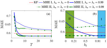
Figure 1: MAE performances of MHE for different values of $T$ and $b_{2}$. In (a), MHE I was implemented with $b_{2}=0.81$ and MHE II with $b_{2}=0.21$, and in (b) both MHEs had $T=15$. The shaded areas indicate the ranges of $b_{2}$ that meet the stability criteria of MHEs I and II as given in Lemmas 8-9.

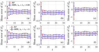
Figure 2: Mean error performances of KF and MHE I. MHE I was implemented with $\lambda_{w}$ and $\lambda_{v}$ both equal to 0.99 and 0 in (a)-(c) and in (d)-(f), respectively. In both cases, the two parameters were set as $T=15$ and $b_{2}=0.81$. The bars indicate the variations bounded by the standard deviations.

Alternatively, if the i-IOSS property is expressed by using a looser $\mathcal{K}\cdot\mathcal{L}$ bound with $\beta(s,t):=3.04s\cdot(t+1)^{\ln 0.9}$ (cf. Lemma 10 and the remark that follows), then by Lemma 8 a different valid cost function can be defined as:

$$V_{T}^{\prime}(\chi_{t-T},\thinspace\boldsymbol{\omega}_{t-T:t-1},\thinspace\boldsymbol{\nu}_{t-T:t})=\frac{|\chi_{t-T}-\hat{x}_{t-T}|^{2}}{\sigma_{0}^{2}(T+1)^{b_{2}}}\\ +V_{T,2}(\boldsymbol{\omega}_{t-T:t-1},\thinspace\boldsymbol{\nu}_{t-T:t}),$$ (23)

where $V_{T,2}(\boldsymbol{\omega}_{t-T:t-1},\thinspace\boldsymbol{\nu}_{t-T:t})$ is the same as in (22). To satisfy the stability conditions in Lemma 8, it is sufficient to choose $b_{2}=0.21$, which satisfies $0<b_{2}\leq-2\ln 0.9$. We call the resulting MHE as MHE II. Simulations were performed on the same random instances for different values of $T$ and $b_{2}$, and the results are again shown in Fig. 1. The state estimation results are slightly better than those obtained by MHE I for different values of $T$. Similar observations were yielded when the parameters $b_{2}$’s of the two MHEs took values in the ranges identified by Lemmas 8 and 9. Simulations also showed that both MHE I and MHE II remained stable even if $b_{2}$ took values beyond the identified ranges, which indicates the sufficiency but non-necessity of the derived stability conditions.

The solved optimizations are convex in both MHEs. The solution times averaged over the whole simulation period (i.e., 60 time units) and 100 random instances are summarized in Table I, for different sizes of moving horizons. The average solution times were less than 1.4 secs for both MHE I and MHE II if the parameters $\lambda_{w}$ and $\lambda_{v}$ were set to 0.99, and increased if $\lambda_{w}$ and $\lambda_{v}$ were set to 0 as the optimization became more challenging to solve. Moreover, in each case the solution time increased with the size of the moving horizon.

TABLE I: Average solution time (in secs) for the linear system.

Moving horizon size	5	10	15	20	25	30
Time for MHE I, with $\lambda_{w}=\lambda_{v}=0.99$	0.12	0.30	0.49	0.72	1.00	1.33
Time for MHE I, with $\lambda_{w}=\lambda_{v}=0$	0.60	1.48	2.24	2.93	3.49	3.92
Time for MHE II, with $\lambda_{w}=\lambda_{v}=0.99$	0.10	0.30	0.45	0.66	0.91	1.19
Time for MHE II, with $\lambda_{w}=\lambda_{v}=0$	0.60	1.46	2.11	2.58	3.16	3.79

Next, we compare the performances of MHE and KF when the measurements had outliers. In this case, the noise was a mixture of two truncated Gaussian noises: a nominal noise had a variance of $\sigma_{v}^{2}$ which occurred with a probability of $p$, and an intermittent large noise had a variance of $100\sigma_{v}^{2}$ which occurred with a probability of $(1-p)$ [31]. The system disturbances $w_{1,t}$, $w_{2,t}$ and $w_{3,t}$ were generated as the same Gaussian disturbance with a variance of $\sigma_{w}^{2}$. In the simulations, we set $p=0.9$, $\sigma_{v}=0.1$ and $\sigma_{w}=0.02$. The other simulation settings were the same as before. In this case, the cost function of the MHE was specified as

$$V_{T}(\chi_{t-T},\thinspace\boldsymbol{\omega}_{t-T:t-1},\thinspace\boldsymbol{\nu}_{t-T:t}):=\frac{|\chi_{t-T}-\hat{x}_{t-T}|^{2}b_{2}^{T}}{\sigma_{0}^{2}}\\ +\dfrac{\lambda_{w}}{\sigma_{w}^{2}T}\sum_{\tau=t-T}^{t-1}|\omega_{\tau}|^{2}+\dfrac{\lambda_{v}}{\sigma_{v}(T+1)}\sum_{\tau=t-T}^{t}|\nu_{\tau}|\\ +\dfrac{1-\lambda_{w}}{\sigma_{w}^{2}}\|\boldsymbol{\omega}_{t-T:t-1}\|^{2}+\dfrac{1-\lambda_{v}}{\sigma_{v}}\max_{\tau\in[t-T,\thinspace t]}|\nu_{\tau}|,$$

which imposes 1-norm instead of 2-norm penalties on the fitting errors $\{\nu_{\tau}\}_{t-T\leq\tau\leq t}$ in order to account for outliers in the measurements in a better manner [32, 33, 31]. The MHE also incorporates the knowledge of identical disturbances by including the equality constraints $\omega_{1,\tau}=\omega_{2,\tau}=\omega_{3,\tau}$ for all $\tau\in\mathbb{I}_{t-T:t-1}$. In contrast, the KF fully implemented 2-norm penalties, and the knowledge of identical disturbances was incorporated by specifying their covariance matrix as $\sigma_{w}^{2}\boldsymbol{1}_{3}$, where $\boldsymbol{1}_{3}$ is a $3\times 3$ matrix with all elements equal to 1.

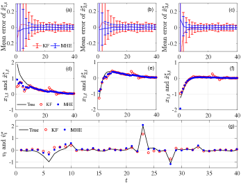
Figure 3: Performances of MHE and KF based on measurements with outliers. Subplots (a)-(c) present the mean estimation errors, and (d)-(g) show the estimates for a random instance.

As shown in Fig. 3(a)-(c), the state estimates obtained by MHE outperformed those obtained by KF during the whole simulation period, in terms of both mean and variance of the estimation errors. Fig. 3(d)-(f) show the true trajectories of the two states and their associated KF and MHE estimates in a random instance. The results confirm the superiority of MHE in this case. Indeed, this owes to the more accurate recovery of the measurement noise sequence by means of the 1-norm penalties applied on the measurement fitting errors, which is supported by the noise estimates shown in Fig. 3(g).

VI-B A nonlinear system

Consider a nonlinear continuous-time system described by

$$\left[\begin{array}[]{c}\dot{x}_{1,t}\\ \dot{x}_{2,t}\end{array}\right] =\left[\begin{array}[]{c}-2kx_{1,t}^{2}+w_{t}\\ kx_{1,t}^{2}\end{array}\right],$$ (24)

$$y_{t} =x_{1,t}+x_{2,t}+v_{t},\thinspace\thinspace\forall t\geq 0,$$

where $k=0.16$. When $w_{t}$ is constantly zero, the system describes an ideal gas-phase irreversible reaction in a well mixed, constant volume, isothermal batch reactor, where $x_{1,t}$ and $x_{2,t}$ represent the partial pressures and $y_{t}$ the reactor pressure measurement [34, 16]. In normal operations, the states and measurements are non-negative, i.e., $x_{1,t},\thinspace x_{2,t},\thinspace y_{t}\geq 0$ for all $t\geq 0$. We assume that $x_{2,0}\geq c_{0}$ for a certain positive constant $c_{0}$. This implies that $x_{2,t}\geq c_{0}>0$ for all $t\geq 0$ because $x_{2,t}$ increases with $t$.

First we prove that the system is i-IOSS, which was often assumed without a proof in the literature, e.g., [16]. Given two initial conditions $x_{0}^{(1)}:=[x_{1,0}^{(1)}\thinspace\thinspace x_{2,0}^{(1)}]^{\top}$ and $x_{0}^{(2)}:=[x_{1,0}^{(2)}\thinspace\thinspace x_{2,0}^{(2)}]^{\top}$, let the corresponding state trajectory be denoted as $x_{t}^{(1)}$ and $x_{t}^{(2)}$. Define $\delta x_{1,t}=x_{1,t}^{(1)}-x_{1,t}^{(2)}$ and $p_{t}=|\delta x_{1,t}|$. The dynamics of $p_{t}$ is then derived as

$$\dot{p}_{t} =\dfrac{\delta x_{1,t}}{|\delta x_{1,t}|}\delta\dot{x}_{1,t}=\dfrac{\delta x_{1,t}}{|\delta x_{1,t}|}\left(-2k(x_{1,t}^{(1)}+x_{1,t}^{(2)})\delta x_{1,t}+\delta w_{t}\right)$$

$$=-2k(x_{1,t}^{(1)}+x_{1,t}^{(2)})|\delta x_{1,t}|+\dfrac{\delta x_{1,t}}{|\delta x_{1,t}|}\delta w_{t}$$

$$\leq-2kc_{0}p_{t}+|\delta w_{t}|.$$

By the comparison lemma (Lemma 3.4 of [26]), it follows that

$$|\delta x_{1,t}| =p_{t}\leq p_{0}e^{-2kc_{0}t}+\int_{0}^{t}e^{-2kc_{0}(t-\tau)}|\delta w_{\tau}|d\tau$$

$$\leq|\delta x_{1,0}|e^{-2kc_{0}t}+\dfrac{1-e^{-2kc_{0}t}}{2kc_{0}}\left\|\delta\boldsymbol{w}_{0:t}\right\|$$

$$\leq|\delta x_{0}|e^{-2kc_{0}t}+\frac{\left\|\delta\boldsymbol{w}_{0:t}\right\|}{2kc_{0}}.$$

Therefore, the gap between the two full states is bounded as follows:

$$|x_{t}^{(1)}-x_{t}^{(2)}|\leq\left|\delta x_{1,t}\right|+\left|\delta x_{2,t}\right|\leq 2\left|\delta x_{1,t}\right|+\left|\delta(y_{t}-v_{t})\right|$$

$$\leq 2|\delta x_{0}|e^{-2kc_{0}t}+\dfrac{\left\|\delta\boldsymbol{w}_{0:t}\right\|}{kc_{0}}+\left\|\delta(\boldsymbol{y}_{0:t}-\boldsymbol{v}_{0:t})\right\|$$

$$=:\beta(|\delta x_{0}|,\thinspace t)+\alpha_{1}\left(\left\|\delta\boldsymbol{w}_{0:t}\right\|\right)+\alpha_{2}\left(\left\|\delta(\boldsymbol{y}_{0:t}-\boldsymbol{v}_{0:t})\right\|\right),$$

where $\beta\in\mathcal{KL}$ and $\alpha_{1},\alpha_{2}\in\mathcal{K}$. Thus, the system described in (24) is i-IOSS by Definition 2.

Let $w_{t}$ and $v_{t}$ be Gaussian white noises with variances equal to $0.001^{2}$ and $0.01^{2}$, respectively. And let the initial state $x_{0}$ follow a Gaussian distribution with a mean of $\bar{x}_{0}$ and a covariance of $\sigma_{0}^{2}I_{2}$, where $\bar{x}_{0}:=[0.1,\thinspace 4.5]$, $\sigma_{0}^{2}=9$ and $I_{2}$ is a $2\times 2$ identify matrix. In the simulations, we applied the Euler-Maruyama method [35] to obtain discrete counterparts of the stochastic differential equations in (24), and the discretization step size is given by $T_{s}$. According to Lemma 9, the MHE in discrete time is RGAS when the moving horizon size $T$ is large enough, if its cost function takes the form of (21)-(22) and is equipped with $b_{2}=e^{-4kc_{0}T_{s}}$. With $c_{0}=0.1$ and $T_{s}=0.1$ (smaller step sizes were found to yield similar results), Monte-Carlo simulations were performed for $T$ varying from 2 to 30 and the average state estimation results are shown in Fig. 4(a). As observed, MHE outperformed EKF once the moving horizon size $T$ is larger than 2 for $\lambda_{w}=\lambda_{v}=0.99$ and 4 for $\lambda_{w}=\lambda_{v}=0$. The observations were reflected in the results of a random instance as shown in Fig. 4(b)-(d), in which the prior estimate of the initial state was given by $\bar{x}_{0}$ and the MHE parameters were chosen as $\lambda_{w}=\lambda_{v}=0.99$ and $T=15$.

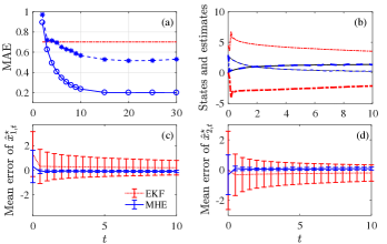
Figure 4: MAE and mean error performances of EKF and MHE. (a) MAE performances: the red dash-dot line is the results of EKF, and the blue dash curve with stars and the blue solid curve with circles correspond to the results of MHE with $\lambda_{w}$ and $\lambda_{v}$ both equal to 0, and 0.99. (b)-(d) The estimation results of a random instance: in (b) the black solid curves represent the true states, the blue dash and red dash-dot curves correspond to the MHE and the EKF estimates, and the thinner and the thicker curves refer to states $x_{1}$ and $x_{2}$, respectively; and mean errors of the two state estimates are shown in (c)-(d).

The computational times for solving the optimization problems in MHE with different sizes of moving horizons are summarized in Table II. Since the optimizations are nonlinear and non-convex, the computational times were much longer than those in the previous example in which the optimizations are convex. This reflects on the challenge that persists and needs to be tackled in MHE for nonlinear systems.

TABLE II: Average solution time (in secs) for the nonlinear system.

Moving horizon size	5	10	15	20	25	30
Time for MHE with $\lambda_{w}=\lambda_{v}=0.99$	0.32	0.70	1.21	1.78	2.62	3.59
Time for MHE with $\lambda_{w}=\lambda_{v}=0$	0.90	2.89	5.45	8.11	11.57	14.50

VII Discussion

This section provides a brief discussion on solving the optimization problem defined in (4) for MHE. If both the state and the measurement equations are linear, and if the bound sets are convex, then the optimization defined in (4) is convex when a convex cost function is used. In this case, the optimization problem can be solved efficiently to global optimality using state-of-the-art convex solvers [36], even if the MHE implements a large moving horizon size.

In practice, however, the state or the measurement equation is often nonlinear. This makes the optimization defined in (4) non-convex, and the computation for a global optimal solution becomes time-consuming. This tends to void the application of MHE in cases where computational time is a key concern. To tackle the challenge, researchers have proposed solving (4) for suboptimal solutions. For instance, in [12] the authors assume that the values of the cost function subjected to suboptimal solutions are within a fixed gap to the globally optimal costs. Yet it is unclear if there exist optimization solvers that can keep the assumption valid without violating the tight requirement on computational efficiency. In general, it remains an open challenge to ensure the RGAS of MHE when only suboptimal solutions are obtained for the series of optimization involved. Let the (global) optimal and the suboptimal solution of $(\chi_{t-T},\,\boldsymbol{\omega}_{t-T:t-1},\,\boldsymbol{\nu}_{t-T:t})$ be denoted as $(\hat{x}_{t-T},\,\hat{\boldsymbol{w}}_{t-T:t-1},\,\hat{\boldsymbol{v}}_{t-T:t})$ and $(\check{x}_{t-T},\,\check{\boldsymbol{w}}_{t-T:t-1},\,\check{\boldsymbol{v}}_{t-T:t})$, respectively. The following result may shed some light on the ways to tackle this challenge.

Theorem 3.

Given Assumption V.1 and any $\eta\in(0,\thinspace 1)$, the MHE which implements a suboptimal solution for the optimization in (4) is RGAS for all $T\geq T_{\eta,\bar{s}}$ if the following conditions are satisfied: a) the suboptimal solution yields a cost value which satisfies the following inequality,

$$V_{t}(\check{x}_{t-T},\,\check{\boldsymbol{w}}_{t-T:t-1},\,\check{\boldsymbol{v}}_{t-T:t})\\ \leq\gamma\left(V_{t}(\hat{x}_{t-T},\,\hat{\boldsymbol{w}}_{t-T:t-1},\,\hat{\boldsymbol{v}}_{t-T:t})\right)$$ (25)

with a certain $\gamma\in\mathcal{K}$; and b) the cost function of the associated FIE satisfies Assumption IV.1, a modified Assumption IV.2 and a modified inequality (16), in which the modifications are to replace the $\mathcal{KL}$ function $\rho_{x}$ and the $\mathcal{K}$ functions $\gamma_{w},\,\gamma_{v}$ used in Assumption IV.2 and inequality (16) with the $\mathcal{KL}$ function $\gamma\circ 3\rho_{x}$ and $\mathcal{K}$ functions $\gamma\circ 3\gamma_{w}$, $\gamma\circ 3\gamma_{v}$, respectively.

Proof:

By condition a) and Assumption IV.1, we have

$$\underline{\rho}_{x}(\left|\check{x}_{0}-\bar{x}_{0}\right|,t)+\underline{\gamma}_{w}(\left\|\check{\boldsymbol{w}}_{0:t-1}\right\|)+\underline{\gamma}_{v}(\left\|\check{\boldsymbol{v}}_{0:t}\right\|)$$

$$\leq V_{T}(\check{x}_{0}-\bar{x}_{0},\,\check{\boldsymbol{w}}_{0:t-1},\,\check{\boldsymbol{v}}_{0:t})$$

$$\leq\gamma\left(V_{T}(\hat{x}_{0}-\bar{x}_{0},\,\hat{\boldsymbol{w}}_{0:t-1},\,\hat{\boldsymbol{v}}_{0:t})\right)$$

$$\leq\gamma\left(V_{T}(x_{0}-\bar{x}_{0},\,\boldsymbol{w}_{0:t-1},\,\boldsymbol{v}_{0:t})\right)$$

$$\leq\gamma\left(\rho_{x}(\left|x_{0}-\bar{x}_{0}\right|,\,t)+\gamma_{w}(\left\|\boldsymbol{w}_{0:t-1}\right\|)+\gamma_{v}(\left\|\boldsymbol{v}_{0:t}\right\|)\right)$$

$$\leq\check{\rho}_{x}(\left|x_{0}-\bar{x}_{0}\right|,\,t)+\check{\gamma}_{w}(\left\|\boldsymbol{w}_{0:t-1}\right\|)+\check{\gamma}_{v}(\left\|\boldsymbol{v}_{0:t}\right\|)$$

where $\check{\rho}_{x}:=\gamma\circ 3\rho_{x}$, $\check{\gamma}_{w}:=\gamma\circ 3\gamma_{w}$ and $\check{\gamma}_{v}:=\gamma\circ 3\gamma_{v}$, which are $\mathcal{KL}$, $\mathcal{K}$ and $\mathcal{K}$ functions, respectively. The lower and the eventual upper bounds of $V_{T}(\check{x}_{0}-\bar{x}_{0},\,\check{\boldsymbol{w}}_{0:t-1},\,\check{\boldsymbol{v}}_{0:t})$ are in the same forms of the counterparts obtained for a global optimal solution (refer to part (a) of the proof of Theorem 1 in [15]). The only differences are that the left-hand side of the first inequality is expressed by the suboptimal instead of optimal solution variables, and that the right-hand side of the last inequality is described using the new functions $\check{\rho}_{x}$, $\check{\gamma}_{w}$ and $\check{\gamma}_{v}$, instead of $\rho_{x}$, $\gamma_{w}$ and $\gamma_{v}$. Consequently, under the modified Assumption IV.2, the proof of the associated FIE (which implements suboptimal solutions) being RGAS can be developed by following the same routine of part (a) of the proof of Theorem 1 in [15]. The remaining proof is to show that an additional condition, as a counterpart of (16), when the MHE implements suboptimal solutions, is also satisfied. This is done by applying the modified inequality (16) stated in condition b). The proof is then complete. ∎

Theorem 3 indicates that MHE can be RGAS even if it implements suboptimal solutions for the series of optimizations that are revealed over time. To that end, each suboptimal solution needs to satisfy certain conditions, say, inequality (25) which requires the yielded cost value to be upper bounded by a $\mathcal{K}$ function of the counterpart that results from an optimal solution. Since the condition does not restrict the form of the $\mathcal{K}$ function, it implies flexibility in obtaining the suboptimal solutions and hence also a direction for future research.

On the other hand, we may model the system dynamics and the measurements using discrete-time linear equations in which the disturbances and noises lump all unmodeled nonlinear dynamics (including unknown external disturbances and noises). This will enable MHE to solve only convex programs, but meanwhile may sacrifice the estimation accuracy for the increased uncertainties. Future research may be conducted to design appropriate convex MHEs that balance between the estimation accuracy and the computational complexity.

In addition, as remarked after the proof of Lemma 6, it is possible to change the size of the moving horizon of MHE online while keeping the MHE being RGAS. This will enable MHE with adaptive moving horizon which can be computationally more efficient on average as compared to the MHE that implements a moving horizon of a fixed size.

VIII Conclusion

This paper proved the robust global asymptotic stability (RGAS) of full information estimation (FIE) and its practical approximation, moving horizon estimation (MHE) under general settings. The results indicate that both FIE and MHE lead to bounded estimation errors under mild conditions for an incrementally input/output-to-state stable (i-IOSS) system subjected to bounded system and measurement disturbances. The stability conditions require that the cost function to be optimized has a property resembling the i-IOSS property of a system, but with a higher sensitivity to the uncertainty in the initial state. The stability of MHE additionally requires that the moving horizon is long enough to suppress temporal propagation of the estimator errors. Under the same conditions, the MHE was also shown to converge to the true state if the disturbances converge to zero in time.

When dealing with constrained nonlinear systems, MHE has to solve a non-convex program at each estimation point. Searching for a global optimal solution to the program requires considerable computational resources which are often unaffordable in applications. This problem has motivated considerable efforts to develop robustly stable MHE that relies on suboptimal but computationally more efficient solutions. We provided a brief discussion of this direction which may hopefully contribute to the future development of a systematic and practical solution for this equally important problem.

Appendix: A supporting lemma and its proof

Lemma 10.

Consider a system described by (2), where $f(x_{t},\thinspace w_{t})=Ax_{t}+g(x_{t})+w_{t}$ with $g$ being a nonlinear function, and $h$ is a linear or nonlinear measurement function. Suppose that $A$ is diagonalizable as $P^{-1}\Lambda P$ for a certain non-singular matrix $P$ and a diagonal matrix $\Lambda$. If the spectrum radius of $A$, denoted by $\rho(A)$, is less than one and the nonlinear functions satisfy $|g(x_{t}^{(1)})-g(x_{t}^{(2)})|\leq L|h(x_{t}^{(1)})-h(x_{t}^{(2)})|$ for all admissible $x_{t}^{(1)}$ and $x_{t}^{(2)}$ and a positive constant $L$, then the system is exp-i-IOSS as per (1), in which the $\mathcal{KL}$ function can be specified as $\beta(s,\thinspace t)=|P^{-1}||P|s\rho^{t}(A)\leq c_{1}s(t+1)^{-b_{1}}$ for all $s,\thinspace t\geq 0$, and the $\mathcal{K}$ functions as $\alpha_{1}(s)=\frac{|P^{-1}||P|}{1-\rho(A)}\cdot s$ and $\alpha_{2}(s)=\frac{L|P^{-1}||P|}{1-\rho(A)}\cdot s$ for all $s\geq 0$. Here the parameters $b_{1}$ and $c_{1}$ are positive constants satisfying $c_{1}\geq\max_{t\in\mathbb{I}_{\geq 0}}|P^{-1}||P|\rho^{t}(A)(t+1)^{b_{1}}$.

Proof:

Given two initial conditions $x_{0}^{(1)}$ and $x_{0}^{(2)}$ and corresponding disturbance sequences $\boldsymbol{w}_{0:t-1}^{(1)}$ and $\boldsymbol{w}_{0:t-1}^{(2)}$, let the system states at time $t$ be yielded as $x_{t}^{(1)}$ and $x_{t}^{(2)}$, respectively. By using the analytical expressions of the two states, we have

$$|x_{t}^{(1)}-x_{t}^{(2)}|$$

$$= \left|A^{t}(x_{0}^{(1)}-x_{0}^{(2)})+\sum_{l=0}^{t-1}A^{t-1-l}\left(g(x_{l}^{(1)})+w_{l}^{(1)}-g(x_{l}^{(2)})-w_{l}^{(2)}\right)\right|$$

$$\leq |A^{t}||x_{0}^{(1)}-x_{0}^{(2)}|+\left(\begin{array}[]{c}\|\boldsymbol{w}_{0:t-1}^{(1)}-\boldsymbol{w}_{0:t-1}^{(2)}\|\\ +\|g(\boldsymbol{x}_{0:t-1}^{(1)})-g(\boldsymbol{x}_{0:t-1}^{(2)})\|\end{array}\right)\sum_{k=0}^{t-1}|A^{k}|$$

$$\leq |P^{-1}||P|\left(\begin{array}[]{c}\rho^{t}(A)|x_{0}^{(1)}-x_{0}^{(2)}|\\ +\left(\begin{array}[]{c}\|\boldsymbol{w}_{0:t-1}^{(1)}-\boldsymbol{w}_{0:t-1}^{(2)}\|\\ +L\|h(\boldsymbol{x}_{0:t-1}^{(1)})-h(\boldsymbol{x}_{0:t-1}^{(2)})\|\end{array}\right)\sum_{k=0}^{t-1}\rho^{k}(A)\end{array}\right)$$

$$\leq |P^{-1}||P|\left(\begin{array}[]{c}\rho^{t}(A)|x_{0}^{(1)}-x_{0}^{(2)}|+\dfrac{1}{1-\rho(A)}\|\boldsymbol{w}_{0:t-1}^{(1)}-\boldsymbol{w}_{0:t-1}^{(2)}\|\\ +\dfrac{L}{1-\rho(A)}\|h(\boldsymbol{x}_{0:t}^{(1)})-h(\boldsymbol{x}_{0:t}^{(2)})\|\end{array}\right).$$

The last inequality implies that the system is i-IOSS and in particular exp-i-IOSS by Definition 2, in which the $\mathcal{KL}$ function $\beta$ and the $\mathcal{K}$ functions $\{\alpha_{1},\thinspace\alpha_{2}\}$ are specified by the lemma. Given $b_{1}\geq 0$, define $c_{1,\min}^{b_{1}}=\max_{t\in\mathbb{I}_{\geq 0}}|P^{-1}||P|\rho^{t}(A)(t+1)^{b_{1}}$. Since the maximum exists while $\rho(A)<1$, $c_{1,\min}^{b_{1}}$ is well defined. Therefore, there always exists $c_{1}\geq c_{1,\min}^{b_{1}}$ such that $|P^{-1}||P|\rho^{t}(A)\leq c_{1}(t+1)^{-b_{1}}$ for all $t\geq 0$. The conclusions of the lemma follows immediately. ∎

By the lemma, if a system is exp-i-IOSS with the $\mathcal{KL}$ bound function given as $\beta(s,\thinspace t)=c_{1}s^{a_{1}}b_{1}^{t}$ for certain positive constants $a_{1}$, $b_{1}$ and $c_{1}$ with $b_{1}<1$, then it is always feasible to specify a looser $\mathcal{KL}$ bound function as $\beta^{\prime}(s,\thinspace t)=c_{1}^{\prime}s^{a_{1}}(t+1)^{-b_{1}^{\prime}}$ for certain positive constants $b_{1}^{\prime}$ and $c_{1}^{\prime}$ satisfying $c_{1}^{\prime}\geq\max_{t\in\mathbb{I}_{\geq 0}}c_{1}b_{1}^{t}(t+1)^{b_{1}^{\prime}}$. For example, if $b_{1}^{\prime}$ is set to $1$, then $c_{1}^{\prime}$ can be specified as $\max c_{1}b_{1}^{t}(t+1)$ which exists for $t\in\mathbb{I}_{\geq 0}$ when $0\leq b_{1}<1$. For another example, if $b_{1}^{\prime}$ is set to $-\ln b_{1}$, then $c_{1}^{\prime}$ can be specified as equal to $c_{1}$ (which is equal to $\max_{t\in\mathbb{I}_{\geq 0}}c_{1}b_{1}^{t}(t+1)^{-\ln b_{1}}$).

Wuhua Hu received the BEng degree in Automation in 2005 and the MEng degree in Detecting Technique and Automation Device in 2007 from Tianjin University, China. He received the PhD degree in Communication Engineering from Nanyang Technological University (NTU), Singapore, in 2012. He is currently a Research Scientist with the Institute for Infocomm Research, Agency for Science, Technology and Research (A⋆STAR), Singapore. Before joining A⋆STAR, he worked as a Research Fellow first with the School of Mechanical and Aerospace Engineering and then the School of Electrical and Electronic Engineering, NTU, Singapore, from Aug 2011 to Mar 2016. His research interests lie in modeling, estimation, control and optimization of dynamical systems, with applications for smart and greener power and energy systems.

References

[1]
J. B. Rawlings, “Moving horizon estimation,” Encyclopedia of Systems
and Control, pp. 1–7, 2014.
[2]
A. Jazwinski, “Limited memory optimal filtering,” IEEE Trans. on Autom.
Control, vol. 13, no. 5, pp. 558–563, 1968.
[3]
K. R. Muske and J. B. Rawlings, “Nonlinear moving horizon state estimation,”
in Methods of Model Based Process Control, 1995, pp. 349–365.
[4]
F. Allgöwer, T. A. Badgwell, J. S. Qin, J. B. Rawlings, and S. J. Wright,
“Nonlinear predictive control and moving horizon estimation–an introductory
overview,” in Advances in Control, 1999, pp. 391–449.
[5]
J. Rawlings and L. Ji, “Optimization-based state estimation: Current status
and some new results,” Journal of Process Control, vol. 22, pp.
1439–1444, 2012.
[6]
K. R. Muske, J. B. Rawlings, and J. H. Lee, “Receding horizon recursive state
estimation,” in American Control Conference (ACC), San Francisco, CA,
USA, Jun 1993, pp. 900–904.
[7]
C. V. Rao, J. B. Rawlings, and J. H. Lee, “Constrained linear state
estimation–a moving horizon approach,” Automatica, vol. 37, no. 10,
pp. 1619–1628, 2001.
[8]
A. Alessandri, M. Baglietto, and G. Battistelli, “Receding-horizon estimation
for discrete-time linear systems,” IEEE Trans. on Autom. Control,
vol. 48, no. 3, pp. 473–478, 2003.
[9]
H. Michalska and D. Q. Mayne, “Moving horizon observers and observer-based
control,” IEEE Trans. on Autom. Control, vol. 40, no. 6, pp.
995–1006, 1995.
[10]
A. Alessandri, M. Baglietto, T. Parisini, and R. Zoppoli, “A neural state
estimator with bounded errors for nonlinear systems,” IEEE Trans. on
Autom. Control, vol. 44, no. 11, pp. 2028–2042, 1999.
[11]
C. Rao, J. Rawlings, and D. Mayne, “Constrained state estimation for nonlinear
discrete-time systems: Stability and moving horizon approximations,”
IEEE Trans. on Autom. Control, vol. 48, no. 2, pp. 246–258, 2003.
[12]
A. Alessandri, M. Baglietto, and G. Battistelli, “Moving-horizon state
estimation for nonlinear discrete-time systems: New stability results and
approximation schemes,” Automatica, vol. 44, no. 7, pp. 1753–1765,
2008.
[13]
A. Alessandri, M. Baglietto, G. Battistelli, and V. Zavala, “Advances in
moving horizon estimation for nonlinear systems,” in The 49th IEEE
Conference on Decision and Control (CDC), Atlanta, Georgia, USA, Dec. 2010,
pp. 5681–5688.
[14]
J. Liu, “Moving horizon state estimation for nonlinear systems with bounded
uncertainties,” Chem. Eng. Sci., vol. 93, pp. 376–386, 2013.
[15]
W. Hu, L. Xie, and K. You, “Optimization-based state estimation under bounded
disturbances,” in The 54th IEEE Conference on Decision and Control
(CDC), Osaka, Japan, Dec 2015.
[16]
L. Ji, J. B. Rawlings, W. Hu, A. Wynn, and M. Diehl, “Robust stability of
moving horizon estimation under bounded disturbances,” IEEE Trans. on
Autom. Control, vol. 61, no. 11, pp. 3509 – 3514, 2016.
[17]
M. A. Müller, “Nonlinear moving horizon estimation in the presence of
bounded disturbances,” Automatica, vol. 79, pp. 306–314, 2017.
[18]
E. Sontag and Y. Wang, “Output-to-state stability and detectability of
nonlinear systems,” Systems & Control Letters, vol. 29, no. 5, pp.
279–290, 1997.
[19]
J. B. Rawlings and D. Q. Mayne, Model Predictive Control: Theory and
Design. Madison, WI: Nob Hill Pub.,
2009.
[20]
V. M. Zavala, C. D. Laird, and L. T. Biegler, “A fast moving horizon
estimation algorithm based on nonlinear programming sensitivity,”
Journal of Process Control, vol. 18, no. 9, pp. 876–884, 2008.
[21]
P. Kühl, M. Diehl, T. Kraus, J. P. Schlöder, and H. G. Bock, “A
real-time algorithm for moving horizon state and parameter estimation,”
Computers & Chemical Engineering, vol. 35, no. 1, pp. 71–83, 2011.
[22]
R. López-Negrete and L. T. Biegler, “A moving horizon estimator for
processes with multi-rate measurements: A nonlinear programming sensitivity
approach,” Journal of Process Control, vol. 22, no. 4, pp. 677–688,
2012.
[23]
A. Wynn, M. Vukov, and M. Diehl, “Convergence guarantees for moving horizon
estimation based on the real-time iteration scheme,” IEEE Trans. on
Autom. Control, vol. 59, no. 8, pp. 2215–2221, 2014.
[24]
A. Alessandri and M. Gaggero, “Moving-horizon estimation for discrete-time
linear and nonlinear systems using the gradient and newton methods,” in
IEEE 55th Conference on Decision and Control (CDC), Melbourne,
Australia, Dec. 2016, pp. 2906–2911.
[25]
L. Ljung, “Asymptotic behavior of the extended kalman filter as a parameter
estimator for linear systems,” IEEE Trans. on Autom. Control,
vol. 24, no. 1, pp. 36–50, 1979.
[26]
H. K. Khalil, Nonlinear Systems, 3rd ed. Upper Saddle River, NJ: Prentice Hall, 2002.
[27]
L. Grüne, “Input-to-state stability of exponentially stabilized semilinear
control systems with inhomogeneous perturbations,” Systems & Control
Letters, vol. 38, no. 1, pp. 27–35, 1999.
[28]
B. Liu, D. J. Hill, and Y. Sun, “Exponential input-to-state stability for
hybrid dynamical networks via impulsive interconnection,” in The 49th
IEEE Conference on Decision and Control (CDC), Atlanta, Georgia, USA, Dec
2010, pp. 673–678.
[29]
E. D. Sontag, “Comments on integral variants of ISS,” Systems &
Control Letters, vol. 34, no. 1, pp. 93–100, 1998.
[30]
M. D. Glas, “Exponential stability revisited,” International Journal of
Control, vol. 46, no. 5, pp. 1505–1510, 1987.
[31]
A. Aravkin, J. V. Burke, L. Ljung, A. Lozano, and G. Pillonetto, “Generalized
kalman smoothing: Modeling and algorithms,” arXiv preprint
arXiv:1609.06369, 2016.
[32]
Q. Ke and T. Kanade, “Robust L1 norm factorization in the presence of
outliers and missing data by alternative convex programming,” in IEEE
Computer Society Conference on Computer Vision and Pattern Recognition,
Seattle, WA, USA, Jun 2005.
[33]
J. D. Hedengren and A. N. Eaton, “Overview of estimation methods for
industrial dynamic systems,” Optimization and Engineering, pp. 1–24,
2015.
[34]
E. Haseltine and J. Rawlings, “Critical evaluation of extended kalman
filtering and moving-horizon estimation,” Industrial & Engineering
Chemistry Research, vol. 44, no. 8, pp. 2451–2460, 2005.
[35]
D. J. Higham, “An algorithmic introduction to numerical simulation of
stochastic differential equations,” SIAM Review, vol. 43, no. 3, pp.
525–546, 2001.
[36]
S. Boyd and L. Vandenberghe, Convex Optimization. Cambridge, UK: Cambridge University Press, 2004.